Revisiting Graph Neural Networks:
All We Have is Low-Pass Filters

Abstract

Graph neural networks have become one of the most important techniques to solve machine learning problems on graph-structured data. Recent work on vertex classification proposed deep and distributed learning models to achieve high performance and scalability. However, we find that the feature vectors of benchmark datasets are already quite informative for the classification task, and the graph structure only provides a means to denoise the data. In this paper, we develop a theoretical framework based on graph signal processing for analyzing graph neural networks. Our results indicate that graph neural networks only perform low-pass filtering on feature vectors and do not have the non-linear manifold learning property. We further investigate their resilience to feature noise and propose some insights on GCN-based graph neural network design.

1 Introduction

Graph neural networks (GNN) belong to a class of neural networks which can learn from graph-structured data. Recently, graph neural networks for vertex classification and graph isomorphism test have achieved excellent results on several benchmark datasets and continuously set new state-of-the-art performance Abu-El-Haija et al. (2019); Kipf and Welling (2017); Veličković et al. (2017); Xu et al. (2019). Started with the early success of ChebNet Defferrard et al. (2016) and GCN Kipf and Welling (2017) at vertex classification, many variants of GNN have been proposed to solve problems in social networks Hamilton et al. (2017); Zhang et al. (2018a), biology Veličković et al. (2017, 2019), chemistry Fout et al. (2017); Gilmer et al. (2017), natural language processing Bastings et al. (2017); Zhang et al. (2018b), computer vision Santoro et al. (2017), and weakly-supervised learning Garcia and Bruna (2017).

In semi-supervised vertex classification, we observe that the parameters of a graph convolutional layer in a Graph Convolutional Network (GCN) Kipf and Welling (2017) only contribute to overfitting. Similar observations have been reported in both simple architectures such as SGC Wu et al. (2019) and more complex ones such as DGI Veličković et al. (2019). Based on this phenomenon, Wu et al. (2019) proposed to view graph neural networks simply as feature propagation and propose an extremely efficient model with state-of-the-art performance on many benchmark datasets. Kawamoto et al. (2018) made a related theoretical remark on untrained GCN-like GNNs under graph partitioning settings. From these previous studies, a question naturally arises: Why and when do graph neural networks work well for vertex classification? In other words, is there a condition on the vertex feature vectors for graph neural network models to work well even without training? Consequently, can we find realistic counterexamples in which baseline graph neural networks (e.g. SGC or GCN) fail to perform?

In this study, we provide an answer to the aforementioned questions from the graph signal processing perspective Ortega et al. (2018). Formally, we consider a semi-supervised learning problem on a graph. Given a graph $𝒢=(𝒱,ℰ)$, each vertex $i\in 𝒱$ has a feature $𝐱(i)\in 𝒳$ and label $y(i)\in 𝒴$, where $𝒳$ is a $d$-dimensional Euclidean space ${ℝ}^d$ and $𝒴=ℝ$ for regression and $𝒴=\{1,\mathrm{\dots },c\}$ for classification. The task is to learn a hypothesis to predict the label $y(i)$ from the feature $𝐱(i)$. We then characterize the graph neural networks solution to this problem and provide insights to the mechanism underlying the most commonly used baseline model GCN Kipf and Welling (2017), and its simplified variant SGC Wu et al. (2019).

Figure 1: Accuracy by frequency components

Figure 2: A simple realization of gfNN

Graph signal processing (GSP) regards data on the vertices as signals and applies signal processing techniques to understand the signal characteristics. By combining signals (feature vectors) and graph structure (adjacency matrix or its transformations), GSP has inspired the development of learning algorithms on graph-structured data Shuman et al. (2012). In a standard signal processing problem, it is common to assume the observations contain some noise and the underlying “true signal” has low-frequency Rabiner and Gold (1975). Here, we pose a similar assumption for our problem.

Assumption 1.

Input features consist of low-frequency true features and noise. The true features have sufficient information for the machine learning task.

Our first contribution is to verify Assumption 1 on commonly used datasets (Section 3). Figure 1 shows the performance of 2-layers perceptrons (MLPs) trained on features with different numbers of frequency components. In all benchmark datasets, we see that only a small number of frequency components contribute to learning. Adding more frequency components to the feature vectors only decreases the performance. In turn, the classification accuracy becomes even worse when we add Gaussian noise $𝒩(0,{\sigma }^2)$ to the features.

Many recent GNNs were built upon results from graph signal processing. The most common practice is to multiply the (augmented) normalized adjacency matrix $I-\widetilde{ℒ}$ with the feature matrix $𝒳$. The product $(I-\widetilde{ℒ})𝒳$ is understood as features averaging and propagation Hamilton et al. (2017); Kipf and Welling (2017); Wu et al. (2019). In graph signal processing literature, such operation filters signals on the graph without explicitly performing eigendecomposition on the normalized Laplacian matrix, which requires $O(n^3)$ time Vaseghi (2008). Here, we refer to this augmented normalized adjacency matrix and its variants as graph filters and propagation matrices interchangeably.

Our second contribution shows that multiplying graph signals with propagation matrices corresponds to low-pass filtering (Section 4, esp., Theorem 3). Furthermore, we also show that the matrix product between the observed signal and the low-pass filters is the analytical solution to the true signal optimization problem. In contrast to the recent design principle of graph neural networks Abu-El-Haija et al. (2019); Kipf and Welling (2017); Xu et al. (2019), our results suggest that the graph convolution layer is simply low-pass filtering. Therefore, learning the parameters of a graph convolution layer is unnecessary. Wu et al. (2019, Theorem 1) also addressed a similar claim by analyzing the spectrum-truncating effect of the augmented normalized adjacency matrix. We extend this result to show that all eigenvalues monotonically shrink, which further explains the implications of the spectrum-truncating effect.

Based on our theoretical understanding, we propose a new baseline framework named gfNN (graph filter neural network) to empirically analyze the vertex classification problem. gfNN consists of two steps: 1. Filter features by multiplication with graph filter matrices; 2. Learn the vertex labels by a machine learning model. We demonstrate the effectiveness of our framework using a simple realization model in Figure 2.

Our third contribution is the following Theorem:

Theorem 2 (Informal, see Theorem 7, 8).

Under Assumption 1, the outcomes of SGC, GCN, and gfNN are similar to those of the corresponding NNs using true features.

Theorem 7 implies that, under Assumption 1, both gfNN and GCN Kipf and Welling (2017) have similar high performance. Since gfNN does not require multiplications of the adjacency matrix during the learning phase, it is much faster than GCN. In addition, gfNN is also more noise tolerant.

Finally, we compare our gfNN to the SGC model Wu et al. (2019). While SGC is also computationally fast and accurate on benchmark datasets, our analysis implies it would fail when the feature input is nonlinearly-separable because the graph convolution part does not contribute to non-linear manifold learning. We created an artificial dataset to empirically demonstrate this claim.

2 Graph Signal Processing

In this section, we introduce the basic concepts of graph signal processing. We adopt a recent formulation Girault et al. (2018) of graph Fourier transform on irregular graphs.

Let $𝒢=(𝒱,ℰ)$ be a simple undirected graph, where $𝒱=\{1,\mathrm{\dots },n\}$ be the set of $n\in \mathbb{Z}$ vertices and $ℰ$ be the set of edges. Let $A=(a_{ij})\in {ℝ}^{n\times n}$ be the adjacency matrix of $G$, $D=\mathrm{diag}(d(1),\mathrm{\dots },d(n))\in {ℝ}^{n\times n}$ be the degree matrix of $G$, where $d(i)={\sum }_{j\in 𝒱}a(i,j)$ is the degree of vertex $i\in 𝒱$. $L=D-A\in {ℝ}^{n\times n}$ be the combinatorial Laplacian of $G$, $ℒ=I-D^{-1/2}A{D}^{-1/2}$ be the normalized Laplacian of $G$, where $I\in {ℝ}^{n\times n}$ is the identity matrix, and $L_{\text{rw}}=I-D^{-1}A$ be the random walk Laplacian of $G$. Also, for $\gamma \in ℝ$ with $\gamma >0$, let $\tilde{A}=A+\gamma I$ be the augmented adjacency matrix, which is obtained by adding $\gamma$ self loops to $G$, $\tilde{D}=D+\gamma I$ be the corresponding augmented degree matrix, and $\tilde{L}=\tilde{D}-\tilde{A}=L$, $\widetilde{ℒ}=I-{\tilde{D}}^{-1/2}\tilde{A}{\tilde{D}}^{-1/2}$, ${\tilde{L}}_{\text{rw}}=I-{\tilde{D}}^{-1}\tilde{A}$ be the corresponding augmented combinatorial, normalized, and random walk Laplacian matrices.

A vector $x\in {ℝ}^n$ defined on the vertices of the graph is called a graph signal. To introduce a graph Fourier transform, we need to define two operations, variation and inner product, on the space of graph signals. Here, we define the variation $\mathrm{\Delta }:{ℝ}^n\to ℝ$ and the $\tilde{D}$-inner product by

$\mathrm{\Delta }(x):={\displaystyle \sum _{(i,j)\in ℰ}}{(x(i)-x(j))}^2=x^{\top }Lx;{(x,y)}_{\tilde{D}}:={\displaystyle \sum _{i\in 𝒱}}(d(i)+\gamma )x(i)y(i)=x^{\top }\tilde{D}y.$ (1)

We denote by ${\Vert x\Vert }_{\tilde{D}}:=\sqrt{{(x,x)}_{\tilde{D}}}$ the norm induced by $\tilde{D}$. Intuitively, the variation $\mathrm{\Delta }$ and the inner product ${(\cdot ,\cdot )}_{\tilde{D}}$ specify how to measure the smoothness and importance of the signal, respectively. In particular, our inner product puts more importance on high-degree vertices, where larger $\gamma$ closes the importance more uniformly. We then consider the generalized eigenvalue problem (variational form): Find $u_1,\mathrm{\dots },u_n\in {ℝ}^n$ such that for each $i\in \{1,\mathrm{\dots },n\}$, $u_i$ is a solution to the following optimization problem:

$\text{minimize}\mathrm{\Delta }(u)\text{subject to}{(u,u)}_{\tilde{D}}=1,{(u,u_j)}_{\tilde{D}}=0,j\in \{1,\mathrm{\dots },n\}.$ (2)

The solution $u_i$ is called an $i$-th generalized eigenvector and the corresponding objective value ${\lambda }_i:=\mathrm{\Delta }(u_i)$ is called the $i$-th generalized eigenvalue. The generalized eigenvalues and eigenvectors are also the solutions to the following generalized eigenvalue problem (equation form):

$Lu=\lambda \tilde{D}u.$ (3)

Thus, if $(\lambda ,u)$ is a generalized eigenpair then $(\lambda ,{\tilde{D}}^{1/2}u)$ is an eigenpair of $\widetilde{ℒ}$. A generalized eigenvector with a smaller generalized eigenvalue is smoother in terms of the variation $\mathrm{\Delta }$. Hence, the generalized eigenvalues are referred to as the frequency of the graph.

The graph Fourier transform is a basis expansion by the generalized eigenvectors. Let $U=[u_1,\mathrm{\dots },u_n]$ be the matrix whose columns are the generalized eigenvectors. Then, the graph Fourier transform $ℱ\mathrm{:}{ℝ}^n\mathrm{\to }{ℝ}^n$ is defined by $ℱx=\widehat{x}:=U^{\top }\tilde{D}x$, and the inverse graph Fourier transform ${ℱ}^{\mathrm{-}\mathrm{1}}$ is defined by ${ℱ}^{-1}\widehat{x}=U\widehat{x}$. Note that these are actually the inverse transforms since $ℱ{ℱ}^{-1}=U^{\top }\tilde{D}U=I$.

The Parseval identity relates the norms of the data and its Fourier transform:

${\Vert x\Vert }_{\tilde{D}}={\Vert \widehat{x}\Vert }_2.$ (4)

Let $h:ℝ\to ℝ$ be an analytic function. The graph filter specified by $h$ is a mapping $x\mapsto y$ defined by the relation in the frequency domain: $\widehat{y}(\lambda )=h(\lambda )\widehat{x}(\lambda )$. In the spatial domain, the above equation is equivalent to $y=h({\tilde{L}}_{\text{rw}})x$. where $h({\tilde{L}}_{\text{rw}})$ is defined via the Taylor expansion of $h$; see Higham (2008) for the detail of matrix functions.

In a machine learning problem on a graph, each vertex $i\in 𝒱$ has a $d$-dimensional feature $𝐱(i)\in {ℝ}^d$. We regard the features as $d$ graph signals and define the graph Fourier transform of the features by the graph Fourier transform of each signal. Let $X={[𝐱(1);\mathrm{\dots },𝐱(n)]}^{\top }$ be the feature matrix. Then, the graph Fourier transform is represented by $ℱX=\widehat{X}=:U^{\top }\tilde{D}X$ and the inverse transform is ${ℱ}^{-1}\widehat{X}=U\widehat{X}$. We denote $\widehat{X}={[\widehat{𝐱}({\lambda }_1);\mathrm{\dots };\widehat{𝐱}({\lambda }_n)]}^{\top }$ as the frequency components of $X$.

3 Empirical Evidence of Assumption 1

The results of this paper deeply depend on Assumption 1. Thus, we first verify this assumption in real-world datasets: Cora, Citeseer, and Pubmed Sen et al. (2008). These are citation networks, in which vertices are scientific papers and edges are citations. We consider the following experimental setting: 1. Compute the graph Fourier basis $U$ from $\widetilde{ℒ}$; 2. Add Gaussian noise to the input features: $𝒳\leftarrow 𝒳+𝒩(0,{\sigma }^2)$ for $\sigma =\{0,0.01,0.05\}$; 3. Compute the first $k$-frequency component: ${\widehat{𝒳}}_k=U{[:k]}^{\top }{\tilde{D}}^{1/2}𝒳$; 4. Reconstruct the features: ${\widetilde{𝒳}}_k={\tilde{D}}^{-1/2}U[:k]{\widehat{𝒳}}_k$; 5. Train and report test accuracy of a 2-layers perceptron on the reconstructed features ${\widetilde{𝒳}}_k$.

Figure 3: Average performance of 2-layers MLPs on frequency-limited feature vectors (epochs=20). The annotated “(best)” horizontal lines show the performance of the best performance using gfNN and a 2-layers MLP trained on the original features.

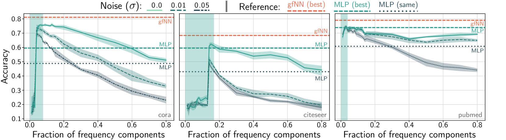
In Figure 3, we incrementally add normalized Laplacian frequency components to reconstruct feature vectors and train a 2-layers MLPs. We see that all three datasets exhibit a low-frequency nature. The classification accuracy of a 2-layers MLP tends to peak within the top 20% of the spectrum (green boxes). By adding artificial Gaussian noise, we observe that the performance at low-frequency regions is relatively robust, which implies a strong denoising effect.

Interestingly, the performance gap between graph neural network and a simple MLP is much larger when high-frequency components do not contain useful information for classification. In the Cora dataset, high-frequency components only decrease classification accuracy. Therefore, our gfNN outperformed a simple MLP. Citeseer and Pubmed have a similar low-frequency nature. However, the performance gaps here are not as large. Since the noise-added performance lines for Citeseer and Pubmed generally behave like the original Cora performance line, we expect the original Citeseer and Pubmed contain much less noise compared with Cora. Therefore, we could expect the graph filter degree would have little effect in Citeseer and Pubmed cases.

4 Multiplying Adjacency Matrix is Low Pass Filtering

Computing the low-frequency components is expensive since it requires $O({|𝒱|}^3)$ time to compute the eigenvalue decomposition of the Laplacian matrix. Thus, a reasonable alternative is to use a low-pass filter. Many papers on graph neural networks iteratively multiply the (augmented) adjacency matrix ${\tilde{A}}_{\text{rw}}$ (or $\tilde{A}$) to propagate information. In this section, we see that this operation corresponds to a low-pass filter.

Multiplying the normalized adjacency matrix corresponds to applying graph filter $h(\lambda )=1-\lambda$. Since the eigenvalues of the normalized Laplacian lie on the interval $[0,2]$, this operation resembles a band-stop filter that removes intermediate frequency components. However, since the maximum eigenvalue of the normalized Laplacian is $2$ if and only if the graph contains a non-trivial bipartite graph as a connected component (Chung, 1997, Lemma 1.7). Therefore, for other graphs, multiplying the normalized (non-augmented) adjacency matrix acts as a low-pass filter (i.e., high-frequency components must decrease).

We can increase the low-pass filtering effect by adding self-loops (i.e., considering the augmented adjacency matrix) since it shrinks the eigenvalues toward zero as follows.

Theorem 3.

Let ${\lambda }_i\mathit{}\mathrm{(}\gamma \mathrm{)}$ be the $i$-th smallest generalized eigenvalue of $\mathrm{(}\stackrel{\mathrm{~}}{D}\mathrm{,}L\mathrm{)}\mathrm{=}\mathrm{(}D\mathrm{+}\gamma \mathit{}I\mathrm{)}$. Then, ${\lambda }_i\mathit{}\mathrm{(}\gamma \mathrm{)}$ is a non-negative number, and monotonically non-increasing in $\gamma \mathrm{\ge }\mathrm{0}$. Moreover, ${\lambda }_i\mathit{}\mathrm{(}\gamma \mathrm{)}$ is strictly monotonically decreasing if ${\lambda }_i\mathit{}\mathrm{(}\mathrm{0}\mathrm{)}\mathrm{\ne }\mathrm{0}$.

Note that $\gamma$ cannot be too large. Otherwise, all the eigenvalues would be concentrated around zero, i.e., all the data would be regarded as “low-frequency”; hence, we cannot extract useful information from the low-frequency components.

The graph filter $h(\lambda )=1-\lambda$ can also be derived from a first-order approximation of a Laplacian regularized least squares Belkin and Niyogi (2004). Let us consider the problem of estimating a low-frequency true feature ${\{\overline{𝐱}(i)\}}_{i\in 𝒱}$ from the observation ${\{𝐱(i)\}}_{i\in 𝒱}$. Then, a natural optimization problem is given by

$\underset{\overline{x}}{\min }{\displaystyle \sum _{i\in 𝒱}}{\Vert \overline{𝐱}(i)-𝐱(i)\Vert }_{\tilde{D}}^2+\mathrm{\Delta }(\overline{X})$ (5)

where $\mathrm{\Delta }(\overline{X})={\sum }_{p=1}^d\mathrm{\Delta }(\overline{𝐱}{(i)}_p)$. Note that, since $\mathrm{\Delta }(\overline{X})={\sum }_{\lambda \in \mathrm{\Lambda }}\lambda {\Vert \widehat{\overline{𝐱}}(\lambda )\Vert }_2^2$, it is a maximum a posteriori estimation with the prior distribution of $\widehat{\overline{𝐱}}(\lambda )\sim N(0,I/\lambda )$. The optimal solution to this problem is given by $\overline{X}={(I+{\tilde{L}}_{\text{rw}})}^{-1}X$. The corresponding filter is $h^{\prime }(\lambda )={(1+\lambda )}^{-1}$, and hence $h(\lambda )=1-\lambda$ is its first-order Taylor approximation.

5 Bias-Variance Trade-off for Low Pass Filters

In the rest of this paper, we establish theoretical results under Assumption 1. To be concrete, we pose a more precise assumption as follows.

Assumption 4 (Precise Version of the First Part of Assumption 1).

Observed features ${\mathrm{\{}𝐱\mathit{}\mathrm{(}i\mathrm{)}\mathrm{\}}}_{i\mathrm{\in }𝒱}$ consists of true features ${\mathrm{\{}\overline{𝐱}\mathit{}\mathrm{(}i\mathrm{)}\mathrm{\}}}_{i\mathrm{\in }𝒱}$ and noise ${\mathrm{\{}𝐳\mathit{}\mathrm{(}i\mathrm{)}\mathrm{\}}}_{i\mathrm{\in }𝒱}$. The true features $\overline{X}$ have frequency at most $\mathrm{0}\mathrm{\le }ϵ\mathrm{\ll }\mathrm{1}$ and the noise follows a white Gaussian noise, i.e., each entry of the graph Fourier transform of $Z$ independently identically follows a normal distribution $N\mathit{}\mathrm{(}\mathrm{0}\mathrm{,}{\sigma }^{\mathrm{2}}\mathrm{)}$.

Using this assumption, we can evaluate the effect of the low-pass filter as follows.

Lemma 5.

Suppose Assumption 4. For any , with probability at least $\mathrm{1}\mathrm{-}\delta$, we have

${\Vert \overline{X}-{\tilde{A}}_{\text{𝑟𝑤}}^{k}X\Vert }_D\le \sqrt{kϵ}{\Vert \overline{X}\Vert }_D+O\left(\sqrt{\log (1/\delta )R(2k)}\right)𝔼[{\Vert Z\Vert }_D],$ (6)

where $R\mathit{}\mathrm{(}\mathrm{2}\mathit{}k\mathrm{)}$ is a probability that a random walk with a random initial vertex returns to the initial vertex after $\mathrm{2}\mathit{}k$ steps.

The first and second terms of the right-hand side of (6) are the bias term incurred by applying the filter and the variance term incurred from the filtered noise, respectively. Under the assumption, the bias increases a little, say, $O(\sqrt{ϵ})$. The variance term decreases in $O(1/{\mathrm{deg}}^{k/2})$ where $\mathrm{deg}$ is a typical degree of the graph since $R(2k)$ typically behaves like $O(1/{\mathrm{deg}}^k)$ for small $k$. Therefore, we can obtain a more accurate estimation of the true data from the noisy observation by multiplying the adjacency matrix if the maximum frequency of $\overline{X}$ is much smaller than the noise-to-signal ratio ${\Vert Z\Vert }_D/{\Vert \overline{X}\Vert }_D$.

This theorem also suggest a choice of $k$. By minimizing the right-hand side by $k$, we obtain:

Corollary 6.

Suppose that $𝔼\mathit{}\mathrm{[}{\mathrm{\Vert }Z\mathrm{\Vert }}_D\mathrm{]}\mathrm{\le }\rho \mathit{}{\mathrm{\Vert }\overline{X}\mathrm{\Vert }}_D$ for some $\rho \mathrm{=}O\mathit{}\mathrm{(}\mathrm{1}\mathrm{)}$. Let $k^{\mathrm{*}}$ be defined by $k^{\mathrm{*}}\mathrm{=}O\mathit{}\mathrm{(}\log \mathit{}\mathrm{(}\log \mathit{}\mathrm{(}\mathrm{1}\mathrm{/}\delta \mathrm{)}\mathit{}\rho \mathrm{/}ϵ\mathrm{)}\mathrm{)}$, and suppose that there exist constants $C_d$ and $\overline{d}\mathrm{>}\mathrm{1}$ such that $R\mathit{}\mathrm{(}\mathrm{2}\mathit{}k\mathrm{)}\mathrm{\le }{C}_d\mathrm{/}{\overline{d}}^k$ for $k\mathrm{\le }{k}^{\mathrm{*}}$. Then, by choosing $k\mathrm{=}{k}^{\mathrm{*}}$, the right-hand side of (6) is $\stackrel{\mathrm{~}}{O}\mathit{}\mathrm{(}\sqrt{ϵ}\mathrm{)}$. ∎

This concludes that we can obtain an estimation of the true features with accuracy $\tilde{O}(\sqrt{ϵ})$ by multiplying ${\tilde{A}}_{\text{rw}}$ several times.

6 Graph Filter Neural Network

In the previous section, we see that low-pass filtered features ${\tilde{A}}_{\text{rw}}^{k}X$ are accurate estimations of the true features with high probability. In this section, we analyze the performance of this operation.

Let the multi-layer (two-layer) perceptron be

$h_{\text{MLP}}(X|W_1,W_2)$ $={\sigma }_2({\sigma }_1(X{W}_1)W_2),$ (7)

where ${\sigma }_1$ is the entry-wise ReLU function, and ${\sigma }_2$ is the softmax function. Note that both ${\sigma }_1$ and ${\sigma }_2$ are contraction maps, i.e., ${\Vert {\sigma }_i(X)-\sigma (Y)\Vert }_D\le {\Vert X-Y\Vert }_D$.

Under the second part of Assumption 1, our goal is to obtain a result similar to $h(\overline{X}|W_1,W_2)$. The simplest approach is to train a multi-layer perceptron $h_{\text{MLP}}(X|W_1,W_2)$ with the observed feature. The performance of this approach is evaluated by

$\parallel h_{\text{MLP}}(\overline{X}|W_1,W_2)-h_{\text{MLP}}(X|W_1,W_2){\parallel }_{\tilde{D}}\le \parallel Z{\parallel }_D\rho (W_1)\rho (W_2),$ (8)

where $\rho (W)$ is the maximum singular value of $W$.

Now, we consider applying graph a filter ${\tilde{A}}_{\text{rw}}^k$ to the features, then learning with a multi-layer perceptron, i.e., $h_{\text{MLP}}(h({\tilde{L}}_{\text{rw}})X|W_1,W_2)$. Using Lemma 5, we obtain the following result.

Theorem 7.

Suppose Assumption 4 and conditions in Corollary 6. By choosing $k$ as Corollary 6, with probability at least $\mathrm{1}\mathrm{-}\delta$ for ,

$\parallel h_{\text{𝑀𝐿𝑃}}(\overline{X}|W_1,W_2)-h_{\text{𝑀𝐿𝑃}}({\tilde{A}}_{\text{𝑟𝑤}}^{2}X|W_1,W_2){\parallel }_D=\tilde{O}(\sqrt{ϵ})𝔼[\parallel Z{\parallel }_D]\rho (W_1)\rho (W_2).$ (9)

∎

This means that if the maximum frequency of the true data is small, we obtain a solution similar to the optimal one.

Comparison with GCN

Under the same assumption, we can analyze the performance of a two-layers GCN. The GCN is given by

$h_{\text{GCN}}(X|W_1,W_2)$ $={\sigma }_2({\tilde{A}}_{\text{rw}}{\sigma }_1({\tilde{A}}_{\text{rw}}X{W}_1)W_2).$ (10)

Theorem 8.

Under the same assumption to Theorem 7, we have

$\parallel h_{\text{𝑀𝐿𝑃}}(\overline{X}|W_1,W_2)-h_{\text{𝐺𝐶𝑁}}(X|W_1,W_2){\parallel }_D\le \tilde{O}(\sqrt[4]{ϵ})𝔼[\parallel Z{\parallel }_D]\rho (W_1)\rho (W_2).$ (11)

This theorem means that GCN also has a performance similar to MLP for true features. Hence, in the limit of $ϵ\to 0$ and $Z\to 0$, all MLP, GCN, and the gfNN have the same performance.

In practice, gfNN has two advantages over GCN. First, gfNN is faster than GCN since it does not use the graph during the training. Second, GCN has a risk of overfitting to the noise. When the noise is so large that it cannot be reduced by the first-order low-pass filter, ${\tilde{A}}_{\text{rw}}$, the inner weight $W_1$ is trained using noisy features, which would overfit to the noise. We verify this in Section 7.2.

Comparison with SGC

Recall that a degree-2 SGC is given by

$h_{\text{SGC}}(X|W_1)={\sigma }_2({\tilde{A}}_{\text{rw}}^{2}X{W}_2),$ (12)

i.e., it is a gfNN with a one-layer perceptron. Thus, by the same discussion, SGC has a performance similar to the perceptron (instead of the MLP) applied to the true feature. This clarifies an issue of SGC: if the true features are non-separable, SGC cannot solve the problem. We verify this issue in experiment E2 (Section 7.3).

7 Experiments

To verify our claims in previous sections, we design two experiments. In experiment E1, we add different levels of white noise to the feature vectors of real-world datasets and report the classification accuracy among baseline models. Experiment E2 studies an artificial dataset which has a complex feature space to demonstrate when simple models like SGC fail to classify.

There are two types of datasets: Real-worlds data (citation networks, social networks, and biological networks) commonly used for graph neural network benchmarking Sen et al. (2008); Yang et al. (2016); Zitnik and Leskovec (2017) and artificially synthesized random graphs from the two circles dataset. We created the graph structure for the two circles dataset by making each data point into a vertex and connect the 5 closest vertices in Euclidean distance. Table 1 gives an overview of each dataset.

Table 1: Real-world benchmark datasets and synthetic datasets for vertex classification

Dataset	Nodes	Edges	Features	Classes	Train/Val/Test Nodes
Cora	2,708	5,278	1,433	7	140/500/1,000
Citeseer	3,327	4,732	3,703	6	120/500/1,000
Pubmed	19,717	44,338	500	3	60/500/1,000
Reddit	231,443	11,606,919	602	41	151,708/23,699/55,334
PPI	56,944	818,716	50	121	44,906/6,514/5,524
Two Circles	4,000	10,000	2	2	80/80/3,840

7.1 Neural Networks

We compare our results with a few state-of-the-art graph neural networks on benchmark datasets. We train each model using Adam optimizer Kingma and Ba (2015) (lr=0.2, epochs=50). We use 32 hidden units for the hidden layer of GCN, MLP, and gfNN. Other hyperparameters are set similar to SGC Wu et al. (2019).

gfNN We have three graph filters for our simple model: Left Norm ($\mathrm{▼}$), Augumented Normalized Adjacency ($\mathrm{▲}$), and Bilateral ($\mathrm{◆}$).

SGC Wu et al. (2019) Simple Graph Convolution ($\mathrm{■}$) simplifies the Graph Convolutional Neural Network model by removing nonlinearity in the neural network and only averaging features.

GCN Kipf and Welling (2017) Graph Convolutional Neural Network (✖) is the most commonly used baseline.

Figure 4: Benchmark test accuracy on Cora (left), Citeseer (middle), and Pubmed (right) datasets. The noise level is measured by standard deviation of white noise added to the features.

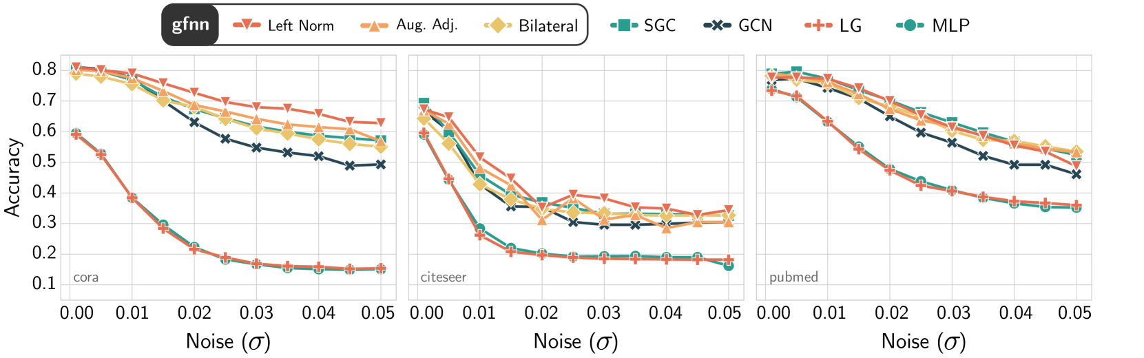
7.2 Denoising Effect of Graph Filters

For each dataset in Table 1, we introduce a white noise $𝒩(0,{\delta }^2)$ into the feature vectors with $\delta$ in range $(0.01,0.05)$. According to the implications of Theorem 8 and Theorem 7, GCN should exhibit a low tolerance to feature noise due to its first-order denoising nature. As the noise level increases, we see in Figure 4 that GCN, Logistic Regression (LR), and MLP tend to overfit more to noise. On the other hand, gfNN and SGC remain comparably noise tolerant.

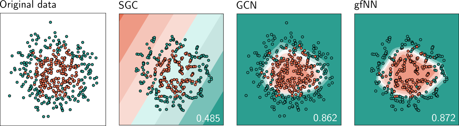
7.3 Expressiveness of Graph Filters

Since graph convolution is simply denoising, we expect it to have little contribution to non-linearity learning. Therefore, we implement a simple 2-D two circles dataset to see whether graph filtering can have the non-linear manifold learning effect. Based on the Euclidean distance between data points, we construct a $k$-nn graph to use as the underlying graph structure. In this particular experiment, we have each data point connected to the 5 closest neighbors. Figure 5 demonstrates how SGC is unable to classify a simple 500-data-points set visually.

Figure 5: Decision boundaries on 500 generated data samples following the two circles pattern

On the other hand, SGC, GCN, and our model gfNN perform comparably on most benchmark graph datasets. Table 2 compares the accuracy (f1-micro for Reddit) of randomized train/test sets. We see that all these graph neural networks have similar performance (some minor improvement might subject to hyperparameters tuning). Therefore, we believe current benchmark datasets for graph neural network have quite “simple” feature spaces.

In practice, both of our analysis and experimental results suggest that the graph convolutional layer should be thought of simply as a denoising filter. In contrast to the recent design trend involving GCN Abu-El-Haija et al. (2019); Valsesia et al. (2019) , our results imply that simply stacking GCN layers might only make the model more prone to feature noise while having the same expressiveness as a simple MLP.

Table 2: Average test accuracy on random train/val/test splits (5 times)

	Denoise	Classifier	Cora	Citeseer	Pubmed	Reddit	PPI	Two Circles
GCN	1st order	Non-linear	$80.0\pm 1.8$	$69.6\pm 1.1$	$79.3\pm 1.3$	OOM	OOM	$83.9\pm 3.1$
SGC	2nd order	Linear	$77.6\pm 2.2$	$65.6\pm 0.1$	$78.4\pm 1.1$	$94.9\pm 1.2$	$62.0\pm 1.2$	$54.5\pm 4.4$
gfNN	2nd order	Non-linear	$80.9\pm 1.3$	$69.3\pm 1.1$	$81.2\pm 1.5$	$92.4\pm 2.2$	$62.2\pm 1.5$	$84.6\pm 2.5$

8 Discussion

There has been little work addressed the limits of the GCN architecture. Kawamoto et al. (2018) took the mean-field approach to analyze a simple GCN model to statistical physics. They concluded that backpropagation improves neither accuracy nor detectability of a GCN-based GNN model. Li et al. (2018) empirically analyzed GCN models with many layers under the limited labeled data setting and stated that GCN would not do well with little labeled data or too many stacked layers. While these results have provided an insightful view for GCN, they have not insufficiently answered the question: When we should we use GNN?.

Our results indicate that we should use the GNN approach to solve a given problem if Assumption 1 holds. From our perspective, GNNs derived from GCN simply perform noise filtering and learn from denoised data. Based on our analysis, we propose two cases where GCN and SGC might fail to perform: noisy features and nonlinear feature spaces. In turn, we propose a simple approach that works well in both cases.

Recently GCN-based GNNs have been applied in many important applications such as point-cloud analysis Valsesia et al. (2019) or weakly-supervised learning Garcia and Bruna (2017). As the input feature space becomes complex, we advocate revisiting the current GCN-based GNNs design. Instead of viewing a GCN layer as the convolutional layer in computer vision, we need to view it simply as a denoising mechanism. Hence, simply stacking GCN layers only introduces overfitting and complexity to the neural network design.

Appendix A Proofs

Proof of Theorem 3.

Since the generalized eigenvalues of $(D+\gamma I,L)$ are the eigenvalues of a positive semidefinite matrix ${(D+\gamma I)}^{1/2}L{(D+\gamma I)}^{1/2}$, these are non-negative real numbers. To obtain the shrinking result, we use the Courant–Fisher–Weyl’s min-max principle [Bhatia, 2013, Corollary III. 1.2]: For any ,

${\lambda }_i({\gamma }_2)$ $=\underset{H:\text{subspace},\dim (H)=i}{\min }\underset{x\in H,x\ne 0}{\max }{\displaystyle \frac{x^{\top }Lx}{x^{\top }(D+{\gamma }_{2}I)x}}$ (13)

$\le \underset{H:\text{subspace},\dim (H)=i}{\min }\underset{x\in H,x\ne 0}{\max }{\displaystyle \frac{x^{\top }Lx}{x^{\top }(D+{\gamma }_{1}I)x}}$ (14)

$={\lambda }_i({\gamma }_1).$ (15)

Here, the second inequality follows because for all $x\ne 0$ Hence, the inequality is strict if $x^{\top }Lx\ne 0$, i.e., ${\lambda }_i({\gamma }_1)\ne 0$. ∎

Lemma 9.

If $X$ has a frequency at most $ϵ$ then ${\mathrm{\Vert }h\mathit{}\mathrm{(}ℒ\mathrm{)}\mathit{}X\mathrm{\Vert }}_D^{\mathrm{2}}\mathrm{\le }{\max }_{t\mathrm{\in }\mathrm{[}\mathrm{0}\mathrm{,}ϵ\mathrm{]}}\mathit{}h\mathit{}\mathrm{(}t\mathrm{)}\mathit{}{\mathrm{\Vert }X\mathrm{\Vert }}_D^{\mathrm{2}}$.

Proof.

By the Parseval identity,

${\Vert ℒX\Vert }_D^2$ $={\displaystyle \sum _{\lambda \in \mathrm{\Lambda }}}h(\lambda ){\Vert \widehat{𝐱}(\lambda )\Vert }_2^2$ (16)

$\le \underset{t\in [0,ϵ]}{\max }h(t){\displaystyle \sum _{\lambda \in \mathrm{\Lambda }}}{\Vert \widehat{𝐱}(\lambda )\Vert }_2^2$ (17)

$=\underset{t\in [0,ϵ]}{\max }h(t){\Vert \widehat{X}\Vert }_2^2$ (18)

$=\underset{t\in [0,ϵ]}{\max }h(t){\Vert \widehat{X}\Vert }_D^2.$ (19)

∎

Proof of Lemma 5.

By substituting $X=\overline{X}+Z$, we obtain

${\Vert \overline{X}-{\tilde{A}}_{\text{rw}}^{k}X\Vert }_{\tilde{D}}$ $\le {\Vert (I-{\tilde{A}}_{\text{rw}}^k)\overline{X}\Vert }_{\tilde{D}}+{\Vert {\tilde{A}}_{\text{rw}}^{k}Z\Vert }_{\tilde{D}}.$ (20)

By Lemma 9, the first term is bounded by $\sqrt{kϵ}{\Vert \overline{X}\Vert }_D$. By the Parseval identity (4), the second term is evaluated by

${\Vert {\tilde{A}}_{\text{rw}}^{k}Z\Vert }_{\tilde{D}}^2$ $={\displaystyle \sum _{\lambda \in \mathrm{\Lambda }}}{(1-\lambda )}^{2k}{\Vert \widehat{𝐳}(\lambda )\Vert }_2^2$ (21)

$={\displaystyle \sum _{\lambda \in \mathrm{\Lambda },p\in \{1,\mathrm{\dots },d\}}}{(1-\lambda )}^{2k}\widehat{z}{(\lambda ,p)}^2$ (22)

By [Laurent and Massart, 2000, Lemma 1], we have

$\mathrm{Prob}\left\{{\displaystyle \sum _{\lambda ,p}}{(1-\lambda )}^{2k}(\widehat{z}{(\lambda ,p)}^2/{\sigma }^2-1)\ge 2\sqrt{t{\displaystyle \sum _{\lambda ,p}}{(1-\lambda )}^{4k}}+2t\right\}\le e^{-t}.$ (23)

By substituting $t=\log (1/\delta )$ with $\delta \le 1/2$, we obtain

$\mathrm{Prob}\left\{{\displaystyle \sum _{\lambda ,p}}{(1-\lambda )}^{2k}\widehat{z}{(\lambda ,p)}^2\ge 5{\sigma }^{2}nd\log (1/\delta ){\displaystyle \frac{{\sum }_{\lambda }{(1-\lambda )}^{2k}}{n}}\right\}\le 1-\delta .$ (24)

Note that $𝔼[\parallel Z{\parallel }_D^2={\sigma }^{2}nd$, and

${\displaystyle \frac{{\sum }_{\lambda }{(1-\lambda )}^{2k}}{n}}={\displaystyle \frac{\mathrm{tr}({\tilde{A}}_{\text{rw}}^{2k})}{n}}=R(2k)$ (25)

since $(i,j)$ entry of ${\tilde{A}}_{\text{rw}}^{2k}$ is the probability that a random walk starting from $i\in 𝒱$ is on $j\in 𝒱$ at $2k$ step, we obtain the lemma. ∎

Proof of Theorem 7.

By the Lipschitz continuity of $\sigma$, we have

$\parallel h_{\text{MLP}}(\overline{X}|W_1,W_2)-h_{\text{MLP}}({\tilde{A}}_{\text{rw}}^{k}X|W_1,W_2){\parallel }_D$ $\le {\Vert \overline{X}-{\tilde{A}}_{\text{rw}}^{k}X\Vert }_D\rho (W_1)\rho (W_2).$ (26)

By using Lemma 5, we obtain the result. ∎

Lemma 10.

If $X$ has a frequency at most $ϵ$ then there exists $Y$ such that $Y$ has a frequency at most $\sqrt{ϵ}$ and ${\mathrm{\Vert }\sigma \mathit{}\mathrm{(}X\mathrm{)}\mathrm{-}Y\mathrm{\Vert }}_D^{\mathrm{2}}\mathrm{\le }\sqrt{ϵ}\mathit{}{\mathrm{\Vert }X\mathrm{\Vert }}_D^{\mathrm{2}}$.

Proof.

We choose $Y$ by truncating the frequency components greater than $\sqrt{ϵ}$. Then,

${\Vert \sigma (X)-Y\Vert }_D^2$ $={\displaystyle \sum _{\lambda >\sqrt{ϵ}}}{\Vert \widehat{\sigma (X)}(\lambda )\Vert }^2$ (27)

$\le {\displaystyle \frac{1}{\sqrt{ϵ}}}{\displaystyle \sum _{\lambda }}\lambda {\Vert \widehat{\sigma (X)}(\lambda )\Vert }^2$ (28)

$={\displaystyle \frac{1}{\sqrt{ϵ}}}{\displaystyle \sum _{(u,v)\in E}}{\Vert \sigma (x(u))-\sigma (x(v))\Vert }_2^2$ (29)

$\le {\displaystyle \frac{1}{\sqrt{ϵ}}}{\displaystyle \sum _{(u,v)\in E}}{\Vert x(u)-x(v)\Vert }_2^2$ (30)

$=\sqrt{ϵ}{\displaystyle \sum _{\lambda }}\lambda {\Vert \widehat{x}(\lambda )\Vert }_2^2$ (31)

$\le \sqrt{ϵ}{\displaystyle \sum _{\lambda }}{\Vert \widehat{x}(\lambda )\Vert }_2^2$ (32)

$=\sqrt{ϵ}{\Vert X\Vert }_D^2.$ (33)

∎

Proof of Theorem 8.

${\Vert \sigma (\overline{X}{W}_1)W_2-{\tilde{A}}_{\text{rw}}\sigma ({\tilde{A}}_{\text{rw}}X{W}_1)W_2\Vert }_D$ (34)

$\le \left({\Vert \sigma (\overline{X}{W}_1)-{\tilde{A}}_{\text{rw}}\sigma (\overline{X}{W}_1)\Vert }_D+{\Vert {\tilde{A}}_{\text{rw}}\sigma (\overline{X}{W}_1)-{\tilde{A}}_{\text{rw}}\sigma ({\tilde{A}}_{\text{rw}}X{W}_1)\Vert }_D\right)\rho (W_2)$ (35)

$=\left({\Vert {\tilde{L}}_{\text{rw}}\sigma (\overline{X}{W}_1)\Vert }_D+{\Vert \overline{X}-{\tilde{A}}_{\text{rw}}X\Vert }_D\rho (W_1)\right)\rho (W_2)$ (36)

$\le \left(O({ϵ}^{1/4}){\Vert \overline{X}\Vert }_D+R(2){\Vert Z\Vert }_D\right)\rho (W_1)\rho (W_2).$ (37)

∎

References

- Abu-El-Haija et al. [2019] Sami Abu-El-Haija, Bryan Perozzi, Amol Kapoor, Hrayr Harutyunyan, Nazanin Alipourfard, Kristina Lerman, Greg Ver Steeg, and Aram Galstyan. Mixhop: Higher-order graph convolution architectures via sparsified neighborhood mixing. In Proceedings of the 36th International Conference on International Conference on Machine Learning, volume 97. JMLR, 2019.
- Bastings et al. [2017] Joost Bastings, Ivan Titov, Wilker Aziz, Diego Marcheggiani, and Khalil Sima’an. Graph convolutional encoders for syntax-aware neural machine translation. Empirical Methods in Natural Language Processing, 2017.
- Belkin and Niyogi [2004] Mikhail Belkin and Partha Niyogi. Semi-supervised learning on riemannian manifolds. Machine Learning, 56(1-3):209–239, 2004.
- Bhatia [2013] Rajendra Bhatia. Matrix analysis, volume 169. Springer Science & Business Media, 2013.
- Chung [1997] Fan R.K. Chung. Spectral graph theory. American Mathematical Society, 1997.
- Defferrard et al. [2016] Michaël Defferrard, Xavier Bresson, and Pierre Vandergheynst. Convolutional neural networks on graphs with fast localized spectral filtering. In Advances in neural information processing systems, pages 3844–3852, 2016.
- Dembo et al. [2013] Amir Dembo, Andrea Montanari, and Nike Sun. Factor models on locally tree-like graphs. The Annals of Probability, 41(6):4162–4213, 2013.
- Fout et al. [2017] Alex Fout, Jonathon Byrd, Basir Shariat, and Asa Ben-Hur. Protein interface prediction using graph convolutional networks. In Advances in Neural Information Processing Systems, pages 6530–6539, 2017.
- Garcia and Bruna [2017] Victor Garcia and Joan Bruna. Few-shot learning with graph neural networks. International Conference on Learning Representations, 2017.
- Gilmer et al. [2017] Justin Gilmer, Samuel S. Schoenholz, Patrick F. Riley, Oriol Vinyals, and George E. Dahl. Neural message passing for quantum chemistry. In Proceedings of the 34th International Conference on Machine Learning, volume 70, pages 1263–1272. JMLR, 2017.
- Girault et al. [2018] Benjamin Girault, Antonio Ortega, and Shrikanth S. Narayanan. Irregularity-aware graph fourier transforms. IEEE Transactions on Signal Processing, 66(21):5746–5761, 2018.
- Hamilton et al. [2017] Will Hamilton, Zhitao Ying, and Jure Leskovec. Inductive representation learning on large graphs. In Advances in Neural Information Processing Systems, pages 1024–1034, 2017.
- Higham [2008] Nicholas J. Higham. Functions of matrices: theory and computation, volume 104. SIAM, 2008.
- Kawamoto et al. [2018] Tatsuro Kawamoto, Masashi Tsubaki, and Tomoyuki Obuchi. Mean-field theory of graph neural networks in graph partitioning. In Advances in Neural Information Processing Systems, pages 4361–4371, 2018.
- Kingma and Ba [2015] Diederik P. Kingma and Jimmy Ba. Adam: A method for stochastic optimization. International Conference on Learning Representations, 2015.
- Kipf and Welling [2017] Thomas N. Kipf and Max Welling. Semi-supervised classification with graph convolutional networks. In International Conference on Learning Representations, 2017.
- Laurent and Massart [2000] Beatrice Laurent and Pascal Massart. Adaptive estimation of a quadratic functional by model selection. Annals of Statistics, pages 1302–1338, 2000.
- Li et al. [2018] Qimai Li, Zhichao Han, and Xiao-Ming Wu. Deeper insights into graph convolutional networks for semi-supervised learning. In Thirty-Second AAAI Conference on Artificial Intelligence, 2018.
- Ortega et al. [2018] Antonio Ortega, Pascal Frossard, Jelena Kovačević, José MF Moura, and Pierre Vandergheynst. Graph signal processing: Overview, challenges, and applications. Proceedings of the IEEE, 106(5):808–828, 2018.
- Rabiner and Gold [1975] Lawrence R. Rabiner and Bernard Gold. Theory and application of digital signal processing. Englewood Cliffs, NJ, Prentice-Hall, Inc., 1975.
- Santoro et al. [2017] Adam Santoro, David Raposo, David G. Barrett, Mateusz Malinowski, Razvan Pascanu, Peter Battaglia, and Timothy Lillicrap. A simple neural network module for relational reasoning. In Advances in Neural Information Processing Systems, pages 4967–4976, 2017.
- Sen et al. [2008] Prithviraj Sen, Galileo Namata, Mustafa Bilgic, Lise Getoor, Brian Galligher, and Tina Eliassi-Rad. Collective classification in network data. AI magazine, 29(3):93–93, 2008.
- Shuman et al. [2012] David I. Shuman, Sunil K. Narang, Pascal Frossard, Antonio Ortega, and Pierre Vandergheynst. The emerging field of signal processing on graphs: Extending high-dimensional data analysis to networks and other irregular domains. arXiv preprint arXiv:1211.0053, 2012.
- Valsesia et al. [2019] Diego Valsesia, Giulia Fracastoro, and Enrico Magli. Learning localized generative models for 3d point clouds via graph convolution. International Conference on Learning Representations, 2019.
- Vaseghi [2008] Saeed V. Vaseghi. Advanced digital signal processing and noise reduction. John Wiley & Sons, 2008.
- Veličković et al. [2017] Petar Veličković, Guillem Cucurull, Arantxa Casanova, Adriana Romero, Pietro Lio, and Yoshua Bengio. Graph attention networks. International Conference on Learning Representations, 2017.
- Veličković et al. [2019] Petar Veličković, William Fedus, William L. Hamilton, Pietro Liò, Yoshua Bengio, and R. Devon Hjelm. Deep graph infomax. International Conference on Learning Representations, 2019.
- Wu et al. [2019] Felix Wu, Tianyi Zhang, Amauri Holanda de Souza Jr., Christopher Fifty, Tao Yu, and Kilian Q. Weinberger. Simplifying graph convolutional networks. In Proceedings of the 36th International Conference on International Conference on Machine Learning, volume 97. JMLR, 2019.
- Xu et al. [2019] Keyulu Xu, Weihua Hu, Jure Leskovec, and Stefanie Jegelka. How powerful are graph neural networks? International Conference on Learning Representations, 2019.
- Yang et al. [2016] Zhilin Yang, William W Cohen, and Ruslan Salakhutdinov. Revisiting semi-supervised learning with graph embeddings. In Proceedings of the 33rd International Conference on International Conference on Machine Learning, volume 48. JMLR, 2016.
- Zhang et al. [2018a] Jiani Zhang, Xingjian Shi, Junyuan Xie, Hao Ma, Irwin King, and Dit-Yan Yeung. Gaan: Gated attention networks for learning on large and spatiotemporal graphs. In Proceedings of the Thirty Fourth Conference on Uncertainty in Artificial Intelligence (UAI), 2018a.
- Zhang et al. [2018b] Yuhao Zhang, Peng Qi, and Christopher D. Manning. Graph convolution over pruned dependency trees improves relation extraction. Empirical Methods in Natural Language Processing, 2018b.
- Zitnik and Leskovec [2017] Marinka Zitnik and Jure Leskovec. Predicting multicellular function through multi-layer tissue networks. Bioinformatics, 33(14):i190–i198, 2017.