Federated Learning Meets Multi-objective Optimization

Abstract

Federated learning has emerged as a promising, massively distributed way to train a joint deep model over large amounts of edge devices while keeping private user data strictly on device. In this work, motivated from ensuring fairness among users and robustness against malicious adversaries, we formulate federated learning as multi-objective optimization and propose a new algorithm FedMGDA+ that is guaranteed to converge to Pareto stationary solutions. FedMGDA+ is simple to implement, has fewer hyperparameters to tune, and refrains from sacrificing the performance of any participating user. We establish the convergence properties of FedMGDA+ and point out its connections to existing approaches. Extensive experiments on a variety of datasets confirm that FedMGDA+ compares favorably against state-of-the-art.

Keywords Pareto optimization, Distributed algorithms, Federated learning, Edge computing, Machine learning, Neural networks.

1 Introduction

Deep learning has achieved impressive successes on a number of domain applications, thanks largely to innovations on algorithmic and architectural design, and equally importantly to the tremendous amount of computational power one can harness through GPUs, computer clusters and dedicated software and hardware. Edge devices, such as smart phones, tablets, routers, car devices, home sensors, etc., due to their ubiquity and moderate computational power, impose new opportunities and challenges for deep learning. On the one hand, edge devices have direct access to privacy sensitive data that users may be reluctant to share (with say data centers), and they are much more powerful than their predecessors, capable of conducting a significant amount of on-device computations. On the other hand, edge devices are largely heterogeneous in terms of capacity, power, data, availability, communication, memory, etc., posing new challenges beyond conventional in-house training of machine learning models. Thus, a new paradigm, known as federated learning (FL) (McMahan et al.,, 2017) that aims at harvesting the prospects of edge devices, has recently emerged. Developing new FL algorithms and systems on edge devices has since become a hot research topic in machine learning.

From the beginning of its birth, FL has close ties to conventional distributed optimization. However, FL emerged from the pressing need to address news challenges in the mobile era that existing distributed optimization algorithms were not designed for per se. We mention the following characteristics of FL that are most relevant to our work, and refer to the excellent surveys (Li et al.,, 2019; Yang et al.,, 2019; Kairouz et al.,, 2019) and the references therein for more challenges and applications in FL.

• Non-IID: Each user’s data can be distinctively different from every other user’s, violating the standard iid assumption in statistical learning and posing significant difficulty in formulating the goal in precise mathematical terms (Mohri et al.,, 2019). The distribution of user data is often severely unbalanced.

• Limited communication: Communication between each user and a central server is constrained by network bandwidth, device status, user participation incentive, etc., demanding a thoughtful balance between computation (on each user device) and communication.

• Privacy: Protecting user (data) privacy is of uttermost importance in FL. It is thus not possible to share user data (even to a cloud arbitrator), which adds another layer of difficulty in addressing the previous two challenges.

• Fairness: As argued forcibly in recent work (e.g., Mohri et al., 2019; Li et al., 2020b ), ensuring fairness among users has become another serious goal in FL, as it largely determines users’ willingness to participate and ensures some degree of robustness against malicious user manipulations.

• Robustness: FL algorithms are eventually deployed in the wild hence subject to malicious attacks. Indeed, adversarial attacks (e.g., Bagdasaryan et al., 2020; Sun et al., 2019; Bhagoji et al., 2019) have been constructed recently to reveal vulnerabilities of FL systems against malicious manipulations at the user side.

In this work, motivated from the last two challenges above, i.e.fairness and robustness, we propose a new algorithm FedMGDA+ that complements and improves existing FL systems. FedMGDA+ is based on multi-objective optimization and is guaranteed to converge to Pareto stationary solutions. FedMGDA+ is simple to implement, has fewer hyperparameters to tune, and most importantly refrains from sacrificing the performance of any participating user. We demonstrate the superior performance of FedMGDA+ under a variety of metrics including accuracy, fairness, and robustness.

We summarize our contributions as follows:

• In §3, based on the proximal average we provide a novel, unifying and revealing interpretation of existing FL practices.

• In §4, we summarize some background on multi-objective optimization and point out its connections to existing FL algorithms. We believe this new perspective will yield more fruitful exchanges between the two fields in the future.

• In §5, we propose FedMGDA+ that complements existing FL systems while taking robustness and fairness explicitly into its algorithmic design. We prove that FedMGDA+ converges to a Pareto stationary solution under mild assumptions.

• In §6, we perform extensive experiments to validate the competitiveness of FedMGDA+ under a variety of desirable metrics, and to illustrate the respective pros and cons of our and alternative algorithms.

We discuss more related work in §2 and we conclude in §7 with some future directions.

To facilitate reproducibility, we have released our code at: https://github.com/watml/Fed-MGDA.

2 Related Work

In this section we give a brief review of some recent work that is directly related to ours and put our contributions in context. To start with, McMahan et al., (2017) proposed the first FL algorithm known as “Federated Averaging” (a.k.a., FedAvg), which is a synchronous update scheme that proceeds in several rounds. At each round, the central server sends the current global model to a subset of users, each of which then uses its respective local data to update the received model. Upon receiving the updated local models from users, the server performs aggregation, such as simple averaging, to update the global model. For more discussion on different averaging schemes, see Li et al., (2020). Li et al., 2020a extended FedAvg to better deal with non-i.i.d. distribution of data, by adding a “proximal regularizer” to the local loss functions and minimizing the Moreau envelope function for each user. The resulting algorithm FedProx, as pointed out in §3, is a randomized version of the proximal average algorithm in Yu, (2013) and reduces to FedAvg when regularization diminishes.

Analysing FedAvg has been a challenging task due to its flexible updating scheme, partial user participation, and non-iid distribution of client data Li et al., 2020a . The first theoretical analysis of FedAvg for strongly convex and smooth problems with iid and non-iid data appeared in Stich, (2019) and Li et al., (2020), respectively, where the effect of different sampling and averaging schemes on the convergence rate of FedAvg was also investigated, leading to the conclusion that such effect becomes particularly important when the dataset is unbalanced and non-iid distributed. In Huo et al., (2020), FedAvg was analyzed for non-convex problems, where FedAvg was formulated as a stochastic gradient-based algorithm with biased gradients, and the convergence of FedAvg with decaying step sizes to stationary points was proved. Moreover, Huo et al., (2020) proposed FedMom, a server-side acceleration based on Nesterov’s momentum, and proved again its convergence to stationary points. Lately, Reddi et al., (2020) proposed and analyzed federated versions of several popular adaptive optimizers (e.g. ADAM). They generalize the framework of FedAvg by decoupling the FL update scheme into server optimizer and client optimizer. Interestingly, same as us, Reddi et al., (2020) also observed the importance of learning rate decays on both clients and server.

Recently, an interesting work by Pathak and Wainwright, (2020) demonstrated theoretically that fixed points reached by FedAvg and FedProx (if exist) need not be stationary points of the original optimization problem, even in convex settings and with deterministic updates. To address this issue, they proposed FedSplit to restore the correct fixed points. It still remains open, though, if FedSplit can still converge to the correct fixed points under asynchronous and stochastic user updates, both of which are widely adopted in practice and studied here.

Ensuring fairness among users has become a serious goal in FL since it largely determines users’ willingness to participate in the training process. Mohri et al., (2019) argued that existing FL algorithms can lead to federated models that are biased toward different users. To solve this issue, Mohri et al., (2019) proposed agnostic federated learning (AFL) to improve fairness among users. AFL considers the target distribution as a weighted combination of the user distributions and optimizes the centralized model for the worse-case realization, leading to a saddle-point optimization problem which was solved by a fast stochastic optimization algorithm. On the other hand, based on fair resource allocation in wireless networks, Li et al., 2020b proposed q-fair federated learning (q-FFL) to achieve more uniform test accuracy across users. Li et al., 2020b further proposed q-FedAvg as a communication efficient algorithm to solve q-FFL. However, both AFL and q-FedAvg do not explicitly encourage user participation and they suffer from adversarial attacks while our algorithm FedMGDA+ is designed to be fair among participants and robust against both additive and multiplicative attacks.

FedAvg relies on a coordinate-wise averaging of local models to update the global model. According to Wang et al., 2020b , in neural network (NN) based models, such coordinate-wise averaging might lead to sub-optimal results due to the permutation invariance of NN parameters. To address this issue, Yurochkin et al., (2019) proposed probabilistic federated neural matching (PFNM), which is only applicable to fully connected feed-forward networks. The recent work (Wang et al., 2020b, ) proposed federated matched averaging (FedMA) as a layer-wise extension of PFNM to accommodate CNNs and LSTMs. However, the Bayesian non-parametric mechanism in PFNM and FedMA may be vulnerable to model poisoning attack (Bagdasaryan et al.,, 2020; Bhagoji et al.,, 2019; Wang et al., 2020a, ), while some simple defences, such as norm thresholding and differential privacy, were discussed in Sun et al., (2019). We note that these ideas are complementary to FedMGDA+ and we plan to investigate possible integrations of them in future work.

Lastly, we note that there is significant interest in standardizing the benchmarks, protocols and evaluations in FL, see for instance (Caldas et al.,, 2018; He et al.,, 2020). We have spent significant efforts in adhering to the suggested rules there, by reporting on common datasets, open sourcing our code and including all experimental details.

3 Problem Setup

We recall the federated learning (FL) framework of McMahan et al., (2017) and point out a simple interpretation that seemingly unifies different implementations. We consider FL with $m$ users (edge devices), where the $i$-th user is interested in minimizing a function $f_i:{ℝ}^d\to ℝ,i=1,\mathrm{\dots },m$, defined on a shared model parameter $𝐰\in {ℝ}^d$. Typically, each user function $f_i$ also depends on the respective user’s local (private) data ${𝒟}_i$. The main goal in FL is to collectively and efficiently optimize individual objectives $\{f_i\}$ while meeting challenges such as those mentioned in the Introduction (§1): non-iid distribution of user data, limited communication, user privacy, fairness, robustness, etc..

McMahan et al., (2017) proposed FedAvg to optimize the arithmetic average of individual user functions:

$\underset{𝐰\in {ℝ}^d}{\min }{𝖠}_{𝐟,𝝀}^0(𝐰),\text{where}{𝖠}_{𝐟,𝝀}^0(𝐰):={\displaystyle \sum _{i=1}^m}{\lambda }_i{f}_i(𝐰).$ (1)

The weights ${\lambda }_i$ need to be specified beforehand. Typical choices include the dataset size at each user, the “importance” of each user, or simply uniform, i.e.${\lambda }_i\equiv 1/m$. FedAvg works as follows: At each round, a (random) subset of users is selected, each of which performs $k$ epochs of local (full or minibatch) gradient descent:

$\text{for all}i\text{in parallel},{𝐰}^i\leftarrow {𝐰}^i-\eta \nabla f_i({𝐰}^i),$ (2)

and then the weights are averaged at the server side:

$𝐰\leftarrow {\displaystyle \sum _i}{\lambda }_i{𝐰}^i,$ (3)

which is finally broadcast to the users in the next round. The number of local epochs $k$ turns out to be a key factor. Setting $k=1$ amounts to solving (1) by the usual gradient descent algorithm, while setting $k=\mathrm{\infty }$ (and assuming convergence for each local function $f_i$) amounts to (repeatedly) averaging the respective minimizers of $f_i$’s. We now give a new interpretation of FedAvg that yields insights on what it optimizes with an intermediate $k$.

Our interpretation is based on the proximal average (Bauschke et al.,, 2008). Recall that the Moreau envelope and proximal map of a convex function $f$ is defined respectively as:

${𝖬}_f^{\eta }(𝐰)$ $=\underset{𝐱}{\min }\frac{1}{2\eta }{\Vert 𝐱-𝐰\Vert }_2^2+f(𝐱),$ (4)

${𝖯}_f^{\eta }(𝐰)$ $=\underset{𝐱}{\text{argmin}}\frac{1}{2\eta }{\Vert 𝐱-𝐰\Vert }_2^2+f(𝐱).$ (5)

Given a set of convex functions $𝐟=(f_1,\mathrm{\dots },f_m)$ and positive weights $𝝀=({\lambda }_1,\mathrm{\dots },{\lambda }_m)$ that sum to 1, we define the proximal average as the unique function ${𝖠}_{𝐟,𝝀}^{\eta }$ such that ${𝖯}_{{𝖠}_{𝐟,𝝀}^{\eta }}^{\eta }={\sum }_i{\lambda }_i{𝖯}_{f_i}^{\eta }.$ In other words, the proximal map of the proximal average is the average of proximal maps. More concretely, Bauschke et al., (2008) gave the following explicit, albeit complicated, formula for the proximal average:

${𝖠}_{𝐟,𝝀}^{\eta }(𝐰)$ $=\underset{{𝐰}_1,\mathrm{\dots },{𝐰}_m}{\min }{\displaystyle \sum _{i=1}^m}{\lambda }_i\left[f_i({𝐰}_i)+\frac{1}{2\eta }{\Vert {𝐰}_i\Vert }_2^2\right]-\frac{1}{2\eta }{\Vert 𝐰\Vert }_2^2,$ (6)

$\text{s.t.}{\displaystyle \sum _{i=1}^m}{\lambda }_i{𝐰}_i=𝐰.$ (7)

From the above formula we can easily derive that

${𝖠}_{𝐟,𝝀}^0(𝐰)$ $:=\underset{\eta \to 0+}{lim}{𝖠}_{𝐟,𝝀}^{\eta }(𝐰)={\displaystyle {\sum }_i}{\lambda }_i{f}_i(𝐰),$

${𝖠}_{𝐟,𝝀}^{\mathrm{\infty }}(𝐰)$ $:=\underset{\eta \to \mathrm{\infty }}{lim}{𝖠}_{𝐟,𝝀}^{\eta }(𝐰)=\underset{{\sum }_i{\lambda }_i{𝐰}_i=𝐰}{\min }{\displaystyle {\sum }_i}{\lambda }_i{f}_i({𝐰}_i).$

Interestingly, we can now interpret FedAvg in two extreme settings as minimizing the proximal average:

• FedAvg with $k=1$ local step is exactly the same as minimizing the proximal average ${𝖠}_{𝐟,𝝀}^0(𝐰)$ with $\eta =0$. This is clear from the objective (1) of FedAvg (as our notation already suggests).

• FedAvg with $k=\mathrm{\infty }$ local steps is exactly the same as minimizing the proximal average ${𝖠}_{𝐟,𝝀}^{\mathrm{\infty }}(𝐰)$ with $\eta =\mathrm{\infty }$. Indeed,

  $\left\{\underset{𝐰}{\min }{𝖠}_{𝐟,𝝀}^{\mathrm{\infty }}(𝐰)\right\}=\underset{{𝐰}_1,\mathrm{\dots },{𝐰}_m}{\min }{\displaystyle \sum _i}{\lambda }_i{f}_i({𝐰}_i),$ (8)

  where the right-hand side decouples and hence ${𝐰}_i$ at optimality is a minimizer of $f_i$ (recall that $𝝀\ge 0$).

Therefore, we may interpret FedAvg with an intermediate $k$ as minimizing ${𝖠}_{𝐟,𝝀}^{\eta }$ with an intermediate $\eta$. More interestingly, if we apply the PA-PG algorithm in Yu, (2013, Algo. 222) to minimize ${𝖠}_{𝐟,𝝀}^{\eta }$, we obtain the simple update rule

$𝐰\leftarrow {\displaystyle {\sum }_i}{\lambda }_i{𝖯}_{f_i}^{\eta }(𝐰),$ (9)

where the proximal maps are computed in parallel at the user’s side. We note that the recent FedProx algorithm (Li et al., 2020a, ) is essentially a randomized version of (9). Crucially, we do not need to evaluate the complicated formula (6) as the update (9) only requires its proximal map, which by definition is the average of the individual proximal maps (computed by each user separately). Moreover, the difference between the proximal average ${𝖠}_{𝐟,𝝀}^{\eta }$ and the arithmetic average ${𝖠}_{𝐟,𝝀}^0$ can be uniformly bounded using the Lipschitz constant of each function $f_i$ (Yu,, 2013). Thus, for small step size $\eta$, FedAvg (with any finite $k$) and FedProx all minimize some approximate form of the arithmetic average in (1).

How to set the weights $𝝀$ in FedAvg has been a major challenge. In FL, data is distributed in a highly non-iid and unbalanced fashion, so it is not clear if some chosen arithmetic average in (1) would really satisfy one’s actual intention. A second issue with the arithmetic average in (1) is its well-known non-robustness against malicious manipulations, which has been exploited in recent adversarial attacks (Bhagoji et al.,, 2019). Instead, Agnostic FL (AFL (Mohri et al.,, 2019)) aims to optimize the worst-case loss:

$\underset{𝐰}{\min }\underset{𝝀\in \mathrm{\Lambda }}{\max }{𝖠}_{𝐟,𝝀}^0(𝐰),$ (10)

where the set $\mathrm{\Lambda }$ might cover reality better than any specific $𝝀$ and provide some minimum guarantee for all users (hence achieving mild fairness). On the other hand, the worst-case loss in (10) is perhaps even more non-robust against adversarial attacks. For instance, adding a positive constant to some loss $f_i$ can make it dominate the entire optimization process. The recent work q-FedAvg (Li et al., 2020b, ) proposes an ${\mathrm{\ell }}_q$ norm interpolation between FedAvg (essentially ${\mathrm{\ell }}_1$ norm) and AFL (essentially ${\mathrm{\ell }}_{\mathrm{\infty }}$ norm). By tuning $q$, q-FedAvg can achieve better compromise than FedAvg or AFL.

4 Multi-objective Minimization (MoM)

Multi-objective minimization (MoM) refers to the setting where multiple scalar objective functions, possibly incompatible with each other, need to be minimized simultaneously. It is also called vector optimization (Jahn,, 2009) because the objective functions can be combined into a single vector-valued function. In mathematical terms, MoM can be written as

$\underset{𝐰\in {ℝ}^d}{\min }𝐟(𝐰):=(f_1(𝐰),f_2(𝐰),\mathrm{\dots },f_m(𝐰)),$ (11)

where the minimum is defined wrt the partial ordering:

$𝐟(𝐰)\le 𝐟(𝐳)\iff \forall i=1,\mathrm{\dots },m,f_i(𝐰)\le f_i(𝐳).$ (12)

(We remind that algebraic operations such as $\le$ and $+$, when applied to a vector with another vector or scalar, are always performed component-wise.) Unlike single objective optimization, with multiple objectives it is possible that

$𝐟(𝐰)\nleqq 𝐟(𝐳)\text{and}𝐟(𝐳)\nleqq 𝐟(𝐰),$ (13)

in which case we say $𝐰$ and $𝐳$ are not comparable.

We call ${𝐰}^{\ast }$ a Pareto optimal solution of (11) if its objective value $𝐟({𝐰}^{\ast })$ is a minimum element (wrt the partial ordering in (12)), or equivalently for any $𝐰$, $𝐟(𝐰)\le 𝐟({𝐰}^{\ast })$ implies $𝐟(𝐰)=𝐟({𝐰}^{\ast })$. In other words, it is not possible to improve any component objective in $𝐟({𝐰}^{\ast })$ without compromising some other objective. Similarly, we call ${𝐰}^{\ast }$ a weakly Pareto optimal solution if there does not exist any $𝐰$ such that , i.e., it is not possible to improve all component objectives in $𝐟({𝐰}^{\ast })$. Clearly, any Pareto optimal solution is also weakly Pareto optimal but the converse may not hold.

We point out that the optimal solutions in MoM are usually a set (in general of infinite cardinality) (Mukai,, 1980), and without additional subjective preference information, all Pareto optimal solutions are considered equally good (as they are not comparable against each other). This is fundamentally different from the single objective case.

From now on, for simplicity we assume all objective functions are continuously differentiable but not necessarily convex (to accommodate deep models). Finding a (weakly) Pareto optimal solution in this setting is quite challenging (already so in the single objective case). Instead, we will contend with Pareto stationary solutions, namely those that satisfy an intuitive first order necessary condition:

Definition 1 (Pareto-stationarity, Mukai, 1980).

We call ${𝐰}^{\ast }$ Pareto-stationary iff some convex combination of the gradients $\{\nabla f_i({𝐰}^{\ast })\}$ vanishes, i.e.there exists some $𝛌\ge 0$ such that ${\sum }_i{\lambda }_i=1$ and ${\sum }_i{\lambda }_i\nabla f_i({𝐰}^{\ast })=\mathrm{𝟎}$.

Lemma 1 (Mukai, 1980).

Any Pareto optimal solution is Pareto stationary. Conversely, if all functions are convex, then any Pareto stationary solution is weakly Pareto optimal.

Needless to say, the above results reduce to the familiar ones for the single objective case ($m=1$).

There exist many algorithms for finding Pareto stationary solutions. We briefly review three popular ones that are relevant for us, and refer the reader to the excellent monograph (Miettinen,, 1998) for more details.

Weighted approach. Let $𝝀\in \mathrm{\Delta }$ (the simplex) and consider the following single, weighted objective:

$\underset{𝐰}{\min }{\displaystyle \sum _{i=1}^m}{\lambda }_i{f}_i(𝐰).$ (14)

This is essentially the approach taken by FedAvg, with any (global) minimizer of (14) being weakly Pareto optimal (in fact, Pareto optimal if all weights ${\lambda }_i$ are positive). From Definition 1 it is clear that any stationary solution of the weighted scalar problem (14) is a Pareto stationary solution of the original MoM (11). Note that the scalarization weights $𝝀$, once chosen, are fixed throughout. Different $𝝀$ leads to different Pareto stationary solutions.

$ϵ$-constraint. Let $\mathit{ϵ}\in {ℝ}^{m-1}$, $\iota \in \{1,\mathrm{\dots },m\}$ and consider the following constrained scalar problem:

$\underset{𝐰}{\min }$ $f_{\iota }(𝐰)$ (15)

$\mathrm{s}.\mathrm{t}.$ $f_i(𝐰)\le {ϵ}_i,\forall i\ne \iota .$ (16)

Assuming the constraints are satisfiable, then any (global) minimizer of (15) is again weakly Pareto optimal. The $ϵ$-constraint approach is closely related to the weighted approach above, through the usual Lagrangian reformulation. Both require fixing an $m-1$ dimensional parameter in advance ($𝝀$ vs. $\mathit{ϵ}$), though.

Chebyshev approach. Let $𝐬\in {ℝ}^m$ and consider the minimax problem (where recall that $\mathrm{\Delta }$ is the simplex constraint):

$\underset{𝐰}{\min }\underset{𝝀\in \mathrm{\Delta }}{\max }{𝝀}^{\top }(𝐟(𝐰)-𝐬).$ (17)

Again, any (global) minimizer is weakly Pareto optimal. Here $𝐬$ is a fixed vector that ideally lower bounds $𝐟$. This is essentially the approach taken by AFL (Mohri et al.,, 2019) with $𝐬=\mathrm{𝟎}$.

5 FL as Multi-objective Minimization

Having introduced both FL and MoM, and observed some connections between the two, it is very natural to treat each user function $f_i$ in FL as a separate objective in MoM and aim to optimize them simultaneously as in (11). This will be the main approach we follow below, which, to the best of our knowledge, has not been formally explored before (despite of the apparent connections that we saw in the previous section, perhaps retrospectively). In particular, we will extend the multiple gradient descent algorithm (Mukai,, 1980) in MoM to FL, draw connections to existing FL algorithms, and prove convergence properties of our extended algorithm FedMGDA+. Very importantly, the notion of Pareto optimality and stationarity immediately enforces fairness among users, as we are discouraged from improving certain users by sacrificing others.

To further motivate our development, let us compare to the objective in AFL (Mohri et al.,, 2019):

$\underset{𝐰}{\min }\underset{𝝀\in \mathrm{\Delta }}{\max }{𝝀}^{\top }𝐟(𝐰)\equiv \underset{𝐰}{\min }\underset{i=1,\mathrm{\dots },m}{\max }{f}_i(𝐰),$ (18)

where $\mathrm{\Delta }$ denotes the simplex. By optimizing the worst loss than the average loss in FedAvg, AFL provides some guarantee to all users hence achieving some form of fairness. However, note that AFL’s objective (18) is not robust against adversarial attacks. In fact, if a malicious user artificially “inflates” its loss $f_i$ (e.g., even by adding/multiplying a constant), it can completely dominate and mislead AFL to solely focus on optimizing its performance. The same issue applies to q-FedAvg (Li et al., 2020b, ), albeit with a less dramatic effect if $q$ is small.

AFL’s objective (18) is very similar to the Chebyshev approach in MoM (see Section 4), which inspires us to propose the following iterative algorithm for solving (11):

${\widetilde{𝐰}}_{t+1}=\underset{𝐰}{\text{argmin}}\underset{𝝀\in \mathrm{\Delta }}{\max }{𝝀}^{\top }(𝐟(𝐰)-𝐟({\widetilde{𝐰}}_t)),$ (19)

where we adaptively “center” the user functions using function values from the previous iteration. When the functions $f_i$ are smooth, we apply the quadratic bound to obtain:

${𝐰}_{t+1}=\underset{𝐰}{\text{argmin}}\underset{𝝀\in \mathrm{\Delta }}{\max }{𝝀}^{\top }{J}_{𝐟}^{\top }({𝐰}_t)(𝐰-{𝐰}_t)+\frac{1}{2\mathrm{\eta }}{\Vert 𝐰-{𝐰}_t\Vert }^2,$ (20)

where $J_{𝐟}=[\nabla f_1,\mathrm{\dots },\nabla f_m]\in {ℝ}^{d\times m}$ is the Jacobian and $\mathrm{\eta }>0$ is the step size. Crucially, note that $𝐟({𝐰}_t)$ does not appear in the above bound (20) since we subtracted it off in (19). Since (20) is convex in $𝐰$ and concave in $𝝀$ we can swap min with max and obtain the dual:

$\underset{𝝀\in \mathrm{\Delta }}{\max }$ $\underset{𝐰}{\min }{𝝀}^{\top }{J}_{𝐟}^{\top }({𝐰}_t)(𝐰-{𝐰}_t)+\frac{1}{2\mathrm{\eta }}{\Vert 𝐰-{𝐰}_t\Vert }^2.$ (21)

Solving $𝐰$ by setting its derivative to $\mathrm{𝟎}$ we arrive at:

${𝐰}_{t+1}={𝐰}_t-\mathrm{\eta }{𝐝}_t,{𝐝}_t=J_{𝐟}({𝐰}_t){𝝀}_t^{\ast },$ (22)

$\text{where}{𝝀}_t^{\ast }=\underset{𝝀\in \mathrm{\Delta }}{\text{argmin}}{\Vert J_{𝐟}({𝐰}_t)𝝀\Vert }^2.$ (23)

Note that ${𝐝}_t$ is precisely the minimum-norm element in the convex hull of the columns (i.e., gradients) in the Jacobian $J_{𝐟}$, and finding ${𝝀}_t^{\ast }$ amounts to solving a simple quadratic program. The resulting iterative algorithm in (22) is known as multiple gradient descent algorithm (MGDA), which has been (re)discovered in Mukai, (1980); Fliege and Svaiter, (2000); Désidéri, (2012) and recently applied to multitask learning in Sener and Koltun, (2018); Lin et al., (2019) and to training GANs in Albuquerque et al., (2019). Our concise derivation here reveals some new insights about MGDA, in particular its connection to AFL.

To adapt MGDA to the federated learning setting, we propose the following extensions.

Balancing user average performance and fairness. We observe that the MGDA update in (22) resembles FedAvg, with the crucial difference that MGDA automatically tunes the dual weighting variable $𝝀$ in each step while FedAvg pre-sets $𝝀$ based on a priori information about the user functions (or simply uniform in lack of such information). Importantly, the direction ${𝐝}_t$ found in MGDA is a common descent direction for all participating objectives:

$𝐟({𝐰}_{t+1})$ $\le 𝐟({𝐰}_t)+J_{𝐟}^{\top }({𝐰}_t)({𝐰}_{t+1}-{𝐰}_t)+\frac{1}{2\mathrm{\eta }}{\Vert {𝐰}_{t+1}-{𝐰}_t\Vert }^2$

$\le 𝐟({𝐰}_t),$ (24)

where the first inequality follows from familiar smoothness assumption on $𝐟$ while the second inequality follows simply from plugging $𝐰={𝐰}_t$ in (20) and noting that ${𝐰}_{t+1}$ by definition can only decrease (20) even more. It is clear that equality is attained iff ${𝐝}_t=J_{𝐟}({𝐰}_t){𝝀}_t^{\ast }=\mathrm{𝟎}$, i.e., ${𝐰}_t$ is Pareto-stationary (see Section 4). In other words, MGDA never sacrifices any participating objective to trade for more sizable improvements over some other objective, something FedAvg with a fixed weighting $𝝀$ might attempt to do. On the other hand, FedAvg with a fixed weighting $𝝀$ may achieve higher average performance under the weighting $𝝀$. It is natural to introduce the following trade-off between average performance and fairness:

$\text{update (}\text{<a class="ltx\_ref" href="\#S5.E22" title="Equation 22 ‣ 5 FL as Multi-objective Minimization ‣ Federated Learning Meets Multi-objective Optimization"><span class="ltx\_text ltx\_ref\_tag">22</span></a>}\text{) with}{𝝀}_t^{\ast }=\underset{𝝀\in \mathrm{\Delta },{\Vert 𝝀-{𝝀}_0\Vert }_{\mathrm{\infty }}\le ϵ}{\text{argmin}}{\Vert J_{𝐟}({𝐰}_t)𝝀\Vert }^2.$ (25)

Clearly, setting $ϵ=0$ recovers FedAvg with a priori weighting ${𝝀}_0$ while setting $ϵ=1$ recovers MGDA where the weighting variable $𝝀$ is tuned without any restriction to achieve maximal fairness. In practice, with an intermediate $ϵ\in (0,1)$ we may strike a desirable balance between the two (sometimes) conflicting goals. Moreover, even with the uninformative weighting ${𝝀}_0=\mathrm{𝟏}/m$, using an intermediate $ϵ$ allows us to upper bound the contribution of each user function to the common direction ${𝐝}_t$ hence achieve some form of robustness against malicious manipulations.

Robustness against malicious users through normalization. Existing work (e.g., Bhagoji et al.,, 2019; Xie et al.,, 2019) has demonstrated that the average gradient in FedAvg can be easily manipulated by even a single malicious user. While more robust aggregation strategies are studied recently (see e.g., Blanchard et al.,, 2017; Yin et al.,, 2018; Diakonikolas et al.,, 2019), they do not necessarily maintain the convergence properties of FedMGDA+ (e.g.finding a common descent direction and converging to a Pareto stationary solution). Instead, we propose to simply normalize the gradients from each user to unit length, based on the following considerations: (a) Normalizing the (sub)gradient is common for specialists in nonsmooth and stochastic optimization (Anstreicher and Wolsey,, 2009) and sometimes eases step size tuning. (b) Solving the weights ${𝝀}_t^{\ast }$ in (22) with normalized gradients still guarantees fairness, i.e., the resulting direction ${𝐝}_t$ is descending for all participating objectives (by a completely similar reasoning as the remark after (5)). (c) Normalization restores robustness against multiplicative “inflation” from any malicious user, which, combined with MGDA’s built-in robustness against additive “inflation” (see Equation 19), offers reasonable robustness guarantees against adversarial attacks.

Balancing communication and on-device computation. Communication between user devices and the central server is heavily constrained in FL, due to a variety of reasons mentioned in §3. On the other hand, modern edge devices are capable of performing reasonable amount of on-device computations. Thus, we allow each user device to perform multiple local updates before communicating its update $𝐠={𝐰}^0-{𝐰}^{\mathrm{■}}$, namely the difference between the initial ${𝐰}^0$ and the final ${𝐰}^{\mathrm{■}}$, to the central server. The server then calls the (extended) MGDA to perform a global update, which will be broadcast to the next round of user devices. We note that similar strategy was already adopted in many existing FL systems (e.g., McMahan et al.,, 2017; Li et al., 2020b, ; Li et al., 2020a, ).

Subsampling to alleviate non-iid and enhance throughput. Due to the massive number of edge devices in FL, it is not realistic to expect most devices to participate at each or even most rounds. Consequently, the current practice in FL is to select a (different) subset of user devices to participate in each round (McMahan et al.,, 2017). Moreover, randomly subsampling user devices can also help combat the non-iid distribution of user-specific data (e.g., McMahan et al.,, 2017; Li et al.,, 2020). Here we point out an important advantage of our MGDA-based algorithm: its update is along a common descending direction (see (5)), meaning that the objective of any participating user can only decrease. We believe this unique property of MGDA provides strong incentive for users to participate in FL. To our best knowledge, existing FL algorithms do not provide similar algorithmic incentives. Last but not the least, subsampling also solves a degeneracy issue in MGDA: when the number of participating users exceeds the dimension $d$, the Jacobian $J_{𝐟}$ has full row-rank hence (22) achieves Pareto-stationarity in a single iteration and stops making progress. Subsampling removes this undesirable effect and allows different subsets of users to be continuously optimized.

With the above extensions, we summarize our extended algorithm FedMGDA+ in Algorithm 1, and we prove the following convergence guarantees (precise statements and proofs can be found in Appendix A):

Theorem 1a.

Let each user function $f_i$ be $L$-Lipschitz smooth and $M$-Lipschitz continuous, and choose step size ${\mathrm{\eta }}_t$ so that ${\sum }_t{\mathrm{\eta }}_t=\mathrm{\infty }$ and , where ${\sigma }_t^2:=𝐄{\Vert {𝐝}_t-{\widehat{𝐝}}_t\Vert }^2$ with

${𝐝}_t$ $:=J_{𝐟}({𝐰}_t){𝝀}_t,{𝝀}_t=\underset{𝝀\in \mathrm{\Delta }}{\text{argmin}}\Vert J_{𝐟}({𝐰}_t)𝝀\Vert ,$ (26)

${\widehat{𝐝}}_t$ $:={\widehat{J}}_{𝐟}({𝐰}_t){\widehat{𝝀}}_t,{\widehat{𝝀}}_t=\underset{𝝀\in \mathrm{\Delta }}{\text{argmin}}\Vert {\widehat{J}}_{𝐟}({𝐰}_t)𝝀\Vert .$ (27)

Then, with $k=r=1$ we have:

$\underset{t=0,\mathrm{\dots },T}{\min }𝐄{\Vert J_{𝐟}({𝐰}_t){𝝀}_t\Vert }^2\to 0.$ (28)

Here $k$ is the number of local updates and $r$ is the number of minibatches in each local update. The convergence rate depends on how quickly the “variance” term ${\sigma }_t$ of the stochastic common descent direction ${\widehat{d}}_t$ diminishes (if at all), which in turn depends on how aggressively we subsample users or how heterogeneous the users are.

For deterministic gradient updates, we can prove convergence even with more local updates (i.e.$k>1$):

Theorem 1b.

Let each user function $f_i$ be $L$-Lipschitz smooth and $M$-Lipschitz continuous. For any number of local updates $k$, if the global step size ${\mathrm{\eta }}_t\to 0$ with ${\sum }_t{\mathrm{\eta }}_t=\mathrm{\infty }$, local learning rate ${\eta }_t^l\to 0$ and ${\epsilon }_t:=\Vert {𝛌}_t-{\widehat{𝛌}}_t\Vert \to 0$, then we have:

$\underset{t=0,\mathrm{\dots },T}{\min }{\Vert J_{𝐟}({𝐰}_t){𝝀}_t\Vert }^2\to 0.$ (29)

Please refer to Appendix A for the precise statement of the theorem and its proof. We note that one natural approach to bound the deviation ${\epsilon }_t$ is by applying the $ϵ$-constrained version of FedMGDA. For example, if ${\Vert 𝝀-{𝝀}_0\Vert }_{\mathrm{\infty }}\le {ϵ}_t$, and ${ϵ}_t$ is bounded, then ${\epsilon }_t\le 2\sqrt{m}{ϵ}_t$ is also bounded. Thus, ${\epsilon }_t\to 0$ when ${ϵ}_t\to 0$. Moreover, when $k=1$, we do not need the local learning rate ${\eta }_t^l$ to decay for convergence; in addition, if ${\epsilon }_t\equiv 0$ (e.g. in FedAvg), then our convergence guarantee reduces to the usual one for gradient descent, which is expected since we know FedAvg with $k=1,r=1$ is the same as centralized gradient descent. Lastly, we note that when $k>1$, local learning rate ${\eta }_t^l$ must vanish in order to obtain convergence. This importance of local learning rate decay is also pointed out in Reddi et al., (2020).

When the functions $f_i$ are convex, we can derive a finer result:

Theorem 2.

Suppose each user function $f_i$ is convex and $M$-Lipschitz continuous. Suppose at each round FedMGDA+ includes a strongly convex user function whose weight is bounded away from 0. Then, with the choice ${\mathrm{\eta }}_t=\frac{2}{c(t+2)}$ and $k=r=1$, we have

$𝐄{\Vert {𝐰}_t-{𝐰}_t^{\ast }\Vert }^2\le \frac{4M^2}{c^2(t+3)},$ (30)

and ${𝐰}_t-{𝐰}_t^{\ast }\to 0$ almost surely, where ${𝐰}_t^{\ast }$ is the nearest Pareto stationary solution to ${𝐰}_t$ and $c$ is some constant.

A slightly stronger result where we also allow some user functions to be nonconvex can be found in Appendix A. The same results hold if the gradient normalization is bounded away from 0 (otherwise we are already close to Pareto stationarity). For $r,k>1$, using a similar argument as in §3, we expect FedMGDA+ to optimize some proxy problem (such as the proximal average), and we leave the thorough theoretical analysis for future work.

We remark that convergence rate for MGDA, even when restricted to the deterministic case, was only derived recently in Fliege et al., (2019). The stochastic case (that we consider here) is much more challenging and our theorems provide one of the first convergence guarantees for FedMGDA+. We wish to emphasize that FedMGDA+ is not just an alternative algorithm for FL practitioners; it can be used as a post-processing step to enhance existing FL systems or combined with existing FL algorithms (such as FedProx or q-FedAvg). This is particularly appealing with nonconvex user functions as MGDA is capable of converging to all Pareto stationary points while approaches such as FedAvg do not necessarily enjoy this property even when we enumerate the weighting ${𝝀}_0$ (Miettinen,, 1998). Furthermore, it is possible to find multiple or even enumerate all Pareto optimal solutions (i.e.the Pareto front). For instance, we may run FedMGDA+ multiple times with different random seeds or initializations. As shown by Lin et al., (2019), we could also incorporate additional linear constraints in (22) to encode one’s preference and encourage more diverse solutions. However, these techniques become less effective in higher dimensions (i.e.when the number of users is large) and in communication limited settings. Practically, the server may dynamically adjust the linear constraints in (22) to steer the algorithm to a more desirable Pareto stationary solution.

Lastly, we mention that finding the common descent direction (i.e.Line 6 of Algorithm 1) is a standard quadratic programming (QP) problem that is solved only at the server side. For moderate number of (sampled) users, it suffices to employ a generic QP solver while for large number of users we could also solve $\lambda$ efficiently using for instance the conditional gradient algorithm (Sener and Koltun,, 2018), with per-step complexity proportional to the model dimension and the number of participating users. For our experiments below, we used a generic QP sovler and we observed that this overhead is negligible, resulting almost the same overall running time for FedAvg and FedMGDA.

1 for $t=1,2,\mathrm{\dots }$ do

2 choose a subset $I_t$ of $\lceil pm\rceil$ clients/users

3 for $i\in I_t$ do

4 ${𝐠}_i\leftarrow$ ClientUpdate($i,{𝐰}_t$)

${\overline{𝐠}}_i:={𝐠}_i/\Vert {𝐠}_i\Vert$

// normalize

5

6

7 ${𝝀}^{\ast }\leftarrow {\text{argmin}}_{𝝀\in \mathrm{\Delta },{\Vert 𝝀-{𝝀}_0\Vert }_{\mathrm{\infty }}\le ϵ}{\Vert {\sum }_i{\lambda }_i{\overline{𝐠}}_i\Vert }^2$

${𝐝}_t\leftarrow {\sum }_i{\lambda }_i^{\ast }{\overline{𝐠}}_i$

// common direction

8

9 choose (global) step size ${\mathrm{\eta }}_t$

10 ${𝐰}_{t+1}\leftarrow {𝐰}_t-{\mathrm{\eta }}_t{𝐝}_t$

11

12

13 Function ClientUpdate($i,𝐰$):

14 ${𝐰}^0\leftarrow 𝐰$

15 repeat $k$ epochs

// split local data into $r$ batches

16

17 ${𝒟}_i\to {𝒟}_{i,1}\cup \mathrm{\cdots }\cup {𝒟}_{i,r}$

18 for $j\in \{1,\mathrm{\dots },r\}$ do

19 $𝐰\leftarrow 𝐰-\eta \nabla f_i(𝐰;{𝒟}_{i,j})$

20

21

22 return $𝐠:={𝐰}^0-𝐰$ to server

Algorithm 1 FedMGDA+

6 Experiments

6.1 Experimental setups

Table 1: Dataset summary

Dataset	Train Clients	Train samples	Test clients	Test samples	Batch size
CIFAR-10 (Krizhevsky,, 2009)	$100$	$50000$	$100$	$10000$	$\{10,\mathrm{\infty }\}$
F-MNIST (Xiao et al.,, 2017)	$100$	$60000$	$100$	$10000$	$\{10,\mathrm{\infty }\}$
FEMNIST (Caldas et al.,, 2018)	$3406$	$709385$	$3406$	$80011$	$\{20,\mathrm{\infty }\}$
Shakespeare (Li et al., 2020a, )	$31$	$92959$	$31$	$23255$	$\{10\}$
Adult (Dua and Graff,, 2017)	$2$	$32561$	$2$	$16281$	$\{10\}$

Table 2: CIFAR-10 model

Layer	Output Shape	$\mathrm{\#}$ of Trainable Parameters	Activation	Hyper-parameters
Input	$(3,32,32)$	$0$
Conv2d	$(64,28,28)$	$4864$	ReLU	kernel size =$5$; strides=$(1,1)$
MaxPool2d	$(64,14,14)$	$0$		pool size=$(2,2)$
LocalResponseNorm	$(64,14,14)$	$0$		size=$2$
Conv2d	$(64,10,10)$	$102464$	ReLU	kernel size =$5$; strides=$(1,1)$
LocalResponseNorm	$(64,10,10)$	$0$		size=$2$
MaxPool2d	$(64,5,5)$	$0$		pool size=$(2,2)$
Flatten	$1600$	$0$
Dense	$384$	$614784$	ReLU
Dense	$192$	$73920$	ReLU
Dense	$10$	$1930$	softmax
Total		$797962$

Table 3: Fashion MNIST model

Layer	Output Shape	$\mathrm{\#}$ of Trainable Parameters	Activation	Hyper-parameters
Input	$(1,28,28)$	$0$
Conv2d	$(10,24,24)$	$260$	ReLU	kernel size =$5$; strides=$(1,1)$
MaxPool2d	$(10,12,12)$	$0$		pool size=$(2,2)$
Conv2d	$(20,8,8)$	$5020$	ReLU	kernel size =$5$; strides=$(1,1)$
MaxPool2d	$(20,4,4)$	$0$		pool size=$(2,2)$
Dropout2d	$(20,4,4)$	$0$		$p=0.5$
Flatten	$320$	$0$
Dense	$50$	$16050$	ReLU
Dropout	$50$	$0$		$p=0.5$
Dense	$10$	$510$	softmax
Total		$21840$

Table 4: Federated EMNIST model (Reddi et al.,, 2020)

Layer	Output Shape	$\mathrm{\#}$ of Trainable Parameters	Activation	Hyper-parameters
Input	$(1,28,28)$	$0$
Conv2d	$(32,26,26)$	$320$		kernel size =$3$; strides=$(1,1)$
Conv2d	$(64,24,24)$	$18496$	ReLU	kernel size =$3$; strides=$(1,1)$
MaxPool2d	$(64,12,12)$	$0$		pool size=$(2,2)$
Dropout	$(64,12,12)$	$0$		$p=0.25$
Flatten	$9216$	$0$
Dense	$128$	$1179776$
Dropout	$128$	$0$		$p=0.5$
Dense	$62$	$7998$	softmax
Total		$1206590$

Table 5: Hyperparameters used in our experiments.

Name	Parameters
AFL	${\gamma }_{\lambda }\in \{0.01,0.1,0.2,0.5\},{\gamma }_w\in \{0.01,0.1\}$
q-FedAvg	$q\in \{0.001,0.01,0.1,0.5,1,2,5,10\}$, $L\in \{0.1,1,10\}$
FedMGDA+	$\mathrm{\eta }\in \{0.5,1,1.5,2\}$, and $\text{Decay}\in \{0,\frac{1}{40},\frac{1}{30},\frac{1}{20},\frac{1}{10},\frac{1}{3},\frac{1}{2}\}$
FedAvg-n	$\mathrm{\eta }\in \{0.5,1,1.5,2\}$, and $\text{Decay}\in \{0,\frac{1}{40},\frac{1}{30},\frac{1}{20},\frac{1}{10},\frac{1}{3},\frac{1}{2}\}$
FedProx	$\mu \in \{0.001,0.01,0.1,0.5,1,10\}$
MGDA-Prox	$\mu =0.1$, $\mathrm{\eta }\in \{0.5,1,1.5,2\}$, and $\text{Decay}\in \{0,\frac{1}{40},\frac{1}{30},\frac{1}{20},\frac{1}{10},\frac{1}{5},\frac{1}{3},\frac{1}{2}\}$

In this subsection we provide experimental details including dataset descriptions, sampling schemes, model configurations and hyper-parameter settings. A quick summary of the datasets that we use can be found in Table 1. We have two parameters in FedMGDA+ to control the total number of local updates in each communication round: $k$, the number of local epochs, and $r=n/b$, the number of updates in each local epoch. Here $n$ is the number of samples at each user (assumed the same for simplicity) while $b$ is the minibatch size for each local update. As observed by, e.g., McMahan et al., (2017) (Table 2), having a larger $k$ is similar as having a smaller $b$ (or equivalently a larger $r$), in terms of total number of local updates. Moreover, $k=1$ with a suitable $b$ usually leads to satisfying performance while very large $k$ can result in plateau or divergence. Thus, in our experiments we fix $k=1$ while vary $b$ to reduce the total number of hyperparameters. This corresponds to a single pass of the local data at each user in every communication round.

6.1.1 CIFAR-10 (Krizhevsky,, 2009) and Fashion MNIST (Xiao et al.,, 2017) datasets

In order to create a non-i.i.d. dataset, we follow a similar sampling procedure as in McMahan et al., (2017): first we sort all data points according to their classes. Then, they are split into $500$ shards, and each user is randomly assigned $5$ shards of data. By considering $100$ users, this procedure guarantees that no user receives data from more than $5$ classes and the data distribution of each user is different from each other. The local datasets are balanced–all users have the same amount of training samples. The local data is split into train, validation, and test sets with percentage of $80$%, $10$%, and $10$%, respectively. In this way, each user has $400$ data points for training, $50$ for test, and $50$ for validation. We use a CNN model which resembles the one in McMahan et al., (2017), with two convolutional layers followed by three fully connected layers. The details are included in Table 2 for CIFAR-10 and in Table 3 for Fashin MNIST. To update the local models at each user using its local data, we apply stochastic gradient descent (SGD) with local batch size $b=10$, local epoch $k=1$, and local learning rate $\eta =0.01$, or $b=400$, $k=1$, and $\eta =0.1$. To model the fact that not all users may participate in each communication round, we employ a parameter $p$ to control the fraction of participating users: $p=0.1$ is the default setting which means that only $10$% of users participate in each communication round.

6.1.2 Federated EMNIST dataset (Caldas et al.,, 2018)

For this experimental setup, we use the same dataset, model, and hyper-parameters as Reddi et al., (2020). We use the federated EMNIST dataset of Caldas et al., (2018). The dataset consists of images of digits, and English characters—both lower and upper cases, with 62 classes in total. The images are partitioned by their authors in a way that naturally makes the dataset heterogeneous and unbalanced. We use the model described in Table 4 and the following hyper-parameters: local learning rate $\eta =0.1$ and selecting $10$ clients per communication round as recommended. The only difference between our setup and the one in (Reddi et al.,, 2020) is that we use local epoch $k=1$ for all algorithms.

6.1.3 Shakespeare dataset (Li et al., 2020a, )

For experiments on the Shakespeare dataset, we use the same model, data pre-processing and sampling procedure as in q-FedAvg paper (Li et al., 2020b, ). The dataset is built from The Complete Works of William Shakespeare, where each role in the play represents one user. Following Li et al., 2020a , we subsample $31$ users to train a neural language model for next character prediction. Each character is embedded in an $8$-dimensional space and the sequence length is $80$ characters. The model we use is a two-layer LSTM (with hidden size $256$) followed by one dense layer (McMahan et al.,, 2017; Li et al., 2020a, ). Joint hyper-parameters that are shared by all algorithms include: total communication rounds $T=200$, local batch size $b=10$, local epoch $k=1$, and local optimizer being SGD, unless otherwise stated.

6.1.4 Adult dataset (Dua and Graff,, 2017)

Following the setting in AFL (Mohri et al.,, 2019), we split the Adult dataset into two non-overlapping domains based on the education attribute—phd domain and non-phd domain. The resulting FL setting consists of two users each of which has data from one of the two domains. Further, data is pre-processed as in Li et al., 2020b to have $99$ binary features. We use a logistic regression model for all FL algorithms mentioned in the main paper. Local data is split into train, validation, and test sets with percentage of $80$%, $10$%, and $10$%, respectively. In each round, both users participate and the server aggregates their losses and gradients (or weights). Joint hyper-parameters that are shared by all algorithms include: total communication rounds $T=500$, local batch size $b=10$, local epoch $k=1$, local learning rate $\eta =0.01$, and local optimizer being SGD without momentum, unless otherwise stated. Algorithm-specific hyper-parameters will be mentioned in the appropriate places below. One important note is that the phd domain has only $413$ samples while the non-phd domain has $32,148$ samples, so the split is very unbalanced while training only on the phd domain yields inferior performance on all domains due to the insufficient sample size.

6.1.5 Hyper-parameters

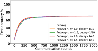
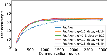
We evaluate the performance of different algorithms with a wide range of hyper-parameters, summarized in Table 5. In particular, following Anstreicher and Wolsey, (2009) we tried sublinear $O(1/t)$ and exponential decay $O({\beta }^t)$ learning rates $\mathrm{\eta }$ on the server, and a fixed local learning rate $\eta$ for client updates. Eventually we settled on decaying ${\mathrm{\eta }}_t$ by a factor of $\beta$ every $100$ steps: ${\mathrm{\eta }}_t={\beta }^{[\frac{t}{100}]}$, where $\beta ={\text{decay}}^{100/T}$ and $T$ is the total number of communication rounds (with e.g. decay = $1/10$). We note that Reddi et al., (2020) also found exponential decay to be most effective in their experiments. We use grid search to choose suitable local learning rates for all algorithms.

Figure 1: Interpolation between FedAvg and FedMGDA on CIFAR-10. $x$-axis is the number of communication rounds. From left to right: (a) and (b) Average user accuracy in non-iid/iid setting resp. (c) and (d) Uniformly averaged training loss in non-iid/iid setting resp. Results are averaged over $5$ runs with different random seeds.

Figure 2: (Left) Test accuracy of SOTA algorithms on Adult dataset with adversarial biases added to the loss of PhD domain; and compared to the baseline of training only on PhD domain. The scales of biases for AFL and q-FedAvg are different because AFL uses averaged loss while q-FedAvg uses (non-averaged) total loss. (Right) Test accuracy of different algorithms on CIFAR-10 in the presence of a malicious user who scales its loss function with a constant factor. All algorithms are run for $500$ rounds on Adult and $1500$ rounds on CIFAR-10. The reported results are averaged across $5$ runs with different random seeds. For detailed hyperparameter setting, see Section B.2.

We evaluate our algorithm FedMGDA+ on several public datasets: CIFAR-10 (Krizhevsky,, 2009), F-MNIST (Xiao et al.,, 2017), Federated EMNIST (Caldas et al.,, 2018), Shakespeare (Li et al., 2020a, ) and Adult (Dua and Graff,, 2017), and compare to existing FL systems including FedAvg (McMahan et al.,, 2017), FedProx (Li et al., 2020a, ), q-FedAvg (Li et al., 2020b, ), and AFL (Mohri et al.,, 2019). In addition, from the discussions in §5, one can envision several potential extensions of existing algorithms to improve their performance. So, we also compare to the following extensions: FedAvg-n which is FedAvg with gradient normalization, and MGDA-Prox which is FedMGDA+ with a proximal regularizer added to each user’s loss function. We distinguish between FedMGDA+ and FedMGDA which is a vanilla extension of MGDA to FL.

We point out that FL algorithms are to be deployed on smart devices with moderate computational capabilities. Thus, the models we chose to experiment on are medium-sized (see Tables 2, 3 and 4 for details), with similar complexity to the ones in FedAvg, q-FedAvg and AFL. Due to space limits we only report some representative results in the main paper, and defer the full set of experiments to Appendix B.

6.2 Experimental results

In this subsection we report experimental results about our proposed algorithm FedMGDA+ and compare it with state-of-the-art (SOTA) alternatives under a variety of performance metrics, including accuracy, robustness and fairness. We remind that the accuracy metric is exactly what FedAvg aims to optimize during training, and hence it has some advantage in this metric over other alternative algorithms such as FedMGDA+, AFL, and q-FedAvg, which all aim to bring some fairness among users, perhaps at some occasional, and hopefully small, loss of accuracy.

6.2.1 Recovering FedAvg

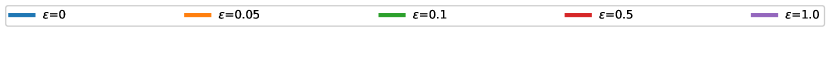
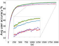
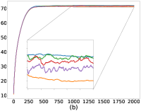
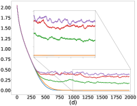
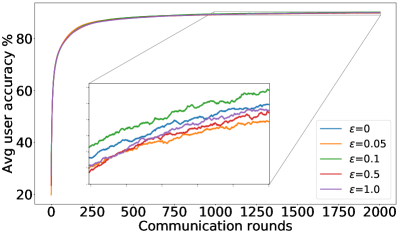
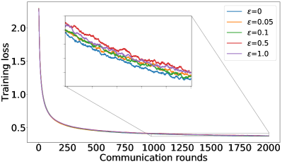
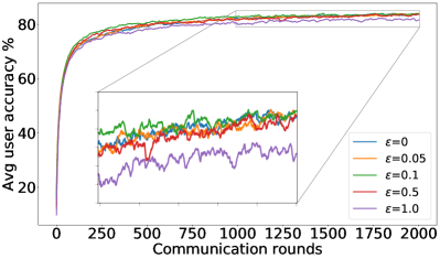
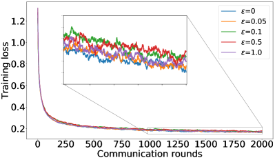
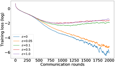
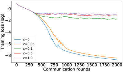
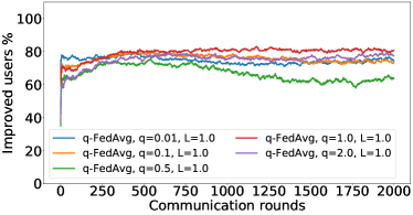
As mentioned in §5, we can control the balance between the user average performance and fairness by tuning the $ϵ$-constraint in Equation 25. Setting $ϵ=0$ recovers FedAvg while setting $ϵ=1$ recovers FedMGDA. To verify this empirically, we run (25) with different $ϵ$, and report results on CIFAR-10 in Figure 1 for both iid and non-iid distributions of data (for results on F-MNIST, see Section B.1). These results confirm that changing $ϵ$ from $0$ to $1$ yields an interpolation between FedAvg and FedMGDA, as expected. Since FedAvg essentially optimizes the (uniformly) averaged training loss, it naturally performs the best under this metric (Figure 1 (c) and (d)). Nevertheless, it is interesting to note that some intermediate $ϵ$ values actually lead to better user accuracy than FedAvg in the non-iid setting (Figure 1 (a)).

Figure 3: Distribution of the user test accuracy on CIFAR-10: (Left) the algorithms are run for $2000$ communication rounds and $b=10$. The hyperparameters are: $\mu =0.01$ for FedProx; $\mathrm{\eta }=1.5$ and $\text{decay}=1/10$ for FedMGDA+ and FedAvg; $\mathrm{\eta }=1.0$ and $\text{decay}=1/10$ for MGDA-Prox; $q=0.5$ and $L=1.0$ for q-FedAvg. (Right) the algorithms are run for $3000$ communication rounds and $b=400$. The hyperparameters are: $\mu =0.5$ for FedProx; $\mathrm{\eta }=1.0$ and $\text{decay}=1/40$ for FedMGDA+, MGDA-Prox, and FedAvg; $q=0.1$ and $L=0.1$ for q-FedAvg. The reported statistics are averaged across $4$ runs with different random seeds.

Figure 4: The percentage of improved users in terms of training loss vs communication rounds on the CIFAR-10 dataset. Two representative cases are shown: (Left) the local batch size $b=10$, and (Right) the local batch size $b=400$. The results are averaged across $4$ runs with different random seeds.

6.2.2 Robustness

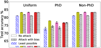
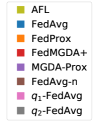
We discussed earlier in §5 that the gradient normalization and MGDA’s built-in robustness allow FedMGDA+ to combat against certain adversarial attacks in practical FL deployment. We now empirically evaluate the robustness of FedMGDA+ against these attacks. We run various FL algorithms in the presence of a single malicious user who aims to manipulate the system by inflating its loss. We consider an adversarial setting where the attacker participates in each communication round and inflates its loss function by (i) adding a bias to it, or (ii) multiplying it by a scaling factor, termed the bias and scaling attack, respectively. In the first experiment, we simulate a bias attack on the Adult dataset by adding a constant bias to the underrepresented user, i.e. the PhD domain, since it’s more natural to expect an attacker to be consisted of a small number of users. In this setup, the worst performance we can get is bounded by training the model using PhD data only. Results under the bias attack are presented in Figure 2 (Left); also see Section B.2 for more results. We observe that AFL and q-FedAvg perform slightly better than FedMGDA+ without the attack; however, their performances deteriorate to a level close to the worst case scenario under the attack. In contrast, FedMGDA+ is not affected by the attack with any bias, which empirically supports our claim in §5. Note that we did not include FedAvg in this comparison since from its definition it is clear that FedAvg, like FedMGDA+, is not affected by the bias attack. Figure 2 (Right) shows the results of different algorithms on CIFAR-10 with and without an adversarial scaling. As mentioned earlier, q-FedAvg with gradient normalization is highly unstable particularly under the scaling attack, so we did not include its result here. From Figure 2 (Right) it is immediate to see that (i) the scaling attack affects all algorithms that do not employ gradient normalization; (ii) q-FedAvg is the most affected under this attack; (iii) surprisingly, FedMGDA+ and, to a lesser extent, MGDA-Prox actually converge to slightly better Pareto solutions, compared to their own results under no scaling attack. The above results empirically verify the robustness of FedMGDA+ under perhaps the most common bias and scaling attacks.

6.2.3 Fairness

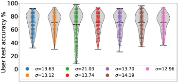
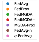
Lastly, we compare FedMGDA+ with existing FL algorithms using different notions of fairness on CIFAR-10. For the first experiment, we adopt the same fairness metric as (Li et al., 2020b, ), and measure fairness by calculating the variance of users’ test error. We run each algorithm with different hyperparameters, and among the results, we pick the best ones in terms of average accuracy to be shown in Figure 3; full table of results can be found in Section B.3. From this figure, we observe that (i) FedMGDA+ achieves the best average accuracy while its standard deviation is comparable with that of q-FedAvg; (ii) FedMGDA+ significantly outperforms FedMGDA, which clearly justifies our proposed modifications in Algorithm 1 to the vanilla MGDA; and (iii) FedMGDA+ outperforms FedAvg-n, which uses the same normalization step as FedMGDA+, in terms of average accuracy and standard deviation. These observations confirm the effectiveness of FedMGDA+ in inducing fairness. We perform the same experiment on the Federated EMNIST dataset, and observed similar results, which can be found in Table 6 and Section B.4.

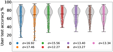
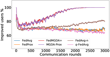
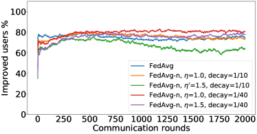
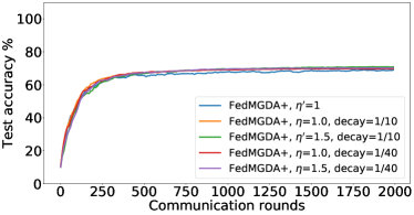
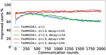
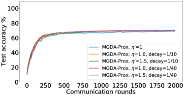
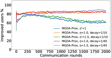
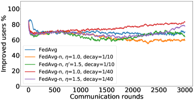
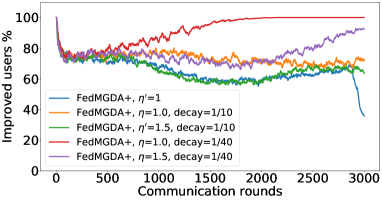
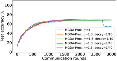
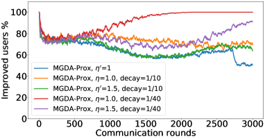
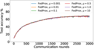
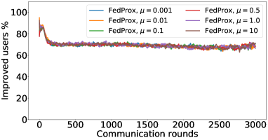
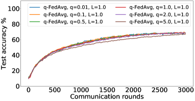
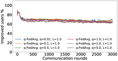
In the next experiment, we show that FedMGDA+ not only yields a fair final solution but also maintains fairness during the entire training process in the sense that, in each round, it refrains from sacrificing the performance of any participating user for the sake of improving the overall performance. To the best of our knowledge, “fairness during training” has not been investigated before, in spite of having great practical implications—it encourages user participation. To examine this fairness, we run several experiments on CIFAR-10 and measure the percentage of improved participants in each communication round. Specifically, we measure the training loss before and after each round for all participating users, and report the percentage of those improved or stay unchanged. Figure 4 shows the percentage of improved participating users in each communication round in terms of training loss for two representative cases; see Section B.5 for full results with different hyperparameters.

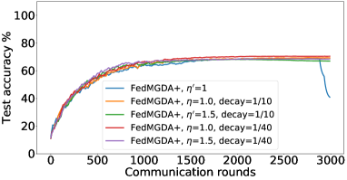
We can see that FedMGDA+ consistently outperforms other algorithms in terms of percentage of improved users, which means that by using FedMGDA+, fewer users’ performances get worse after each participation. Furthermore, we notice from Figure 4 (Left) that, with local batch size $b=10$, the percentage of improved users is less than $100$%, which can be explained as follows: for small batch sizes (i.e., where $𝒟$ represents a local dataset), the received updates from users are not the true gradients of users’ losses given the global model (i.e., ${𝐠}_i\ne \nabla f_i(𝐰)$); they are noisy estimates of the true gradients. Consequently, the common descent direction calculated by MGDA is noisy and may not always work for all participating users. To remove the effect of this noise, we set $b=|𝒟|$ which allows us to recover the true gradients from the users. The results are presented in Figure 4 (Right), which confirms that, when step size decays (less overshooting), the percentage of improved users for FedMGDA+ reaches towards $100$% during training, as is expected.

Table 6: Test accuracy of users on federated EMNIST with full batch, $10$ users per rounds, local learning rate $\eta =0.1$, total communication rounds $1500$. The reported statistics are averaged across $4$ runs with different random seeds.

Algorithm	Average (%)	Std. (%)
FedMGDA	$85.73\pm 0.05$	$14.79\pm 0.12$
FedMGDA+	$87.60\pm 0.20$	$13.68\pm 0.19$
MGDA-Prox	$87.59\pm 0.19$	$13.75\pm 0.18$
FedAvg	$84.97\pm 0.44$	$15.25\pm 0.36$
FedAvg-n	$87.57\pm 0.09$	$13.74\pm 0.11$
FedProx	$84.97\pm 0.45$	$15.26\pm 0.35$
q-FedAvg	$84.97\pm 0.44$	$15.25\pm 0.37$

7 Conclusion

We have proposed a novel algorithm FedMGDA+ for federated learning. FedMGDA+ is based on multi-objective optimization and aims to converge to Pareto stationary solutions. FedMGDA+ is simple to implement, has fewer hyperparameters to tune, and complements existing FL systems nicely. Most importantly, FedMGDA+ is robust against additive and multiplicative adversarial manipulations and ensures fairness among all participating users. We established preliminary convergence guarantees for FedMGDA+, pointed out its connections to recent FL algorithms, and conducted extensive experiments to verify its effectiveness. In the future we plan to formally quantify the tradeoff induced by multiple local updates and to establish some privacy guarantee for FedMGDA+.

Appendix A Proofs

Theorem 1a (full version).

Suppose each user function $f_i$ is $L$-Lipschitz smooth (i.e., ${\nabla }^2{f}_i⪯L𝐈$) and $M$-Lipschitz continuous. Then, with step size ${\mathrm{\eta }}_t\in (0,\frac{1}{2L}]$ we have

$\underset{t=0,\mathrm{\dots },T}{\min }𝐄[\Vert J_{𝐟}({𝐰}_t){𝝀}_t\Vert ]\le {\displaystyle \frac{2[𝐟({𝐰}_0)-\mathrm{𝐄𝐟}({𝐰}_{T+1})+{\sum }_{t=0}^T{\mathrm{\eta }}_t(M{\sigma }_t+L{\mathrm{\eta }}_t{\sigma }_t^2)]}{{\sum }_{t=0}^T{\mathrm{\eta }}_t}},$ (31)

where ${\sigma }_t^2:=𝐄{\Vert J_{𝐟}({𝐰}_t){𝛌}_t-{\widehat{J}}_{𝐟}({𝐰}_t){\widehat{𝛌}}_t\Vert }^2$ is the variance of the stochastic common direction. Moreover, if some user function $f_i$ is bounded from below, and it is possible to choose ${\mathrm{\eta }}_t$ so that , then the left-hand side in (31) converges to 0.

Proof.

Let ${𝝃}_t:=J_{𝐟}({𝐰}_t){𝝀}_t-{\widehat{J}}_{𝐟}({𝐰}_t){\widehat{𝝀}}_t$, where ${\widehat{J}}_{𝐟}({𝐰}_t):=[\widehat{\nabla }{f}_1({𝐰}_t),\mathrm{\dots },\widehat{\nabla }{f}_m({𝐰}_t)]$ is the concatenation of stochastic gradients at each user, and

${𝝀}_t=\underset{𝝀\in \mathrm{\Delta }}{\text{argmin}}\Vert J_{𝐟}({𝐰}_t)𝝀\Vert ,{\widehat{𝝀}}_t=\underset{\widehat{𝝀}\in \mathrm{\Delta }}{\text{argmin}}\Vert {\widehat{J}}_{𝐟}({𝐰}_t)\widehat{𝝀}\Vert ,$ (32)

where for the latter we also constrain ${\widehat{\lambda }}_i=0$ if the $i$-th user is not participating in round $t$. Then, applying the quadratic bound and the update rule (we remind that comparison between vector and scalar should be understood as component-wise):

$𝐟({𝐰}_{t+1})$ $\le 𝐟({𝐰}_t)-{\mathrm{\eta }}_t{J}_{𝐟}^{\top }({𝐰}_t){\widehat{J}}_{𝐟}({𝐰}_t){\widehat{𝝀}}_t+{\displaystyle \frac{L{\mathrm{\eta }}_t^2}{2}}{\Vert {\widehat{J}}_{𝐟}({𝐰}_t){\widehat{𝝀}}_t\Vert }^2$ (33)

$\le 𝐟({𝐰}_t)-{\mathrm{\eta }}_t{J}_{𝐟}^{\top }({𝐰}_t)J_{𝐟}({𝐰}_t){𝝀}_t+L{\mathrm{\eta }}_t^2{\Vert J_{𝐟}({𝐰}_t){𝝀}_t\Vert }^2+{\mathrm{\eta }}_t{J}_{𝐟}^{\top }({𝐰}_t){𝝃}_t+L{\mathrm{\eta }}_t^2{\Vert {𝝃}_t\Vert }^2$ (34)

$\le 𝐟({𝐰}_t)-{\mathrm{\eta }}_t(1-L{\mathrm{\eta }}_t){\Vert J_{𝐟}({𝐰}_t){𝝀}_t\Vert }^2+{\mathrm{\eta }}_{t}M\Vert {𝝃}_t\Vert +L{\mathrm{\eta }}_t^2{\Vert {𝝃}_t\Vert }^2,$ (35)

where we used the Lipschitz continuity $\Vert \nabla f_i(𝐰)\Vert \le M$ and the first-order optimality condition of ${𝝀}_t$ so that

$\forall 𝝀\in \mathrm{\Delta },⟨𝝀,J_{𝐟}^{\top }({𝐰}_t)J_{𝐟}({𝐰}_t){𝝀}_t⟩\ge ⟨{𝝀}_t,J_{𝐟}^{\top }({𝐰}_t)J_{𝐟}({𝐰}_t){𝝀}_t⟩.$ (36)

Letting ${\mathrm{\eta }}_t\le \frac{1}{2L}$, taking expectations and rearranging we obtain

$\underset{t=0,\mathrm{\dots },T}{\min }𝐄[\Vert J_{𝐟}({𝐰}_t){𝝀}_t\Vert ]\le {\displaystyle \frac{2[𝐟({𝐰}_0)-\mathrm{𝐄𝐟}({𝐰}_{T+1})+{\sum }_{t=0}^T{\mathrm{\eta }}_t(M{\sigma }_t+L{\mathrm{\eta }}_t{\sigma }_t^2)]}{{\sum }_{t=0}^T{\mathrm{\eta }}_t}},$ (37)

where ${\sigma }_t^2:=𝐄{\Vert {𝝃}_t\Vert }^2$. ∎

Theorem 1b (full version).

Suppose each user function $f_i$ is $L$-Lipschitz smooth (i.e., ${\nabla }^2{f}_i⪯L𝐈$) and $M$-Lipschitz continuous. Then, for any number of local updates $k$, with global learning rate ${\mathrm{\eta }}_t\in (0,\frac{1}{2L}]$, deterministic gradient update and local learning rate ${\eta }_t^l$, we have

$\underset{t=0,\mathrm{\dots },T}{\min }\Vert J_{𝐟}({𝐰}_t){𝝀}_t\Vert \le {\displaystyle \frac{2\left[𝐟({𝐰}_0)-𝐟({𝐰}_{T+1})+M^2{\mathrm{\eta }}_t{\sum }_{t=0}^T\left(\left({\epsilon }_t\sqrt{m}+{\eta }_t^l(k-1)\right)+L{\mathrm{\eta }}_t{\left({\epsilon }_t\sqrt{m}+{\eta }_t^l(k-1)\right)}^2\right)\right]}{{\sum }_{t=0}^T{\mathrm{\eta }}_t}},$ (38)

where ${\epsilon }_t:=\Vert {𝛌}_t-{\widetilde{𝛌}}_t\Vert$ is the deviation between the exact and approximate (dual) weightings. Moreover, if some user function $f_i$ is bounded from below, then the left-hand side in (38) converges to 0 as long as ${\epsilon }_t\to 0$ , ${\eta }_t^l\to 0$ and ${\mathrm{\eta }}_t\to 0$ with ${\sum }_t{\mathrm{\eta }}_t=\mathrm{\infty }$.

Proof.

Let

${𝝀}_t=\underset{𝝀\in \mathrm{\Delta }}{\text{argmin}}\Vert J_{𝐟}({𝐰}_t)𝝀\Vert ,{\widetilde{𝝀}}_t=\underset{𝝀\in \mathrm{\Delta }}{\text{argmin}}\Vert {\tilde{J}}_{𝐟}({𝐰}_t)𝝀\Vert ,$ (39)

and ${\delta }_t:=J_{𝐟}({𝐰}_t){𝝀}_t-{\tilde{J}}_{𝐟}({𝐰}_t){\widetilde{𝝀}}_t$, where ${\tilde{J}}_{𝐟}({𝐰}_t):=[\tilde{\nabla }{f}_1({𝐰}_t),\mathrm{\dots },\tilde{\nabla }{f}_m({𝐰}_t)]$ is the concatenation of accumulated updates $\tilde{\nabla }{f}_i({𝐰}_t)$ at each user. Formally, $\tilde{\nabla }{f}_i({𝐰}_t):={𝐰}_t-{𝐰}_t^k$, which denotes the difference between the initial ${𝐰}_t$ and the final ${𝐰}_t^k$ after $k$ local updates, for user $i$. (Note that we have abused the notation ${𝐰}_t$ and ${𝐰}_t^k$ a bit for simplicity here, as they do not distinguish user $i$. This is not a big problem since the context is clear.)

Let ${𝐰}_t^1:={𝐰}_t-\nabla f_i({𝐰}_t)$ and ${𝐰}_t^{j+1}:={𝐰}_t^j-{\eta }_t^l\nabla f_i({𝐰}_t^j),j=1,\mathrm{\dots },k-1$ be the local optimization steps.

Then,

$\tilde{\nabla }{f}_i({𝐰}_t)$ $={𝐰}_t-{𝐰}_t^k$ (40)

$=({𝐰}_t-{𝐰}_t^1)+({𝐰}_t^1-{𝐰}_t^2)+\mathrm{\dots }+({𝐰}_t^{k-1}-{𝐰}_t^k)$ (41)

$=\nabla f_i({𝐰}_t)+{\eta }_t^l\nabla f_i({𝐰}_t^1)+\mathrm{\dots }+{\eta }_t^l\nabla f_i({𝐰}_t^{k-1}),$ (42)

Thus, the difference between $\tilde{\nabla }{f}_i({𝐰}_t)$ and gradient $\nabla f_i({𝐰}_t)$ is bounded by:

$\Vert \tilde{\nabla }{f}_i({𝐰}_t)-\nabla f_i({𝐰}_t)\Vert$ $=\Vert {\eta }_t^l{\displaystyle \sum _{j=1}^{k-1}}\nabla f_i({𝐰}_t^j)\Vert$ (44)

$\le {\eta }_t^l{\displaystyle \sum _{j=1}^{k-1}}\Vert \nabla f_i({𝐰}_t^j)\Vert$ (45)

$\le {\eta }_t^l(k-1)M,$ (46)

Thus,

$\Vert {\delta }_t\Vert$ $=\Vert J_{𝐟}({𝐰}_t){𝝀}_t-{\tilde{J}}_{𝐟}({𝐰}_t){\widetilde{𝝀}}_t\Vert$ (47)

$\le \Vert J_{𝐟}({𝐰}_t){𝝀}_t-J_{𝐟}({𝐰}_t){\widetilde{𝝀}}_t\Vert +\Vert J_{𝐟}({𝐰}_t){\widetilde{𝝀}}_t-{\tilde{J}}_{𝐟}({𝐰}_t){\widetilde{𝝀}}_t\Vert$ (48)

$\le {\epsilon }_t\sqrt{m}M+{\eta }_t^l(k-1)M,$ (49)

the last step comes from matrix norm inequality on the first term, and triangular inequality on the second term. Note that $\Vert {\delta }_t\Vert$ vanishes when ${\epsilon }_t\to 0$ and ${\eta }_t^l\to 0$.

Then, applying the quadratic upper bound, we have

$𝐟({𝐰}_{t+1})$ $\le 𝐟({𝐰}_t)-{\mathrm{\eta }}_t{J}_{𝐟}^{\top }({𝐰}_t){\tilde{J}}_{𝐟}({𝐰}_t){\widetilde{𝝀}}_t+{\displaystyle \frac{L{\mathrm{\eta }}_t^2}{2}}{\Vert {\tilde{J}}_{𝐟}({𝐰}_t){\widetilde{𝝀}}_t\Vert }^2$ (50)

$=𝐟({𝐰}_t)-{\mathrm{\eta }}_t{J}_{𝐟}^{\top }({𝐰}_t)J_{𝐟}({𝐰}_t){𝝀}_t+L{\mathrm{\eta }}_t^2{\Vert J_{𝐟}({𝐰}_t){𝝀}_t\Vert }^2+{\mathrm{\eta }}_t{J}_{𝐟}^{\top }({𝐰}_t){\delta }_t+L{\mathrm{\eta }}_t^2{\Vert {\delta }_t\Vert }^2$ (51)

$\le 𝐟({𝐰}_t)-{\mathrm{\eta }}_t(1-L{\mathrm{\eta }}_t){\Vert J_{𝐟}({𝐰}_t){𝝀}_t\Vert }^2+{\mathrm{\eta }}_{t}M\Vert {\delta }_t\Vert +L{\mathrm{\eta }}_t^2{\Vert {\delta }_t\Vert }^2,$ (52)

Letting ${\mathrm{\eta }}_t\le \frac{1}{2L}$, telescoping and rearranging we obtain

$\underset{t=0,\mathrm{\dots },T}{\min }\Vert J_{𝐟}({𝐰}_t){𝝀}_t\Vert \le {\displaystyle \frac{2[𝐟({𝐰}_0)-𝐟({𝐰}_{T+1})+{\sum }_{t=0}^T{\mathrm{\eta }}_t(M\Vert {\delta }_t\Vert +L{\mathrm{\eta }}_t{\Vert {\delta }_t\Vert }^2)]}{{\sum }_{t=0}^T{\mathrm{\eta }}_t}},$ (53)

substitute $\Vert {\delta }_t\Vert$ with (49), and we get (38).

Finally, if ${\epsilon }_t\to 0$ and ${\eta }_t^l\to 0$, then ${\delta }_t\to 0$ and hence the right-hand side in (38) $\to 0$ when $T\to \mathrm{\infty }$, in which case the left-hand side ${\min }_{t=0,\mathrm{\dots },T}\Vert J_{𝐟}({𝐰}_t){𝝀}_t\Vert$ converges to $0$ as well. ∎

Theorem 2 (full version).

Suppose each user function $f_i$ is $\sigma$-strongly convex (i.e. ${\nabla }^2{f}_i⪰\sigma 𝐈$) and $M$-Lipschitz continuous. Suppose at each round $t$ FedMGDA includes some function $f_{v_t}$ such that

$f_{v_t}({𝐰}_t)-f_{v_t}({𝐰}_t^{\ast })\ge \frac{{\mathrm{\ell }}_t}{2}{\Vert {𝐰}_t-{𝐰}_t^{\ast }\Vert }^2,$ (54)

where ${𝐰}_t^{\ast }$ is the projection of ${𝐰}_t$ to the Pareto stationary set $W^{\ast }$ of (11). Assume $𝐄[{\lambda }_{v_t}{\mathrm{\ell }}_t+{\sigma }_t|{𝐰}_t]\ge c>0$, then

$𝐄[{\Vert {𝐰}_{t+1}-{𝐰}_{t+1}^{\ast }\Vert }^2]\le {\pi }_t(1-c{\mathrm{\eta }}_0)𝐄[{\Vert {𝐰}_0-{𝐰}_0^{\ast }\Vert }^2]+{\displaystyle \sum _{s=0}^t}{\displaystyle \frac{{\pi }_t}{{\pi }_s}}{\mathrm{\eta }}_s^2{M}^2,$ (55)

where ${\pi }_t={\prod }_{s=1}^t{\mathrm{\eta }}_s$ and ${\pi }_0=1$. In particular,

• if , then $𝐄[{\Vert {𝐰}_t-{𝐰}_t^{\ast }\Vert }^2]\to 0$ and ${𝐰}_t$ converges to the Pareto stationarity set $W^{\ast }$ almost surely;

• with the choice ${\mathrm{\eta }}_t=\frac{2}{c(t+2)}$ we have

  $𝐄[{\Vert {𝐰}_t-{𝐰}_t^{\ast }\Vert }^2]\le {\displaystyle \frac{4M^2}{c^2(t+3)}}.$ (56)

Proof.

For each user $i$, let us define the function

${\widehat{f}}_i(𝐰,I):=I_i{f}_i(𝐰),$ (57)

where the random variable $I\in {\{0,1\}}^m$ indicates which user participates at a particular round. Clearly, we have $𝐄{\widehat{f}}_i(𝐰,I)=f_i(𝐰)𝐄I_i$. Therefore, our multi-objective minimization problem is equivalent as:

$\underset{𝐰}{\min }\{𝐄{\widehat{f}}_1(𝐰,I),\mathrm{\dots },𝐄{\widehat{f}}_m(𝐰,I)\},$ (58)

since positive scaling does not change Pareto stationarity. (If one prefers, we can also normalize the stochastic functions ${\widehat{f}}_i(𝐰,I)$ so that the unbiasedness property $𝐄{\widehat{f}}_i(𝐰,I)=f_i(𝐰)$ holds.)

We now proceed as in Mercier et al., (2018) and provide a slightly sharper analysis. Let us denote ${𝐰}_t^{\ast }$ the projection of ${𝐰}_t$ to the Pareto-stationary set $W^{\ast }$ of (58), i.e.,

${𝐰}_t^{\ast }=\underset{𝐰\in W^{\ast }}{\text{argmin}}\Vert {𝐰}_t-𝐰\Vert .$ (59)

Then,

${\Vert {𝐰}_{t+1}-{𝐰}_{t+1}^{\ast }\Vert }^2$ $\le {\Vert {𝐰}_{t+1}-{𝐰}_t^{\ast }\Vert }^2$ (60)

$={\Vert {𝐰}_t-{\mathrm{\eta }}_t{𝐝}_t-{𝐰}_t^{\ast }\Vert }^2$ (61)

$={\Vert {𝐰}_t-{𝐰}_t^{\ast }\Vert }^2-2{\mathrm{\eta }}_t⟨{𝐰}_t-{𝐰}_t^{\ast },{𝐝}_t⟩+{\mathrm{\eta }}_t^2{\Vert {𝐝}_t\Vert }^2.$ (62)

To bound the middle term, we have from our assumption:

$\exists v_t,{\widehat{f}}_{v_t}({𝐰}_t,I_t)-{\widehat{f}}_{v_t}({𝐰}_t^{\ast },I_t)$ $\ge \frac{{\mathrm{\ell }}_t}{2}{\Vert {𝐰}_t-{𝐰}_t^{\ast }\Vert }^2,$ (63)

$\forall i,{\widehat{f}}_i({𝐰}_t,I_t)-{\widehat{f}}_i({𝐰}_t^{\ast },I_t)$ $\ge 0,$ (64)

where the second inequality follows from the definition of ${𝐰}_t^{\ast }$. Therefore,

$⟨{𝐰}_t-{𝐰}_t^{\ast },{𝐝}_t⟩$ $=⟨{𝐰}_t-{𝐰}_t^{\ast },{\displaystyle \sum _{i:I_i=1}}{\lambda }_i\nabla f_i({𝐰}_t)⟩$ (65)

$\ge {\displaystyle \sum _{i:I_i=1}}{\lambda }_i\left(f_i({𝐰}_t)-f_i({𝐰}_t^{\ast })\right)+\frac{{\sigma }_t}{2}{\Vert {𝐰}_t-{𝐰}_t^{\ast }\Vert }^2$ (66)

$={\displaystyle \sum _i}{\lambda }_i\left({\widehat{f}}_i({𝐰}_t,I_t)-{\widehat{f}}_i({𝐰}_t^{\ast },I_t)\right)+\frac{{\sigma }_t}{2}{\Vert {𝐰}_t-{𝐰}_t^{\ast }\Vert }^2$ (67)

$\ge \frac{{\lambda }_{v_t}{\mathrm{\ell }}_t+{\sigma }_t}{2}{\Vert {𝐰}_t-{𝐰}_t^{\ast }\Vert }^2.$ (68)

Continuing from (62) and taking conditional expectation:

$𝐄[{\Vert {𝐰}_{t+1}-{𝐰}_{t+1}^{\ast }\Vert }^2|{𝐰}_t]$ $\le (1-c_t{\mathrm{\eta }}_t){\Vert {𝐰}_t-{𝐰}_t^{\ast }\Vert }^2+{\mathrm{\eta }}_t^2{M}^2,$ (69)

where $c_t:=𝐄[{\lambda }_{v_t}{\mathrm{\ell }}_t+{\sigma }_t|{𝐰}_t]\ge c>0$. Taking expectation we obtain the familiar recursion:

$𝐄[{\Vert {𝐰}_{t+1}-{𝐰}_{t+1}^{\ast }\Vert }^2]$ $\le (1-c{\mathrm{\eta }}_t)𝐄[{\Vert {𝐰}_t-{𝐰}_t^{\ast }\Vert }^2]+{\mathrm{\eta }}_t^2{M}^2,$ (70)

from which we derive

$𝐄[{\Vert {𝐰}_{t+1}-{𝐰}_{t+1}^{\ast }\Vert }^2]$ $\le {\pi }_t(1-c{\mathrm{\eta }}_0)𝐄[{\Vert {𝐰}_0-{𝐰}_0^{\ast }\Vert }^2]+{\displaystyle \sum _{s=0}^t}\frac{{\pi }_t}{{\pi }_s}{\mathrm{\eta }}_s^2{M}^2,$ (71)

where ${\pi }_t={\prod }_{s=1}^t(1-c{\mathrm{\eta }}_s)$ and ${\pi }_0=1$. Since ${\pi }_t\to 0\iff {\sum }_t{\mathrm{\eta }}_t=\mathrm{\infty }$, we know

$𝐄[{\Vert {𝐰}_{t+1}-{𝐰}_{t+1}^{\ast }\Vert }^2]\to 0$ (72)

if ${\sum }_t{\mathrm{\eta }}_t=\mathrm{\infty }$ and .

Setting ${\mathrm{\eta }}_t=\frac{2}{c(t+2)}$ we obtain ${\pi }_t=\frac{2}{(t+2)(t+1)}$ and by induction

${\displaystyle \sum _{s=0}^t}{\displaystyle \frac{{\pi }_t}{{\pi }_s}}{\mathrm{\eta }}_s^2={\displaystyle \frac{4}{c^2(t+2)(t+1)}}{\displaystyle \sum _{s=0}^t}{\displaystyle \frac{s+1}{s+2}}\le {\displaystyle \frac{4}{c^2(t+4)}},$ (73)

whence

$𝐄[{\Vert {𝐰}_{t+1}-{𝐰}_{t+1}^{\ast }\Vert }^2]\le {\displaystyle \frac{4M^2}{c^2(t+4)}}.$ (74)

Using a standard supermartingale argument we can also prove that

${𝐰}_t-{𝐰}_t^{\ast }\to 0\text{almost surely}.$ (75)

The proof is well-known in stochastic optimization hence omitted (or see Mercier et al., (2018, Theorem 5) for details). ∎

Appendix B Full experimental results

In this section we provide additional results that are deferred from the main paper.

B.1 Recovering FedAvg full results: results on Fashion-MNIST and CIFAR-10

Complementary to the results shown in Figure 1, Figure 5 and Figure 6 summarize similar results on the F-MNIST dataset, while Figure 7 depicts the training losses on CIFAR-10 dataset in log-scale.

Figure 5: Interpolation between FedAvg and FedMGDA (F-MNIST, iid setting). (Left) Average user accuracy. (Right) Uniformly averaged training loss. Results are averaged over $5$ runs with different random seeds.

Figure 6: Interpolation between FedAvg and FedMGDA (F-MNIST, non-iid setting). (Left) Average user accuracy. (Right) Uniformly averaged training loss. Results are averaged over $5$ runs with different random seeds.

Figure 7: Interpolation between FedAvg and FedMGDA (CIFAR-10). Both figures plot the uniformly averaged training loss in log-scale. (Left) non-iid setting. (Right) iid setting. Results are averaged over $5$ runs with different random seeds.

B.2 Robustness full results: bias attack on Adult dataset

Table 7 shows the full results of the experiment presented in Figure 2 (Left).

Table 7: Test accuracy of SOTA algorithms on Adult dataset with various scales of adversarial bias added to the domain loss of PhD; and compared to the baseline of training only on the PhD domain. The scale of bias for AFL is different from q-FedAvg since AFL uses averaged loss while q-FedAvg uses (non-averaged) total loss. The algorithms are run for $500$ rounds, and the reported results are averaged across $5$ runs with different random seeds.

Name	Bias	Uniform	PhD	Non-PhD
AFL	$0$	$83.26\pm 0.01$	$77.90\pm 0.00$	$83.32\pm 0.01$
AFL	$0.01$	$83.28\pm 0.03$	$76.58\pm 0.27$	$83.36\pm 0.03$
AFL	$0.1$	$82.30\pm 0.04$	$74.59\pm 0.00$	$82.39\pm 0.04$
AFL	$1$	$81.86\pm 0.05$	$74.25\pm 0.57$	$81.94\pm 0.05$
q-FedAvg, $q=5$	$0$	$83.26\pm 0.18$	$76.80\pm 0.61$	$83.33\pm 0.19$
q-FedAvg, $q=5$	$1000$	$83.34\pm 0.04$	$76.57\pm 0.44$	$83.41\pm 0.04$
q-FedAvg, $q=5$	$5000$	$81.19\pm 0.03$	$74.14\pm 0.41$	$81.27\pm 0.03$
q-FedAvg, $q=5$	$10000$	$81.07\pm 0.03$	$73.48\pm 0.78$	$81.16\pm 0.02$
q-FedAvg, $q=2$	$0$	$83.30\pm 0.09$	$76.46\pm 0.56$	$83.38\pm 0.09$
q-FedAvg, $q=2$	$1000$	$83.33\pm 0.04$	$76.24\pm 0.00$	$83.41\pm 0.04$
q-FedAvg, $q=2$	$5000$	$83.11\pm 0.03$	$75.69\pm 0.00$	$83.20\pm 0.03$
q-FedAvg, $q=2$	$10000$	$82.50\pm 0.07$	$75.69\pm 0.00$	$82.58\pm 0.07$
q-FedAvg, $q=0.1$	$0$	$83.44\pm 0.06$	$76.46\pm 0.56$	$83.52\pm 0.07$
q-FedAvg, $q=0.1$	$1000$	$83.34\pm 0.03$	$76.35\pm 0.41$	$83.42\pm 0.02$
q-FedAvg, $q=0.1$	$5000$	$83.35\pm 0.03$	$76.57\pm 0.66$	$83.42\pm 0.03$
q-FedAvg, $q=0.1$	$10000$	$83.36\pm 0.05$	$76.80\pm 0.49$	$83.43\pm 0.05$
FedMGDA+	Arbitrary	$83.24\pm 0.02$	$76.58\pm 0.27$	$83.32\pm 0.02$
Baseline_PhD		$81.05\pm 0.05$	$72.82\pm 0.95$	$81.14\pm 0.05$

The hyper-parameter setting for Figure 2. Left: step sizes ${\gamma }_{\lambda }=0.5$, ${\gamma }_w=0.01$, and bias$=1$ for AFL; $q=5$, and bias$=10000$ for q-FedAvg; $\mathrm{\eta }=1$, decay=$1/3$, and arbitrary bias for FedMGDA+. Right: $\mu =0.01$ for FedProx; $q_1=0.5$ and $q_2=2.0$ for q-FedAvg; $\mathrm{\eta }=1$ and decay=$1/10$ for FedMGDA+ and FedAvg-n. The simulations are run with $20$% user participation ($p=0.2$) in each round which reduces the effectiveness of the adversary since it needs to participate in a bigger pool of users in comparison to our default setting $p=0.1$.

B.3 Fairness full results: first experiment on CIFAR-10

Tables 8, LABEL:, 9, LABEL:, 10, LABEL: and 11 report the full results of the experiment presented in Figure 3 for different batch sizes and fractions of user participation.

Table 8: Test accuracy of users on CIFAR-10 with local batch size $b=10$, fraction of users $p=0.1$, local learning rate $\eta =0.01$, total communication rounds $2000$. The reported statistics are averaged across $4$ runs with different random seeds.

Algorithm			Average (%)	Std. (%)	Worst $5$% (%)	Best $5$% (%)
Name	$\mathrm{\eta }$	decay
FedMGDA			$67.59\pm 0.65$	$21.03\pm 2.40$	$22.95\pm 7.27$	$\mathbf{90.50}\mathbf{\pm }\mathbf{0.87}$
FedMGDA+	$1.0$	$0$	$69.06\pm 1.08$	$14.10\pm 1.61$	$44.38\pm 5.90$	$87.55\pm 0.84$
FedMGDA+	$1.0$	$1/10$	$69.87\pm 0.87$	$14.33\pm 0.61$	$42.42\pm 3.61$	$87.05\pm 0.95$
FedMGDA+	$1.5$	$1/10$	$\mathbf{71.15}\mathbf{\pm }\mathbf{0.62}$	$13.74\pm 0.49$	$44.48\pm 1.64$	$88.53\pm 0.85$
FedMGDA+	$1.0$	$1/40$	$68.68\pm 1.25$	$17.23\pm 1.60$	$34.40\pm 6.23$	$88.07\pm 0.04$
FedMGDA+	$1.5$	$1/40$	$71.05\pm 0.82$	$13.53\pm 0.77$	$\mathbf{46.50}\mathbf{\pm }\mathbf{2.96}$	$88.53\pm 0.85$
Name	$\mathrm{\eta }$	decay
MGDA-Prox	$1.0$	$0$	$66.98\pm 1.52$	$15.46\pm 3.15$	$39.42\pm 10.35$	$87.60\pm 2.18$
MGDA-Prox	$1.0$	$1/10$	$70.39\pm 0.96$	$13.70\pm 1.08$	$46.43\pm 2.17$	$87.50\pm 0.87$
MGDA-Prox	$1.5$	$1/10$	$69.45\pm 0.77$	$14.98\pm 1.61$	$40.42\pm 5.88$	$87.05\pm 1.00$
MGDA-Prox	$1.0$	$1/40$	$69.01\pm 0.51$	$16.24\pm 0.74$	$36.92\pm 4.12$	$88.53\pm 0.85$
MGDA-Prox	$1.5$	$1/40$	$69.53\pm 0.70$	$15.90\pm 1.79$	$36.43\pm 7.42$	$87.53\pm 2.14$
Name	$\mathrm{\eta }$	decay
FedAvg			$70.11\pm 1.27$	$13.63\pm 0.81$	$45.45\pm 2.21$	$88.00\pm 0.00$
FedAvg-n	$1.0$	$0$	$67.69\pm 1.15$	$16.97\pm 2.33$	$37.98\pm 6.61$	$89.55\pm 2.61$
FedAvg-n	$1.0$	$1/10$	$69.66\pm 1.22$	$15.11\pm 1.14$	$40.42\pm 1.71$	$88.55\pm 0.84$
FedAvg-n	$1.5$	$1/10$	$70.62\pm 0.82$	$14.19\pm 0.49$	$43.48\pm 2.17$	$89.03\pm 1.03$
FedAvg-n	$1.0$	$1/40$	$70.31\pm 0.29$	$14.97\pm 0.96$	$42.48\pm 2.56$	$88.55\pm 2.15$
FedAvg-n	$1.5$	$1/40$	$70.47\pm 0.70$	$13.88\pm 0.96$	$44.95\pm 4.07$	$88.03\pm 0.04$
Name	$\mu$
FedProx	$0.01$		$70.77\pm 0.70$	$13.12\pm 0.47$	$46.43\pm 2.95$	$88.50\pm 0.87$
FedProx	$0.1$		$70.69\pm 0.58$	$13.42\pm 0.43$	$45.42\pm 2.14$	$87.55\pm 1.64$
FedProx	$0.5$		$68.89\pm 0.83$	$14.10\pm 1.08$	$43.95\pm 4.52$	$88.00\pm 0.00$
Name	$q$	$L$
q-FedAvg	$0.1$	$0.1$	$70.40\pm 0.41$	$\mathbf{12.43}\mathbf{\pm }\mathbf{0.24}$	$46.48\pm 2.14$	$87.50\pm 0.87$
q-FedAvg	$0.5$	$0.1$	$70.58\pm 0.73$	$13.60\pm 0.47$	$\mathbf{46.50}\mathbf{\pm }\mathbf{2.96}$	$88.05\pm 1.38$
q-FedAvg	$1.0$	$0.1$	$70.27\pm 0.61$	$13.31\pm 0.46$	$45.95\pm 1.38$	$87.55\pm 0.90$
q-FedAvg	$0.1$	$1.0$	$70.95\pm 0.83$	$12.70\pm 0.74$	$46.45\pm 4.07$	$87.00\pm 1.00$
q-FedAvg	$0.5$	$1.0$	$70.98\pm 0.52$	$12.96\pm 0.63$	$45.95\pm 1.45$	$88.00\pm 0.00$
q-FedAvg	$1.0$	$1.0$	$69.98\pm 0.67$	$13.15\pm 1.12$	$45.95\pm 2.49$	$87.53\pm 0.82$

Table 9: Test accuracy of users on CIFAR-10 with local batch size $b=10$, fraction of users $p=0.2$, local learning rate $\eta =0.01$, total communication rounds $2000$. The reported statistics are averaged across $4$ runs with different random seeds.

Algorithm			Average (%)	Std. (%)	Worst $5$% (%)	Best $5$% (%)
Name	$\mathrm{\eta }$	decay
FedMGDA			$66.50\pm 1.77$	$23.22\pm 1.20$	$19.48\pm 4.54$	$\mathbf{91.53}\mathbf{\pm }\mathbf{2.14}$
FedMGDA+	$1.0$	$0$	$66.91\pm 1.15$	$16.28\pm 1.12$	$36.00\pm 6.16$	$88.00\pm 2.00$
FedMGDA+	$1.0$	$1/10$	$\mathbf{70.64}\mathbf{\pm }\mathbf{0.35}$	$16.23\pm 0.84$	$35.95\pm 4.66$	$87.55\pm 0.90$
FedMGDA+	$1.5$	$1/10$	$69.29\pm 0.88$	$13.52\pm 0.69$	$44.45\pm 1.64$	$86.55\pm 0.84$
FedMGDA+	$1.0$	$1/40$	$68.47\pm 0.65$	$18.07\pm 2.84$	$32.95\pm 9.48$	$88.55\pm 2.15$
FedMGDA+	$1.5$	$1/40$	$68.76\pm 0.54$	$17.21\pm 1.28$	$34.43\pm 6.26$	$87.53\pm 0.88$
Name	$\mathrm{\eta }$	decay
MGDA-Prox			$70.06\pm 0.67$	$13.69\pm 0.46$	$42.43\pm 2.99$	$87.03\pm 0.98$
MGDA-Prox	$1.0$	$0$	$68.41\pm 0.88$	$16.30\pm 1.84$	$37.98\pm 3.15$	$89.50\pm 1.66$
MGDA-Prox	$1.0$	$1/10$	$68.19\pm 0.96$	$19.25\pm 2.57$	$28.90\pm 7.02$	$88.55\pm 0.84$
MGDA-Prox	$1.5$	$1/10$	$68.92\pm 0.78$	$14.64\pm 0.59$	$41.42\pm 2.98$	$87.55\pm 1.61$
MGDA-Prox	$1.0$	$1/40$	$68.87\pm 0.60$	$17.47\pm 1.96$	$31.48\pm 7.49$	$89.00\pm 2.24$
MGDA-Prox	$1.5$	$1/40$	$69.29\pm 0.66$	$16.67\pm 1.49$	$35.48\pm 10.31$	$88.03\pm 1.41$
Name	$\mathrm{\eta }$	decay
FedAvg			$69.83\pm 0.69$	$13.17\pm 0.60$	$46.95\pm 1.70$	$86.57\pm 1.64$
FedAvg-n	$1.0$	$0$	$69.05\pm 0.94$	$14.14\pm 1.53$	$39.50\pm 6.22$	$87.50\pm 0.87$
FedAvg-n	$1.0$	$1/10$	$70.52\pm 1.18$	$15.22\pm 1.74$	$39.48\pm 7.90$	$88.03\pm 0.04$
FedAvg-n	$1.5$	$1/10$	$69.27\pm 0.97$	$14.42\pm 0.85$	$43.95\pm 3.76$	$89.00\pm 1.00$
FedAvg-n	$1.0$	$1/40$	$69.34\pm 1.75$	$15.64\pm 2.90$	$38.45\pm 8.50$	$86.53\pm 0.85$
FedAvg-n	$1.5$	$1/40$	$69.87\pm 0.59$	$14.13\pm 0.14$	$43.95\pm 1.42$	$86.57\pm 1.64$
Name	$\mu$
FedProx	$0.01$		$69.74\pm 0.84$	$13.26\pm 0.44$	$47.90\pm 1.45$	$87.50\pm 0.87$
FedProx	$0.1$		$70.06\pm 0.67$	$13.69\pm 0.46$	$42.43\pm 2.99$	$87.03\pm 0.98$
FedProx	$0.5$		$69.64\pm 0.74$	$13.55\pm 0.50$	$44.90\pm 1.67$	$88.00\pm 0.00$
Name	$q$	$L$
q-FedAvg	$0.1$	$0.1$	$70.21\pm 0.71$	$13.23\pm 0.42$	$46.98\pm 0.98$	$87.03\pm 0.98$
q-FedAvg	$0.5$	$0.1$	$70.34\pm 0.71$	$13.05\pm 0.27$	$47.43\pm 1.64$	$88.00\pm 0.00$
q-FedAvg	$1.0$	$0.1$	$70.19\pm 0.79$	$\mathbf{12.79}\mathbf{\pm }\mathbf{0.23}$	$\mathbf{48.42}\mathbf{\pm }\mathbf{0.91}$	$88.00\pm 0.00$
q-FedAvg	$0.1$	$1.0$	$70.18\pm 0.53$	$13.04\pm 0.38$	$47.45\pm 0.84$	$88.05\pm 1.38$
q-FedAvg	$0.5$	$1.0$	$70.30\pm 0.70$	$13.28\pm 1.03$	$45.45\pm 1.71$	$87.55\pm 0.84$
q-FedAvg	$1.0$	$1.0$	$69.39\pm 0.35$	$13.75\pm 0.34$	$43.98\pm 1.41$	$87.08\pm 0.98$

Table 10: Test accuracy of users on CIFAR-10 with local batch size $b=400$, fraction of users $p=0.1$, local learning rate $\eta =0.1$, total communication rounds $3000$. The reported statistics are averaged across $4$ runs with different random seeds.

Algorithm			Average (%)	Std. (%)	Worst $5$% (%)	Best $5$% (%)
Name	$\mathrm{\eta }$	decay
FedMGDA			$68.58\pm 1.99$	$15.56\pm 1.63$	$38.40\pm 6.34$	$87.55\pm 1.61$
FedMGDA+	$1.0$	$0$	$37.62\pm 30.63$	$19.77\pm 5.80$	$21.48\pm 21.58$	$\mathbf{93.03}\mathbf{\pm }\mathbf{6.98}$
FedMGDA+	$1.0$	$1/10$	$68.82\pm 1.56$	$14.66\pm 1.03$	$41.92\pm 3.07$	$87.50\pm 0.87$
FedMGDA+	$1.5$	$1/10$	$67.21\pm 0.89$	$13.76\pm 0.89$	$43.88\pm 2.49$	$85.50\pm 1.66$
FedMGDA+	$1.0$	$1/40$	$\mathbf{70.78}\mathbf{\pm }\mathbf{0.63}$	$\mathbf{12.27}\mathbf{\pm }\mathbf{0.35}$	$\mathbf{47.00}\mathbf{\pm }\mathbf{2.24}$	$87.00\pm 1.00$
FedMGDA+	$1.5$	$1/40$	$67.02\pm 1.04$	$13.44\pm 0.88$	$43.48\pm 1.65$	$85.50\pm 0.87$
Name	$\mathrm{\eta }$	decay
MGDA-Prox	$1.0$	$0$	$52.98\pm 27.14$	$17.18\pm 3.90$	$31.85\pm 18.46$	$91.53\pm 4.96$
MGDA-Prox	$1.0$	$1/10$	$69.10\pm 1.58$	$14.14\pm 0.73$	$43.42\pm 0.83$	$87.50\pm 0.87$
MGDA-Prox	$1.5$	$1/10$	$66.66\pm 0.17$	$14.51\pm 0.37$	$38.00\pm 1.41$	$84.53\pm 0.85$
MGDA-Prox	$1.0$	$1/40$	$69.55\pm 0.52$	$13.40\pm 1.04$	$45.50\pm 3.84$	$86.55\pm 1.61$
MGDA-Prox	$1.5$	$1/40$	$67.77\pm 0.83$	$14.00\pm 0.99$	$41.93\pm 3.78$	$85.53\pm 0.82$
Name	$\mathrm{\eta }$	decay
FedAvg			$66.28\pm 2.04$	$16.92\pm 3.78$	$34.48\pm 11.77$	$87.53\pm 0.82$
FedAvg-n	$1.0$	$0$	$66.11\pm 0.91$	$14.95\pm 0.67$	$36.95\pm 4.32$	$86.03\pm 1.38$
FedAvg-n	$1.0$	$1/10$	$67.76\pm 0.74$	$14.34\pm 0.96$	$40.50\pm 2.18$	$86.50\pm 0.87$
FedAvg-n	$1.5$	$1/10$	$64.04\pm 0.99$	$14.87\pm 1.97$	$35.95\pm 6.12$	$81.55\pm 1.61$
FedAvg-n	$1.0$	$1/40$	$69.50\pm 0.45$	$13.27\pm 0.77$	$44.45\pm 2.92$	$87.03\pm 1.69$
FedAvg-n	$1.5$	$1/40$	$66.54\pm 0.97$	$13.20\pm 0.92$	$42.95\pm 2.21$	$84.07\pm 1.41$
Name	$\mu$
FedProx	$0.01$		$67.43\pm 3.57$	$14.75\pm 1.36$	$40.93\pm 7.87$	$87.05\pm 1.00$
FedProx	$0.1$		$68.35\pm 1.65$	$16.49\pm 2.83$	$36.93\pm 9.97$	$87.05\pm 1.00$
FedProx	$0.5$		$68.89\pm 1.17$	$17.46\pm 3.63$	$29.90\pm 12.64$	$87.05\pm 1.00$
Name	$q$	$L$
q-FedAvg	$0.1$	$0.1$	$70.53\pm 0.73$	$13.34\pm 0.39$	$44.95\pm 4.15$	$89.00\pm 1.73$
q-FedAvg	$0.5$	$0.1$	$67.78\pm 1.81$	$17.56\pm 1.99$	$31.48\pm 10.12$	$90.57\pm 2.21$
q-FedAvg	$1.0$	$0.1$	$66.86\pm 3.02$	$18.56\pm 3.80$	$28.93\pm 11.67$	$87.07\pm 1.69$
q-FedAvg	$0.1$	$1.0$	$64.73\pm 7.39$	$16.01\pm 2.83$	$33.45\pm 10.46$	$84.05\pm 4.71$
q-FedAvg	$0.5$	$1.0$	$68.47\pm 1.74$	$15.33\pm 1.24$	$37.92\pm 4.51$	$87.05\pm 1.00$
q-FedAvg	$1.0$	$1.0$	$69.60\pm 0.98$	$14.19\pm 0.15$	$41.95\pm 5.14$	$88.55\pm 2.95$

Table 11: Test accuracy of users on CIFAR-10 with local batch size $b=400$, fraction of users $p=0.2$, local learning rate $\eta =0.1$, total communication rounds $3000$. The reported statistics are averaged across $4$ runs with different random seeds.

Algorithm			Average (%)	Std. (%)	Worst $5$% (%)	Best $5$% (%)
Name	$\mathrm{\eta }$	decay
FedMGDA			$65.18\pm 5.41$	$16.52\pm 4.70$	$33.95\pm 17.40$	$84.55\pm 1.67$
FedMGDA+	$1.0$	$0$	$6.50\pm 1.66$	$24.40\pm 3.10$	$0.00\pm 0.00$	$75.00\pm 43.30$
FedMGDA+	$1.0$	$1/10$	$70.14\pm 0.72$	$13.53\pm 1.28$	$44.93\pm 2.23$	$87.53\pm 0.88$
FedMGDA+	$1.5$	$1/10$	$69.57\pm 0.74$	$13.39\pm 1.09$	$46.42\pm 2.95$	$87.03\pm 1.03$
FedMGDA+	$1.0$	$1/40$	$68.09\pm 0.43$	$14.59\pm 0.64$	$41.98\pm 2.47$	$87.00\pm 1.00$
FedMGDA+	$1.5$	$1/40$	$69.29\pm 1.00$	$12.95\pm 0.44$	$46.48\pm 2.14$	$86.53\pm 0.85$
Name	$\mathrm{\eta }$	decay
MGDA-Prox	$1.0$	$0$	$6.75\pm 1.09$	$24.99\pm 1.96$	$0.00\pm 0.00$	$76.25\pm 41.14$
MGDA-Prox	$1.0$	$1/10$	$\mathbf{70.73}\mathbf{\pm }\mathbf{0.51}$	$12.62\pm 0.73$	$48.00\pm 2.45$	$88.53\pm 0.85$
MGDA-Prox	$1.5$	$1/10$	$68.79\pm 0.41$	$13.99\pm 1.03$	$42.95\pm 3.03$	$87.00\pm 1.00$
MGDA-Prox	$1.0$	$1/40$	$68.38\pm 0.86$	$13.53\pm 0.69$	$43.98\pm 0.04$	$86.05\pm 1.42$
MGDA-Prox	$1.5$	$1/40$	$70.14\pm 1.30$	$\mathbf{11.94}\mathbf{\pm }\mathbf{0.79}$	$\mathbf{48.98}\mathbf{\pm }\mathbf{2.25}$	$87.53\pm 0.88$
Name	$\mathrm{\eta }$	decay
FedAvg			$67.84\pm 3.24$	$13.83\pm 0.79$	$42.98\pm 4.62$	$86.00\pm 2.45$
FedAvg-n	$1.0$	$0$	$66.11\pm 0.72$	$14.04\pm 0.70$	$40.93\pm 2.27$	$84.53\pm 1.62$
FedAvg-n	$1.0$	$1/10$	$69.03\pm 1.02$	$14.17\pm 1.13$	$42.45\pm 5.14$	$87.03\pm 1.03$
FedAvg-n	$1.5$	$1/10$	$64.08\pm 1.24$	$13.74\pm 0.43$	$40.38\pm 2.09$	$82.05\pm 1.34$
FedAvg-n	$1.0$	$1/40$	$68.89\pm 0.81$	$13.43\pm 0.41$	$43.98\pm 1.38$	$85.57\pm 0.85$
FedAvg-n	$1.5$	$1/40$	$65.66\pm 0.98$	$14.18\pm 0.62$	$40.90\pm 2.21$	$84.00\pm 0.00$
Name	$\mu$
FedProx	$0.01$		$69.14\pm 1.25$	$14.25\pm 1.13$	$41.95\pm 4.47$	$87.00\pm 1.00$
FedProx	$0.1$		$70.15\pm 0.73$	$12.51\pm 1.44$	$47.90\pm 4.69$	$87.03\pm 1.75$
FedProx	$0.5$		$69.44\pm 0.82$	$13.83\pm 1.84$	$42.38\pm 5.33$	$86.53\pm 0.85$
Name	$q$	$L$
q-FedAvg	$0.1$	$0.1$	$69.42\pm 1.10$	$14.34\pm 1.36$	$44.98\pm 4.35$	$87.55\pm 0.90$
q-FedAvg	$0.5$	$0.1$	$69.73\pm 1.69$	$15.53\pm 4.18$	$36.45\pm 16.43$	$87.53\pm 0.88$
q-FedAvg	$1.0$	$0.1$	$65.97\pm 3.01$	$17.29\pm 5.55$	$31.50\pm 16.02$	$\mathbf{90.00}\mathbf{\pm }\mathbf{2.45}$
q-FedAvg	$0.1$	$1.0$	$68.20\pm 1.64$	$14.55\pm 3.59$	$40.45\pm 12.56$	$86.03\pm 1.38$
q-FedAvg	$0.5$	$1.0$	$68.50\pm 2.62$	$16.98\pm 4.20$	$30.43\pm 16.90$	$88.05\pm 1.38$
q-FedAvg	$1.0$	$1.0$	$65.89\pm 3.50$	$20.33\pm 4.07$	$24.92\pm 15.00$	$89.00\pm 1.73$

B.4 Fairness full results: first experiment on Federated EMNIST

Tables 12, LABEL: and 13 report the full results of the experiment presented in Table 6 for different batch sizes.

Table 12: Test accuracy of users on federated EMNIST with local batch size $b=20$, $10$ users per rounds, local learning rate $\eta =0.1$, total communication rounds $1500$. The reported statistics are averaged across $4$ runs with different random seeds.

Algorithm			Average (%)	Std. (%)	Worst $5$% (%)	Best $5$% (%)
Name	$\mathrm{\eta }$	decay
FedMGDA			$85.86\pm 1.12$	$14.06\pm 0.40$	$59.07\pm 0.49$	$100.00\pm 0.00$
FedMGDA+	$1.0$	$0$	$86.66\pm 0.53$	$13.59\pm 0.18$	$60.18\pm 0.56$	$100.00\pm 0.00$
FedMGDA+	$1.0$	$1/2$	$85.87\pm 0.50$	$14.04\pm 0.25$	$58.80\pm 0.16$	$100.00\pm 0.00$
FedMGDA+	$2.0$	$1/2$	$87.22\pm 0.67$	$13.31\pm 0.17$	$61.12\pm 0.12$	$100.00\pm 0.00$
FedMGDA+	$1.0$	$1/2$	$84.95\pm 0.25$	$14.64\pm 0.15$	$57.41\pm 0.84$	$100.00\pm 0.00$
FedMGDA+	$2.0$	$1/5$	$86.39\pm 0.52$	$13.70\pm 0.23$	$60.21\pm 0.88$	$100.00\pm 0.00$
Name	$\mathrm{\eta }$	decay
MGDA-Prox	$1.0$	$0$	$86.67\pm 0.73$	$13.59\pm 0.22$	$60.34\pm 0.75$	$100.00\pm 0.00$
MGDA-Prox	$1.0$	$1/2$	$85.72\pm 0.63$	$14.07\pm 0.29$	$58.66\pm 0.65$	$100.00\pm 0.00$
MGDA-Prox	$2.0$	$1/2$	$87.13\pm 0.79$	$13.29\pm 0.21$	$60.84\pm 0.74$	$100.00\pm 0.00$
MGDA-Prox	$1.0$	$1/5$	$84.83\pm 0.40$	$14.63\pm 0.22$	$57.52\pm 1.21$	$100.00\pm 0.00$
MGDA-Prox	$2.0$	$1/5$	$86.31\pm 0.59$	$13.68\pm 0.26$	$59.99\pm 0.90$	$100.00\pm 0.00$
Name	$\mathrm{\eta }$	decay
FedAvg			$87.50\pm 0.30$	$13.47\pm 0.37$	$60.46\pm 1.23$	$100.00\pm 0.00$
FedAvg-n	$1.0$	$0$	$86.70\pm 0.63$	$13.65\pm 0.18$	$60.51\pm 0.98$	$100.00\pm 0.00$
FedAvg-n	$1.0$	$1/2$	$85.95\pm 0.59$	$14.02\pm 0.25$	$58.79\pm 0.44$	$100.00\pm 0.00$
FedAvg-n	$2.0$	$1/2$	$87.32\pm 0.59$	$\mathbf{13.29}\mathbf{\pm }\mathbf{0.12}$	$\mathbf{61.13}\mathbf{\pm }\mathbf{0.31}$	$100.00\pm 0.00$
FedAvg-n	$1.0$	$1/5$	$84.95\pm 0.28$	$14.64\pm 0.13$	$57.19\pm 0.47$	$100.00\pm 0.00$
FedAvg-n	$2.0$	$1/5$	$86.53\pm 0.46$	$13.63\pm 0.19$	$60.18\pm 0.56$	$100.00\pm 0.00$
Name	$\mu$
FedProx	$0.01$		$87.55\pm 0.28$	$13.46\pm 0.41$	$60.44\pm 1.48$	$100.00\pm 0.00$
FedProx	$0.1$		$87.37\pm 0.48$	$13.44\pm 0.27$	$60.55\pm 1.00$	$100.00\pm 0.00$
FedProx	$0.5$		$86.85\pm 0.51$	$13.64\pm 0.19$	$60.03\pm 0.99$	$100.00\pm 0.00$
Name	$q$	$L$
q-FedAvg	$0.1$	$0.1$	$87.65\pm 0.43$	$13.45\pm 0.41$	$60.37\pm 1.43$	$100.00\pm 0.00$
q-FedAvg	$0.5$	$0.1$	$87.65\pm 0.15$	$13.54\pm 0.38$	$60.25\pm 1.50$	$100.00\pm 0.00$
q-FedAvg	$1.0$	$0.1$	$87.71\pm 0.22$	$13.65\pm 0.31$	$59.69\pm 1.63$	$100.00\pm 0.00$
q-FedAvg	$0.1$	$1.0$	$87.67\pm 0.26$	$13.41\pm 0.40$	$60.49\pm 1.51$	$100.00\pm 0.00$
q-FedAvg	$0.5$	$1.0$	$\mathbf{87.72}\mathbf{\pm }\mathbf{0.38}$	$13.50\pm 0.27$	$60.58\pm 1.02$	$100.00\pm 0.00$
q-FedAvg	$1.0$	$1.0$	$87.70\pm 0.42$	$13.59\pm 0.07$	$60.01\pm 0.61$	$100.00\pm 0.00$

Table 13: Test accuracy of users on federated EMNIST with full batch, $10$ users per rounds, local learning rate $\eta =0.1$, total communication rounds $1500$. The reported statistics are averaged across $4$ runs with different random seeds.

Algorithm			Average (%)	Std. (%)	Worst $5$% (%)	Best $5$% (%)
Name	$\mathrm{\eta }$	decay
FedMGDA			$85.73\pm 0.05$	$14.79\pm 0.12$	$55.64\pm 0.15$	$100.00\pm 0.00$
FedMGDA+	$1.0$	$0$	$86.61\pm 0.49$	$14.05\pm 0.20$	$58.30\pm 1.66$	$100.00\pm 0.00$
FedMGDA+	$1.0$	$1/2$	$86.93\pm 0.07$	$14.07\pm 0.20$	$58.21\pm 0.84$	$100.00\pm 0.00$
FedMGDA+	$2.0$	$1/2$	$87.42\pm 0.10$	$\mathbf{13.67}\mathbf{\pm }\mathbf{0.18}$	$\mathbf{59.94}\mathbf{\pm }\mathbf{0.73}$	$100.00\pm 0.00$
FedMGDA+	$1.0$	$1/5$	$86.59\pm 0.24$	$14.32\pm 0.22$	$57.70\pm 0.61$	$100.00\pm 0.00$
FedMGDA+	$2.0$	$1/5$	$\mathbf{87.60}\mathbf{\pm }\mathbf{0.20}$	$13.68\pm 0.19$	$59.88\pm 0.83$	$100.00\pm 0.00$
Name	$\mathrm{\eta }$	decay
MGDA-Prox	$1.0$	$0$	$86.63\pm 0.45$	$14.04\pm 0.20$	$58.26\pm 1.65$	$100.00\pm 0.00$
MGDA-Prox	$1.0$	$1/2$	$86.94\pm 0.10$	$14.03\pm 0.13$	$58.40\pm 0.73$	$100.00\pm 0.00$
MGDA-Prox	$2.0$	$1/2$	$87.47\pm 0.13$	$13.69\pm 0.22$	$59.12\pm 0.51$	$100.00\pm 0.00$
MGDA-Prox	$1.0$	$1/5$	$86.63\pm 0.21$	$14.31\pm 0.16$	$57.78\pm 0.12$	$100.00\pm 0.00$
MGDA-Prox	$2.0$	$1/5$	$87.59\pm 0.19$	$13.75\pm 0.18$	$59.65\pm 0.82$	$100.00\pm 0.00$
Name	$\mathrm{\eta }$	decay
FedAvg			$84.97\pm 0.44$	$15.25\pm 0.36$	$54.74\pm 1.05$	$100.00\pm 0.00$
FedAvg-n	$1.0$	$0$	$86.81\pm 0.42$	$14.05\pm 0.34$	$58.21\pm 1.56$	$100.00\pm 0.00$
FedAvg-n	$1.0$	$1/2$	$86.86\pm 0.09$	$14.01\pm 0.20$	$58.64\pm 0.57$	$100.00\pm 0.00$
FedAvg-n	$2.0$	$1/2$	$87.54\pm 0.20$	$13.69\pm 0.18$	$59.41\pm 1.05$	$100.00\pm 0.00$
FedAvg-n	$1.0$	$1/5$	$86.59\pm 0.18$	$14.31\pm 0.15$	$57.89\pm 0.00$	$100.00\pm 0.00$
FedAvg-n	$2.0$	$1/5$	$87.57\pm 0.09$	$13.74\pm 0.11$	$59.18\pm 0.48$	$100.00\pm 0.00$
Name	$\mu$
FedProx	$0.01$		$84.95\pm 0.44$	$15.27\pm 0.36$	$54.90\pm 1.13$	$100.00\pm 0.00$
FedProx	$0.1$		$84.95\pm 0.42$	$15.30\pm 0.34$	$54.34\pm 0.92$	$100.00\pm 0.00$
FedProx	$0.5$		$84.97\pm 0.45$	$15.26\pm 0.35$	$54.90\pm 1.13$	$100.00\pm 0.00$
Name	$q$	$L$
q-FedAvg	$0.1$	$0.1$	$84.97\pm 0.44$	$15.25\pm 0.37$	$54.90\pm 1.13$	$100.00\pm 0.00$
q-FedAvg	$0.5$	$0.1$	$84.92\pm 0.46$	$15.35\pm 0.38$	$54.15\pm 0.91$	$100.00\pm 0.00$
q-FedAvg	$1.0$	$0.1$	$84.81\pm 0.55$	$15.48\pm 0.45$	$53.72\pm 0.74$	$100.00\pm 0.00$
q-FedAvg	$0.1$	$1.0$	$84.92\pm 0.45$	$15.27\pm 0.37$	$54.77\pm 1.08$	$100.00\pm 0.00$
q-FedAvg	$0.5$	$1.0$	$84.76\pm 0.55$	$15.44\pm 0.41$	$54.47\pm 0.92$	$100.00\pm 0.00$
q-FedAvg	$1.0$	$1.0$	$84.51\pm 0.55$	$15.65\pm 0.45$	$53.32\pm 0.43$	$100.00\pm 0.00$

B.5 Fairness full results: second experiment

Figures 8, LABEL: and 9 show the full results of the experiment presented in Figure 4 for different batch sizes.

Figure 8: The percentage of improved users in terms of training loss and the global test accuracy vs communication rounds on CIFAR-10 dataset with $p=0.1$ and $b=10$. Results are averaged across $4$ runs with different random seeds.

Figure 9: The percentage of improved users in terms of training loss and the global test accuracy vs communication rounds on the CIFAR-10 dataset with $p=0.1$ and $b=400$. The results are averaged across $4$ runs with different random seeds.

B.6 Results: Shakespeare dataset

Table 14: Test accuracies of users on Shakespeare, where Avg (client) represents average client accuracy while Avg (data) represents average accuracy w.r.t data points. Batch size $10$, full user participation, local learning rate $\eta =\{\mathrm{0.1.0.25},0.5,0.8,1\}$ ($\eta$ represents local learning rate; $\mathrm{\eta }$ represents global learning rate and is only relevant for algorithms with gradient normalization), total communication rounds $200$. FedProx, $\mu =0.001$. The reported statistics are averaged across $4$ runs with different random seeds.

Algorithm			Avg (client) (%)	Avg (data) (%)	Std. (%)	Worst $5$ (%)	Best $5$ (%)
Name	$\eta$	momentum
FedAvg	$0.25$	$0.5$	$45.63\pm 0.52$	$48.55\pm 0.15$	$5.67\pm 0.91$	$39.51\pm 0.68$	$50.37\pm 0.29$
FedAvg	$0.5$	$0.5$	$47.17\pm 0.50$	$50.11\pm 0.21$	$6.22\pm 0.43$	$40.37\pm 1.67$	$51.89\pm 0.37$
FedAvg	$0.8$	$0$	$47.16\pm 0.32$	$49.95\pm 0.21$	$6.90\pm 1.34$	$41.04\pm 0.70$	$52.15\pm 0.71$
FedAvg	$0.8$	$0.5$	$46.73\pm 0.21$	$49.30\pm 0.11$	$6.15\pm 0.57$	$40.70\pm 0.76$	$51.51\pm 1.08$
FedAvg	$1.0$	$0.5$	$46.04\pm 0.27$	$48.40\pm 0.16$	$6.12\pm 0.52$	$39.98\pm 0.59$	$50.87\pm 0.60$
Name	$\eta$	momentum
FedProx	$0.25$	$0.5$	$45.72\pm 0.50$	$47.28\pm 0.28$	$5.75\pm 0.36$	$38.95\pm 1.30$	$51.00\pm 1.01$
FedProx	$0.5$	$0.5$	$44.89\pm 0.48$	$46.87\pm 0.10$	$6.78\pm 0.54$	$37.18\pm 1.58$	$50.36\pm 1.29$
FedProx	$0.8$	$0$	$45.02\pm 0.25$	$47.38\pm 0.20$	$6.66\pm 0.89$	$38.73\pm 1.93$	$49.53\pm 0.87$
FedProx	$0.8$	$0.5$	$44.52\pm 0.32$	$46.25\pm 0.03$	$6.08\pm 0.23$	$38.30\pm 1.04$	$49.02\pm 1.02$
FedProx	$1.0$	$0.5$	$43.59\pm 0.29$	$45.98\pm 0.42$	$5.99\pm 0.84$	$37.75\pm 1.41$	$48.41\pm 0.33$
Name	$\mathrm{\eta }$	decay
FedMGDA+	$10$	$1$	$44.29\pm 0.64$	$46.11\pm 0.28$	$6.88\pm 0.65$	$38.42\pm 1.05$	$49.82\pm 0.79$
FedMGDA+	$12.5$	$1$	$44.68\pm 0.50$	$46.71\pm 0.19$	$6.53\pm 0.99$	$37.93\pm 1.14$	$50.36\pm 1.12$
FedMGDA+	$20$	$0.8$	$44.93\pm 0.42$	$47.06\pm 0.20$	$8.36\pm 0.44$	$37.34\pm 0.66$	$52.01\pm 0.79$
FedMGDA+	$20$	$1$	$44.50\pm 0.61$	$47.34\pm 0.14$	$8.26\pm 0.26$	$37.28\pm 1.66$	$51.41\pm 1.71$
Name	$\mathrm{\eta }$	decay
FedAvg-n	$2$	$1$	$44.32\pm 0.19$	$46.06\pm 0.04$	$5.73\pm 0.40$	$38.76\pm 0.53$	$48.79\pm 0.75$
FedAvg-n	$2.5$	$1$	$44.33\pm 0.41$	$46.53\pm 0.24$	$5.78\pm 0.45$	$39.09\pm 0.79$	$48.58\pm 0.22$
FedAvg-n	$5$	$0.8$	$46.07\pm 0.25$	$48.01\pm 0.06$	$5.39\pm 0.41$	$40.26\pm 0.21$	$50.68\pm 0.22$
FedAvg-n	$10$	$0.8$	$46.93\pm 0.35$	$49.01\pm 0.10$	$5.85\pm 0.04$	$41.00\pm 0.82$	$51.37\pm 0.86$

References

- Albuquerque et al., (2019) Albuquerque, I., Monteiro, J., Doan, T., Considine, B., Falk, T., and Mitliagkas, I. (2019). Multi-objective training of Generative Adversarial Networks with multiple discriminators. In ICML.
- Anstreicher and Wolsey, (2009) Anstreicher, K. M. and Wolsey, L. A. (2009). Two “well-known” properties of subgradient optimization. Mathematical Programming, 120(1):213–220.
- Bagdasaryan et al., (2020) Bagdasaryan, E., Veit, A., Hua, Y., Estrin, D., and Shmatikov, V. (2020). How To Backdoor Federated Learning. In AISTATS, Proceedings of Machine Learning Research, pages 2938–2948.
- Bauschke et al., (2008) Bauschke, H. H., Goebel, R., Lucet, Y., and Wang, X. (2008). The Proximal Average: Basic Theory. SIAM Journal on Optimization, 19(2):766–785.
- Bhagoji et al., (2019) Bhagoji, A. N., Chakraborty, S., Mittal, P., and Calo, S. (2019). Analyzing Federated Learning through an Adversarial Lens. In ICML, pages 634–643.
- Blanchard et al., (2017) Blanchard, P., El Mhamdi, E. M., Guerraoui, R., and Stainer, J. (2017). Machine Learning with Adversaries: Byzantine Tolerant Gradient Descent. In NeurIPS.
- Caldas et al., (2018) Caldas, S., Wu, P., Li, T., Konecny, J., McMahan, H. B., Smith, V., and Talwalkar, A. (2018). Leaf: A benchmark for federated settings. arXiv:1812.01097.
- Désidéri, (2012) Désidéri, J.-A. (2012). Multiple-gradient descent algorithm (MGDA) for multiobjective optimization. Comptes Rendus Mathematique, 350(5):313–318.
- Diakonikolas et al., (2019) Diakonikolas, I., Kamath, G., Kane, D., Li, J., Steinhardt, J., and Stewart, A. (2019). Sever: A Robust Meta-Algorithm for Stochastic Optimization. In ICML.
- Dua and Graff, (2017) Dua, D. and Graff, C. (2017). UCI Machine Learning Repository.
- Fliege and Svaiter, (2000) Fliege, J. and Svaiter, B. F. (2000). Steepest descent methods for multicriteria optimization. Mathematical Methods of Operations Research, 51(3):479–494.
- Fliege et al., (2019) Fliege, J., Vaz, A. I. F., and Vicente, L. N. (2019). Complexity of gradient descent for multiobjective optimization. Optimization Methods and Software, 34(5):949–959.
- He et al., (2020) He, C., Li, S., So, J., Zhang, M., Wang, H., Wang, X., Vepakomma, P., Singh, A., Qiu, H., Shen, L., et al. (2020). FedML: A research library and benchmark for federated machine learning. arXiv:2007.13518.
- Huo et al., (2020) Huo, Z., Yang, Q., Gu, B., Carin, L., and Huang, H. (2020). Faster On-Device Training Using New Federated Momentum Algorithm. arXiv:2002.02090.
- Jahn, (2009) Jahn, J. (2009). Vector optimization. Springer.
- Kairouz et al., (2019) Kairouz, P., McMahan, H. B., Avent, B., Bellet, A., Bennis, M., Bhagoji, A. N., Bonawitz, K., Charles, Z., Cormode, G., Cummings, R., D’Oliveira, R. G. L., Rouayheb, S. E., Evans, D., Gardner, J., Garrett, Z., Gascón, A., Ghazi, B., Gibbons, P. B., Gruteser, M., Harchaoui, Z., He, C., He, L., Huo, Z., Hutchinson, B., Hsu, J., Jaggi, M., Javidi, T., Joshi, G., Khodak, M., Konečný, J., Korolova, A., Koushanfar, F., Koyejo, S., Lepoint, T., Liu, Y., Mittal, P., Mohri, M., Nock, R., Özgür, A., Pagh, R., Raykova, M., Qi, H., Ramage, D., Raskar, R., Song, D., Song, W., Stich, S. U., Sun, Z., Suresh, A. T., Tramèr, F., Vepakomma, P., Wang, J., Xiong, L., Xu, Z., Yang, Q., Yu, F. X., Yu, H., and Zhao, S. (2019). Advances and Open Problems in Federated Learning. arXiv:1912.04977.
- Krizhevsky, (2009) Krizhevsky, A. (2009). Learning Multiple Layers of Features from Tiny Images. Technical report, University of Toronto.
- Li et al., (2019) Li, T., Sahu, A. K., Talwalkar, A., and Smith, V. (2019). Federated learning: Challenges, methods, and future directions. arXiv:1908.07873.
- (19) Li, T., Sahu, A. K., Zaheer, M., Sanjabi, M., Talwalkar, A., and Smith, V. (2020a). Federated Optimization in Heterogeneous Networks. In MLSys, pages 429–450.
- (20) Li, T., Sanjabi, M., Beirami, A., and Smith, V. (2020b). Fair Resource Allocation in Federated Learning. In ICLR.
- Li et al., (2020) Li, X., Huang, K., Yang, W., Wang, S., and Zhang, Z. (2020). On the Convergence of FedAvg on Non-IID Data. In ICLR.
- Lin et al., (2019) Lin, X., Zhen, H.-L., Li, Z., Zhang, Q.-F., and Kwong, S. (2019). Pareto Multi-Task Learning. In NeurIPS.
- McMahan et al., (2017) McMahan, B., Moore, E., Ramage, D., Hampson, S., and y Arcas, B. A. (2017). Communication-Efficient Learning of Deep Networks from Decentralized Data. In AISTATS, pages 1273–1282.
- Mercier et al., (2018) Mercier, Q., Poirion, F., and Désidéri, J.-A. (2018). A stochastic multiple gradient descent algorithm. European Journal of Operational Research, 271(3):808–817.
- Miettinen, (1998) Miettinen, K. M. (1998). Nonlinear Multiobjective Optimization. Springer.
- Mohri et al., (2019) Mohri, M., Sivek, G., and Suresh, A. T. (2019). Agnostic Federated Learning. In ICML, volume 97, pages 4615–4625.
- Mukai, (1980) Mukai, H. (1980). Algorithms for multicriterion optimization. IEEE Transactions on Automatic Control, 25(2):177–186.
- Pathak and Wainwright, (2020) Pathak, R. and Wainwright, M. J. (2020). FedSplit: An algorithmic framework for fast federated optimization. In NeurIPS.
- Reddi et al., (2020) Reddi, S., Charles, Z., Zaheer, M., Garrett, Z., Rush, K., Konečny, J., Kumar, S., and McMahan, H. B. (2020). Adaptive Federated Optimization. arXiv:2003.00295.
- Sener and Koltun, (2018) Sener, O. and Koltun, V. (2018). Multi-Task Learning as Multi-Objective Optimization. In NeurIPS.
- Stich, (2019) Stich, S. U. (2019). Local SGD converges fast and communicates little. In ICLR.
- Sun et al., (2019) Sun, Z., Kairouz, P., Suresh, A. T., and McMahan, H. B. (2019). Can You Really Backdoor Federated Learning? arXiv:1911.07963.
- (33) Wang, H., Sreenivasan, K., Rajput, S., Vishwakarma, H., Agarwal, S., Sohn, J.-y., Lee, K., and Papailiopoulos, D. (2020a). Attack of the Tails: Yes, You Really Can Backdoor Federated Learning. In NeurIPS, volume 33, pages 16070–16084.
- (34) Wang, H., Yurochkin, M., Sun, Y., Papailiopoulos, D., and Khazaeni, Y. (2020b). Federated Learning with Matched Averaging. In ICLR.
- Xiao et al., (2017) Xiao, H., Rasul, K., and Vollgraf, R. (2017). Fashion-MNIST: a Novel Image Dataset for Benchmarking Machine Learning Algorithms. arXiv:1708.07747.
- Xie et al., (2019) Xie, C., Koyejo, S., and Gupta, I. (2019). Fall of Empires: Breaking Byzantine-tolerant SGD by Inner Product Manipulation. In UAI.
- Yang et al., (2019) Yang, Q., Liu, Y., Chen, T., and Tong, Y. (2019). Federated Machine Learning: Concept and Applications. ACM Transactions on Intelligent Systems and Technology, 10(2).
- Yin et al., (2018) Yin, D., Chen, Y., Kannan, R., and Bartlett, P. (2018). Byzantine-Robust Distributed Learning: Towards Optimal Statistical Rates. In ICML.
- Yu, (2013) Yu, Y. (2013). Better Approximation and Faster Algorithm Using the Proximal Average. In NeurIPS.
- Yu et al., (2015) Yu, Y., Zheng, X., Marchetti-Bowick, M., and Xing, E. P. (2015). Minimizing Nonconvex Non-Separable Functions. In AISTATS, pages 1107–1115.
- Yurochkin et al., (2019) Yurochkin, M., Agarwal, M., Ghosh, S., Greenewald, K., Hoang, N., and Khazaeni, Y. (2019). Bayesian Nonparametric Federated Learning of Neural Networks. In ICML, pages 7252–7261.