Digging Deeper into CRNN Model in Chinese Text Images Recognition
Abstract
Automatic text image recognition is a prevalent application in computer vision field. One efficient way is use Convolutional Recurrent Neural Network(CRNN) to accomplish task in an end-to-end(End2End) fashion. However, CRNN notoriously fails to detect multi-row images and excel-like images. In this paper, we present one alternative to first recognize single-row images, then extend the same architecture to recognize multi-row images with proposed multiple methods. To recognize excel-like images containing box lines, we propose Line-Deep Denoising Convolutional AutoEncoder(Line-DDeCAE) to recover box lines. Finally, we present one Knowledge Distillation(KD) method to compress original CRNN model without loss of generality. To carry out experiments, we first generate artificial samples from one Chinese novel book, then conduct various experiments to verify our methods.
1 Introduction
Optical Character Recognition(OCR) has pervasive applications in the real world. Current methods tend to use Deep Neural Network(DNN) to receive simply preprocessed image as input, then extract useful features to do final predictions (Girshick et al. (2014); Wang et al. (2012); Bissacco et al. (2013); Jaderberg et al. (2016); Graves et al. (2008)). This naive procedure has become the standard method of this task, more researches are now heavily emphasized on how to invent smart tricks to improve performance in the overall architecture.
Convolutional Recurrent Neural Network(CRNN) (Shi et al. (2016)) is the first successful end-to-end(End2End) model to recognize text images. Multiple new ideas were put forward to boost accuracy based on CRNN model subsequently. CRNN consists of three interdependent modules, Convolutional Neural Network(CNN), Recurrent Neural Network(RNN), Connectionist Temporal Classification(CTC). CNN receives image to extract features and RNN(in particular, Bidirectional LSTM/BiLSTM) loops over all features to calculate CTC loss. To update parameters in the model, CRNN backpropagates the whole model to obtain gradients.
CRNN behaves nicely when input image has only one row of texts. Intuitively, CNN utilizes larger kernel size in width than in height, therefore, extracted features can be input into BiLSTM as embeddings to compute CTC loss. In order to recognize multi-row images, existing methods tend to use object detection algorithms to firstly obtain regions of text, then put them into CRNN. This two-stage procedure works well when large training data set is available, however, model capacity and computation efficiency seriously limit deployment.
Moreover, according to our experimental results, we conclude that CRNN performs less accurately when image takes on excel-like form. Existing methods utilize simple traditional computer vision algorithms to get rid of box lines in the image ahead. Nevertheless, this method is not robust to different image styles under various circumstances.
In this paper, we present multiple methods to overcome above difficulties in simple End2End CRNN model. To recognize single-row images, original CRNN applies VGG16 model (Simonyan & Zisserman (2014)) as backbone with modified kernel size and stride in CNN block to derive feature map in the final conv layer. To avoid well-designed hyperparameters, we utilize standard VGG16 model(cut off a few layers according to sample complexity), in order to obtain final embeddings to input into BiLSTM, we design column average pooling to adaptively get feature map.
To recognize multi-row images, we propose two simple yet effective approaches. First one is in the last layer of CNN, for each output feature map, we simply stretch it out into one row of features. All feature maps can be executed in parallel. According to our implementations, we surprisingly find out this method can recognize multi-row images nicely. Another one is we use attention mechanism in the last feature maps of CNN, for each feature map, we reshape it into two dimensional matrix with height in the first dimension and the product of width and number of channels in the second, then we use two independent Conv1d layers to conv over the first dimension to get new feature maps and attention masks, we refer to attention since we adopt the similar idea from ECANet (Wang et al. (2020)).
Our next task is to eliminate box lines in the images if needed. We propose one Deep Denoising Convolutional AutoEncoder(DDeCAE) (Gondara (2016)) variant Line-DDeCAE to treat texts as noise trying to reconstruct box lines. Inspired by Denoising AutoEncoder, we view box lines lying in the lower manifold in high dimensional space of data set than texts, so it is at ease to recover them, finally, adding original input data gives us clean images without box lines.
To deploy our model into portable devices, we choose to compress large model into a light one. Different strategies have been established. Pruning (Han et al. (2015b); Luo et al. (2017); Molchanov et al. (2016); Li et al. (2016)) cuts abundant weights in the network and fine-tune the whole model over and over; Binarized Net (Dean et al. (2012); Rastegari et al. (2016); Hubara et al. (2016)) treats weights either -1 or 1 to reduce storage for the model, etc.. All above works tend to obtain small architecture via loss of learned information more or less. Knowledge Distillation(KD) (Hinton et al. (2015)) is one promising method to transfer learned knowledge from large(teacher) model to small(student) model through imitation of logits between those two. In order to efficiently shrink model size, we adopt KD methods in three aspects. First, we apply standard KD to match soft logits, then borrow the idea from FitNets (Romero et al. (2014)) to match intermediate layers in CNN, finally, we also push hidden states and cell states in BiLSTM to be matched.
To summarize, our contributions in this paper are :
1. For single-row images, we propose to use simple column average pooling rather than well-designed hyperparameters to obtain feature map of the last layer of CNN.
2. For multi-row images, we propose two simple yet effective methods to boost performance.
3. For images with box lines, we propose Line-DDeCAE to recover lines in the images, then we can obtain clean text images by summation with inputs.
4. To deploy our model into portable devices, we propose a KD method for CRNN which compresses large model into a lightweight one.
5. We generate one artificial Chinese data set for verification, extensive experiments reveal efficiency of our methods.
The paper is organized as follows: section 2 discusses related work with our methods; section 3 introduces proposed single-row and multi-row images recognition algorithms and delves deep into Line-DDeCAE model and elaborates KD method for CRNN compression; experiments are conducted in Section 4; final conclusion is drawn in section 5.
2 Related Work
We briefly review related works of CRNN, attention, AutoEncoder and KD.
CRNN. CRNN model has gained much attention in text images recognition. Being known for End2End training and inference fashion, CRNN discards complicated procedures for image preprocessing, text detection and text segmentation with final recognition. CRNN simply applies VGG16 as backbone to extract features from images to automatically accomplish text detection. To implement text segmentation and recognition, CRNN utilizes BiLSTM and CTC loss to wrap up whole process for predictions. CRNN is one of default architectures in research area nowadays. Some other CRNN-like models are proposed (Kapka & Lewandowski (2019); Kao et al. (2018)). However, CRNN is not robust to multi-row images and excel-like images. To recognize multi-row images, one simple way is first employ object detection algorithms(PSENet, YOLO, etc.) (Li et al. (2018); Redmon et al. (2016); Ren et al. (2015)) to detect regions of text, then extracted original images can be put into CRNN model for training, this procedure is hardly executed in End2End fashion, therefore, two-stage process can cut off connection between them. Moreover, excel-like images contain box lines, our experimental results demonstrate CRNN is not friendly with this kind of data. Finally, CRNN can’t satisfy low latency implementation because of the usage of large model backbone. In this paper, we put our heavy emphasis on baseline CRNN model to tackle with above problems with proposed multiple simple yet effective methods.
Attention. Attention mechanism (Bahdanau et al. (2014)) has seeped into broader areas in machine learning nowadays. In Natural Language Processing(NLP), attention has gained enough momentum. Recently, Transformer (Vaswani et al. (2017)) model applies pure attention to beat traditional language models. BERT (Devlin et al. (2018)) learns contextual word embeddings which has been proved effectively in many downstream NLP tasks. More and more NLP models surpass human-level performance also encapsulating attention, like GPT (Khandelwal et al. (2019)), T5 (Raffel et al. (2019)), etc.. In Computer Vision(CV), attention was famously used in object recognition task (Fu et al. (2017)). Some other attention mechanisms are also available, SENet (Hu et al. (2018)) first introduced channel-wise attention by computing sigmoidal attention value for each channel’s globally average-pooled activations. More methods were put forward based on SENet’s attention (Wang et al. (2020); Li et al. (2019)). In this paper, we apply the same idea from ECANet (Wang et al. (2020)) where attention was replaced by Conv1d layer rather than fully connected layer in original SENet.
AutoEncoder. Inspired by PCA, AutoEncoder(AE) was proposed to be used to do pre-training for large neural network when large training data set was not available (Ng et al. (2011); Gondara (2016); Rifai et al. (2011)). AE is composed of encoder which is used to compress inputs into dense features and decoder which maps dense features back into inputs space hoping outputs could be similar to inputs. AE can be trained either in greedy layer-wise fashion where inputs are reconstructed layer by layer or in end-to-end fashion where all layers can be trained at the same time, namely deep AE or stacked AE. Moreover, AE can be viewed as generative model to generate new examples from compressed hidden features. Variational AE(VAE) (Kingma & Welling (2013)) firstly maps inputs into Gaussian distribution in the compressed layer, then maps sampled compressed(hidden) feature into various outputs. In this paper, we use one variant deep AE where encoder is made up of convolutional layers and pooling layers, decoder is made up of upsampling layers and transpose convolutional layers.
Knowledge Distillation. There are various approaches to implement model compression. Pruning (Han et al. (2015b); Luo et al. (2017); Molchanov et al. (2016); Li et al. (2016)) removes unimportant weights during training, and fine-tune the whole model over and over. Quantization (Wu et al. (2016); Han et al. (2015a)) aims to share the same value with weights which are in the similar range. Binarized Net (Dean et al. (2012); Rastegari et al. (2016); Hubara et al. (2016)) tries to satisfy all weights being -1 or 1. Moreover, some light model designs are also available, we refer readers to (Sandler et al. (2018); Iandola et al. (2016); Zhang et al. (2018a)). Knowledge Distillation(KD) (Hinton et al. (2015)) is one very promising method to transfer knowledge from large(teacher) model to small(student) model. Rather than directly learn from data ’hard’ labels, standard KD methods propose student model learns both ’hard’ labels and teacher’s output ’soft’ labels, which appear to be the softmax probability distribution with temperature hyperparameter. Plenty of KD algorithms have been published to tackle with shortcomings in standard KD. FitNets (Romero et al. (2014)) was the first KD method trying to let student model mimic intermediate layers in the teacher model. In FSP (Yim et al. (2017)), student learns Gram matrix of teacher across the large part of model. Attention KD (Zagoruyko & Komodakis (2016)) tries to learn attention values in intermediate layers between student and teacher. In channel-wise distillation, Zhou et al. (2020) tries to match SE attentions between teacher and student model. Above works were all assuming there is a fixed pre-trained teacher model, therefore, one has to store the output of teacher model for downstream student training, which is not efficient. To address this, works to do online distillation emerge. DML (Zhang et al. (2018b)) tends to make teacher learn from student as well with standard KD method but they are all learning simultaneously. Be-your-own-teacher (Zhang et al. (2019)) learns student from itself architecture. Chen et al. (2017) invented simple and effective object detection distillation method where teacher and student model are learning jointly. Now more works are heavily on how to learn both teacher and student at the same time. In this paper, we also adopt this idea to learn large CRNN and small CRNN models together without needing to store pre-trained teacher’s statistics, which yields high efficiency.
3 Methods
3.1 Column Average Pooling
Traditional CRNN redesigns the hyperparameters in CNN module to satisfy the size of of feature map of the last layer. However, we found Column Average Pooling(CAP) may lead to the similar result without careful hyperparameters tuning, which is illustrated in Figure 1.
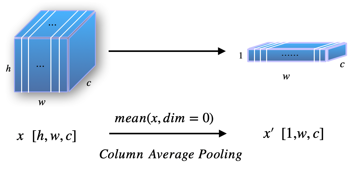
Suppose the size of feature map of the last layer has shape: , where are the height, width and the number of channels respectively. Here, we omit the batch dimension. CAP is really simple, let be the output of CAP, then
| (1) |
3.2 MultiRow Stretching
In order to tackle with multi-row images, we first use one simple method to stretch final layer’s feature map into one row. Inspired by FCN in objection detection (Dai et al. (2016)), each sliding window can be processed in parallel using conv operation, so the final layer’s feature map can be decomposed into different parts corresponding to each window. For multi-row images, each row can be operated in parallel as well, therefore, we adopt the same idea from FCN, using the same architecture for recognizing single-row images, we can derive multi-row feature map in the last layer illustrated in Figure 2, so we reshape it into a single row feature map in MultiRow Stretching method.
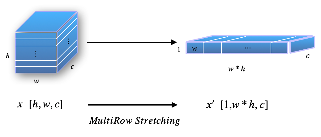
Intuitively, we treat all sentences in one image as one sentence by concatenating them together in row manner. Specifically, reuse the notation from above section, to calculate CTC loss finally, we do the following operations in PyTorch fashion with label :
| (2) | ||||
| (3) |
3.3 Attention
MultiRow Stretching can tackle with images with few characters, the vanishing or exploding gradient problem may occur if the stretched features are long. Moreover, if there is no evident relationship among each row in the original input image, then this method may converge to sub-optimal result. Therefore, we use similar attention method from ECANet (Wang et al. (2020)) to derive final feature map for image with fixed rows. Figure 3 illustrates this procedure.
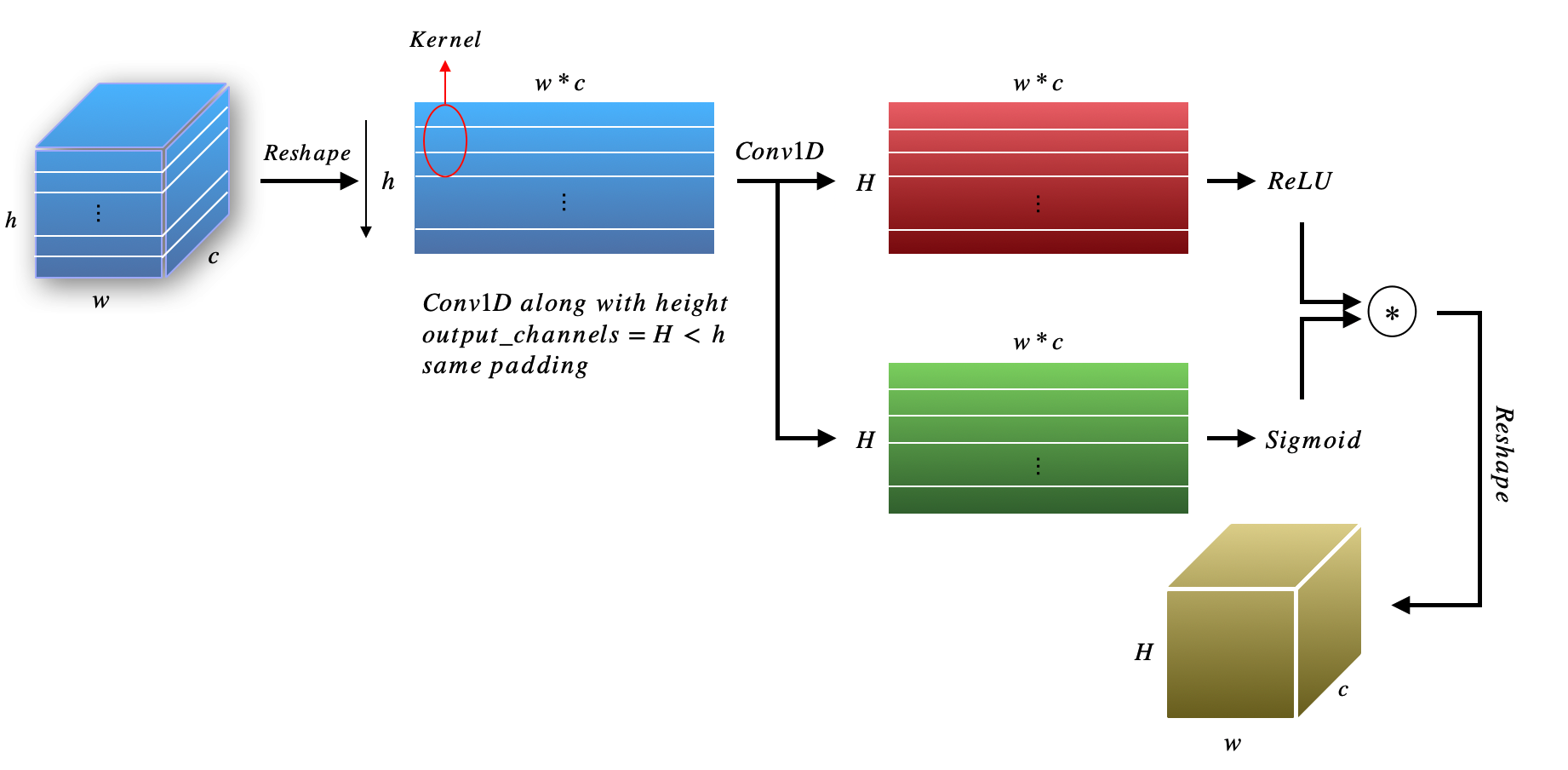
Following the above notations, we first reshape 3D tensor into 2D tensor . For each row of feature, we treat it as one element of final feature map. Intuitively, suppose the rows of each image is , so we attend each row in to derive both feature map and sigmoidal attention mask. Like in ECANet, we use Conv1D to conv over the height of feature map. Final results can be derived by the product of attended feature maps and attention masks. To summarize the above statement, we have the following operations:
| (4) | ||||
| (5) | ||||
| (6) | ||||
| (7) | ||||
| (8) | ||||
| (9) |
For final , we separate it into independent parts row by row. Then we input them into BiLSTM to calculate individual CTC loss. Given batch size , the optimized CTC loss is :
| (10) |
where is the example of part of feature map, is the corresponding label.
3.4 Line-Deep Denoising Convolutional AutoEncoder
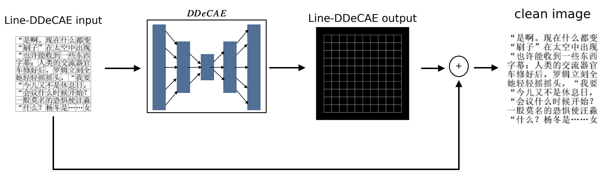
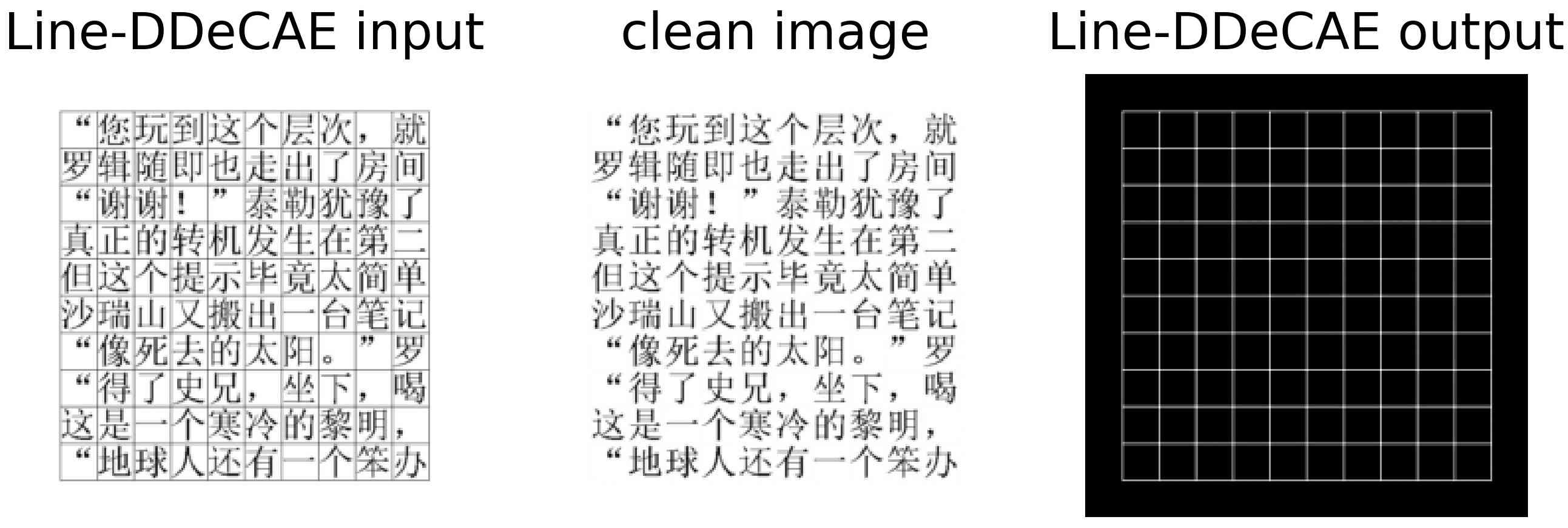
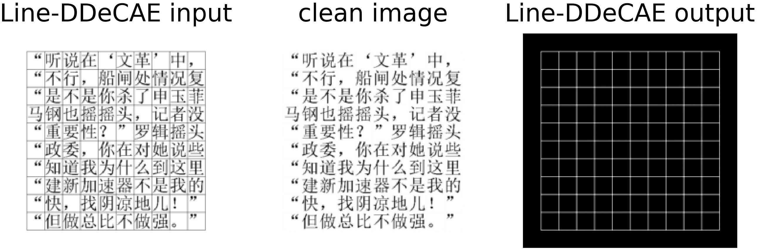
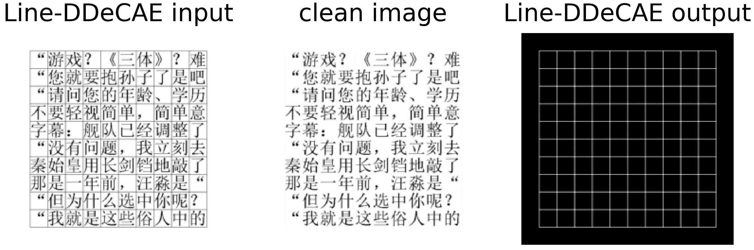
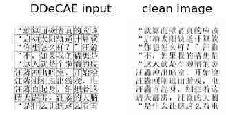
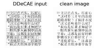
In this section, we propose one Deep Denoising Convolutional AutoEncoder(DDeCAE) (Gondara (2016)) variant, called Line-DDeCAE in Figure 4 to strip away box lines in the original images. Original images with excel-like form are harder to recognize. Therefore, in this work, we tend to first obtain clean images without box lines, then send them into CRNN to do recognition task.
Inspired by Denoising AutoEncoder(DeAE), the original input is distorted by a small random noise to be compressed into tight features and reconstruct the original input. Intuitively, adding noise lets original data distribution draft away a little, which lead to more robust compressed features. In this work, we either treat texts in the image as noise trying to recover box lines or box lines in the image as noise trying to recover texts(which is what DDeCAE does). We use the same architectures in DCGAN’s (Radford et al. (2015)) discriminator and generator to construct Line-DDeCAE’s encoder and decoder respectively with few modifications.
In experiments, we find when we treat box lines as noise and recover texts, the results are really noisy. Since texts lie in the more complicated manifold in high dimension than box lines, therefore stripping box lines is one easier task, recovering texts is harder. As a result, we try to recover box lines with texts being noise. Recall in original DeAE, authors recommended noisy inputs should not drift too much from original data distribution. In Line-DDeCAE, we evidently let noise be really different from original manifold. However, in experiments, we find this method works quite well. We assume that though noise(texts) is far from original manifold(box lines), box lines lie in more compact manifold and recovering it from higher manifold is relatively easy. Finally, we add original input image with Line-DDeCAE’s output in order to get clean images without box lines.
In conclusion, suppose the original input with box lines is , the Line-DDeCAE’s output is , then clean image is , the above procedure can be summed up in the following operations:
| (11) | ||||
| (12) |
3.5 Knowledge Distillation
In this section, we introduce one simple KD method for compressing large(teacher) CRNN model into a small(student) one.
Standard KD uses KL divergence to push student’s softmax to be close to teacher’s with temperature hyperpatameter , which is called soft target. Concretely, standard KD applies loss function combined soft targets with original targets(hard labels). Suppose the logit of teacher model is and logit of student model is and is corresponding ground-truth label, example’s softmax output of student model is , and softmax output of teacher model is , the loss of standard KD for student model is:
| (13) |
where is hyperparameter to trade off hard targets cross entropy loss and soft targets KL divergence.

In addition to standard KD, in CNN we also adopt the idea from FitNets (Romero et al. (2014)) to compare intermediate layers activations between teacher model and student model. In order to match the dimension, we use convolution layer as regressor layer. Assume we compare layers, for layer, the activation of student model is and the activation of teacher model is , then all layers MSE loss is:
| (14) |
Finally, to distill knowledge from BiLSTM as well, we propose to compare last time step of values and values between student model and teacher model because the last step of hidden values in BiLSTM may accumulate enough information to distill. Following the same notations above, denote last in teacher model as and student model as , we can write as:
| (15) |
We use the same hidden dimensions in both teacher model and student model.
To put it all together, we use the following loss function in optimization:
| (16) |
One thing to note that, we optimize the whole student model along with teacher model simultaneously, to overcome model collapse problem (Miyato et al. (2018)), we detach value of teacher model from PyTorch tensor to only encourage student model to be optimized towards distilled manner. Therefore the whole optimized loss function is :
| (17) |
As a whole, the KD algorithm proposed in this paper can be seen in Figure 5.
4 Experiments
4.1 Data Sets
In this paper, we generate simple synthetic data sets from a Chinese novel book: SanTi. We generate all samples following the order of the book. Each image includes 1 row or 7 rows or 10 rows and similar columns to make each image a near square shape except for single-row images. We create single-row images data set, called for CAP verification. For MultiRow Stretching and Attention methods, we generate (each image contains 7 rows) without box lines, and we also create multi-row images with box lines data set (each image contains 10 rows) to verify Line-DDeCAE method. For KD, we run on extended version of which is and for distillation.
For each method, we split corresponding data set into 80% for training and 20% for testing. Owing to the ease of CAP algorithm, we only generate 5,000 examples for training and testing. For MultiRow Stretching and Attention methods, we generate 30,000 examples overall. In KD, because we need to train teacher and student models at the same time, we ought to enlarge to 10,000 examples with more characters in each image. Table 1 summarizes statistics of the data sets for different methods and Figure 6 gives sampled examples from data sets to illustrate data set styles.
| data set | verified methods | # examples | # train | # test | # rows |
|---|---|---|---|---|---|
| CAP | 5,000 | 4,000 | 1,000 | 1 | |
| KD | 10,000 | 8,000 | 2,000 | 1 | |
| MultiRow Stretching/Attention/KD | 30,000 | 24,000 | 6,000 | 7 | |
| Line-DDeCAE | 30,000 | 24,000 | 6,000 | 10 |
4.2 Implementation
During training, we resize the input image into for single-row images and for multi-row images, we also turn all RGB images into gray scale. In CNN module, we follow the same hyperparameters setting in original VGG16 model but cut a few layers off to avoid overfitting except in the last pooling layer, we use pool size of (2, 3) for single-row images. In BiLSTM module, we set hidden size to be 256 and stack 2 BiLSTM layers. During training, for most of experiments, we set training epochs to be 200 with batch size 16, we try SGD optimizer with Nesterov mode with momentum 0.9 and we also try Adam with AMSGrad mode with momentum 0.9 and RMSProp 0.99, but we only report superior SGD results in single-row images and superior Adam results in multi-row images. Initial learning rate is set with decay rate of 2 for every 60 epochs. We also set weight decay parameter to be . In KD, with parameter being 0.5 and with parameter being 0.2, we set temperature to be 1.5, we obtain above hyperparameters with grid search by spliting training data into 90% training and 10% validation. For student model, we cut off a few layers in CNN module and only use one layer of BiLSTM. More details with hyperparameters can be found in Appendix A.1.
4.3 Metrics
In this paper, we use two metrics: character-level precision(CLP) and image-level precision(ILP). In CLP, we count predicted characters in each image against all characters, in ILP, if all characters in each image are predicted correctly, we get one right result. Concretely,
| (18) | |||
| (19) |
where is the number of examples and is the number of characters in example, is ground-truth and is the corresponding prediction, is indicator function.
4.4 Results
We report all averaged results on test set with three runs each.
4.4.1 CAP
In this part, we use to compare CAP with original CRNN model. In table 2, as comparison, we use the default setting in CRNN model. Notice CAP performs almost equally to original CRNN model both in CLP(-0.09%) and ILP(-0.08%). We argue that CAP can also obtain similar results without hand tuning hyperparameters in CNN module.
| methods | CLP | ILP |
|---|---|---|
| CRNN | 97.31 | 91.33 |
| CAP | 97.20 | 91.25 |
4.4.2 MultiRow Stretching and Attention
We use without box lines to verify both MultiRow Stretching and Attention methods. Final results are in Table 3. Original CRNN can’t handle multi-row images, hence we only report two proposed methods. Note that for MultiRow Stretching final results are pretty good compared to Attention method in CLP(+0.76%), we argue the data set contains only 7-row images, we claim this performance may decline if each image contains more rows.
| methods | CLP | ILP |
|---|---|---|
| MultiRow Stretching | 80.52 | 60.17 |
| Attention | 81.31 | 60.04 |
4.4.3 Line-DDeCAE
Next, we train Line-DDeCAE model using . The sampled images are in Figure 7, more samples can be found in the Appendix A.3. We also compared with simple DDeCAE model. Line-DDeCAE and DDeCAE share the same model structure. Note that, DDeCAE model fails to recover texts well, however, Line-DDeCAE recovers box lines almost perfectly. We also conclude that Line-DDeCAE also converges faster and better than DDeCAE, training procedures can be found in Appendix A.2. Then, to verify more Line-DDeCAE model, we input data into pre-trained Line-DDeCAE model and inject output into CRNN model to train MultiRow Stretching algorithm. All results are in Table 4. Compared to DDeCAE we notice that, using Line-DDeCAE can obtain high performance both in CLP(+5.09%) and ILP(+9.51%). Also notice that if we directly input into CRNN, the model fails to converge at certain level.
| methods | CLP | ILP |
|---|---|---|
| CRNN | 50.77 | 35.98 |
| DDeCAE+CRNN | 70.38 | 50.14 |
| Line-DDeCAE+CRNN | 75.47 | 59.65 |
4.4.4 KD
Finally, we use and to distill knowledge from previous teacher CRNN model into half-sized student CRNN model. To distill knowledge from teacher model efficiently, we train teacher and student model simultaneously. However, we detach values from tensors of teacher model to avoid model collapse problem (Miyato et al. (2018)). Final results can be found in Table 5. In single-row images, performance was improved by a huge gap(+2.45% in CLP, +7.03% in ILP) in distilled model, and in multi-row images, we run MultiRow Stretching method, distilled model still outperforms teacher model(+0.22% in CLP, +0.23% in ILP). In summary, almost half of parameters are reduced, but similar accuracy is retained and even boosted, which is a very promising result.
| data sets | methods | CLP | ILP |
|---|---|---|---|
| CRNN | 89.29 | 71.17 | |
| Distilled CRNN | 91.74 | 78.20 | |
| CRNN(MultiRow Stretching) | 80.52 | 60.17 | |
| Distilled CRNN | 80.74 | 60.40 |
5 Conclusion
In this paper, we’ve proposed multiple simple yet effective methods to boost CRNN performance via implementing Chinese text images recognition task. In particular, we advocated to use CAP to replace exhaustive hyperparameters fine-tuning with single-row images; we also proposed two methods to tackle with multi-row images; original CRNN can’t recognize excel-like images well, we thus proposed Line-DDeCAE to first recover box lines, which we found is an easy task, then add original input image to obtain clean image; finally, we proposed efficient online KD method to distill teacher model into half-sized student model without loss of generality. Experimental results on generated synthetic data set revealed our methods being of high efficiency.
References
- Bahdanau et al. (2014) Dzmitry Bahdanau, Kyunghyun Cho, and Yoshua Bengio. Neural machine translation by jointly learning to align and translate. arXiv preprint arXiv:1409.0473, 2014.
- Bissacco et al. (2013) Alessandro Bissacco, Mark Cummins, Yuval Netzer, and Hartmut Neven. Photoocr: Reading text in uncontrolled conditions. In Proceedings of the IEEE International Conference on Computer Vision, pp. 785–792, 2013.
- Chen et al. (2017) Guobin Chen, Wongun Choi, Xiang Yu, Tony Han, and Manmohan Chandraker. Learning efficient object detection models with knowledge distillation. In Advances in Neural Information Processing Systems, pp. 742–751, 2017.
- Dai et al. (2016) Jifeng Dai, Yi Li, Kaiming He, and Jian Sun. R-fcn: Object detection via region-based fully convolutional networks. In Advances in neural information processing systems, pp. 379–387, 2016.
- Dean et al. (2012) Jeffrey Dean, Greg Corrado, Rajat Monga, Kai Chen, Matthieu Devin, Mark Mao, Marc’aurelio Ranzato, Andrew Senior, Paul Tucker, Ke Yang, et al. Large scale distributed deep networks. In Advances in neural information processing systems, pp. 1223–1231, 2012.
- Devlin et al. (2018) Jacob Devlin, Ming-Wei Chang, Kenton Lee, and Kristina Toutanova. Bert: Pre-training of deep bidirectional transformers for language understanding. arXiv preprint arXiv:1810.04805, 2018.
- Fu et al. (2017) Jianlong Fu, Heliang Zheng, and Tao Mei. Look closer to see better: Recurrent attention convolutional neural network for fine-grained image recognition. In Proceedings of the IEEE conference on computer vision and pattern recognition, pp. 4438–4446, 2017.
- Girshick et al. (2014) Ross Girshick, Jeff Donahue, Trevor Darrell, and Jitendra Malik. Rich feature hierarchies for accurate object detection and semantic segmentation. In Proceedings of the IEEE conference on computer vision and pattern recognition, pp. 580–587, 2014.
- Gondara (2016) Lovedeep Gondara. Medical image denoising using convolutional denoising autoencoders. In 2016 IEEE 16th International Conference on Data Mining Workshops (ICDMW), pp. 241–246. IEEE, 2016.
- Graves et al. (2008) Alex Graves, Marcus Liwicki, Santiago Fernández, Roman Bertolami, Horst Bunke, and Jürgen Schmidhuber. A novel connectionist system for unconstrained handwriting recognition. IEEE transactions on pattern analysis and machine intelligence, 31(5):855–868, 2008.
- Han et al. (2015a) Song Han, Huizi Mao, and William J Dally. Deep compression: Compressing deep neural networks with pruning, trained quantization and huffman coding. arXiv preprint arXiv:1510.00149, 2015a.
- Han et al. (2015b) Song Han, Jeff Pool, John Tran, and William Dally. Learning both weights and connections for efficient neural network. In Advances in neural information processing systems, pp. 1135–1143, 2015b.
- Hinton et al. (2015) Geoffrey Hinton, Oriol Vinyals, and Jeff Dean. Distilling the knowledge in a neural network. arXiv preprint arXiv:1503.02531, 2015.
- Hu et al. (2018) Jie Hu, Li Shen, and Gang Sun. Squeeze-and-excitation networks. In Proceedings of the IEEE conference on computer vision and pattern recognition, pp. 7132–7141, 2018.
- Hubara et al. (2016) Itay Hubara, Matthieu Courbariaux, Daniel Soudry, Ran El-Yaniv, and Yoshua Bengio. Binarized neural networks. In Advances in neural information processing systems, pp. 4107–4115, 2016.
- Iandola et al. (2016) Forrest N Iandola, Song Han, Matthew W Moskewicz, Khalid Ashraf, William J Dally, and Kurt Keutzer. Squeezenet: Alexnet-level accuracy with 50x fewer parameters and¡ 0.5 mb model size. arXiv preprint arXiv:1602.07360, 2016.
- Jaderberg et al. (2016) Max Jaderberg, Karen Simonyan, Andrea Vedaldi, and Andrew Zisserman. Reading text in the wild with convolutional neural networks. International journal of computer vision, 116(1):1–20, 2016.
- Kao et al. (2018) Chieh-Chi Kao, Weiran Wang, Ming Sun, and Chao Wang. R-crnn: Region-based convolutional recurrent neural network for audio event detection. arXiv preprint arXiv:1808.06627, 2018.
- Kapka & Lewandowski (2019) Sławomir Kapka and Mateusz Lewandowski. Sound source detection, localization and classification using consecutive ensemble of crnn models. arXiv preprint arXiv:1908.00766, 2019.
- Khandelwal et al. (2019) Urvashi Khandelwal, Kevin Clark, Dan Jurafsky, and Lukasz Kaiser. Sample efficient text summarization using a single pre-trained transformer. arXiv preprint arXiv:1905.08836, 2019.
- Kingma & Welling (2013) Diederik P Kingma and Max Welling. Auto-encoding variational bayes. arXiv preprint arXiv:1312.6114, 2013.
- Li et al. (2016) Hao Li, Asim Kadav, Igor Durdanovic, Hanan Samet, and Hans Peter Graf. Pruning filters for efficient convnets. arXiv preprint arXiv:1608.08710, 2016.
- Li et al. (2018) Xiang Li, Wenhai Wang, Wenbo Hou, Ruo-Ze Liu, Tong Lu, and Jian Yang. Shape robust text detection with progressive scale expansion network. arXiv preprint arXiv:1806.02559, 2018.
- Li et al. (2019) Xiang Li, Wenhai Wang, Xiaolin Hu, and Jian Yang. Selective kernel networks. In Proceedings of the IEEE conference on computer vision and pattern recognition, pp. 510–519, 2019.
- Luo et al. (2017) Jian-Hao Luo, Jianxin Wu, and Weiyao Lin. Thinet: A filter level pruning method for deep neural network compression. In Proceedings of the IEEE international conference on computer vision, pp. 5058–5066, 2017.
- Miyato et al. (2018) Takeru Miyato, Shin-ichi Maeda, Masanori Koyama, and Shin Ishii. Virtual adversarial training: a regularization method for supervised and semi-supervised learning. IEEE transactions on pattern analysis and machine intelligence, 41(8):1979–1993, 2018.
- Molchanov et al. (2016) Pavlo Molchanov, Stephen Tyree, Tero Karras, Timo Aila, and Jan Kautz. Pruning convolutional neural networks for resource efficient inference. arXiv preprint arXiv:1611.06440, 2016.
- Ng et al. (2011) Andrew Ng et al. Sparse autoencoder. CS294A Lecture notes, 72(2011):1–19, 2011.
- Radford et al. (2015) Alec Radford, Luke Metz, and Soumith Chintala. Unsupervised representation learning with deep convolutional generative adversarial networks. arXiv preprint arXiv:1511.06434, 2015.
- Raffel et al. (2019) Colin Raffel, Noam Shazeer, Adam Roberts, Katherine Lee, Sharan Narang, Michael Matena, Yanqi Zhou, Wei Li, and Peter J Liu. Exploring the limits of transfer learning with a unified text-to-text transformer. arXiv preprint arXiv:1910.10683, 2019.
- Rastegari et al. (2016) Mohammad Rastegari, Vicente Ordonez, Joseph Redmon, and Ali Farhadi. Xnor-net: Imagenet classification using binary convolutional neural networks. In European conference on computer vision, pp. 525–542. Springer, 2016.
- Redmon et al. (2016) Joseph Redmon, Santosh Divvala, Ross Girshick, and Ali Farhadi. You only look once: Unified, real-time object detection. In Proceedings of the IEEE conference on computer vision and pattern recognition, pp. 779–788, 2016.
- Ren et al. (2015) Shaoqing Ren, Kaiming He, Ross Girshick, and Jian Sun. Faster r-cnn: Towards real-time object detection with region proposal networks. In Advances in neural information processing systems, pp. 91–99, 2015.
- Rifai et al. (2011) Salah Rifai, Pascal Vincent, Xavier Muller, Xavier Glorot, and Yoshua Bengio. Contractive auto-encoders: Explicit invariance during feature extraction. In Icml, 2011.
- Romero et al. (2014) Adriana Romero, Nicolas Ballas, Samira Ebrahimi Kahou, Antoine Chassang, Carlo Gatta, and Yoshua Bengio. Fitnets: Hints for thin deep nets. arXiv preprint arXiv:1412.6550, 2014.
- Sandler et al. (2018) Mark Sandler, Andrew Howard, Menglong Zhu, Andrey Zhmoginov, and Liang-Chieh Chen. Mobilenetv2: Inverted residuals and linear bottlenecks. In Proceedings of the IEEE conference on computer vision and pattern recognition, pp. 4510–4520, 2018.
- Shi et al. (2016) Baoguang Shi, Xiang Bai, and Cong Yao. An end-to-end trainable neural network for image-based sequence recognition and its application to scene text recognition. IEEE transactions on pattern analysis and machine intelligence, 39(11):2298–2304, 2016.
- Simonyan & Zisserman (2014) Karen Simonyan and Andrew Zisserman. Very deep convolutional networks for large-scale image recognition. arXiv preprint arXiv:1409.1556, 2014.
- Vaswani et al. (2017) Ashish Vaswani, Noam Shazeer, Niki Parmar, Jakob Uszkoreit, Llion Jones, Aidan N Gomez, Łukasz Kaiser, and Illia Polosukhin. Attention is all you need. In Advances in neural information processing systems, pp. 5998–6008, 2017.
- Wang et al. (2020) Qilong Wang, Banggu Wu, Pengfei Zhu, Peihua Li, Wangmeng Zuo, and Qinghua Hu. Eca-net: Efficient channel attention for deep convolutional neural networks. In Proceedings of the IEEE/CVF Conference on Computer Vision and Pattern Recognition, pp. 11534–11542, 2020.
- Wang et al. (2012) Tao Wang, David J Wu, Adam Coates, and Andrew Y Ng. End-to-end text recognition with convolutional neural networks. In Proceedings of the 21st international conference on pattern recognition (ICPR2012), pp. 3304–3308. IEEE, 2012.
- Wu et al. (2016) Jiaxiang Wu, Cong Leng, Yuhang Wang, Qinghao Hu, and Jian Cheng. Quantized convolutional neural networks for mobile devices. In Proceedings of the IEEE Conference on Computer Vision and Pattern Recognition, pp. 4820–4828, 2016.
- Yim et al. (2017) Junho Yim, Donggyu Joo, Jihoon Bae, and Junmo Kim. A gift from knowledge distillation: Fast optimization, network minimization and transfer learning. In Proceedings of the IEEE Conference on Computer Vision and Pattern Recognition, pp. 4133–4141, 2017.
- Zagoruyko & Komodakis (2016) Sergey Zagoruyko and Nikos Komodakis. Paying more attention to attention: Improving the performance of convolutional neural networks via attention transfer. arXiv preprint arXiv:1612.03928, 2016.
- Zhang et al. (2019) Linfeng Zhang, Jiebo Song, Anni Gao, Jingwei Chen, Chenglong Bao, and Kaisheng Ma. Be your own teacher: Improve the performance of convolutional neural networks via self distillation. In Proceedings of the IEEE International Conference on Computer Vision, pp. 3713–3722, 2019.
- Zhang et al. (2018a) Xiangyu Zhang, Xinyu Zhou, Mengxiao Lin, and Jian Sun. Shufflenet: An extremely efficient convolutional neural network for mobile devices. In Proceedings of the IEEE conference on computer vision and pattern recognition, pp. 6848–6856, 2018a.
- Zhang et al. (2018b) Ying Zhang, Tao Xiang, Timothy M Hospedales, and Huchuan Lu. Deep mutual learning. In Proceedings of the IEEE Conference on Computer Vision and Pattern Recognition, pp. 4320–4328, 2018b.
- Zhou et al. (2020) Zaida Zhou, Chaoran Zhuge, Xinwei Guan, and Wen Liu. Channel distillation: Channel-wise attention for knowledge distillation. arXiv preprint arXiv:2006.01683, 2020.
Appendix A Appendix
A.1 Training Hyperparameters
In this section, we list all hyperparameters in all experiments in Table 6.
| methods | hyperparameters | ||||
| image size | epochs | batch size | optimizer | init_lr | |
| CRNN | (224, 224)/(64, 128) | 200 | 20 | AMSGrad/Nesterov | 1e-4 |
| CAP | (64, 128) | 200 | 20 | Nesterov | 1e-4 |
| MultiRow Stretching | (224, 224) | 200 | 20 | AMSGrad | 1e-4 |
| Attention | (224, 224) | 200 | 20 | AMSGrad | 1e-4 |
| DDeCAE | (224, 224) | 100 | 64 | Adam | 1e-3 |
| Line-DDeCAE | (224, 224) | 100 | 64 | Adam | 1e-3 |
| DDeCAE + CRNN | (224, 224) | 200 | 16 | AMSGrad | 1e-4 |
| Line-DDeCAE + CRNN | (224, 224) | 200 | 16 | AMSGrad | 1e-4 |
| KD with single-row | (64, 128) | 300 | 16 | Nesterov | 1e-4 |
| KD with multi-row | (224, 224) | 300 | 16 | AMSGrad | 1e-4 |
| lr_decay rate | weight decay | temperature | |||
| CRNN | 2 | 1e-6 | N/A | N/A | N/A |
| CAP | 2 | 1e-6 | N/A | N/A | N/A |
| MultiRow Stretching | 2 | 1e-6 | N/A | N/A | N/A |
| Attention | 2 | 1e-6 | N/A | N/A | N/A |
| DDeCAE | 5 | 0 | N/A | N/A | N/A |
| Line-DDeCAE | 5 | 0 | N/A | N/A | N/A |
| DDeCAE + CRNN | 2 | 1e-6 | N/A | N/A | N/A |
| Line-DDeCAE + CRNN | 2 | 1e-6 | N/A | N/A | N/A |
| KD with single-row | 2 | 1e-6 | 0.5 | 0.2 | 1.5 |
| KD with multi-row | 2 | 1e-6 | 0.5 | 0.2 | 1.5 |
In the table, init_lr means initial learning rate, lr_rate means learning rate decay rate, and are hyperparameters to trade off between and .
A.2 Training Procedures in Line-DDeCAE and DDeCAE
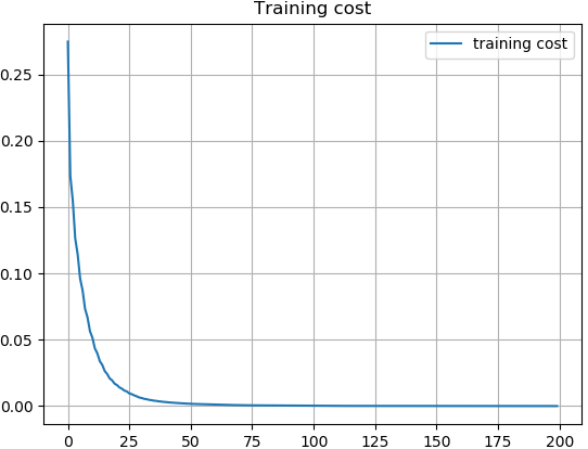
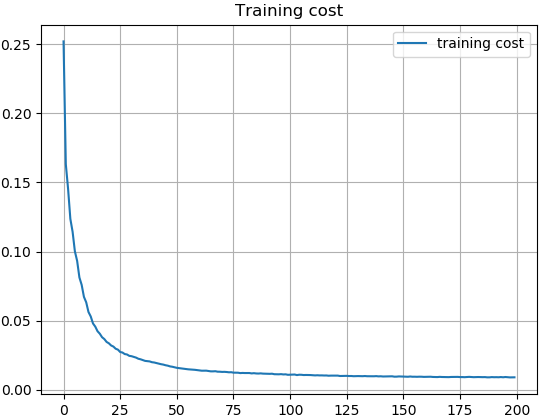
Figure 8 reveals how training losses change both in Line-DDeCAE and DDeCAE, we can see Line-DDeCAE converges slightly faster and much better than DDeCAE, we argue that since box lines are easily to be recovered in high dimensional space than texts, therefore, Line-DDeCAE is a reasonable alternative in this scenario.
A.3 More Samples from Line-DDeCAE and DDeCAE
In this section, we display more results on Line-DDeCAE and DDeCAE for comparison in Figure 9 and Figure 10 respectively.
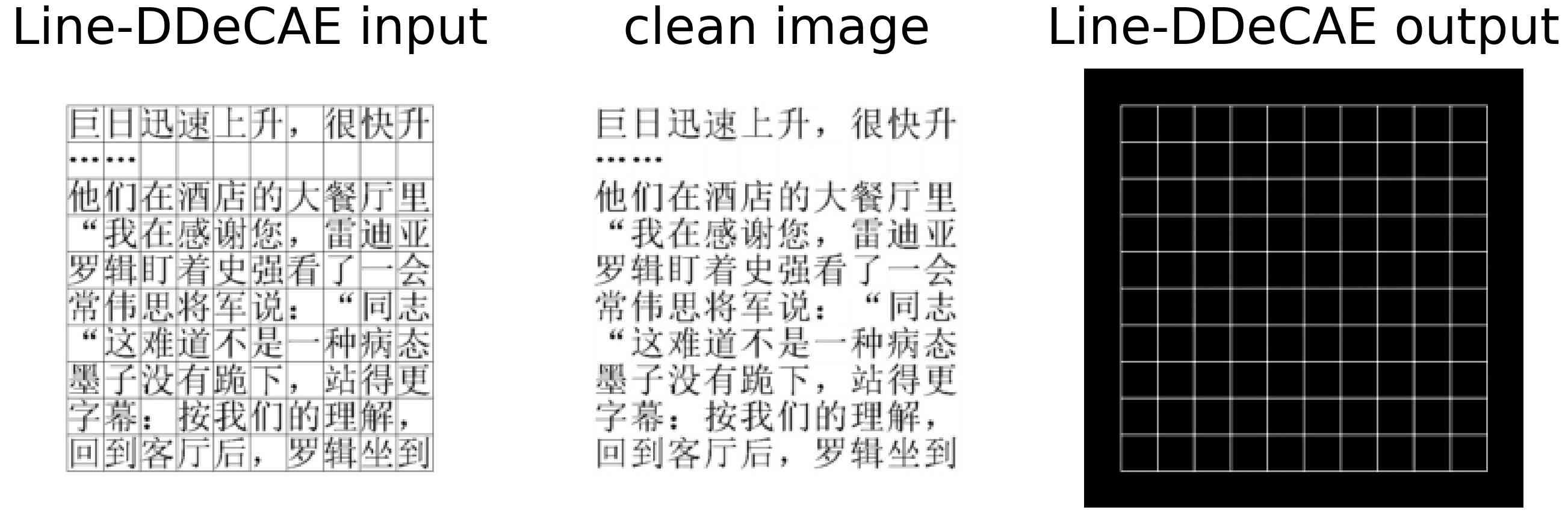
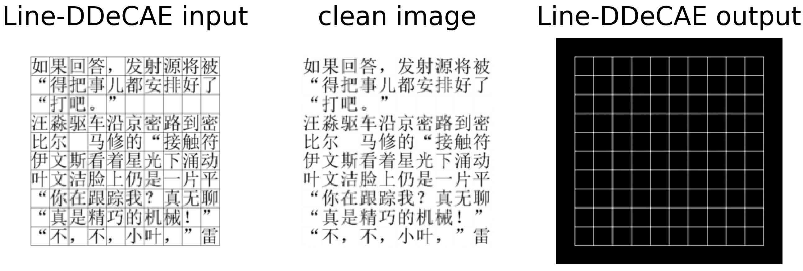
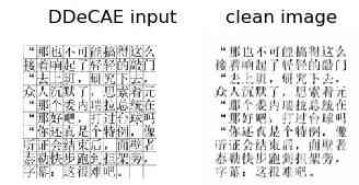
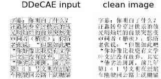

According to figures, we conclude that Line-DDeCAE explicitly recovers box lines perfectly, whereas DDeCAE tries harder to recover texts which is not ideal.