Adaptable Hamiltonian neural networks

Abstract

The rapid growth of research in exploiting machine learning to predict chaotic systems has revived a recent interest in Hamiltonian Neural Networks (HNNs) with physical constraints defined by the Hamilton’s equations of motion, which represent a major class of physics-enhanced neural networks. We introduce a class of HNNs capable of adaptable prediction of nonlinear physical systems: by training the neural network based on time series from a small number of bifurcation-parameter values of the target Hamiltonian system, the HNN can predict the dynamical states at other parameter values, where the network has not been exposed to any information about the system at these parameter values. The architecture of the HNN differs from the previous ones in that we incorporate an input parameter channel, rendering the HNN parameter–cognizant. We demonstrate, using paradigmatic Hamiltonian systems, that training the HNN using time series from as few as four parameter values bestows the neural machine with the ability to predict the state of the target system in an entire parameter interval. Utilizing the ensemble maximum Lyapunov exponent and the alignment index as indicators, we show that our parameter-cognizant HNN can successfully predict the route of transition to chaos. Physics-enhanced machine learning is a forefront area of research, and our adaptable HNNs provide an approach to understanding machine learning with broad applications.

I Introduction

A daunting challenge in machine learning is the lack of understanding of the inner working of the artificial neural networks. As machine learning has been increasingly incorporated into many vital structures and systems that support the functioning of the modern society, it is imperative to develop a general understanding of the inner gears of the underlying neural networks. For example, feed-forward neural networks or multilayer perceptrons constitute the fundamentals of modern deep learning machines with broad applications in image, video and audio processing LeCun et al. (2015). Such a neural machine typically consists of an input layer, a large number of hidden layers, and an output layer. From the input layer on, nodes in the same layer do not interact with each other, but they are connected with the nodes in the next layer via a set of weights and biases whose values are determined through training, where the paradigmatic method of stochastic gradient descent (SGD) Goodfellow et al. (2016) is often used. How the networks in different layers work together to solve a specific problem remains unknown. In another line of research, reservoir computing, a class of recurrent neural networks Jaeger (2001); Mass et al. (2002); Jaeger and Haas (2004); Manjunath and Jaeger (2013), has gained considerable momentum since 2017 as a powerful paradigm for model-free, fully data driven prediction of nonlinear and chaotic dynamical systems Haynes et al. (2015); Larger et al. (2017); Pathak et al. (2017); Lu et al. (2017); Duriez et al. (2017); Lu et al. (2018); Pathak et al. (2018a, b); Carroll (2018); Nakai and Saiki (2018); Roland and Parlitz (2018); Weng et al. (2019); Griffith et al. (2019); Jiang and Lai (2019); Vlachas et al. (2019); Fan et al. (2020); Zhang et al. (2020). A reservoir computing machine constitutes an input layer, a single hidden layer, and an output layer. Differing from the network structure of a multilayer perceptron, the network in the hidden layer of a reservoir computing machine has a complex topology in which the nodes are coupled with each other following some probability distribution. Another difference is that, in feed-forward neural networks, only the weights and biases connecting the hidden layer and the output layer neurons are determined by training, while in reservoir computing those parameters as well as the weights of the complex network in the hidden layer are pre-defined. A well trained reservoir machine can generate accurate prediction of the state evolution of a chaotic system for a duration that is typically several times longer than that which can be achieved using the traditional methodologies in nonlinear time series analysis. This is remarkable, considering the hallmark of chaos: sensitive dependence on initial conditions, which rules out long-term prediction. Yet, there is little understanding of how the internal network dynamics of reservoir computing machines behave or “manage” to replicate accurately (for some amount of time) the chaotic evolution of the true system.

At the present, to develop a general explainable framework to encompass various types of machine learning is not feasible. In this regard, a promising direction of pursuit is the so-called physics-enhanced machine learning, in which the neural networks are designed to solve specific physics problems with the goal to enhance the learning efficiency through exploiting the underlying physical principles or constraints. The idea was articulated almost three decades ago De Wilde (1993), when the principle of Hamiltonian mechanics was incorporated into the design of neural networks, leading to Hamiltonian Neural Networks (HNNs) that have recently gained renewed attention Greydanus et al. (2019); Toth et al. (2019); Bertalan et al. (2019); Choudhary et al. (2020a); Garg and Kagi (2019). Comparing with traditional neural networks, in an HNN, the energy is conserved. It has been demonstrated that, an HNN can be trained to possess the power to predict the dynamical evolution of the target Hamiltonian system in both integrable and chaotic regimes, provided that the network is trained with data taken from the same set of parameter values at which the prediction is to be made Greydanus et al. (2019); Toth et al. (2019); Bertalan et al. (2019); Choudhary et al. (2020a); Garg and Kagi (2019). Recently the principle of HNN has been generalized Chen et al. (2019) to systems described by the Lagrangian equation of motion Cranmer et al. (2020) and a general type of ordinary differential equations Sanchez-Gonzalez et al. (2019) or coordinate transforms Dulberg and Cohen (2020); Choudhary et al. (2020b) with applications in robotics Lutter et al. (2019); Havoutis and Ramamoorthy (2010).

In this paper, we address adaptability, a fundamental issue in machine learning, of Hamiltonian neural networks. More precisely, we consider the situation where a target Hamiltonian system can experience slow drift or sudden changes in some parameters. Slow environmental variations can lead to adiabatic parameter drifting, while external disturbances can lead to sudden parameter changes. We ask if it is possible to design HNNs, which are trained with data from a small number of parameter values of the target system, to have the predictive power for parameter values that are not in the training set. Inspired by the recent work on predicting critical transitions and collapse in dissipative dynamical systems based on reservoir computing Falahian et al. (2015); Cestnik and Abel (2019); Kim et al. (2020); Klos et al. (2020); Kong et al. (2021), we articulate a class of HNNs whose input layer contains a set of channels that are specifically used for inputting the values of the distinct parameters of interest to the neural network. The number of the parameter channels is equal to the number of freely varying parameters in the target Hamiltonian system. The simplest case is where the target system has a single bifurcation or control parameter so only one input parameter channel to the neural network is necessary. We demonstrate that, by incorporating such a parameter channel into a feed-forward type of HNNs and conducting training using time series data from a small number of bifurcation parameter values (e.g., four), we effectively make the HNN adaptable to parameter variations. That is, the so-trained HNN has inherited the rules governing the dynamical evolution of the target Hamiltonian system. When a parameter value of interest, which is not in the training parameter set, is fed into the HNN through the parameter channel, the machine is capable of generating dynamical behaviors that statistically match those of the target system at this particular parameter value. The HNN has thus become adaptable because it has never been exposed to any information or data from the target system at this parameter value, yet the neural machine can reproduce the dynamical behavior. Using the Hénon-Heiles model as a prototypical target Hamiltonian system, we demonstrate that our adaptable HNN can successfully predict the dynamical behaviors, integrable or chaotic, for any parameter values that are reasonably close to those in the training parameter set. Remarkably, by feeding a systematically varying set of bifurcation parameter values into the parameter channel, the HNN can successfully predict the transition to chaos in the target Hamiltonian system, which we characterize using two measures: the ensemble maximum Lyapunov exponent and the alignment index. It is worth emphasizing that, in the existing literature on HNNs Greydanus et al. (2019); Toth et al. (2019); Bertalan et al. (2019); Choudhary et al. (2020a); Garg and Kagi (2019), training and prediction are done at the same set of parameter values of the target Hamiltonian system, but our work goes beyond by making the HNN significantly more powerful with enhanced and expanded predictability.

We remark that, in physics, machine learning has been exploited to solve difficult problems in particle physics Guest et al. (2018); Radovic et al. (2018), quantum many-body systems Carleo and Troyer (2017), inverse design in optical systems Peurifoy et al. (2018), and quantum information Dunjko and Briegel (2018); Carleo et al. (2019). However, the working mechanisms of the underlying neural networks remain largely unknown Iten et al. (2020). The physics enhanced HNNs studied here are different from these applications, as we focus on exploiting physical principles to enable neural networks with unprecedented predictive power with respect to parameter variations.

In Sec. II, we describe the architecture of the articulated parameter-cognizant HNNs and the method of training. In Sec. III, we present results of predicting the dynamical behavior of the Hénon-Heiles system in a wide parameter region, including the transition to chaos based on calculating the ensemble maximum Lyapunov exponent and the minimum alignment index. In general, the prediction accuracy depends on how “close” the desired parameter value is to the training regime. In Sec. IV, we address a number of pertinent issues such as the choosing of the training parameter values, multiple parameter channels, and HNNs for a Hamiltonian system defined by the one-dimensional Morse potential. A summarizing discussion and speculations are offered in Sec. V.

II Parameter-cognizant Hamiltonian neural networks

The central idea for physics-enhanced machine learning is to “force” the dynamical evolution of the neural network to follow certain physical rules or constraints, examples of which are Hamilton’s equations of motion Greydanus et al. (2019); Toth et al. (2019); Bertalan et al. (2019); Choudhary et al. (2020a); Garg and Kagi (2019), Lagrangian equations Cranmer et al. (2020), or the principle of least action Karkar et al. (2020); Yang et al. (2020). In particular, the structure of HNNs is such that the underlying neural dynamical system is effectively a Hamiltonian system for which the energy is conserved during the evolution. Different from previous work Greydanus et al. (2019); Toth et al. (2019); Bertalan et al. (2019); Choudhary et al. (2020a); Garg and Kagi (2019), the bifurcation parameter of the target Hamiltonian system serves as an input “variable” to the neural network through an additional input channel so that the HNN learns to associate the input time series with the specific value of the bifurcation parameter. Using time series from a small number of distinct bifurcation parameter values to train the HNN, it can gain the ability to “sense” the changes in the dynamics (or dynamical “climate”) of the target system with the bifurcation parameter.

Figure 1: Structure of parameter-cognizant HNN. The input channels are denoted by the blue circles, which are connected to the first hidden layer (purple circles). The blue circle denoted by “$\alpha$” is the parameter input channel that feeds the value of the bifurcation parameter of the target Hamiltonian system, together with the time series $𝐪(t)$ and $𝐩(t)$ through the corresponding input channels, into the first hidden layer. There are two hidden layers. The output variables are the partial derivatives of the Hamiltonian of the target system with respect to the canonical coordinates and momenta, together with the Hamiltonian, which determine the dynamical state at the next time step.

The structure of our articulated parameter-cognizant HNN is shown in Fig. 1, where the input contains three parts: the position and momentum variables of the target system, and the bifurcation parameter. To be concrete, we use two hidden layers, where each layer contains $200$ artificial neurons (nodes). The third layer is the output, which contains a single node whose dynamical state corresponds to the Hamiltonian of the target system. Let $𝐲$ denote the set of dynamical variables of each layer. The transform from the dynamical variables in the $i$th layer to those in the $(i+1)$th layer follows the following rule:

$${𝐲}^{i+1}={𝝈}^i({𝒲}^i\cdot {𝐲}^i+{𝐛}^i),$$ (1)

where ${𝝈}^i$ is a given nonlinear activation function, ${𝒲}^i$ is the weight matrix and ${𝐛}^i$ is bias vector associated with the neurons in the $i$th layer, which are to be determined through training. We set the output as the spatial derivatives of the input variables to force the dynamics of the neural network to follow the Hamilton’s equations of motion. The derivatives are calculated through the back prorogation algorithm. Once the output is known, the loss function defined as

$$ℒ=\Vert \frac{\partial H}{\partial 𝐪}+\frac{d{𝐩}_{\text{real}}}{dt}\Vert +\Vert \frac{\partial H}{\partial 𝐩}-\frac{d{𝐪}_{\text{real}}}{dt}\Vert ,$$ (2)

can be calculated. Through the training process, we optimize the weights and biases in Eq. (1) by minimizing the loss function. This is done by using the standard SGD method Goodfellow et al. (2016). The whole process from network construction and training to carrying out the prediction is accomplished by using the open source package Tensorflow and Keras Abadi et al. (2016); Chollet et al. (2015).

Table 1 summarizes the structure and parameters of our HNN. It has about 40,000 unknown parameters to be optimally determined through training. The computation can be quite efficient even without using parallel or GPU acceleration. The anticipation is that, after training with time series data from a small number of distinct bifurcation parameter values, the HNN can predict the dynamical behavior of the target Hamiltonian system in a wide parameter interval, where the parameter variations are implemented through the input parameter channel to the HNN.

Table 1: Specifications of HNN

Description	Values
Number of hiden layers	$2$
Neurons per layer	$200$
Optimizer	Adam
Epochs	$500$
Activation functioin	tanh

Figure 2: Distinct types of dynamical behaviors in the Hénon-Heiles system. The energy value is $E=1/6$. (a-d) Integrable, mixed, small and largely chaotic dynamics for $\alpha =0$, 0.7, 0.9, and 1.0, respectively, on the Poincaré surface of section defined by $q_1=0$.

III Adaptable Hamiltonian neural networks for predicting transition to chaos

To test the adaptability of our parameter-cognizant HNN for predicting state evolution and dynamical transitions in Hamiltonian systems, we use the paradigmatic Hénon-Heiles model Hénon and Heiles (1964). It is a two-degrees-of-freedom system for investigating distinct types of Hamiltonian dynamics including integrable, mixed, and chaotic behaviors and the transitions among them. It was originated from the gravitational three-body system Hénon and Heiles (1964), with applications in contexts such as molecular dynamics Waite and Miller (1981); Feit and Fleck Jr (1984); Vendrell and Meyer (2011).

III.1 System description

The Hénon-Heiles Hamiltonian is

$$H=\frac{1}{2}\left(p_1^2+p_2^2\right)+\frac{1}{2}\left(q_1^2+q_2^2\right)+\alpha \left(q_1^2{q}_2-\frac{1}{3}{q}_2^3\right),$$ (3)

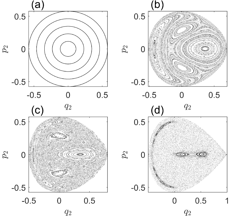
where $q_1$ and $q_2$ denote the coordinates, $p_1$ and $p_2$ are the corresponding momenta, $\alpha >0$ is a bifurcation parameter that sets the magnitude of the nonlinear potential function describing, e.g., the dissociation energy in molecules Waite and Miller (1981); Feit and Fleck Jr (1984); Vendrell and Meyer (2011). The dynamics of system Eq. (3) depend not only on $\alpha$, but also on the energy $E$ of the system that is conserved during the dynamical evolution. The maximum value of the potential function is $E_{\text{max}}=1/(6{\alpha }^2)$. For $\alpha =0$, $E_{\text{max}}$ diverges, so all trajectories are bounded. For $\alpha >0$, if the particle energy exceeds $E_{\text{max}}$, the Hamiltonian system becomes open with scattering trajectories that can escape to infinity. To train the adaptable HNN, bounded trajectories are required, so we set $0\le \alpha \le 1$ and $E\le 1/6$. (For particle energy above the threshold, chaotic scattering dynamics and fractal geometry can arise de Moura and Letelier (1999); Seoane et al. (2006, 2007).) As the value of $\alpha$ increases from zero to one, characteristically different dynamical behaviors can arise, such as integrable, mixed, and chaotic. In particular, for $\alpha =0$, the nonlinear term in Eq. (3) disappears and the system becomes a harmonic oscillator - an integrable system. In this case, the entire phase space contains periodic and quasiperiodic orbits only, as shown in Fig. 2(a). As $\alpha$ increases from zero, the system becomes nonlinear and chaotic seas amid the Kol’mogorov-Arnol’d-Moser (KAM) islands can arise in the phase space, giving rise to mixed dynamics, as shown in Fig. 2(b) for $\alpha =0.7$ and $E=1/6$. For $\alpha =0.9$, $\alpha =1$ and $E=1/6$, most trajectories in the phase space are chaotic, as shown in Figs. 2(c) and 2(d).

III.2 Training and testing of adaptability

Our goal of training is to “instill” certain adaptable power into the HNN. To achieve this, we choose a number of distinct values of the bifurcation parameter $\alpha$. For each $\alpha$ value, we randomly choose initial conditions with energy below the escape threshold $E_{\text{max}}$ and numerically integrate the Hamilton’s equations of motion to generate particle trajectories in the phase space. Because of the mixed dynamics, the training data contain both integrable and chaotic orbits. Specifically, the time interval of the trajectory is $0\le t\le 1000$, which contains hundreds of oscillation cycles, and we collect training data using the sampling time step $dt=0.1$. The energy associated with the training data is maintained to be constant to within ${10}^{-6}$.

In general, the weights and biases of the adaptable HNN determined by the SGD method depend on the training data set. To reduce the prediction error, an ensemble of HNNs can be used Kong et al. (2021). Concretely, for each value of $\alpha$, we generate $20$ different sets of data for training, leading to an ensemble of 20 HNNs. The parameter setting for training is listed in Tab. 2.

Table 2: List of training parameters for Hénon-Heiles system

Description	Values
Neural network ensembles	$20$
Energy samples	$7$
Orbit per energy	$1$
Orbit length	$1000$
Time step	$0.1$
Training parameter set	$\alpha \in \{0.2,0.4,0.6,0.8\}$

After the training, all the weights and biases in Eq. (1) are determined. The Hamiltonian and its derivatives for each network in the HNN ensemble can be evaluated for any input, leading to the average derivative values. To characterize the prediction accuracy for different values of the bifurcation parameter, we use the root-mean square error (RMSE) that can be calculated from the difference between the HNN predicted and the true orbits. For $\alpha =0$, the motion is integrable so the predicted orbit is always close to some real orbit, leading to exceedingly small errors. In this case, we take advantage of one feature of HNNs that it directly yields the Hamiltonian function, from which the potential function can be calculated. It is thus convenient to use the relative error between the predicted potential function and the true one to characterize the HNN performance, which is defined as

$$⟨\mathrm{\Delta }V⟩\equiv \frac{\overline{|V_{\text{pred}}-V_{\text{real}}|}}{\overline{V_{\text{real}}}},$$ (4)

where the average is taken in the region of . The predicted potential profile is given by $V_{\text{pred}}=H_{\text{pred}}-C$, where $C=\text{min}(H_{\text{pred}})$ so that the minimum value of $V_{\text{pred}}$ is zero. Note that the average in Eq. (4) is calculated from an integral in a 2D domain in the physical space, for which the boundary of the domain needs to be specified. A natural choice of the criterion to set the boundary would be , but occasionally the predicted orbit will diverge. Numerically, there are different ways to overcome this difficulty. For example, if the boundary is set according to the criterion: , then almost all orbits are bounded, rendering calculable the error $⟨\mathrm{\Delta }V⟩$.

We demonstrate that HNN can be used to reconstruct the Hamiltonian of the target system. Consider phase-space points for and expand the Hamiltonian about the origin using the Taylor series:

$$H_{\text{pred}}(\alpha )=\sum _{i_1,i_2,i_3,i_4}{\beta }_{i_1{i}_2{i}_3{i}_4}(\alpha )q_1^{i_1}{q}_2^{i_2}{p}_1^{i_3}{p}_2^{i_4},$$ (5)

where $\beta$’s are the expansion coefficients, and the sum is taken according to $0\le \text{sum}(i_1,i_2,i_3,i_4)\le 3$, which contains in total $35$ terms. Comparing with true Hamiltonian Eq. (3), only six terms are non-zero.

Figure 3: (a) Relative error in predicting the potential function of the Hénon-Heiles system. Shown is the error versus the bifurcation parameter $\alpha$ in the unit interval. The HNN is trained with time series data from four values of $\alpha$: $\alpha \in \{0.2,0.4,0.6,0.8\}$ (the four green pentagons). In the shaded region that contains these four values of $\alpha$, the relative error is less than $2\%$, demonstrating the adaptability of the HNN in predicting the target Hamiltonian system for parameter values not in the training set. The adaptability extends even outside the shaded region but with larger error (still within $8\%$ though). (b) Coefficients of the Taylor expansion for $H_{\text{pred}}$ versus the bifurcation parameter $\alpha$, where ${\beta }_{2000}$, ${\beta }_{0200}$, ${\beta }_{0020}$ and ${\beta }_{0002}$ correspond to the first four square terms in Eq. (3) whose true value is $1/2$, and ${\beta }_{2100}$ and ${\beta }_{0300}$ correspond to the two cubic terms that are proportional to $\alpha$. Other terms in the expansion do not appear in the original Hamiltonian, among which the first two largest ones are ${\beta }_{3000}$ and ${\beta }_{1200}$ that correspond to other cubic potential terms.

We train the HNN at four values of the bifurcation parameter: $\alpha \in \{0.2,0.4,0.6,0.8\}$. For each $\alpha$ value, we choose seven random initial conditions with their energies below the threshold. Figure 3(a) shows the relative error in predicting the potential function for $\alpha \in (0,1)$. The interval in $\alpha$ can be divided into two parts: the shaded region $\alpha \in [0.2,0.8]$ that contains the four values of $\alpha$ used in training, and the blank regions on both side of the shaded region. In the shaded region, the relative error is less than $2\%$, but the error increases away from the shaded region. Figure 3(b) shows the expansion coefficients for the predicted Hamiltonian. Comparing with the terms in the real Hamiltonian, our HNN predicts accurately the linear terms. For the nonlinear terms, the HNN reproduces the behavior with the variation in the bifurcation parameter $\alpha$, where the errors are small in the shaded region in Fig. 3(b) but relatively large outside the region.

Figure 4: Testing the adaptability of HNN for parameter values in between two training points. (a,b) True and predicted contour maps of the potential function for $\alpha =0.7$, respectively, where the latter is obtained by extracting the Hamiltonian at different positions with constant momentum input with normalization. (c,d) True and predicted orbits from the initial condition $[q_1,q_2,p_1,p_2]=[0,0,1/\sqrt{6},1/\sqrt{6}]$, respectively, which are quasiperiodic.

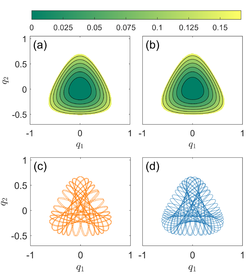
To examine the adaptability of our parameter-cognizant HNN in more detail, we take, for example, $\alpha =0.7$ in between the two training points $\alpha =0.6$ and $\alpha =0.8$, for which the vast majority of the orbits with energy $E=1/6$ are quasiperiodic, as can be seen from Fig. 2(b). Figures 4(a) and 4(b) show the true and predicted potential functions for , respectively, which are essentially indistinguishable. Figures 4(c) and 4(d) show some representative true and predicted orbits starting from the same initial condition, which agree with each other qualitatively but differ in detail. Particularly worth emphasizing is the fact that for the predicted quasiperiodic orbit, the energy can be maintained at a constant value. In fact, we have tested the method of reservoir computing Haynes et al. (2015); Larger et al. (2017); Pathak et al. (2017); Lu et al. (2017); Duriez et al. (2017); Lu et al. (2018); Pathak et al. (2018a, b); Carroll (2018); Nakai and Saiki (2018); Roland and Parlitz (2018); Weng et al. (2019); Griffith et al. (2019); Jiang and Lai (2019); Vlachas et al. (2019); Fan et al. (2020); Zhang et al. (2020) for predicting the orbit and find that, while it typically yields a more accurate orbit in short time (e.g., a few cycles), in the long run the energy is not conserved and the prediction error becomes large. Overall, since the testing bifurcation parameter value $\alpha =0.7$ is sandwiched between two training points, our parameter-cognizant HNN exhibits a strong adaptability.

For $\alpha =1$, with energy $E=1/6$, most of the orbits are chaotic, where the portion of the KAM islands in the phase space becomes relatively insignificant, as shown in Fig. 2(d). In the case, the contour map of the true potential function has a triangular shape, as shown in Fig. 5(a). The predicted potential contour map is shown in Fig. 5(b), which agrees reasonably well with the true one. Figures 5(c) and 5(d) show a true and the predicted chaotic orbits from the same initial condition. While their details are different, the HNN predicts correctly that the orbit is chaotic. In fact, as will be shown in Sec. III.3, for the two quantities characterizing the statistical behavior of the orbit, e.g, the maximum Lyapunov exponent and the alignment index, the predicted orbit yields the same results as those from the true orbit. In general, the closer the testing parameter value is to one of the training points, the higher the prediction accuracy.

Figure 5: Testing the adaptability of HNN for parameter values outside the training interval. (a,b) True and predicted contour maps of the potential function for $\alpha =1$. (c,d) True and predicted orbits from the same initial condition $[q_1,q_2,p_1,p_2]=[0,0,1/\sqrt{6},1/\sqrt{6}]$, which differ in detail but are both chaotic.

III.3 Adaptable prediction of a Hamiltonian system

In a typical Hamiltonian system, the route of transition to ergodicity as a nonlinearity parameter increases is as follows Lichtenberg and Lieberman (1992). In the weak nonlinear regime, the system is integrable, where the motions are quasiperiodic and occur on tori generated by different initial conditions, as illustrated in Fig. 2(a) for the Hénon-Heiles system. As the nonlinearity parameter $\alpha$ increases, chaotic seas of various sizes emerge, leading to a mixed phase space, as exemplified in Fig. 2(b). In the regime of strong nonlinearity, e.g., $\alpha =1$, most of the phase space constitutes chaotic seas with only a small fraction still occupied by KAM islands, as shown in Fig. 2(c) and (d). Here we provide strong evidence for the adaptability of our parameter-cognizant HNN by demonstrating that it can accurately predict the transition scenario, with training conducted based on time series from only a handful values of the nonlinearity parameter.

Distinct from dissipative systems in which random initial conditions in the basin of attraction of an attractor (periodic or chaotic) lead to trajectories that all end up in the same attractor, in Hamiltonian systems different initial conditions typically lead to different dynamically invariant sets. Because of this feature of Hamiltonian systems, to investigate the transition scenario, computations from initial conditions in the whole phase space leading to a statistical assessment and characterization of the resulting orbits are necessary. We focus on two statistical quantities: the largest Lyapunov exponent and the minimum alignment index, where the former characterizes the exponential separation rate of infinitesimally close trajectories and the latter measures the relative “closeness” of two arbitrary vectors along the trajectory (e.g., whether they become parallel, anti-parallel, or neither) Skokos (2001). For a chaotic trajectory, an infinitesimal vector stretches or contracts exponentially along the unstable or the stable direction, respectively. As a result, a random vector will approach the unstable direction along the trajectory and two random vectors will align with each other quickly. In particular, given two initial vectors ${𝐮}_1^0$ and ${𝐮}_2^0$, after $i$ time steps, they become ${𝐮}_1^i$ and ${𝐮}_2^i$, respectively. The minimum alignment index is defined as

$${\gamma }^i\equiv \text{min}(\Vert {𝐮}_1^i+{𝐮}_2^i\Vert ,\Vert {𝐮}_1^i-{𝐮}_2^i\Vert ).$$ (6)

When chaos sets in, the value of ${\gamma }^i$ will quickly approach zero with time.

Figure 6: Test of adaptability of parameter-cognizant HNN in predicting transition to chaos in the Hénon-Heiles system. (a-c) The ensemble maximum Lyapunov exponent ${\lambda }_M$, the ensemble minimum alignment index ${\gamma }_m$ together with the threshold ${10}^{-8}$, and the fraction $f_c$ of chaos in the phase space versus the nonlinearity parameter $\alpha$, respectively. Transition to chaos occurs about $\alpha \gtrsim 0.7$. The orange and blue colors correspond to the true and HNN predicted results, respectively. There is a reasonable agreement between the predicted and true behaviors, attesting to the adaptable predictive power of the HNN.

For a properly trained HNN with its weights and biases determined, the output contains the predicted Hamiltonian whose partial derivatives with respect to the coordinate and momentum vectors can be calculated directly based on the architecture of the neural network. These partial derivatives constitute the velocity field of the underlying dynamical system, whose Jacobian matrix can then be determined, from which the machine predicted Lyapunov exponents and the alignment index can then be calculated (see Appendix A). The true values of the Lyapunov exponents and the minimum alignment index can be calculated directly from the original Hamiltonian (3) of the target system.

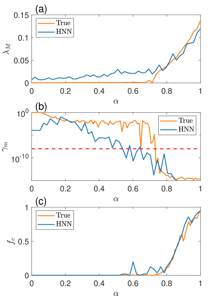
In our calculation, we take 100 equally spaced values of the bifurcation parameter in the unit interval: $\alpha \in [0,1]$. For each $\alpha$ value, we choose 200 random initial conditions and calculate, for each initial condition, the values of the largest Lyapunov exponent and the minimum alignment index. A trajectory is deemed chaotic Zotos (2015) if the largest exponent is positive and the minimum alignment index is less than ${10}^{-8}$. We denote the maximum Lyapunov exponent and the minimum alignment index from the ensemble of 200 trajectories as ${\lambda }_M$ and ${\gamma }_m$, respectively, which are functions of $\alpha$. Another quantity of interest is the fraction of chaotic trajectories, denoted as $f_c$, which also depends on $\alpha$. The triplet of characterizing quantities, ${\lambda }_M$, ${\gamma }_m$, and $f_c$, can be calculated from the HNN and from the original Hamiltonian as a function of $\alpha$. A comparison can then be made to assess the adaptable power of prediction of our parameter-cognizant HNN.

Figures 6(a-c) show the machine predicted and true values of ${\lambda }_M$, ${\gamma }_m$, and $f_c$ versus $\alpha$, respectively, for particle energy $E=1/6$. It can be seen that chaos arises for $\alpha \gtrsim 0.7$, at which ${\lambda }_M$ becomes positive, ${\gamma }_m$ decreases to ${10}^{-8}$, and $f_c$ begins to increase from zero. In Fig. 6(a), the true value of ${\lambda }_M$ for is essentially zero, but the HNN predicted ${\lambda }_M$ is slightly positive. The remarkable feature is that both types of ${\lambda }_M$ value begins to increase appreciably for $\alpha >0.7$. In fact, there is a reasonable agreement between the true and predicted behavior of ${\lambda }_M$. Similar features are present in the behaviors of ${\gamma }_m$ and $f_c$ versus $\alpha$, as shown in Figs. 6(b) and 6(c), respectively. These results are strong evidence that our parameter-cognizant HNN is capable of adaptable prediction of distinct dynamical behaviors in Hamiltonian systems.

IV Issues pertinent to adaptability of Hamiltonian neural networks

We address the adaptability of HNNs by asking the following three questions. First, can the adaptability of HNNs be enhanced by increasing the number of training values of the bifurcation parameter? Second, can adaptability be achieved with multiple parameter channels? Third, does adaptability hold for different target Hamiltonian systems?

IV.1 Effect of number of training parameter values

Figure 7: Effect of increasing the number $N$ of training parameter values on the adaptable prediction error. Shown are the ensemble errors $⟨\mathrm{\Delta }V⟩$ in predicting the potential function for the three simulation settings explained in the text. Increasing $N$ beyond four does not lead to a significant reduction in the errors, indicating that the HNN has already acquired the needed adaptability with training at four different values of the bifurcation parameter.

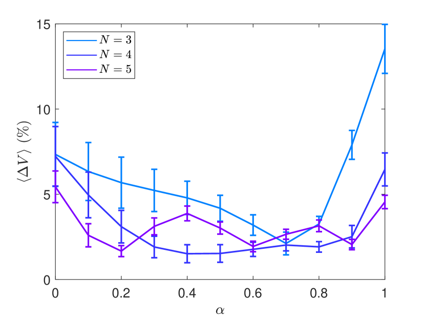
So far, we have used four distinct values of the bifurcation parameter to train our parameter-cognizant HNN. We now investigate if the adaptability can be enhanced by increasing the number of training parameter values. Here by “enhancement” we mean a reduction in the overall errors of predicting the Hamiltonian in a parameter interval that contains values not in the training set. To test this, we conduct the following numerical experiment. We choose $N\ge 3$ training parameter values and, for each parameter value, we train the HNN $M$ times using an ensemble of time series collected from $M$ energy values below the threshold (10 time series from 10 random initial conditions with energy below the threshold). To make the comparison meaningful, we choose the values of $M$ and $N$ such that $NM$ is approximately constant. In particular, for Simulation $\mathrm{\#}$1, we set $N=3$: $\alpha =0.25$, 0.5 and 0.75, and $M=9$. For Simulation $\mathrm{\#}$2, we choose $N=4$: $\alpha =0.2$, 0.4, 0.6, and 0.8, and $M=7$. For Simulation $\mathrm{\#}$3, we have $N=5$: $\alpha =0.1$, 0.3, 0.5, 0.7, and 0.9, and $M=5$. For each simulation, we calculate the ensemble error $⟨\mathrm{\Delta }V⟩$ in predicting the potential function as defined in Eq. (4) for $0\le \alpha \le 1$. The results are shown in Fig. 7. It can be seen that the errors for $N=3$ are generally larger than those for $N>3$, but the errors for the two cases ($N=4$ and 5) are approximately the same, indicating that increasing $N$ above four will not lead to a significant reduction in the errors of adaptable prediction. That is, by training with multiple time series from four values of the bifurcation parameter, the HNN has already acquired the necessary adaptability for predicting the system behavior at other nearby parameter values.

IV.2 HNNs with two parameter channels

Figure 8: Prediction performance of an HNN with two input parameter channels. The target Hamiltonian system is given by the asymmetric Hénon-Heiles system as defined by Eq. (7). Shown is the color-coded ensemble prediction error $⟨\mathrm{\Delta }V⟩$ in the $({\alpha }_1,{\alpha }_2)$ plane. Training is conducted at the 16 points indicated by the green pentagons. The prediction error is small () in the central region $({\alpha }_1,{\alpha }_2)\in [0.2,0.8]$.

We construct parameter-cognizant HNNs with more than one parameter channel. For this purpose, we modify the Hénon-Heiles Hamiltonian Eq. (3) to

$$H=\frac{1}{2}\left(p_1^2+p_2^2\right)+\frac{1}{2}\left(q_1^2+q_2^2\right)+{\alpha }_1{q}_1^2{q}_2-\frac{{\alpha }_2}{3}{q}_2^3,$$ (7)

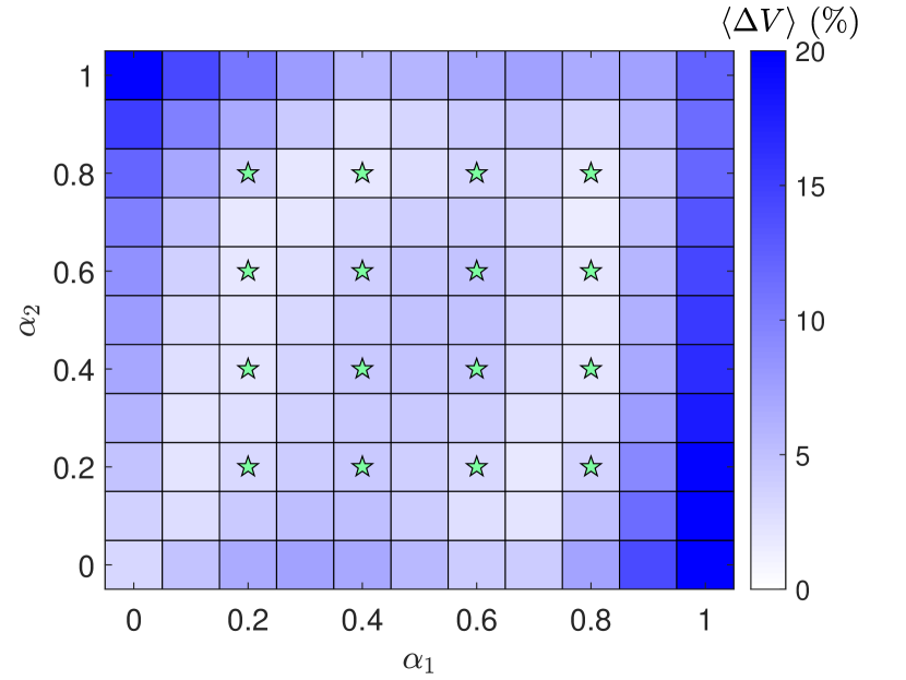
where ${\alpha }_1$ and ${\alpha }_2$ are two independent bifurcation parameters, requiring two independent parameter input channels to the HNN. The energy threshold for bounded motions can be evaluated numerically. We conduct training for a number of combinations of ${\alpha }_1$ and ${\alpha }_2$ values: ${\alpha }_1,{\alpha }_2\in \{0.2,0.4,0.6,0.8\}$. The training data are generated as follows: for each parameter pair, we choose five energy values below the threshold and, for each energy value, a single time series is collected. After the training is done, we predict the potential function for ${\alpha }_1,{\alpha }_2\in [0,1]$ with the interval $0.1$ in each direction of parameter variation. Figure 8 shows the color-coded ensemble prediction error $⟨\mathrm{\Delta }V⟩$ in the $({\alpha }_1,{\alpha }_2)$ plane. For some combinations of ${\alpha }_1$ and ${\alpha }_2$ with a relatively large difference in their values, the threshold energy is less than $1/6$. For such cases, the integration domain in Eq. (4) is modified accordingly based on the threshold value. It can be seen that, in the parameter region $({\alpha }_1,{\alpha }_2)\in (0.2,0.8)$, the prediction error is about $5\%$, while the errors outside the region tend to increase. At the two off-diagonal corners, the errors are the largest, due to the strong asymmetry in the potential profile. Figure 8 demonstrates that HNNs with two parameter channels can be trained to be adaptable for prediction.

IV.3 HNNs for a diatomic molecule system

Figure 9: Parameter-cognizant HNN trained for the one-dimensional Morse system. (a) Shown are the predicted potential profiles for $a=1.0$, 1.5, and 2.0 (solid curves), together with the corresponding true profiles (dashed curves). The predicted potential function for $a=1.5$ is not the interpolation of those for $a=1.0$ and $a=2.0$, attesting to the adaptable predictive power of the HNN. (b) True and predicted orbits in phase space from $[x,p_x]=[1,1]$.

We consider a different target Hamiltonian system, a system defined by the one-dimensional Morse potential that describes the interaction between diatomic molecule Morse (1929). This system was previously used in the study of chaotic scattering Lai (1999); Lai et al. (2000). The Hamiltonian is given by

$$H=\frac{p_x^2}{2}+V(x)\equiv \frac{p_x^2}{2}+{[1-\exp (-a(x-x_0))]}^2-1,$$ (8)

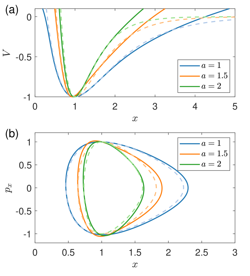
where the potential function $V(x)$ has a minimum value at $x=x_0$ with $V(x_0)=-1$ and $V(x\to \mathrm{\infty })\to 0$. Taking the minimum potential value as the reference point for energy $E$, all orbits are bounded for . We set $x_0=1$ and choose $a$ as the bifurcation parameter. The training data are generated from four different values of $a$: $a=0.5$, 1.0, 2.0, and 4.0 where, for each training parameter value, an ensemble of five values of energy is used, resulting an ensemble of 20 independent time series. The time span for each time series is $0\le t\le 100$ with the sampling time step $\mathrm{\Delta }t=0.1$.

Figure 9 shows the predicted potential profile for $a=1.5$, together with those for the two training points $a=1$ and $a=2$. The result is accurate for $x$ around the minimum potential point, but large errors arise when the position is far away from the minimum point. A plausible reason is that, for large values of $x$, the potential varies slowly, resulting in small changes in the momentum. As a result, the corresponding portions of the time series exhibit less variation, leading to large prediction errors by the HNN. The trained HNN has apparently gained certain adaptability, as the prediction result for $a=1.5$ is not the interpolation of those for $a=1.0$ and $a=2.0$.

V Discussion

Developing adaptable machine learning in general has broad applications to critical problems of current interest. For example, a problem of paramount importance is to predict how a system may behave in the future when some key parameters of the system may have drifted, based on information that is available at the present. As an example, suppose an ecosystem is currently in a normal state. Due to the environmental deterioration, some of its parameters such as the carrying capacity and/or the species decay rates will have drifted in the future. Is it possible to predict if the system will collapse when certain amount of parameter drift has occurred, when the system equations are not known and the only available information is time series data that can be measured prior to but including the present? Adaptable machine learning offers a possible solution. For example, it has been demonstrated recently Kong et al. (2021) that incorporating a parameter-cognizant mechanism into reservoir computing machines enables prediction of possible critical transition and system collapse in the future for any given amount of parameter drift. However, the state-of-the-art reservoir computing schemes under intensive current research Haynes et al. (2015); Larger et al. (2017); Pathak et al. (2017); Lu et al. (2017); Duriez et al. (2017); Lu et al. (2018); Pathak et al. (2018a, b); Carroll (2018); Nakai and Saiki (2018); Roland and Parlitz (2018); Weng et al. (2019); Griffith et al. (2019); Jiang and Lai (2019); Vlachas et al. (2019); Fan et al. (2020); Zhang et al. (2020) do not taken into account physical constraints such as energy conservation, so they are suitable but for dissipative dynamical systems.

Combining the laws of physics and traditional machine learning has the potential to significantly enhance the performance and predictive power of neural networks. It has been demonstrated recently that enforcing the Hamilton’s equations of motion in the traditional feed-forward neural networks can lead to improvement in the prediction accuracy for Hamiltonian systems in both integrable and chaotic regimes Greydanus et al. (2019); Toth et al. (2019); Bertalan et al. (2019); Choudhary et al. (2020a); Garg and Kagi (2019). In these studies, training and prediction are conducted for the same set of parameter values of the target Hamiltonian system, so the underlying Hamiltonian neural networks are not adaptable in the sense that they are not capable of predicting the dynamical behavior of the system at a different parameter setting.

Do adaptable HNNs that we have developed have any practical significance? From the point of view of making predictions of the future states of Hamiltonian systems subject to parameter drifting, the answer is perhaps no. The main reason is that HNNs require all coordinate and momentum time series. For example, one may be interested in predicting whether a complicated many-body astrophysical system may lose its stability and become mostly chaotic in the future, where the only available information is the position and momentum measurements prior to or at the present when the system is still in a mostly integrable regime. As the laws of physics for this system are known, the data required for training is not a lesser burden than knowing the Hamiltonian itself. Nonetheless, our work generates insights into the working of HNNs, as follows.

Our parameter-cognizant, adaptable HNNs have a parameter input channel to the standard multilayer network with the loss function stipulated by the Hamilton’s equations of motion, and are capable of successful prediction of transition to chaos in Hamiltonian systems. In particular, through training with coordinate and momentum time series from four different values of the bifurcation (nonlinearity) parameter, the machine gains adaptability as evidenced by its successful prediction of the dynamical behavior of the target system in an entire parameter interval containing the training parameter values. That is, the benefits of training are that the HNN has learned not only the dynamical “climate” of the target Hamiltonian system but also how the “climate” changes with the bifurcation parameter. Machine learning can thus be viewed as a process by which the neural network self-adjusts its dynamical evolution rules to incorporate those of the target system.

When systematically varying values of the bifurcation parameter are fed into the HNN, it can predict the transition to chaos from a mostly integrable regime, as determined by the ensemble maximum Lyapunov exponent and minimum alignment index as well as the fraction of chaos as a function of the bifurcation parameter. For a single parameter channel, the adaptable predictive power is achieved insofar as the training parameter set contains at least three or four distinct values. For an HNN with duplex parameter channels, the size of the required training parameter set should be at least four by four. Adaptable prediction has also been accomplished for a different Hamiltonian system defined by the Morse potential function. We expect the principle of designing parameter-cognizant HNNs and the training method devised in this paper to hold for general Hamiltonian systems.

One issue is the dependence of the energy surface on the bifurcation parameter. As the parameter changes continuously, the energy surface will evolve accordingly. If we intend to predict the system dynamics for some specific value of the bifurcation parameter for a fixed energy value, the training data sets should contain time series collected from a larger energy value to cover the pertinent phase space region at the desired energy value.

It should also be noted that, using HNNs to predict the transition from integrable dynamics to chaos in the Hénon-Heiles system was first reported Choudhary et al. (2020a), which relied on using energy $E$ as the control parameter for a fixed value of the nonlinearity parameter (e.g., $\alpha =1$). Here we have studied the transition using $\alpha$ as the bifurcation parameter for a fixed energy value (e.g., $E=1/6$). The two routes are equivalent because the Hénon-Heiles system Eq. (3) possesses a three-fold symmetry in the configuration space. Such an equivalence also arises in systems whose potential function contains nonlinear square terms, e.g., the classical ${\varphi }^4$ or FPU model Fermi et al. (1955); Caiani et al. (1998). However, for the two-parameters Hamiltonian Eq. (7) studied in this paper, the three-fold symmetry is broken, destroying the equivalence between varying the nonlinearity parameter and energy. In fact, for Hamiltonian systems such as the Morse and double-pendulum systems, the equivalence does not hold either Morse (1929); Lai et al. (2000); Levien and Tan (1993). Our adaptable HNN does not rely on any such equivalence, and can be effective in predicting the transition to chaos in any type of Hamiltonian systems.

Appendix A Algorithm for calculating the Lyapunov exponent and alignment index of Hamiltonian neural networks

Given a dynamical system $d𝐱/dt=𝐟(𝐱)$, the Jacobi matrix is given by $𝒥=\partial 𝐟/\partial 𝐱$. For a Hamiltonian system, the dynamical variables are $𝐱\equiv {[𝐪,𝐩]}^T$ and

$$𝐟(𝐪,𝐩)=[\frac{\partial H}{\partial 𝐩},-\frac{\partial H}{\partial 𝐪}].$$ (9)

For an HNN, in principle, the Hamiltonian $H$ is given by a sequence of operations of the neural network with the weights and biases in Eq. (1) determined by training. An alternative but efficient approach to calculating the Jacobian matrix $𝒥$ is the finite-difference method. In particular, for a given initial condition, we generate an orbit of $N$ points with time interval $dt$ and calculate $𝒥$ at each time step. Let the sequence of Jacobian matrices be denoted as $𝒥(t_0),𝒥(t_1),\mathrm{\cdots },𝒥(t_N)$, and let $𝒴(t_0)$ be the identity matrix $ℐ$. If the phase space of the target Hamiltonian system is $D$-dimensional ($D=4$ for the Hénon-Heiles system), there are $D$ Lyapunov exponents. Let $𝝀$ be the vector of the $D$ Lyapunov exponents: $𝝀\equiv {({\lambda }_1,{\lambda }_2,\mathrm{\dots },{\lambda }_D)}^T$ and set the initial values of the exponents to be zero: $𝝀(t_0)={(0,0,\mathrm{\dots },0)}^T$. After $N$ steps, we have

$$𝒴(t_N)=𝒥(t_N)\cdot 𝒴(t_{N-1}).$$ (10)

Carrying out the QR decomposition of the matrix $𝒴(t_N)$ with the resulting matrices denoted as $𝒬$ and $ℛ$, we have

${\lambda }_j(t_N)$ $=$ ${\lambda }_j(t_{N-1})+\log |R_{jj}|,$ (11)

$𝒴(t_N)$ $=$ $𝒬,$ (12)

where $R_{jj}$ is the $j$th diagonal element of the matrix $ℛ$. The Lyapunov exponents are given by

$${\lambda }_j=\underset{N\to \mathrm{\infty }}{lim}\frac{{\lambda }_j(t_N)}{Ndt},j=1,\mathrm{\dots },D.$$ (13)

The maximum Lyapunov exponent is ${\lambda }_M={\text{max}}_j({\lambda }_j)$.

To calculate the alignment index, we introduce a matrix $ℳ$ and set it to be the identity matrix at the initial time: $ℳ(t_0)=ℐ$. Let ${𝐮}_1(t_0)={[1,0,0,0]}^T$ and ${𝐮}_2(t_0)={[0,1,0,0]}^T$ be two linearly independent vectors at the initial time. After $N$ steps, we have

(14)

Normalizing the vectors ${𝐮}_{1,2}(t_N)$ by their respective magnitude to have the unit length, we obtain the minimum alignment index as

$${\gamma }_m=\underset{N\to \mathrm{\infty }}{lim}\text{min}(\Vert {𝐮}_1(t_N)+{𝐮}_2(t_N)\Vert ,\Vert {𝐮}_1(t_N)-{𝐮}_2(t_N)\Vert ).$$ (15)

References

- LeCun et al. (2015) Y. LeCun, Y. Bengio, and G. Hinton, “Deep learning,” Nature 521, 436 (2015).
- Goodfellow et al. (2016) I. Goodfellow, Y. Bengio, and A. Courville, Deep Learning (MIT, Cambridge, MA, 2016).
- Jaeger (2001) H. Jaeger, “The “echo state” approach to analysing and training recurrent neural networks-with an erratum note,” German National Research Center for Information Technology GMD Technical Report 148, 13 (2001).
- Mass et al. (2002) W. Mass, T. Nachtschlaeger, and H. Markram, “Real-time computing without stable states: A new framework for neural computation based on perturbations,” Neur. Comp. 14, 2531 (2002).
- Jaeger and Haas (2004) H. Jaeger and H. Haas, “Harnessing nonlinearity: Predicting chaotic systems and saving energy in wireless communication,” Science 304, 78 (2004).
- Manjunath and Jaeger (2013) G. Manjunath and H. Jaeger, “Echo state property linked to an input: Exploring a fundamental characteristic of recurrent neural networks,” Neur. Comp. 25, 671 (2013).
- Haynes et al. (2015) N. D. Haynes, M. C. Soriano, D. P. Rosin, I. Fischer, and D. J. Gauthier, “Reservoir computing with a single time-delay autonomous Boolean node,” Phys. Rev. E 91, 020801 (2015).
- Larger et al. (2017) L. Larger, A. Baylón-Fuentes, R. Martinenghi, V. S. Udaltsov, Y. K. Chembo, and M. Jacquot, “High-speed photonic reservoir computing using a time-delay-based architecture: Million words per second classification,” Phys. Rev. X 7, 011015 (2017).
- Pathak et al. (2017) J. Pathak, Z. Lu, B. Hunt, M. Girvan, and E. Ott, “Using machine learning to replicate chaotic attractors and calculate Lyapunov exponents from data,” Chaos 27, 121102 (2017).
- Lu et al. (2017) Z. Lu, J. Pathak, B. Hunt, M. Girvan, R. Brockett, and E. Ott, “Reservoir observers: Model-free inference of unmeasured variables in chaotic systems,” Chaos 27, 041102 (2017).
- Duriez et al. (2017) T. Duriez, S. L. Brunton, and B. R. Noack, Machine Learning Control - Taming Nonlinear Dynamics and Turbulence (Springer, 2017).
- Lu et al. (2018) Z. Lu, B. R. Hunt, and E. Ott, “Attractor reconstruction by machine learning,” Chaos 28, 061104 (2018).
- Pathak et al. (2018a) J. Pathak, A. Wilner, R. Fussell, S. Chandra, B. Hunt, M. Girvan, Z. Lu, and E. Ott, “Hybrid forecasting of chaotic processes: Using machine learning in conjunction with a knowledge-based model,” Chaos 28, 041101 (2018a).
- Pathak et al. (2018b) J. Pathak, B. Hunt, M. Girvan, Z. Lu, and E. Ott, “Model-free prediction of large spatiotemporally chaotic systems from data: A reservoir computing approach,” Phys. Rev. Lett. 120, 024102 (2018b).
- Carroll (2018) T. L. Carroll, “Using reservoir computers to distinguish chaotic signals,” Phys. Rev. E 98, 052209 (2018).
- Nakai and Saiki (2018) K. Nakai and Y. Saiki, “Machine-learning inference of fluid variables from data using reservoir computing,” Phys. Rev. E 98, 023111 (2018).
- Roland and Parlitz (2018) Z. S. Roland and U. Parlitz, “Observing spatio-temporal dynamics of excitable media using reservoir computing,” Chaos 28, 043118 (2018).
- Weng et al. (2019) T. Weng, H. Yang, C. Gu, J. Zhang, and M. Small, “Synchronization of chaotic systems and their machine-learning models,” Phys. Rev. E 99, 042203 (2019).
- Griffith et al. (2019) A. Griffith, A. Pomerance, and D. J. Gauthier, “Forecasting chaotic systems with very low connectivity reservoir computers,” Chaos 29, 123108 (2019).
- Jiang and Lai (2019) J. Jiang and Y.-C. Lai, “Model-free prediction of spatiotemporal dynamical systems with recurrent neural networks: Role of network spectral radius,” Phys. Rev. Research 1, 033056 (2019).
- Vlachas et al. (2019) P. R. Vlachas, J. Pathak, B. R. Hunt, T. P. Sapsis, M. Girvan, E. Ott, and P. Koumoutsakos, “Forecasting of spatio-temporal chaotic dynamics with recurrent neural networks: A comparative study of reservoir computing and backpropagation algorithms,” arXiv preprint arXiv:1910.05266 (2019).
- Fan et al. (2020) H. Fan, J. Jiang, C. Zhang, X. Wang, and Y.-C. Lai, “Long-term prediction of chaotic systems with machine learning,” Phys. Rev. Research 2, 012080 (2020).
- Zhang et al. (2020) C. Zhang, J. Jiang, S.-X. Qu, and Y.-C. Lai, “Predicting phase and sensing phase coherence in chaotic systems with machine learning,” Chaos 30, 083114 (2020).
- De Wilde (1993) P. De Wilde, “Class of Hamiltonian neural networks,” Phys. Rev. E 47, 1392 (1993).
- Greydanus et al. (2019) S. Greydanus, M. Dzamba, and J. Yosinski, “Hamiltonian neural networks,” arXiv:1906.01563 (2019).
- Toth et al. (2019) P. Toth, D. J. Rezende, A. Jaegle, S. Racanière, A. Botev, and I. Higgins, “Hamiltonian generative networks,” arXiv:1909.13789 (2019).
- Bertalan et al. (2019) T. Bertalan, F. Dietrich, I. Mezić, and I. G. Kevrekidis, “On learning Hamiltonian systems from data,” Chaos 29, 121107 (2019).
- Choudhary et al. (2020a) A. Choudhary, J. F. Lindner, E. G. Holliday, S. T. Miller, S. Sinha, and W. L. Ditto, “Physics-enhanced neural networks learn order and chaos,” Phys. Rev. E 101, 062207 (2020a).
- Garg and Kagi (2019) A. Garg and S. S. Kagi, “Hamiltonian neural networks,” https://github.com/ayushgarg31/HNN-Neurips2019 (2019).
- Chen et al. (2019) Z. Chen, J. Zhang, M. Arjovsky, and L. Bottou, “Symplectic recurrent neural networks,” arXiv:1909.13334 (2019).
- Cranmer et al. (2020) M. Cranmer, S. Greydanus, S. Hoyer, P. Battaglia, D. Spergel, and S. Ho, “Lagrangian neural networks,” arXiv preprint arXiv:2003.04630 (2020).
- Sanchez-Gonzalez et al. (2019) A. Sanchez-Gonzalez, V. Bapst, K. Cranmer, and P. Battaglia, “Hamiltonian graph networks with ode integrators,” arXiv preprint arXiv:1909.12790 (2019).
- Dulberg and Cohen (2020) Z. Dulberg and J. Cohen, “Learning canonical transformations,” arXiv preprint arXiv:2011.08822 (2020).
- Choudhary et al. (2020b) A. Choudhary, J. F. Lindner, E. G. Holliday, S. T. Miller, S. Sinha, and W. L. Ditto, “Forecasting Hamiltonian dynamics without canonical coordinates,” arXiv preprint arXiv:2010.15201 (2020b).
- Lutter et al. (2019) M. Lutter, C. Ritter, and J. Peters, “Deep Lagrangian networks: Using physics as model prior for deep learning,” arXiv preprint arXiv:1907.04490 (2019).
- Havoutis and Ramamoorthy (2010) I. Havoutis and S. Ramamoorthy, “Geodesic trajectory generation on learnt skill manifolds,” in 2010 IEEE International Conference on Robotics and Automation (IEEE, 2010) pp. 2946–2952.
- Falahian et al. (2015) R. Falahian, M. M. Dastjerdi, M. Molaie, S. Jafari, and S. Gharibzadeh, “Artificial neural network-based modeling of brain response to flicker light,” Nonlinear Dyn. 81, 1951 (2015).
- Cestnik and Abel (2019) R. Cestnik and M. Abel, “Inferring the dynamics of oscillatory systems using recurrent neural networks,” Chaos 29, 063128 (2019).
- Kim et al. (2020) J. Z. Kim, Z. Lu, E. Nozari, G. J. Pappas, and D. S. Bassett, “Teaching recurrent neural networks to modify chaotic memories by example,” arXiv preprint arXiv:2005.01186 (2020).
- Klos et al. (2020) C. Klos, Y. F. K. Kossio, S. Goedeke, A. Gilra, and R.-M. Memmesheimer, “Dynamical learning of dynamics,” Phys. Rev. Lett. 125, 088103 (2020).
- Kong et al. (2021) L.-W. Kong, H.-W. Fan, C. Grebogi, and Y.-C. Lai, “Machine learning prediction of critical transition and system collapse,” Phys. Rev. Research 3, 013090 (2021).
- Guest et al. (2018) D. Guest, K. Cranmer, and D. Whiteson, “Deep learning and its application to LHC physics,” Annu. Rev. Nucl. Part. Sci. 68, 161 (2018).
- Radovic et al. (2018) A. Radovic, M. Williams, D. Rousseau, M. Kagan, D. Bonacorsi, A. Himmel, A. Aurisano, K. Terao, and T. Wongjirad, “Machine learning at the energy and intensity frontiers of particle physics,” Nature 560, 41 (2018).
- Carleo and Troyer (2017) G. Carleo and M. Troyer, “Solving the quantum many-body problem with artificial neural networks,” Science 355, 602 (2017).
- Peurifoy et al. (2018) J. Peurifoy, Y. Shen, L. Jing, Y. Yang, F. Cano-Renteria, B. G. DeLacy, J. D. Joannopoulos, M. Tegmark, and M. Soljačić, “Nanophotonic particle simulation and inverse design using artificial neural networks,” Sci. Adv. 4, eaar4206 (2018).
- Dunjko and Briegel (2018) V. Dunjko and H. J. Briegel, “Machine learning & artificial intelligence in the quantum domain: a review of recent progress,” Rep. Prog. Phys. 81, 074001 (2018).
- Carleo et al. (2019) G. Carleo, I. Cirac, K. Cranmer, L. Daudet, M. Schuld, N. Tishby, L. Vogt-Maranto, and L. Zdeborová, “Machine learning and the physical sciences,” Rev. Mod. Phys. 91, 045002 (2019).
- Iten et al. (2020) R. Iten, T. Metger, H. Wilming, L. Del Rio, and R. Renner, “Discovering physical concepts with neural networks,” Phys. Rev. Lett. 124, 010508 (2020).
- Karkar et al. (2020) S. Karkar, I. Ayed, E. de Bézenac, and P. Gallinari, “A principle of least action for the training of neural networks,” arXiv preprint arXiv:2009.08372 (2020).
- Yang et al. (2020) S. Yang, X. He, and B. Zhu, “Learning physical constraints with neural projections,” Adv. Neu. Info. Process. Sys. 33 (2020).
- Abadi et al. (2016) M. Abadi, P. Barham, J. Chen, Z. Chen, A. Davis, J. Dean, M. Devin, S. Ghemawat, G. Irving, M. Isard, et al., “Tensorflow: A system for large-scale machine learning,” in 12th USENIX symposium on operating systems design and implementation (OSDI 16) (2016) pp. 265–283.
- Chollet et al. (2015) F. Chollet et al., “Keras,” https://keras.io (2015).
- Hénon and Heiles (1964) M. Hénon and C. Heiles, “The applicability of the third integral of motion: some numerical experiments,” Astron. J. 69, 73 (1964).
- Waite and Miller (1981) B. A. Waite and W. H. Miller, “Mode specificity in unimolecular reaction dynamics: The Henon–Heiles potential energy surface,” J. Chem. Phys. 74, 3910 (1981).
- Feit and Fleck Jr (1984) M. Feit and J. Fleck Jr, “Wave packet dynamics and chaos in the Hénon–Heiles system,” J. Chem. Phys. 80, 2578 (1984).
- Vendrell and Meyer (2011) O. Vendrell and H.-D. Meyer, “Multilayer multiconfiguration time-dependent Hartree method: Implementation and applications to a Henon–Heiles Hamiltonian and to pyrazine,” J. Chem. Phys. 134, 044135 (2011).
- de Moura and Letelier (1999) A. P. de Moura and P. S. Letelier, “Fractal basins in Hénon–Heiles and other polynomial potentials,” Phys. Lett. A 256, 362 (1999).
- Seoane et al. (2006) J. M. Seoane, J. Aguirre, M. A. Sanjuán, and Y.-C. Lai, “Basin topology in dissipative chaotic scattering,” Chaos 16, 023101 (2006).
- Seoane et al. (2007) J. M. Seoane, M. A. Sanjuán, and Y.-C. Lai, “Fractal dimension in dissipative chaotic scattering,” Phys. Rev. E 76, 016208 (2007).
- Lichtenberg and Lieberman (1992) A. Lichtenberg and M. Lieberman, Regular and Chaotic Dynamics, 2nd ed. (Springer, Berlin, New York, 1992).
- Skokos (2001) C. Skokos, “Alignment indices: a new, simple method for determining the ordered or chaotic nature of orbits,” J. Phys. A Math. Gen. 34, 10029 (2001).
- Zotos (2015) E. E. Zotos, “Classifying orbits in the classical Hénon–Heiles Hamiltonian system,” Nonlinear Dyn. 79, 1665 (2015).
- Morse (1929) P. M. Morse, “Diatomic molecules according to the wave mechanics II. Vibrational levels,” Phys. Rev. 34, 57 (1929).
- Lai (1999) Y.-C. Lai, “Abrupt bifurcation to chaotic scattering with discontinuous change in fractal dimension,” Phys. Rev. E 60, R6283 (1999).
- Lai et al. (2000) Y.-C. Lai, A. P. De Moura, and C. Grebogi, “Topology of high-dimensional chaotic scattering,” Phys. Rev. E 62, 6421 (2000).
- Fermi et al. (1955) E. Fermi, P. Pasta, S. Ulam, and M. Tsingou, Studies of the nonlinear problems, Tech. Rep. (Los Alamos National Laboratory, 1955).
- Caiani et al. (1998) L. Caiani, L. Casetti, C. Clementi, G. Pettini, M. Pettini, and R. Gatto, “Geometry of dynamics and phase transitions in classical lattice -4 theories,” Phys. Rev. E 57, 3886 (1998).
- Levien and Tan (1993) R. B. Levien and S. M. Tan, “Double pendulum: An experiment in chaos,” Am. J. Phys. 61, 1038 (1993).