Heterogeneity for the Win: One-Shot Federated Clustering

Abstract

In this work, we explore the unique challenges—and opportunities—of unsupervised federated learning (FL). We develop and analyze a one-shot federated clustering scheme, k-FED, based on the widely-used Lloyd’s method for $k$-means clustering. In contrast to many supervised problems, we show that the issue of statistical heterogeneity in federated networks can in fact benefit our analysis. We analyse k-FED under a center separation assumption and compare it to the best known requirements of its centralized counterpart. Our analysis shows that in heterogeneous regimes where the number of clusters per device $(k^{\prime })$ is smaller than the total number of clusters over the network $k$, $(k^{\prime }\le \sqrt{k})$, we can use heterogeneity to our advantage—significantly weakening the cluster separation requirements for k-FED. From a practical viewpoint, k-FED also has many desirable properties: it requires only one round of communication, can run asynchronously, and can handle partial participation or node/network failures. We motivate our analysis with experiments on common FL benchmarks, and highlight the practical utility of one-shot clustering through use-cases in personalized FL and device sampling.

1 Introduction

Federated learning (FL) aims to perform machine learning over large, heterogeneous networks of devices such as mobile phones or wearables (McMahan et al., 2017). While significant attention has been given to the problem of supervised learning in such settings, the problem of unsupervised federated learning has been relatively unexplored (Kairouz et al., 2019). In this work, we show that unsupervised learning presents unique opportunities for FL, specifically for the task of clustering data that resides in a federated network.

Clustering is a crucial first step in many learning tasks. In the case of federated learning, clustering has found applications in client-selection (Cho et al., 2020), personalization (Ghosh et al., 2020) and exploratory data analysis. While many works have explored techniques for distributed clustering (Section 2), most do not take into account the unique challenges of federated learning, such as statistical heterogeneity, systems heterogeneity, and stringent communication constraints (Li et al., 2020a). These challenges can complicate analyses, reduce efficiency, and lead to practical issues with stragglers and device failures. In this work, we study communication-efficient distributed clustering in settings where the data is non-identically distributed across the network (i.e., heterogeneous), and devices can join and leave the network abruptly. For such settings, we develop and analyse a one-shot clustering scheme, k-FED, based on the classical Lloyd’s heuristic (Lloyd, 1982) for clustering.

The method we propose, k-FED, requires only one round of communication with a central server. Each device, indexed by $z$, solves a local $k^{(z)}$-means problem and then communicates its local cluster means via a message of size $O(d{k}^{(z)})$. As we show in Section 3, this allows for device failures, only requiring that there are enough devices available in the network such that $k$ target clusters exist in the data. Moreover, it is possible to cluster points in previously unavailable devices via a simple recomputation at the central server.

Beyond the practical benefits of k-FED, our work is unique in rigorously demonstrating a problem setting where possible benefits of statistical heterogeneity exist for federated learning. In particular, in supervised learning, many works have highlighted detrimental effects of statistical heterogeneity, observing that heterogeneity can lead to poor convergence for federated optimization methods (McMahan et al., 2017; Li et al., 2020b), result in unfair models (Mohri et al., 2019), or necessitate novel forms of personalization (Smith et al., 2017; Mansour et al., 2020). In contrast to these works, we show that for the specific notion of heterogeneity considered herein (provided in Definition 3.2 and motivated by the application of clustering), heterogeneity can in fact have measurable benefits for our approach.

More specifically, similar to many works in clustering (Kumar & Kannan (2010); Awasthi & Sheffet (2012) and references therein), we analyse k-FED under a center-separation assumption; that is, we assume that the mean of the clusters are well separated. We also consider a specific notion of heterogeneity: given a target clustering with $k$ clusters that we wish to recover from the data, we assume that each device contains data from only $k^{\prime }\le \sqrt{k}$ of these target clusters. For instance, for clustering data generated by a mixture of $k$ well separated Gaussians, we assume that each device contains data from $k^{\prime }\le \sqrt{k}$ component Gaussians. In this regime, we show that our separation requirement is similar to that of the centralized counterpart. Further, while the centralized setting requires all pairs of cluster centers to satisfy a $\mathrm{\Omega }(\sqrt{k})$ center separation requirement, the federated approach can handle a large fraction of cluster pairs only satisfying a weaker $\mathrm{\Omega }(k^{\frac{1}{4}})$ separation requirement. This is the first result we are aware of that analyzes the benefits of heterogeneity in the context of federated clustering.

Contributions. We propose and analyze a one-shot communication scheme for federated clustering. Our proposed method, k-FED, addresses common practical concerns in federated settings, such as high communication costs, stragglers, and device failures. Theoretically, we show that k-FED performs similarly to centralized clustering in regimes where each device only has data from at most $\sqrt{k}$ clusters with a similar $\mathrm{\Omega }(\sqrt{k})$ center separation requirement. Moreover, in contrast to the centralized setting, we show that a large number of cluster pairs need only a $\mathrm{\Omega }(k^{\frac{1}{4}})$ weaker separation assumption in heterogeneous networks, thus allowing a broader class of problems to be solved in this setting compared with centralized clustering. We demonstrate our method through experiments on common FL benchmarks, and explore the applicability of k-FED to problems in personalized federated learning and device sampling. Our work highlights that heterogeneity can have distinct benefits for a subset of problems in federated learning.

2 Background and Related Work

Centralized Clustering. Clustering is one of the most widely-used unsupervised learning tasks, and has been extensively studied in both centralized and distributed settings. Although a variety of clustering methods exist, Lloyd’s heuristic (Lloyd, 1982) remains popular due in part to its simplicity. In Lloyd’s method, we start with an initial set of $k$ centers. We then assign each point to its nearest center and reassign the centers to be the mean of all the points assigned to it, continuing this process till termination. While it is easy to show that this method terminates, it is also known that this process can take superpolynomial time to converge (Arthur & Vassilvitskii, 2006). However, under suitable assumptions and careful choice of the initial centers, it can be shown to converge in polynomial time (Arthur & Vassilvitskii, 2006; Ostrovsky et al., 2013; Kumar & Kannan, 2010; Awasthi & Sheffet, 2012).

The method we propose, k-FED (Section 3.2), is a simple, communication-efficient distributed variant of these classical techniques. k-FED runs a variant of Lloyd’s method for $k$-means clustering locally on each device, and then performs one round of communication to aggregate and assign clusters. Our work builds on the analysis of a variant of Lloyd’s algorithm developed by Kumar & Kannan (2010) and later improved in Awasthi & Sheffet (2012) for the problem of clustering data from mixture distributions and other related results (e.g., McSherry, 2001; Ostrovsky et al., 2013). These works develop a deterministic framework with no generative assumptions on the data. Our analysis follows this framework and does not make any generative assumptions on the data.

Parallel and Distributed Clustering. Many works have explored parallel or distributed implementations of centralized clustering techniques (Dhillon & Modha, 2002; Tasoulis & Vrahatis, 2004; Datta et al., 2005; Bahmani et al., 2012; Xu et al., 1999). Unlike the one-shot communication scheme explored herein, these methods are typically direct parallel implementations of methods such as Lloyd’s heuristic or DBSCAN (Ester et al., 1996), and require numerous rounds of communication. Another line of work has considered communication-efficient distributed clustering variants that require only one or two rounds of communication (e.g., Kargupta et al., 2001; Januzaj et al., 2004; Feldman et al., 2012; Balcan et al., 2013; Bateni et al., 2014; Bachem et al., 2018). These works are mostly empirical, in that there are no provable guarantees on the approximation quality of the distributed schemes; the works of Balcan et al. (2013); Bateni et al. (2014); Bachem et al. (2018) differ by providing communication-efficient distributed coreset methods for clustering, along with provable approximation guarantees. However, these works do not explore the federated setting or potential benefits of heterogeneity.

Federated Clustering. Several works have explored clustering in the context of supervised FL as a way to better model non-IID data (Smith et al., 2017; Ghosh et al., 2019, 2020; Sattler et al., 2020). These works differ from our own by clustering specifically in terms of devices, focusing on the downstream supervised learning task, and using either iterative (Smith et al., 2017; Ghosh et al., 2020; Sattler et al., 2020) or centralized (Ghosh et al., 2019) clustering schemes. Though not the main of focus of our work, in Section 4 we demonstrate the applicability of one-shot clustering by showing how k-FED can be used as a simple pre-processing step to deliver personalized federated learning—achieving similar or superior performance relative to the recent iterative approach for clustered FL proposed in Ghosh et al. (2020).

More recently, a distributed matrix factorization based clustering approach was explored in Wang & Chang (2020) for the purposes of unsupervised learning. However, while the authors consider the impact of statistical heterogeneity on their convergence guarantees, the focus is not on one-shot clustering or on showing distinct benefits of heterogeneity in their analyses.

3 k-FED: Preliminaries and Main Results

In this section, we begin by discussing some preliminaries and existing results in clustering related to Lloyd-type methods. In Section 3.1, we present the deterministic framework of Awasthi & Sheffet (2012) for centralized clustering, which we build upon. We present our method k-FED and state our theoretical results in Section 3.2. We provide detailed proofs in Appendix A.

3.1 Centralized $k$-means

In the standard (centralized) $k$-means problem, we are given a matrix $A\in {ℝ}^{n\times d}$ where each row $A_i$ is a data point in ${ℝ}^d$. We are also given a fixed positive integer $k\le n$, and our objective is to partition the data points into $k$ disjoint partitions, $𝒯=(T_1,\mathrm{\dots },T_k),$ so as to minimize the $k$-means cost:

$$\varphi (𝒯)=\sum _{j=1}^k\sum _{i\in T_j}{\parallel A_i-\mu (T_j)\parallel }_2^2.$$ (1)

Here we use $\mu (S)$ as an operator to indicate the mean of the points indexed by $S$, i.e., $\mu (S)=\frac{1}{|S|}{\sum }_{i\in S}{A}_i$. To ease notation, we simplify this as ${\mu }_r:=\mu (T_r)$, when $T_r$ is unambiguous.

Algorithm 1 Local $k^{(z)}$-means (Awasthi & Sheffet, 2012)

1: Input: On device indexed by $z$, the matrix of data points $A^{(z)}$, integer $k^{(z)}$;

2: Project $A^{(z)}$ onto the subspace spanned by the top $k^{(z)}$ singular vectors to get ${\widehat{A}}^{(z)}$. Run any standard $10$-approximation algorithm on the projected data and estimate $k^{(z)}$ centers (${\nu }_1,{\nu }_2,\mathrm{\dots },{\nu }_{k^{(z)}}$).

3: Set

$$S_r\leftarrow \{i:{\parallel {\widehat{A}}_i^{(z)}-{\nu }_r\parallel }_2\le \frac{1}{3}{\parallel {\widehat{A}}_i^{(z)}-{\nu }_s\parallel }_2,\text{for every}s\}$$

and ${\theta }_r^{(z)}\leftarrow \mu (S_r)$

4: Run Lloyd steps until convergence

$$U_r^{(z)}\leftarrow \{i:{\parallel A_i^{(z)}-{\theta }_r^{(z)}\parallel }_2\le {\parallel A_i^{(z)}-{\theta }_s^{(z)}\parallel }_2,\forall s\}$$

and ${\theta }_r^{(z)}\leftarrow \mu (U_r^{(z)})$.

5: Return: Cluster assignments $(U_1^{(z)},U_2^{(z)},\mathrm{\dots },U_{k^{(z)}}^{(z)})$ and their means ${\mathrm{\Theta }}^{(z)}=({\theta }_1^{(z)},\mathrm{\dots },{\theta }_{k^{(z)}})$.

While the k-means problem as stated here does not specify any generative model for the data points $A_i$, a popular setting to consider is when the data is sampled from a mixture of $k$-distributions in $d$-dimensions ($k\ll d$). For instance, we could imagine the data points as being sampled from a mixture of $k$ Gaussian distributions. This generative model also introduces a notion of a target clustering, $𝒯=(T_1,\mathrm{\dots },T_k)$ where the set $T_i$ contains all points generated by the $i$-th component distribution. Many distribution dependent results are known for the problem of clustering distributions (see Kumar & Kannan (2010)). In general, they can be stated as: If the means of the distributions are $\text{poly}(k)$ standard deviations apart, then we can cluster the data in polynomial time. Kumar & Kannan (2010) introduce a deterministic (distribution independent) framework that encompasses many of these known results. This work was later simplified and improved by Awasthi & Sheffet (2012). We state the main results of this framework here, after stating the notation we use. We emphasis that in our analysis we make no assumptions on how the data is generated; all relevant quantities only depend on the provided data.

Notation. We now introduce several definitions and notations that will be used throughout the paper. Let $\parallel A\parallel$ denote the spectral norm of a matrix $A$, defined as $\parallel A\parallel ={\max }_{u:{\parallel u\parallel }_2=1}{\parallel Au\parallel }_2$, and let ${\parallel A_i\parallel }_2$ denote the ${\mathrm{\ell }}_2$ norm of a vector $A_i$. For consistency, we index individual rows of $A$ with $i$ and $j$. Moreover, when a target clustering $T_1,\mathrm{\dots },T_k$ is fixed, we index clusters with $r,s$, e.g., $A_r$ is the matrix of points indexed by $T_r$. For notational convenience, we let $c(A_i)$ to denote the cluster index for data point $A_i$ such that, $A_i\in T_{c(A_i)}$. For some set of points $M$, and another point say $x$, let $d_M(x)$ denote the distance of $x$ to the set $M$, defined as $d_M(x)={\min }_{y\in M}{\parallel x-y\parallel }_2$. Finally, let $C$ be a $n\times d$ matrix with each row $C_i={\mu }_{c(A_i)}$. For cluster $T_r$ with $n_r=|T_r|$, we define

$${\tilde{\mathrm{\Delta }}}_r:=\sqrt{k}\frac{\parallel A-C\parallel }{\sqrt{n_r}}.$$ (2)

Here the quantity $\parallel A-C\parallel /\sqrt{n_r}$ can be thought of as a deterministic analogue of the standard deviation; it measures the maximum average variance along any direction. Thus instead of reasoning about the separation between two clusters $T_r$ and $T_s$ in terms of the standard deviation, we will use $({\tilde{\mathrm{\Delta }}}_r+{\tilde{\mathrm{\Delta }}}_s)$. In particular, we say that the two clusters $T_r$ and $T_s$ are well separated if for large enough constant $c$, their means satisfy:

${\parallel {\mu }_r-{\mu }_s\parallel }_2\ge c({\tilde{\mathrm{\Delta }}}_r+{\tilde{\mathrm{\Delta }}}_s).$ (3)

Again, we can interpret this as saying that two clusters are well separated if their means are $c$-standard-deviations apart. Using the center separation assumption in (3), Awasthi & Sheffet (2012) show that for a target clustering $T_1,T_2,\mathrm{\dots },T_k$ satisfying the separation assumption, the variant of Lloyd’s algorithm presented in Algorithm-1 when applied to the centralized clustering problem correctly clusters all but a small fraction of the data points. We state their result formally in Lemma 1, but before that we define a proximity condition, that will be used to precisely characterize the misclassified points.

Definition 3.1.

A point $A_i$ for some $i\in T_s$ is said to satisfy the proximity condition, if for every $r\ne s$, the projection of $A_i$ onto the line connecting ${\mu }_r$ and ${\mu }_s$, denoted by ${\overline{A}}_i$ satisfies

$${\parallel {\overline{A}}_i-{\mu }_r\parallel }_2-{\parallel {\overline{A}}_i-{\mu }_s\parallel }_2\ge \left(\frac{1}{\sqrt{n_r}}+\frac{1}{\sqrt{n_s}}\right)\parallel A-C\parallel .$$

Thus a point $A_i$ for $i\in T_s$ satisfies the proximity condition if its projection on the line connecting ${\mu }_r$ and ${\mu }_s$ is closer to ${\mu }_s$ by $\parallel A-C\parallel (\frac{1}{\sqrt{n_r}}+\frac{1}{\sqrt{n_s}})$. We refer to points that do not satisfy the proximity condition as ‘bad points’. We now state the main result from Awasthi & Sheffet (2012) in the following lemma.

Lemma 1 (Awasthi-Sheffet, 2011).

Let $𝒯=(T_1,\mathrm{\dots },T_k)$ be the target clustering. Assume that each pair of clusters $T_r$ and $T_s$ are well separated. Then, after step 2 of Algorithm-1, for every $r$, it holds that ${\parallel \mu (S_r)-{\mu }_r\parallel }_2\le \frac{25}{c}\frac{1}{\sqrt{n_r}}\parallel A-C\parallel$. Moreover, if the number of bad points is $ϵn$, then (a) the clustering $\{U_1,U_2,\mathrm{\dots },U_k\}$ misclassifies no more than $(ϵ+O(1)c^{-4})n$ points and (b) . Finally, if $ϵ=0$ then all points are correctly assigned.

When we say misclassify, we mean with respect to $𝒯$ and up to a permutation of labels. Lemma 1 tells us that the cluster means, $\mu (S_r)$, are not very far away from the target cluster means, ${\mu }_r$. Note that there are no distribution dependent terms in this statement; all relevant quantities are defined in terms of the data matrix $A$ and $𝒯$.

3.2 k-FED: Method and Main Result

We now turn our attention to clustering data in a federated network. In our setting, we assume that all the devices in the network can communicate with a central server. Our clustering method k-FED, described in Algorithm 2, can be thought of as working in two stages. In the first stage, each device solves a local clustering subproblem and computes the cluster means for this subproblem. In the second stage, the central server accumulates and aggregates the results to compute the final clustering.

Notation. Let $A$ be an $n\times d$ data matrix of all the data points in our network. We index individual devices by $z\in [Z]$ and thus, we denote the data-matrix for any particular device by $A^{(z)}\in {ℝ}^{n^{(z)}\times d}$, where $n^{(z)}$ is the number of data points on the device. Let $n_{\min }={\min }_z{n}^{(z)}$. Note that $A^{(z)}$ is some subset of rows of $A$. Let $𝒯=(T_1,\mathrm{\dots },T_k)$ be a clustering of all the data, referred to as a target clustering. For a fixed $𝒯$, let ${𝒯}^{(z)}=(T_1^{(z)},T_2^{(z)},\mathrm{\dots },T_k^{(z)})$ be subsets of our target clustering that reside on a device $z$. Note that some $T_r^{(z)}$ could be empty. Let $k^{(z)}$ be the number of non-empty subsets on device $z$ and let $k^{\prime }={\max }_z{k}^{(z)}$. Our notion of heterogeneity is formally defined based on the value of $k^{\prime }$, as described below.

Definition 3.2 (Heterogeneity of Clustering).

In the context of clustering, we say that a federated network with sufficient data is heterogeneous if $k^{\prime }\le \sqrt{k}$. The lower the ratio between $k^{\prime }$ and $\sqrt{k}$, the more heterogeneity exists in the network.

Intuitively, this definition of heterogeneity states that—in contrast to the data from the $k$ total clusters being partitioned in an IID fashion across the network—the data are partitioned in an non-IID fashion, such that only data from a small number of clusters (at most $k^{\prime }$) exists on each device. Such non-IID partitioning is reasonable to expect in heterogeneous federated networks with a large number of clusters, since the distribution of data on each device may differ, and it is not possible to actively re-distribute data across the network. For instance, consider identifying interests of mobile phone users based on the interaction data on an application. Here the interaction data is generated by the user on their particular device, and will reflect the tastes of individual. While the total number of ‘tastes’ (clusters) over the entire network could be quite large, a typical user will be interested in only a small number of them. With this definition in mind, we next describe our one-shot clustering method, k-FED, and analyze it in heterogeneous regimes.

Method Description.

Similar to the centralized case (Section 3.1), let $C^{(z)}$ be a $n^{(z)}\times d$ matrix of the local cluster means, i.e. of ${𝒯}^{(z)}$. Consider a non-empty susbset $T_r^{(z)}$ of cluster $T_r$ on some device and let $n_r^{(z)}=|T_r^{(z)}|$. We assume that there is a constant $m_0>1$, such that $n_r^{(z)}\ge \frac{1}{m_0}{n}_r$ for all $r$. We will use this quantity to ensure that individual devices have ‘enough’ points. Let,

${\mathrm{\Delta }}_r=k^{\prime }{\displaystyle \frac{\parallel A-C\parallel }{\sqrt{n_r}}},\text{and}\lambda =\sqrt{k^{\prime }}\left({\displaystyle \frac{\parallel A-C\parallel }{\sqrt{n_{\min }}}}\right).$ (4)

In the first step of k-FED (Algorithm-2), each (available) device $z\in [Z]$ runs Algorithm-1 locally and solves a local clustering problem with their local dataset $A^{(z)}$ and parameter $k^{(z)}$. We assume that $k^{(z)}$ is known. This stage outputs device cluster centers ${\mathrm{\Theta }}^{(z)}=({\theta }_1^{(z)},\mathrm{\dots },{\theta }_{k^{(z)}}^{(z)})$ and cluster assignments, $U_1^{(z)},\mathrm{\dots },U_{k^{(z)}}^{(z)}$ for each device $z$. At this stage, note that even though each device has classified its own points into clusters, we do not yet have a clustering for points across devices. The central server attempts to create this clustering by aggregating the device cluster centers and separating them into $k$ sets, ${\tau }_1,\mathrm{\dots },{\tau }_k$. These sets induce a clustering of the data on the network as defined here:

Definition 3.3 (k-FED induced clustering).

Let ${\tau }_1,{\tau }_2,\mathrm{\dots },{\tau }_k$ be the clustering of device centers returned by Algorithm 2. Define,

$$T_r^{\prime }=\{i:A_i^{(z)}\in U_s^{(z)}\text{and}{\theta }_s^{(z)}\in {\tau }_r,z\in [Z],s\in [k^{(z)}]\}.$$

Then, ${𝒯}^{\prime }=(T_1^{\prime },\mathrm{\dots },T_k^{\prime })$ form a disjoint partition of the entire data, called the k-FED induced clustering.

Algorithm 2 k-FED

1: On each device $z\in [Z]$, run Algorithm-1 with local data $A^{(z)}$ and $k^{(z)}$ and obtain device cluster centers ${\mathrm{\Theta }}^{(z)}=({\theta }_1^{(z)},\mathrm{\dots },{\theta }_{k^{(z)}}^{(z)})$ at the central node.

2: Pick any $z\in [Z]$ and let $M\leftarrow {\mathrm{\Theta }}^{(z)}$.

3: repeat

4: Let $\overline{\theta }\leftarrow {\arg \max }_{z\in [Z],i\in [k]}{d}_M({\theta }_i^z)$. That is, the farthest ${\theta }_i^{(z)}$ from the set $M$.

5: $M\leftarrow M\cup \{\overline{\theta }\}$.

6: until there are $k$ points in $M$, i.e. $\left|M\right|=k$

7: Run one round of Lloyd’s heuristic to cluster points ${\theta }_i^{(z)}$, $z\in [Z],i\in [k]$ into $k$ sets/clusters, $({\tau }_1,{\tau }_2,\mathrm{\dots },{\tau }_k)$. Use points in $M$ as initial centers.

8: Return: the clustering $({\tau }_1,{\tau }_2,\mathrm{\dots },{\tau }_k)$ of the device cluster centers and the corresponding k-FED induced clustering (Definition 3.3).

For our analysis comparing the quality of the k-FED induced clustering, ${𝒯}^{\prime }$, to our target clustering $𝒯$, we require two different separation assumptions. We refer to them as active and inactive separation and introduce them through the following two definitions.

Definition 3.4 (Active/Inactive cluster pairs).

A pair of clusters $(T_r,T_s)$ are said to be an active pair if there exists at least one device that contains data points from both $T_r$ and $T_s$. If no device has data points from both clusters $T_r$ and $T_s$, we refer to the cluster pair $(T_r,T_s)$ as an inactive pair.

Definition 3.5.

We say that two clusters $T_r$ and $T_s$ satisfies the active separation requirement if, ${\parallel {\mu }_r-{\mu }_s\parallel }_2\ge 2c\sqrt{m_0}({\mathrm{\Delta }}_r+{\mathrm{\Delta }}_s)$, for some large enough constant $c$. Similarly, we say that they satisfy the inactive separation requirement if ${\parallel {\mu }_r-{\mu }_s\parallel }_2\ge 10\sqrt{m_0}({\lambda }_r+{\lambda }_s)$.

Intuitively, these notions capture the difficulty in clustering two different types of clusters pairs—active and inactive cluster pairs. If no device has data from both $T_r$ and $T_s$ (i.e. an inactive pair), then the clustering sub-problems individual devices have to solve is easier since they never involve data from both of these clusters simultaneously. Thus the separation requirement for inactive cluster pairs is weaker than that for an active cluster pair. We now state our main theorem, which characterizes the performance of k-FED. We provide a detailed proof in Appendix A.

Theorem 3.1 (Main theorem).

Let $𝒯=(T_1,T_2,\mathrm{\dots },T_k)$ be a fixed target clustering of the data on a federated network. Let $m_0>1$ be such that, $|T_r^{(z)}|\ge \frac{1}{m_0}|T_r|$ for all $r,s$ and for all $z\in [Z]$. Assume that each active cluster pairs $T_r$ and $T_s$ satisfy the active separation requirement, i.e.,

$${\parallel \mu (T_r)-\mu (T_s)\parallel }_2\ge c\sqrt{m_0}({\mathrm{\Delta }}_r+{\mathrm{\Delta }}_s).$$

Further, assume that for each inactive cluster pairs $T_r,T_s$,

$${\parallel \mu (T_r)-\mu (T_s)\parallel }_2\ge 10\sqrt{m_0}\lambda .$$

Then, at termination of k-FED all but $O(\frac{1}{c^2})n$ points are correctly classified. Moreover, if for each device $z$, the data points $A^{(z)}$ satisfy the proximity condition (Definition 3.1) for its local problem, then all points are classified correctly.

As before, by classified we mean that the clustering ${𝒯}^{\prime }$ produced by k-FED and $𝒯$ agree on all but $O(\frac{1}{c^2})n$ points, up to permutation of labels of $𝒯$. Note that when $k^{\prime }\approx k$, our active separation requirement is stricter than that required in centralized clustering $(\mathrm{\Omega }(k)$ vs $\mathrm{\Omega }(\sqrt{k}))$. Further, as one would expect, as the number of points per cluster on each device decreases, the local clustering becomes harder. This is highlighted by our adverse dependency on $\sqrt{m_0}$.

However, in contrast to the general distributed learning framework where each device typically has a random subset of the data, the data residing on the devices in federated networks are typically generated locally and thus the partition of data among the devices is non-identically distributed. Specifically, in practice, the number of subsets of target clusters that reside on a device may be much smaller than the total number of clusters. Thus, as outlined in Definition 3.2, we look at the cases where $k^{\prime }\le \sqrt{k}$. Observe that in such settings, our active separation requirement reduces to that of the centralized $k$-means problem (with an additional $\sqrt{m_0}$ penalty) and our inactive separation requirement weakens to $k^{1/4}$. We state this formally in Corollary 1.1.

Corollary 1.1.

Assuming $k^{\prime }\le \sqrt{k}$, an active cluster pair $(T_r,T_s)$ satisfies the active separation requirement if

${\parallel {\mu }_r-{\mu }_s\parallel }_2$ $\ge c\sqrt{m_{0}k}\left({\displaystyle \frac{\parallel A-C\parallel }{\sqrt{n_r}}}+{\displaystyle \frac{\parallel A-C\parallel }{\sqrt{n_s}}}\right)$

$=c\sqrt{m_0}({\mathrm{\Delta }}_r+{\mathrm{\Delta }}_s).$

Similarly, an inactive cluster pair $(T_r,T_s)$ satisfies the inactive separation requirement if

$${\parallel {\mu }_r-{\mu }_s\parallel }_2\ge 10\sqrt{m_0}{k}^{\frac{1}{4}}\left(\frac{\parallel A-C\parallel }{\sqrt{n_r}}+\frac{\parallel A-C\parallel }{\sqrt{n_s}}\right).$$

Thus in this setting of , k-FED recovers the target partitions in only one round of communication. Moreover, inactive cluster pairs need only satisfy our $\mathrm{\Omega }(k^{\frac{1}{4}})$ separation requirement as opposed to the $\mathrm{\Omega }(\sqrt{k})$ separation that all cluster pairs need to satisfy in the centralized setting for Lemma 1 to hold. This highlights that there exists a benefit of heterogeneity in the context of running k-FED over federated networks.

Practical benefits of k-FED.

Finally, we highlight several practical benefits of the k-FED method:

• One-shot: k-FED only requires one round of communication for each device: one outgoing message to send the local clustering results and one incoming message to receive cluster identity information.

• No network-wide synchronization: Classical parallel implementations of Lloyd’s heuristic and variants (e.g., Dhillon & Modha, 2002), require a network wide synchronization/initialization step. Unlike these methods, each device in k-FED works independently does not require an initialization/synchronization step.

• New devices/Device Failures: Assuming we have already performed clustering on the current network, for any new device entering the network, either from a previous failure or as a new participant, computing the clustering information can be done without involving any other device in the network. As we show in Theorem 3.2 (below), simply assigning any new local cluster center ${\theta }_i^{(z)}$ from the new device $z$, to the nearest device cluster mean in $M$ sufficient. The central server only has to maintain $k$ cluster means $\mu ({\tau }_1),\mathrm{\dots },\mu ({\tau }_k)$ to perform this update.

Theorem 3.2.

Steps 2-8 of k-FED take $O(Z{k}^{\prime }\cdot k^2)$ pairwise distance computations to terminate. Further, after the set $M$ in Step 6 has been computed, new local cluster centers ${\mathrm{\Theta }}^{(z)}$ from a yet unseen device $z$ can be correctly assigned in $O(k^{\prime }\cdot k)$ distance computations.

As we show in Section 4, these properties of k-FED make it an ideal candidate for being used as an inexpensive heuristic for clustering in federated networks, either for data exploration or as part of a preprocessing step for another algorithm, even in settings where the separation requirements are not formally satisfied.

4 Applications and Experiments

We now present experimental evaluation of k-FED. We first specialize the theory to the special case where data is drawn from a mixture of $k$ Gaussians in Section 4.1 to validate our theory on synthetic data. In Section 4.2, we evaluate k-FED on real datasets—presenting experimental evidence that highlights the benefit of heterogeneity and the communication efficiency of k-FED. We further present two applications of k-FED, in client selection as well as personalization. The dataset details for each experiment can be found in the corresponding section. Implementation of k-FED and experimental setup details can be found at: http://github.com/metastableB/kfed/.

4.1 Separating Mixture of Gaussians

We first specialize our theorem to the case of separating data generated from a mixture of $k$ Gaussians $F_1,F_2,\mathrm{\dots },F_k$. Let ${\mu }_r=\mu (F_r)$ be the mean of the mixture component $F_r$ and let $w_1,w_2,\mathrm{\dots },w_k$ be the mixing weights. Finally, let $w_{\min }={\min }_r{w}_r$ be the minimum mixing weight. Let ${\sigma }_{\max }$ be the maximum variance along any direction among all the component distributions. Assume this data resides over our devices such that no single device has data from more than components. We state the following theorem (proved in Appendix A) that specifies the conditions required for this setup to satisfy our separation assumptions:

Theorem 4.1.

Let the total number of data pints, $n=\text{poly}\left(\frac{d}{w_{\min }}\right)$. Then any active cluster pairs $r,s$ satisfy the active separation requirement with high probability if;

$${\parallel {\mu }_r-{\mu }_s\parallel }_2\ge \frac{c\sqrt{k{m}_0}{\sigma }_{\max }}{\sqrt{w_{\min }}}\text{polylog}\left(\frac{d}{w_{\min }}\right).$$

Further, an inactive cluster pairs $r^{\prime },s^{\prime }$ satisfy the inactive separation requirement with high probability if

$${\parallel {\mu }_{r^{\prime }}-{\mu }_{s^{\prime }}\parallel }_2\ge \frac{c\sqrt{m_0}{k}^{\frac{1}{4}}{\sigma }_{\max }}{\sqrt{w_{\min }}}\text{polylog}\left(\frac{d}{w_{\min }}\right).$$

Finally, with this separation in place, all points satisfy the proximity condition with high probability.

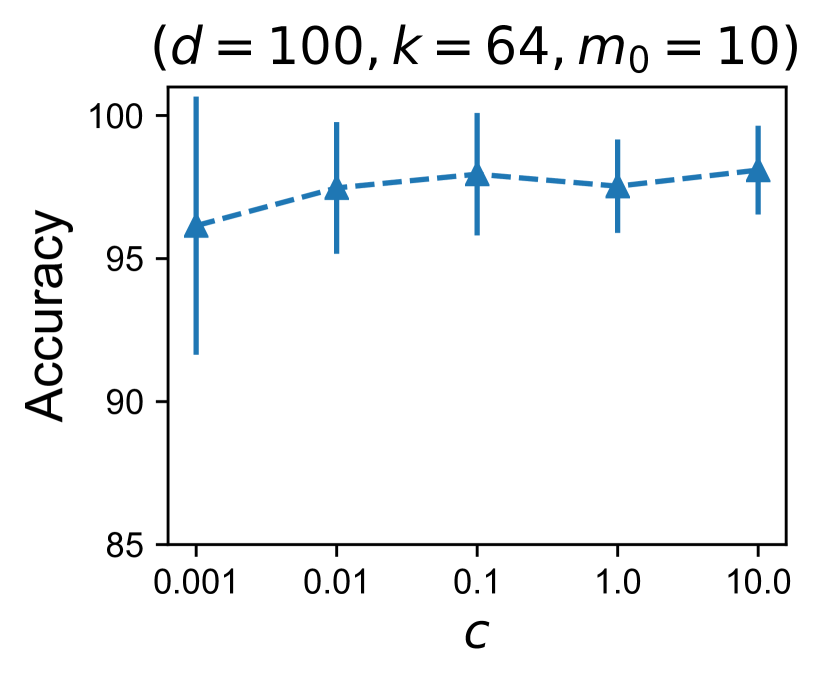
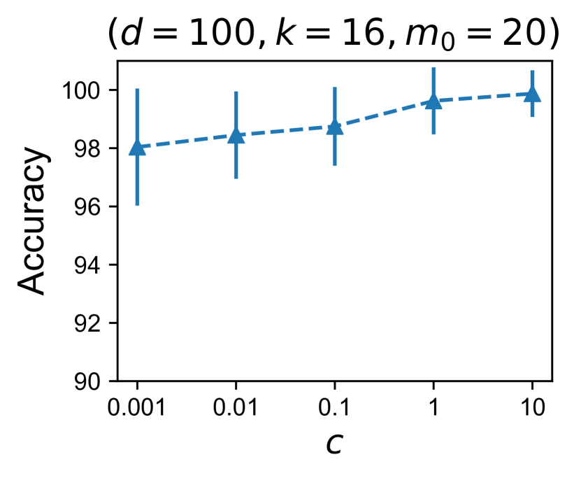
Concretely, in this setup k-FED recovers the target clustering exactly with high probability. To empirically evaluate our theory, we instantiate an simplified instance of the above setup as follows:

Table 1: Clustering accuracy for clustering a mixture of Gaussians. Here for all instances we choose $k^{\prime }=\sqrt{k}$. We can see that the one-shot clustering produced by k-FED agrees with the target clustering with high accuracy, particularly when $k$ is relatively small compared to $d$.

Parameters	Accuracy
$(d=100,k=16,m_0=5,c=100)$	$100.00\pm 0.00$
$(d=100,k=64,m_0=5,c=100)$	$98.82\pm 0.70$
$(d=300,k=64,m_0=5,c=100)$	$99.27\pm 0.73$
$(d=300,k=100,m_0=5,c=100)$	$98.40\pm 0.80$
$(d=300,k=16,m_0=5,c=100)$	$100.00\pm 0.00$

Setup. Again consider the Gaussian components $F_1,\mathrm{\dots },F_k$, and define the set of integers $G_i=\{p\mid (i-1)\times \sqrt{k}\le p\le i\times \sqrt{k}\}$. These sets $G_i$ thus can be used to index the Gaussian components $(F_{(i-1)\sqrt{k}},\mathrm{\dots },F_{i\sqrt{k}})$. For each $G_i$, construct a set of data points $D_i$ by sampling $\text{poly}(dk)$ samples from each component $F_p$ for $p\in G_i$. Thus the set $D_i$ contains $\sqrt{k}\cdot \text{poly}(dk)$ samples $(w_r=\frac{1}{k},\forall r)$. Pick $m_0$ and for each set of data points $D_i$, distribute the data among $m_0$ devices such that each device receives exactly $\frac{1}{m_0}\cdot \text{poly}(dk)$ samples. We now run k-FED on this setup and measure the quality of the clustering averaged over 10 runs, (shown in Table 1). As one would expect, the clustering produced by k-FED agrees strongly with the target clustering. Note that by construction all devices with data from the same set $G_i$ contain data from the same set of Gaussian components. Further, devices with data from different sets $G_i$ have no common Gaussian component. Thus all cluster pairs within the same set $G_i$ are active cluster pairs and there are $\sqrt{k}\left(\genfrac{}{}{0pt}{}{\sqrt{k}}{2}\right)$ such pairs. Moreover, any pair $(r,s)$ such that $r\in G_i$, $s\in G_j$ $i\ne j$ form an inactive cluster pair and there are $\left(\genfrac{}{}{0pt}{}{k}{2}\right)-\sqrt{k}\left(\genfrac{}{}{0pt}{}{\sqrt{k}}{2}\right)=O(k^2)$ such pairs. These need only satisfy the weaker inactive separation requirement.

Figure 1: Impact of the separation constant $c$ on the clustering accuracy when clustering a mixture of Gaussians. Even for relatively small values of $c$, for the case of data generated from a mixture of Gaussians, k-FED can recover highly accurate clustering with decreasing variance across runs.

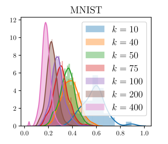
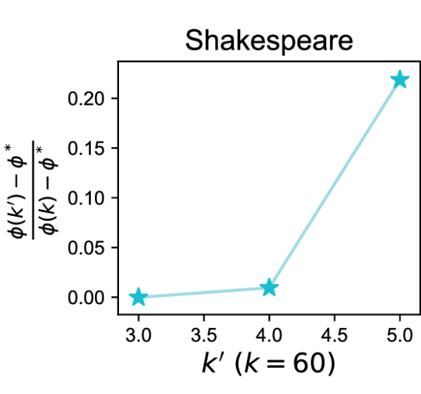
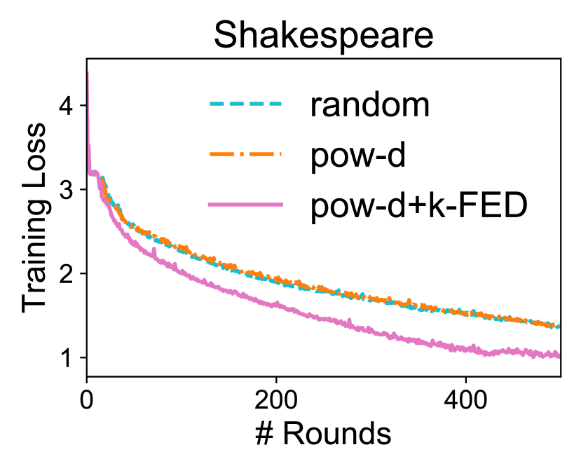
Note that while we prescribe $c\ge 100$ for our arguments to hold, Figure 1 demonstrates that clustering can be recovered even in settings where $c$ is much smaller.

4.2 Empirical Evaluation on Real Data

In this section, we empirically explore k-FED and the related analyses from Section 3. First, we validate our theoretical results, showing that clustering over structured (heterogeneous) partitions can improve clustering performance relative to clustering over random, IID partitioned data. Second, we explore the effect of one-shot clustering relative to more communication-intensive baselines. Finally, we investigate practical applications of one-shot clustering in terms of client sampling and personalized federated learning.

4.2.1 Properties of k-FED

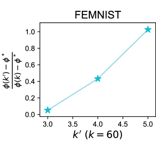
Benefits of Heterogeneity (Def. 3.2). We compare the performance of k-FED on two different partitions of data among devices: (i) one with IID random partitions, and (ii) another with structured partitions. To generate the underlying structured partition for this experiment we use the following heuristic. First, we cluster all the data into $k$ clusters for a range of values of $k$. For each $k$, we take the clustering we have as the target clustering $𝒯$, and construct the data matrix $A$ and the matrix of centers $C$. Finally, for each pair of cluster means ${\mu }_r,{\mu }_s$, we compute the quantity $\frac{\parallel {\mu }_r-{\mu }_s\parallel }{2\sqrt{m_0}({\mathrm{\Delta }}_r+{\mathrm{\Delta }}_s)}$, the ratio of the actual separation of the cluster mean to the required active separation. We pick a value of $k$ at which a large number of clusters are reasonably well separated (see Appendix B, Figure 5). We call this our oracle clustering. Now to generate the IID partition for (i), we randomly distribute this data among $Z$ devices. To generate the structured partition for (ii), we divide the data among $Z$ devices such that each device receives only data from a random subset of no more than $k^{\prime }$ clusters. For each value of $k^{\prime }$, we cluster the data for both cases over the devices using k-FED and compute the $k$-means cost. Let ${\varphi }^{\ast }$ denotes the $k$-means cost of the original oracle clustering. Let $\varphi (k^{\prime })$ denote the $k$-means cost when $k^{\prime }$ clusters are assigned to each device. Figure 2 presents the relative cost ratio between the cost change in structured partitions ($\varphi (k^{\prime })-{\varphi }^{\ast }$) and random partitions ($\varphi (k)-{\varphi }^{\ast }$).

We perform this experiment on the FEMNIST and Shakespeare datasets (Caldas et al., 2018) (see Appendix B for details). It can be seen from the results plotted in Figure 2 that clustering on structured splits achieves a cost closer to that of the oracle partition compared to the cost achieved on the IID random partition. We note that the separation achieved in real datasets is much smaller than required even with this careful construction (Appendix B). Even still, our experiments demonstrate that heterogeneity can benefit federated clustering on common benchmarks.

Figure 2: The $k$-means cost under structured partitions ($\varphi (k^{\prime })$) is closer to the cost of oracle clustering (${\varphi }^{\ast }$) than that under random partitions ($\varphi (k)$). As heterogeneity increases ($k^{\prime }$ decreases), the benefits of structured partitions are becoming more significant, with $\varphi (k^{\prime })-{\varphi }^{\ast }\ll \varphi (k)-{\varphi }^{\ast }$.

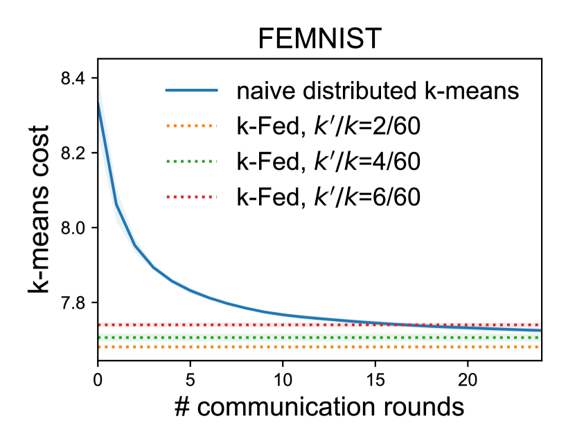
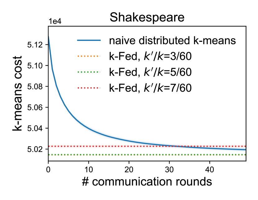
Communication-Efficiency. One advantage of the proposed method is that it requires only a single round of communication. Given this, it is natural to wonder how the performance of k-FED would compare with other, more communication-intensive clustering baselines. In particular, a common way to solve $k$-means in distributed settings is to simply parallelize the cluster assignment and cluster mean calculations at each step. Here, we show that for different partitions of the dataset with multiple values of $k^{\prime }$, our one-shot method $k$-FED is able to produce similar clustering outputs (in terms of the $k$-means cost; lower is better) as naive distributed $k$-means, which requires multiple communication rounds. Here we use the same oracle clustering as the previous experiment to construct our device data.

Figure 3: $k$-FED (using just one communication round) is able can provide similar clustering quality as naive distributed $k$-means.

4.2.2 Applications of $k$-Fed

Personalized FL. Compared with fitting a single global model to data across all device, jointly learning personalized (separate but related) models can boost the effective sample size while adapting to the heterogeneity in federated networks (e.g., Smith et al., 2017; Mansour et al., 2020).

Ghosh et al. (2020) recently proposed an algorithm to learn models over federated networks where devices are partitioned into clusters when the clustering information is unavailable. Consider a supervised learning problem that each cluster of devices want to solve and assume the number of clusters $k$ is known. Their method, the Iterative Federated Clustering Algorithm (IFCA), in its first step initializes $k$ models $(m_1,\mathrm{\dots },m_k)$, one for each cluster. At the start of each round, all $k$ models are sent to the devices. Each device picks the model that minimizes a loss function on its locally available data. The device can be configured to now either compute and transmit the gradient of the loss function of this model or it can perform a few model updates locally and send the updated model to the central server. As the last step of the round, for each model $m_i$ $i\in [k]$, all the devices that picked this model are identified. All these devices are assigned cluster id $i$. Model $m_i$ then is updated by either model averaging or gradient averaging using the information sent by devices in cluster $i$.

Table 2: Test accuracy of rotated MNIST on three methods. Training personalized models based on the clustering information output by k-FED achieves the same performance of IFCA, without the high computation and communication overhead of IFCA when $k^{\prime }=1$. For $k^{\prime }=2$, the performance of k-FED degrades much less when compared to that of IFCA.

	Global	IFCA	$k$-FED
100 devices ($k^{\prime }=1$)	95.0	98.0	98.0
200 devices ($k^{\prime }=1$)	94.5	97.2	97.8
100 devices ($k^{\prime }=2$)	95.3	95.6	97.1
200 devices ($k^{\prime }=2$)	94.5	95.1	96.4

We instantiate IFCA on the problem of learning personalized models for clusters. As in (Ghosh et al., 2020), we use the MNIST dataset for this experiment. We construct $k=4$ clusters by $0,90,180$ and $270$ degree rotations and distribute them among devices. Note that in the setup for IFCA, each device only contains data from a single cluster (since we are clustering devices and not individual data points). Thus we set $k^{\prime }=1$ and compare IFCA with a simple k-FED based method: We first perform one-shot clustering to obtain an initial clustering and then we use FedAvg (McMahan et al., 2017) to learn one model per cluster. As a baseline, we also learn a single global model and include it for comparison. As can be seen from the test accuracies in Table 2 ($k^{\prime }=1$), k-FED is competitive with IFCA. Moreover, k-FED has the additional advantage that once the cluster identities have been assigned, we only need to transmit one model instead of the $k$ models that are transmitted with IFCA.

Since k-FED clusters data, the k-FED + FedAvg approach can also handle cases where there are data from multiple clusters on the same device. Table 2 ($k^{\prime }=\sqrt{k}=2$) shows the test accuracy on such a partition. Here we observe the performance of IFCA degrade when compared to k-FED.

Client Selection. Finally, we demonstrate that the clustering information produced by $k$-FED is a useful prior for client selection applications (Cho et al., 2020). In practice, cross-device federated optimization algorithms need to tolerate partial device participation (Kairouz et al., 2019). Intuitively, incorporating information from ‘representative’ devices at each communication round may speed up the convergence of learning tasks over federated networks as opposed to randomly sampling devices. When randomly sampling, similar and potentially redundant clients can be selected. A recent device selection method proposes to additionally select the devices with large training losses among those randomly-selected subset of devices (Cho et al., 2020) to help with convergence speed. We combine $k$-FED with this approach by further filtering out the devices coming from the same clusters. Note that $k$-FED does not add significant additional overhead to the baseline algorithm as it only requires running one-shot clustering before training. The results are shown in Figure 4. We see that leveraging the underlying structure learnt by $k$-FED can boost convergence on these realistic federated benchmarks.

Figure 4: Additional clustering information provided by $k$-FED can help achieve faster convergence than recent client selection techniques pow-d (Cho et al., 2020).

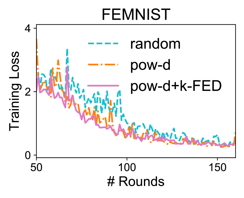
Similar to Cho et al. (2020), we also observe that for the experiments in Figure 4, the variance of test performance across all devices has been reduced using client selection strategies favoring more informative (potentially more underrepresented) clients compared with that of random selection. For instance, on FEMNIST, the variance of final test accuracies is reduced by 35% when using k-fed combined with pow-d instead of random selection. This may be useful in scenarios where we wish to impose notions fairness for federated learning (Mohri et al., 2019; Li et al., 2020c).

5 Conclusion

In this work, we provide an example of how heterogeneity in federated networks can be beneficial, by rigorously analyzing the effects of heterogeneity on a simple, one-shot variant of Lloyd’s algorithm for distributed clustering. Our proposed method, k-FED, addresses common practical concerns in federated settings, such as high communication costs, stragglers, and device failures. We believe that other, specific notions of heterogeneity—together with careful analyses—may provide benefits for a plethora of other problems in federated learning, which is an interesting direction of future work.

6 Acknowledgements

This work was supported in part by the National Science Foundation Grant IIS1838017, a Google Faculty Award, a Facebook Faculty Award, and the CONIX Research Center. Any opinions, findings, and conclusions or recommendations expressed in this material are those of the author(s) and do not necessarily reflect the National Science Foundation or any other funding agency.

Appendix A Proofs

A.1 Proving Theorem 3.1 (Main Theorem)

Before we proceed to proving Theorem 3.1, we first establish a few preliminary results. Let $𝒯=(T_1,\mathrm{\dots },T_k)$ be our target clustering and let $T_r^{(z)}$ be the subset of points of a cluster $T_r$ on device $z$. For any point, $A_i^{(z)}$ on device $z$, let $c(A_i^{(z)})$ denote the index of the cluster it belongs to. That is,

$$A_i^{(z)}\in T_{c(A_i^{(z)})}^{(z)}\subseteq T_{c(A_i^{(z)})}.$$

Also recall the definition of matrix $C$, the matrix of means. Here the $i$-th row of $C$ contains the mean of the cluster which contains data points $A_i$, i.e. $C_i=\mu (T_{c(A_i)})$. Our first lemma bounds how far the ‘local’ cluster mean $\mu (T_r^{(z)})$ can deviate from $\mu (T_r)$.

Lemma 2 (Lemma 5.2 in Kumar & Kannan (2010)).

Let $T_r^{(z)}$ be a subset of $T_r$ on device $z$. Let $\mu (T_r^{(z)})$ denote the mean of the points indexed by $T_r^{(z)}$. Then,

${\parallel \mu (T_r^{(z)})-\mu (T_r)\parallel }_2\le {\displaystyle \frac{\parallel A-C\parallel }{\sqrt{|T_r^{(z)}|}}}.$

Proof.

Let $A^{(z)}$ be the sub-matrix of $A$ on device $z$ and let ${\tilde{C}}^{(z)}$ be the corresponding sub-matrix of our matrix of means $C$. Let $u$ be an indicator vector for points in $T_r^{(z)}$. Observe that,

${\parallel |T_r^{(z)}|(\mu (T_r^{(z)})-{\mu }_r)\parallel }_2$ $={\parallel (A^{(z)}-{\tilde{C}}^{(z)})\cdot u\parallel }_2$

$\le \parallel A^{(z)}-{\tilde{C}}^{(z)}\parallel {\parallel u\parallel }_2$

$\le \parallel A-C\parallel \sqrt{\left|T_r^{(z)}\right|}.$

Here, for the last inequality, we note that $(A^{(z)}-{\tilde{C}}^{(z)})$ contains a subset of rows of $(A-C)$, and therefore $\parallel A^{(z)}-{\tilde{C}}^{(z)}\parallel \le \parallel A-C\parallel$. ∎

Now consider the local clustering problem on each device $z$. The device has a data matrix $A^{(z)}$, whose rows are a subset of $A$. Let $T_1^{(z)},T_2^{(z)},\mathrm{\dots },T_k^{(z)}$ be subsets of $T_1,T_2,\mathrm{\dots },T_k$ on this device, such that no more than $k^{\prime }$ of them are non-empty. Construct a matrix $C^{(z)}$, of the same dimensions as $A^{(z)}$ where for each row of $A^{(z)}$, the corresponding row of $C^{(z)}$ contains the mean of the local cluster the point belongs to. That is, the $i$-th row of $C^{(z)}$ contains $\mu (T_{c(A_i^{(z)})}^{(z)})$. Using this next lemma, we bound the operator norm of the matrix $(A^{(z)}-C^{(z)})$, in terms of $(A-C)$.

Lemma 3.

Let $T_1^{(z)},T_2^{(z)},\mathrm{\dots }{T}_k^{(z)}$ be subsets of target cluster that reside on a device such that $k^{\prime }$ of them are non-empty. Let $A^{(z)}$ be the corresponding $n^{(z)}\times d$ data matrix. Let $C^{(z)}$ be the corresponding matrix of means; that is each row $C_i^{(z)}=\mu (T_{c(A_i^z)}^z)$. Then,

$$\parallel A^{(z)}-C^{(z)}\parallel \le 2\sqrt{k^{\prime }}\parallel A-C\parallel .$$

Proof.

Let ${\tilde{C}}^{(z)}$ be an $n^{(z)}\times d$ matrix where ${\tilde{C}}_i^{(z)}=\mu (T_{c(A_i^{(z)})})$. First, consider a unit vector $u$ along the top singular direction and observe that:

${\parallel {\tilde{C}}^{(z)}-C^{(z)}\parallel }^2$ $={\displaystyle \sum _{r=1}^k}|T_r^{(z)}|{\left(\left(\mu (T_r^{(z)})-\mu (T_r)\right)\cdot u\right)}^2$

$\le {\displaystyle \sum _{r=1}^k}|T_r^{(z)}|{\parallel \mu (T_r^{(z)})-\mu (T_r)\parallel }_2^2$

${\le }_{(a)}{k}^{\prime }{\parallel A-C\parallel }^2.$

Here for inequality $(a)$ we invoke Lemma 2. Also, noting that $\parallel A^{(z)}-{\tilde{C}}^{(z)}\parallel \le \parallel A-C\parallel$, we get,

$\parallel A^{(z)}-C^{(z)}\parallel$ $\le \parallel A^{(z)}-{\tilde{C}}^{(z)}\parallel +\parallel {\tilde{C}}^{(z)}-C^{(z)}\parallel$

$\le (1+\sqrt{k^{\prime }})\parallel A-C\parallel \le 2\sqrt{k^{\prime }}\parallel A-C\parallel .$

∎

We prove Theorem 3.1 in four parts:

1. In the first step we show that satisfying the active separation condition is sufficient to satisfy the Awasthi-Sheffet separation condition required for Lemma 1 (Lemma 4).

2. Next we use Lemma 4 to show that the first step of k-FED (Algorithm-1) will find local centers ${\theta }_r^{(z)}$ that are close to true centers $\mu (T_r^{(z)})$ on device $z$. We state and prove this in Lemma 5.

3. In next step, we show that the process of picking $k$ initial centers in steps 2-6 of k-FED picks exactly one local cluster center ${\theta }_r^{(z)}$ for each cluster $r$. That is, we pick $k$ local centers one corresponding to each target cluster. (Lemma 6)

4. Finally, we argue that with this initialization, the clustering of local cluster centers produced $({\tau }_1,\mathrm{\dots },{\tau }_k)$ has the property that, all local cluster centers corresponding the to the same cluster (say $T_r$) will be in the same set (say ${\tau }_r$). Moreover, no local cluster center corresponding to any $T_s$, $s\ne r$ will be in ${\tau }_r$. As we argue later, this is sufficient for the induced clustering produced by $({\tau }_1,\mathrm{\dots },{\tau }_k)$ to agree with our target clustering $𝒯=(T_1,T_2,\mathrm{\dots })$ up to permutation of labels and missclassifications incurred at the local clustering stage.

Lemma 4.

Let $(T_r,T_s)$ be cluster pairs such that, ${\parallel {\mu }_r-{\mu }_s\parallel }_2\ge 2c\sqrt{m_0}({\mathrm{\Delta }}_r+{\mathrm{\Delta }}_s).$ Let $T_r^z\subseteq T_r$ and $T_s^z\subseteq T_s$ be large subsets on device $z$. Then,

${\parallel {\mu }_r^{(z)}-{\mu }_s^{(z)}\parallel }_2\ge c\sqrt{k^{\prime }}\left({\displaystyle \frac{\parallel A^{(z)}-C^{(z)}\parallel }{\sqrt{n_r^{(z)}}}}+{\displaystyle \frac{\parallel A^{(z)}-C^{(z)}\parallel }{\sqrt{n_s^{(z)}}}}\right).$

Proof.

(Lemma 4) Using the triangle inequality, we have

${\parallel {\mu }_r^{(z)}-{\mu }_s^{(z)}\parallel }_2$ $\ge {\parallel {\mu }_r-{\mu }_s\parallel }_2-{\parallel {\mu }_r^{(z)}-{\mu }_r\parallel }_2-{\parallel {\mu }_s-{\mu }_s^{(z)}\parallel }_2$

$\ge 2c\sqrt{m_0}({\mathrm{\Delta }}_r+{\mathrm{\Delta }}_s)-{\displaystyle \frac{\parallel A-C\parallel }{\sqrt{n_r^{(z)}}}}-{\displaystyle \frac{\parallel A-C\parallel }{\sqrt{n_s^{(z)}}}}$ (5)

using the active separation assumption. Now, expanding the terms can write the left hand side as

${\parallel {\mu }_r^{(z)}-{\mu }_s^{(z)}\parallel }_2$ $\ge 2c\sqrt{m_0}\left(k^{\prime }{\displaystyle \frac{\parallel A-C\parallel }{\sqrt{n_r}}}+k^{\prime }{\displaystyle \frac{\parallel A-C\parallel }{\sqrt{n_s}}}\right)-{\displaystyle \frac{\parallel A-C\parallel }{\sqrt{n_r^{(z)}}}}-{\displaystyle \frac{\parallel A-C\parallel }{\sqrt{n_s^{(z)}}}}$

$\ge \underset{(i)}{\underbrace{\left(2\sqrt{{\displaystyle \frac{m_0{n}_r^{(z)}}{n_r}}}-{\displaystyle \frac{1}{c{k}^{\prime }}}\right)c{k}^{\prime }{\displaystyle \frac{\parallel A-C\parallel }{\sqrt{n_r^{(z)}}}}}}+\underset{(ii)}{\underbrace{\left(2\sqrt{{\displaystyle \frac{m_0{n}_s^{(z)}}{n_s}}}-{\displaystyle \frac{1}{c{k}^{\prime }}}\right)c{k}^{\prime }{\displaystyle \frac{\parallel A-C\parallel }{\sqrt{n_s^{(z)}}}}}}.$

We first only consider the term $(i)$. According to Lemma 3, $\parallel A-C\parallel \ge \frac{1}{2\sqrt{k^{\prime }}}\parallel A^{(z)}-C^{(z)}\parallel$. Using this we can bound $(i)$ as

$$\left(2\sqrt{\frac{m_0{n}_r^{(z)}}{n_r}}-\frac{1}{c{k}^{\prime }}\right)c{k}^{\prime }\frac{\parallel A-C\parallel }{\sqrt{n_r^{(z)}}}\ge \left(2\sqrt{\frac{m_0{n}_r^{(z)}}{n_r}}-\frac{1}{c{k}^{\prime }}\right)c\sqrt{k^{\prime }}\frac{\parallel A^{(z)}-C^{(z)}\parallel }{\sqrt{n_r^{(z)}}}.$$

Now recall that for large cluster subsets $n_r^{(z)}\ge \frac{1}{m_0}{n}_r$ and thus $2\sqrt{\frac{m_0{n}_r^{(z)}}{n_r}}-\frac{1}{c{k}^{\prime }}\ge 2-\frac{1}{c{k}^{\prime }}\ge 1$. This means that we can bound term $(i)$ as,

$$\left(2\sqrt{\frac{m_0{n}_r^{(z)}}{n_r}}-\frac{1}{c{k}^{\prime }}\right)c{k}^{\prime }\frac{\parallel A-C\parallel }{\sqrt{n_r^{(z)}}}\ge c\sqrt{k^{\prime }}\frac{\parallel A^{(z)}-C^{(z)}\parallel }{\sqrt{n_r^{(z)}}}.$$

We get a symmetric expression for term $(ii)$ as well. Using this in equation 5, we get the desired result:

${\parallel {\mu }_r^{(z)}-{\mu }_s^{(z)}\parallel }_2\ge c\sqrt{k^{\prime }}\left({\displaystyle \frac{\parallel A^{(z)}-C^{(z)}\parallel }{\sqrt{n_r^{(z)}}}}+{\displaystyle \frac{\parallel A^{(z)}-C^{(z)}\parallel }{\sqrt{n_s^{(z)}}}}\right).$

∎

Since Algorithm-1 is run locally on each device, it is unaffected by the inactive separation condition, as by definition, subsets of only active cluster pairs exist on each device. This implies that Algorithm-1 solves the local clustering problem successfully. Specifically on device $z$ containing data from some cluster $T_r$, ${\theta }_r^z$ is not too far from $\mu (T_r^{(z)})$. Showing this result is our second step and we state this formally in Lemma 5 below.

Lemma 5.

Let $(T_1^{(z)},\mathrm{\dots },T_k^{(z)})$ be the subsets of $(T_1,\mathrm{\dots },T_k)$ on some device $z$ such that no more than $k^{\prime }$ of them are non-empty. Moreover, assume all non-empty subsets are large, i.e. $|T_r^{(z)}|\ge \frac{1}{m_0}\left|T_r\right|$. Finally, assume that the active separation requirement is satisfied for all active cluster pairs on $z$. Then, on termination of Algorithm-1, for each non-empty $T_r^{(z)}$, we have

$${\parallel {\theta }_r^{(z)}-\mu (T_r^{(z)})\parallel }_2\le \frac{25}{c}\frac{\parallel A^{(z)}-C^{(z)}\parallel }{\sqrt{n_r^z}}\le \frac{50\sqrt{k^{\prime }}}{c}\frac{\parallel A-C\parallel }{\sqrt{n_r^z}},$$

and,

$${\parallel {\theta }_r^{(z)}-\mu (T_r)\parallel }_2\le 2\sqrt{m_0{k}^{\prime }}\frac{\parallel A-C\parallel }{\sqrt{n_r}}\le 2\sqrt{m_0}\lambda .$$

Proof.

First note that the local clustering problem with data matrix $A^{(z)}$ and matrix of centers $C^{(z)}$ satisfies the requirements of Lemma 1. Thus it follows that,

$${\parallel {\theta }_r^{(z)}-\mu (T_r^{(z)})\parallel }_2\le \frac{25}{c}\frac{\parallel A^{(z)}-C^{(z)}\parallel }{\sqrt{n_r^z}}.$$

Now applying Lemma 3 gives us the first statement.

To prove the second statement, we start off with the triangle inequality:

${\parallel {\theta }_r^{(z)}-\mu (T_r)\parallel }_2$ $\le {\parallel {\theta }_r^{(z)}-\mu (T_r^{(z)})\parallel }_2+{\parallel \mu (T_r^{(z)})-\mu (T_r)\parallel }_2$

$\le {\displaystyle \frac{25}{c}}{\displaystyle \frac{\parallel A^{(z)}-C^{(z)}\parallel }{\sqrt{n_r^z}}}+{\displaystyle \frac{\parallel A-C\parallel }{\sqrt{n_r^z}}}.$

Here for the last inequality we used Lemma 2. Now applying Lemma 3 and taking take $c\ge 100$, we get

${\parallel {\theta }_r^{(z)}-\mu (T_r)\parallel }_2$ $\le {\displaystyle \frac{50\sqrt{k^{\prime }}}{c}}{\displaystyle \frac{\parallel A-C\parallel }{\sqrt{n_r^z}}}+{\displaystyle \frac{\parallel A-C\parallel }{\sqrt{n_r^z}}}$

$\le \left({\displaystyle \frac{50}{c}}+{\displaystyle \frac{1}{\sqrt{k^{\prime }}}}\right)\sqrt{k^{\prime }}{\displaystyle \frac{\parallel A-C\parallel }{\sqrt{n_r^z}}}$

$\le 2\sqrt{k^{\prime }}{\displaystyle \frac{\parallel A-C\parallel }{\sqrt{n_r^z}}}\le 2\sqrt{m_0{k}^{\prime }}{\displaystyle \frac{\parallel A-C\parallel }{\sqrt{n_r}}}$

$\le 2\sqrt{m_0}\lambda .$

∎

This means that for a fixed $r$, all the ${\theta }_r^{(z)}$ received at the central server from devices $z\in [Z]$ are ‘close’ to $\mu (T_r)$.

The next step is to show that in the $k$ initial centers k-FED picks in steps 2-6, there is exactly one corresponding to each target cluster $T_i$. We will show later that this is sufficient for the final step of the algorithm to correctly assign local cluster centers to the correct partition.

Lemma 6.

Let $𝒯=(T_1,\mathrm{\dots },T_k)$ be our target clustering. Assume all active cluster pairs and inactive cluster pairs satisfy their separation requirements. Further let $n_{\min }\ge \frac{4}{c^2{k}^{\prime }}{n}_{\max }$. Then at the end of step 6 of k-FED, for every target cluster $T_r$, there exists an ${\theta }_s^{(z)}\in M$ such that ${\theta }_s^{(z)}=\mu (T_s^{(z)})$ for some $z\in [Z]$.

Before we proceed to proving this lemma, we state and prove a lower bound on how close a local cluster center ${\theta }_r^{(z)}$ can be to some cluster mean $\mu (T_s)$ for $s\ne r$:

Lemma 7.

Let ${\theta }_r^{(z)}:=\mu (T_r^{(z)})$. The for any $s\ne r$, $z^{\prime }\in [Z]$,

$${\parallel {\theta }_r^{(z)}-{\theta }_s^{(z^{\prime })}\parallel }_2\ge 6\sqrt{m_0}\lambda .$$

Proof.

First, from the triangle inequality note that,

$${\parallel {\theta }_r^{(z)}-{\theta }_s^{(z^{\prime })}\parallel }_2\ge {\parallel {\mu }_r-{\mu }_s\parallel }_2-{\parallel {\mu }_r-{\theta }_r^{(z)}\parallel }_2-{\parallel {\mu }_s-{\theta }_s^{(z^{\prime })}\parallel }_2.$$

Using Lemma 5 and our inactive separation assumption we bound the right hand side further as,

${\parallel {\mu }_r-{\mu }_s\parallel }_2-{\parallel {\mu }_r-{\theta }_r^{(z)}\parallel }_2-{\parallel {\mu }_s-{\theta }_s^{(z^{\prime })}\parallel }_2$ $\ge 10\sqrt{m_0{k}^{\prime }}{\displaystyle \frac{\parallel A-C\parallel }{\sqrt{n_{\min }}}}-4\sqrt{m_0{k}^{\prime }}{\displaystyle \frac{\parallel A-C\parallel }{\sqrt{n_r}}}$

$\ge 6\sqrt{m_0{k}^{\prime }}{\displaystyle \frac{\parallel A-C\parallel }{\sqrt{n_{\min }}}}\ge 6\sqrt{m_0}\lambda ,$

as desired. ∎

Proof.

(Lemma 6) Let $M_t$ denote the set $M$ in step 2-6 of k-FED, after picking the first $t$ points $(1\le t\le k)$. Let us denote the point k-FED selects in iteration $t$ as ${\theta }_t$. That is,

$${\theta }_t\leftarrow \underset{z\in [Z],i\in [k]}{\arg \max }{d}_{M_{t-1}}({\theta }_i^{(z)}).$$

We will show that the set $M_t$ contains $t$ points corresponding to $t$ different target clusters at every iteration $t$. This invariant holds trivially at $t=1$. Assume the statement first became false at some . Let the point ${\theta }_{t^{\prime }}$ correspond to a local cluster mean from cluster $T_r$. Then there must exist some such that ${\theta }_{t^{\prime \prime }}$ also correspond to a local cluster mean from $T_r$. Further, there must exist some cluster $s\ne r$ such that ${\theta }_s^{(z)}\notin M_{t^{\prime }}$ for any $z\in [Z]$.

Now by definition of $d_{M_{t-1}}({\theta }_{t^{\prime }})$, we have

$d_{M_{t-1}}({\theta }_{t^{\prime }})$ $=\underset{\theta \in M_{t-1}}{\min }{\parallel {\theta }_{t^{\prime }}-\theta \parallel }_2$

$\le {\parallel {\theta }_{t^{\prime }}-{\theta }_{t^{\prime \prime }}\parallel }_2$

${\le }_{(a)}{\parallel {\theta }_{t^{\prime }}-\mu (T_r)\parallel }_2+{\parallel \mu (T_r)-{\theta }_{t^{\prime \prime }}\parallel }_2$

${\le }_{(b)}4\sqrt{m_0{k}^{\prime }}{\displaystyle \frac{\parallel A-C\parallel }{\sqrt{n_r}}}\le 4\sqrt{m_0}\lambda .$ (6)

Here inequality (a) follows from the triangle inequality and (b) follows from Lemma 5.

Now consider ${\theta }_s^{(z)}$ for any $z$. Since no other local cluster center from $T_s$ is contained in $M_t$, from Lemma 7 we conclude that for every $\theta \in M_{t-1}$,

${\parallel {\theta }_s^{(z)}-\theta \parallel }_2\ge 6\sqrt{m_0}\lambda .$

But this means that $d_{M_{t-1}}({\theta }_{t^{\prime }})\le 4\sqrt{m_0}\lambda \le 6\sqrt{m_0}\lambda \le d_{M_{t-1}}({\theta }_s^{(z)})$ leading to a contradiction based on the definition of ${\theta }_{t^{\prime }}$. This completes our argument. ∎

Now we are ready to prove our main Theorem 3.1.

Proof.

From Lemma 6, we know that the set $M$ at the end of step 6 of k-FED contains exactly one center corresponding to each target clustering. Let the local cluster center ${\tilde{\theta }}_r\in M$ correspond to the cluster $T_r$. Observe that for any $z\in [Z]$,

${\parallel {\theta }_r^z-{\tilde{\theta }}_r\parallel }_2$ $\le {\parallel {\theta }_r^z-{\mu }_r\parallel }_2+{\parallel {\mu }_r-{\tilde{\theta }}_r\parallel }_2$

$\le 4\sqrt{m_0}\lambda ,$

using Lemma 7. Further, for any $s\ne r$,

${\parallel {\theta }_s^z-{\tilde{\theta }}_r\parallel }_2$ $\ge 6\sqrt{m_0}\lambda .$

This means that for every $r$ and $z\in [Z]$, ${\theta }_r^z$ is closer to the corresponding initial center ${\tilde{\theta }}_r$ than to any other initial center ${\tilde{\theta }}_s$, $s\ne r$. Let ${\tau }_r$ be the set of local cluster centers assigned to $\widetilde{{\theta }_r}$. Then it can be seen that ${\tau }_r$ only contains local cluster centers ${\theta }_r^{(z)}$ for all devices $z$, i.e. ${\tau }_r$ contains all the device cluster centers corresponding to target cluster $T_r$.

Now consider the definition of k-FED induced clustering (Definition 3.3), where we define

$$T_r^{\prime }=\{i:A_i^{(z)}\in U_s^{(z)}\text{and}{\theta }_s^{(z)}\in {\tau }_r\}.$$

In this case, we know that only local cluster centers corresponding to cluster $T_r$ is contained in ${\tau }_r$. Thus our induced cluster $T_r^{\prime }$ becomes,

$$T_r^{\prime }=\{i:A_i^{(z)}\in U_r^{(z)}\}.$$

Now from Lemma 1 we know that on each device the sets $(U_1^{(z)},\mathrm{\dots },U_{k^{\prime }}^{(z)})$ and $(T_1^{(z)},\mathrm{\dots },T_{k^{\prime }}^{(z)})$ only differ on at most $O(\frac{1}{c^2})n^{(z)}$. Summing this error over all devices $z$, we see that our induced clustering $(T_1^{\prime },\mathrm{\dots },T_k^{\prime })$ and the target clustering $(T_1,\mathrm{\dots },T_k)$ differ only on $O(\frac{1}{c^2})n$ points. Finally, if all the local points satisfy their respective proximity condition (Definition 3.1), then no points are missclassified. This concludes our proof. ∎

A.2 Running Time of k-FED and Handling New Devices

We now analyze the running time of k-FED steps 2-8. Since step 1 is running Algorithm-1 on individual devices, we do not include the running time of this step as part of our analysis. Note that with the separation assumptions in place, Algorithm-1 will converge in polynomial time. However, as observed in practise, Lloyd like methods typically only take a few iterations to terminate.

Theorem A.1.

Steps 2-8 of k-FED takes $O(Z{k}^{\prime }\cdot k^2)$ pairwise distance computations to terminate. Further, after the set $M$ in step 6 has been computed, new local cluster centers ${\mathrm{\Theta }}^{(z)}$ from a yet unseen device $z$ can be correctly assigned in $O(k^{\prime }\cdot k)$ distance computations.

Proof.

(Theorem 3.2) The proof of the first part follows from a simple step by step analysis. Step 1 can be performed in $O(1)$. Step 2-6 executes exactly $k$ times. At each iteration $t$, $(1\le t\le k)$, we compute the distance of all device cluster centers, of which there are most $Z{k}^{\prime }$, to the points in $M_{t-1}$. Thus at iteration $t$, this can be implemented with $Z{k}^{\prime }\cdot t$ distance computations. Summing over all $t$, we see that steps 2-6 can run in $O(Z{k}^{\prime }\cdot k^2)$ distance computations. Finally, step 7 requires us to assign all the $Z{k}^{\prime }$ device cluster centers to one of the $k$ initial points in $M$. This can be implemented in $O(Z{k}^{\prime }\cdot k)$ distance computations. Thus the overall complexity in terms of pairwise distance computations is $O(Z{k}^{\prime }\cdot k^2)$.

The second part of the statement follows from noting that for each ${\theta }_r^{(z)}\in {\mathrm{\Theta }}^{(z)}$, the nearest point in set $M$ must be the initial center ${\tilde{\theta }}_r$ we picked as was demonstrated in the proof of Theorem 3.1. Thus every ${\theta }_r^{(z)}\in {\mathrm{\Theta }}^{(z)}$ is assigned to the correct partition ${\tau }_r$ as required. ∎

A.3 Separating Data from Mixture of Gaussian

We now prove Theorem 4.1. Recall that we are working in the setting where $k^{\prime }\le \sqrt{k}$. Our proof builds on results from Lemma 6.3, Kumar & Kannan (2010).

Proof.

First consider an active cluster pair $r,s$. Based on our separation requirement, we have:

${\parallel {\mu }_r-{\mu }_s\parallel }_2$ $\ge {\displaystyle \frac{2c\sqrt{k{m}_0}{\sigma }_{\max }}{\sqrt{w_{\min }}}}\text{polylog}\left({\displaystyle \frac{d}{w_{\min }}}\right)$

$\ge 2c\sqrt{k{m}_0}{\displaystyle \frac{{\sigma }_{\max }\sqrt{n}}{\sqrt{w_{\min }n}}}\text{polylog}\left({\displaystyle \frac{d}{w_{\min }}}\right).$

We further simplify the right hand to get,

$${\parallel {\mu }_r-{\mu }_s\parallel }_2\ge c\sqrt{k{m}_0}{\sigma }_{\max }\sqrt{n}\left(\frac{1}{\sqrt{w_{r}n}}+\frac{1}{\sqrt{w_{s}n}}\right)\text{polylog}\left(\frac{d}{w_{\min }}\right).$$

Now note the number of points from each component $F_r$ is very close to $w_r{n}_r$ with very high probability. Here $w_r$ is the mixing weight of component $r$ and $n_r$ is the number of data points. Using this, with high probability we have

$${\parallel {\mu }_r-{\mu }_s\parallel }_2\ge c\sqrt{k{m}_0}{\sigma }_{\max }\sqrt{n}\left(\frac{1}{\sqrt{n_r}}+\frac{1}{\sqrt{n_s}}\right)\text{polylog}\left(\frac{d}{w_{\min }}\right).$$

Further, it can be shown that $\parallel A-C\parallel$ is $O\left({\sigma }_{\max }\sqrt{n}\cdot \text{polylog}\left(\frac{d}{w_{\min }}\right)\right)$ with high probability (see (Dasgupta et al., 2007)). Thus we conclude that, with high probability

$${\parallel {\mu }_r-{\mu }_s\parallel }_2\ge c\sqrt{k{m}_0}\left(\frac{\parallel A-C\parallel }{\sqrt{n_r}}+\frac{\parallel A-C\parallel }{\sqrt{n_s}}\right).$$

Thus the active separation requirement is satisfied. The proof for the inactive separation condition is similar. Finally, the proximity condition follows from the concentration properties of Gaussians. ∎

Appendix B Experimental Details

B.1 Datasets

For all experiments involving real data, we use the EMNIST, FEMNIST, and Shakespeare datasets. These datasets and their corresponding models are available at the LEAF benchmark: https://leaf.cmu.edu/. For client selection experiments, we manually partition a subset of FEMNIST (first 10 classes) by assigning 2 classes to each device. There are 500 devices in total. Both the number of training samples across all devices and the number of training samples per class within each device follow a power law. We use the natural partition of Shakespeare where each device corresponds to a speaking role in the plays of William Shakespeare. We randomly sample 109 users from the entire dataset. For personalization experiments, following Ghosh et al. (2020), we use a CNN-based model with one hidden layer and 200 hidden units trained with a learning rate of $0.01$ and $10$ local updates on each device.

B.2 Choosing $k$ Based on Separation

As mentioned in Section 4.2, to create our oracle clustering, we compute the quantity $c_{rs}=\frac{\parallel {\mu }_r-{\mu }_s\parallel }{2\sqrt{m_0}({\mathrm{\Delta }}_r+{\mathrm{\Delta }}_s)}$ for each cluster pairs $(r,s)$, for every candidate value of $k$ we are considering. We construct a distribution plot of these $c_{rs}$. An example of such a plot for the MNIST dataset is provided in Figure 5. As can be seen here, for all values of $k$, the relative separation is quite small. Thus even for this oracle clustering, the actual separation between cluster means is small. To pick a $k$ for our oracle clustering, we pick a fixed value $c_0$ (say $0.5$) and then pick the value of $k$ which leads to maximum fraction of cluster pairs $(r,s)$ to have $c_{rs}>c_0$.

Figure 5: Distribution plot of $c_{rs}$, for various values of $k$ on the MNIST dataset. As can be seen, for most cluster pairs, indicating that the separation between them is relatively small.

References

- Arthur & Vassilvitskii (2006) Arthur, D. and Vassilvitskii, S. How slow is the k-means method? In Proceedings of the Twenty-Second Annual Symposium on Computational Geometry, 2006.
- Awasthi & Sheffet (2012) Awasthi, P. and Sheffet, O. Improved spectral-norm bounds for clustering. In Approximation, Randomization, and Combinatorial Optimization. Algorithms and Techniques. 2012.
- Bachem et al. (2018) Bachem, O., Lucic, M., and Krause, A. Scalable k-means clustering via lightweight coresets. In International Conference on Knowledge Discovery & Data Mining, 2018.
- Bahmani et al. (2012) Bahmani, B., Moseley, B., Vattani, A., Kumar, R., and Vassilvitskii, S. Scalable k-means+. Proceedings of the VLDB Endowment, 2012.
- Balcan et al. (2013) Balcan, M.-F., Ehrlich, S., and Liang, Y. Distributed -means and -median clustering on general topologies. In Advances in Neural Information Processing Systems, 2013.
- Bateni et al. (2014) Bateni, M., Bhaskara, A., Lattanzi, S., and Mirrokni, V. Distributed balanced clustering via mapping coresets. In Advances in Neural Information Processing Systems, 2014.
- Caldas et al. (2018) Caldas, S., Duddu, S. M. K., Wu, P., Li, T., Konečnỳ, J., McMahan, H. B., Smith, V., and Talwalkar, A. Leaf: A benchmark for federated settings. arXiv preprint arXiv:1812.01097, 2018.
- Cho et al. (2020) Cho, Y. J., Wang, J., and Joshi, G. Client selection in federated learning: Convergence analysis and power-of-choice selection strategies. arXiv preprint arXiv:2010.01243, 2020.
- Dasgupta et al. (2007) Dasgupta, A., Hopcroft, J., Kannan, R., and Mitra, P. Spectral clustering with limited independence. In Proceedings of the Eighteenth Annual ACM-SIAM Symposium on Discrete Algorithms, 2007.
- Datta et al. (2005) Datta, S., Giannella, C., Kargupta, H., et al. K-means clustering over peer-to-peer networks. In International Workshop on High Performance and Distributed Mining, 2005.
- Dhillon & Modha (2002) Dhillon, I. S. and Modha, D. S. A data-clustering algorithm on distributed memory multiprocessors. In Large-Scale Parallel Data Mining. 2002.
- Ester et al. (1996) Ester, M., Kriegel, H.-P., Sander, J., Xu, X., et al. A density-based algorithm for discovering clusters in large spatial databases with noise. In International Conference on Knowledge Discovery & Data Mining, 1996.
- Feldman et al. (2012) Feldman, D., Sugaya, A., and Rus, D. An effective coreset compression algorithm for large scale sensor networks. In International Conference on Information Processing in Sensor Networks, 2012.
- Ghosh et al. (2019) Ghosh, A., Hong, J., Yin, D., and Ramchandran, K. Robust federated learning in a heterogeneous environment. arXiv preprint arXiv:1906.06629, 2019.
- Ghosh et al. (2020) Ghosh, A., Chung, J., Yin, D., and Ramchandran, K. An efficient framework for clustered federated learning. Advances in Neural Information Processing Systems, 2020.
- Januzaj et al. (2004) Januzaj, E., Kriegel, H.-P., and Pfeifle, M. Dbdc: Density based distributed clustering. In International Conference on Extending Database Technology, 2004.
- Kairouz et al. (2019) Kairouz, P., McMahan, H. B., Avent, B., Bellet, A., Bennis, M., Bhagoji, A. N., Bonawitz, K., Charles, Z., Cormode, G., Cummings, R., et al. Advances and open problems in federated learning. arXiv preprint arXiv:1912.04977, 2019.
- Kargupta et al. (2001) Kargupta, H., Huang, W., Sivakumar, K., and Johnson, E. Distributed clustering using collective principal component analysis. Knowledge and Information Systems, 2001.
- Kumar & Kannan (2010) Kumar, A. and Kannan, R. Clustering with spectral norm and the k-means algorithm. In Annual Symposium on Foundations of Computer Science, 2010.
- Li et al. (2020a) Li, T., Sahu, A. K., Talwalkar, A., and Smith, V. Federated learning: Challenges, methods, and future directions. IEEE Signal Processing Magazine, 2020a.
- Li et al. (2020b) Li, T., Sahu, A. K., Zaheer, M., Sanjabi, M., Talwalkar, A., and Smith, V. Federated optimization in heterogeneous networks. In Proceedings of Machine Learning and Systems, 2020b.
- Li et al. (2020c) Li, T., Sanjabi, M., Beirami, A., and Smith, V. Fair resource allocation in federated learning. In International Conference on Learning Representations, 2020c.
- Lloyd (1982) Lloyd, S. Least squares quantization in pcm. IEEE Transactions on Information Theory, 1982.
- Mansour et al. (2020) Mansour, Y., Mohri, M., Ro, J., and Suresh, A. T. Three approaches for personalization with applications to federated learning. arXiv preprint arXiv:2002.10619, 2020.
- McMahan et al. (2017) McMahan, B., Moore, E., Ramage, D., Hampson, S., and y Arcas, B. A. Communication-efficient learning of deep networks from decentralized data. In Artificial Intelligence and Statistics, 2017.
- McSherry (2001) McSherry, F. Spectral partitioning of random graphs. In Symposium on Foundations of Computer Science, 2001.
- Mohri et al. (2019) Mohri, M., Sivek, G., and Suresh, A. T. Agnostic federated learning. In International Conference on Machine Learning, 2019.
- Ostrovsky et al. (2013) Ostrovsky, R., Rabani, Y., Schulman, L. J., and Swamy, C. The effectiveness of lloyd-type methods for the k-means problem. Journal of the ACM, 2013.
- Sattler et al. (2020) Sattler, F., Müller, K.-R., and Samek, W. Clustered federated learning: Model-agnostic distributed multitask optimization under privacy constraints. IEEE Transactions on Neural Networks and Learning Systems, 2020.
- Smith et al. (2017) Smith, V., Chiang, C.-K., Sanjabi, M., and Talwalkar, A. S. Federated multi-task learning. In Advances in Neural Information Processing Systems, 2017.
- Tasoulis & Vrahatis (2004) Tasoulis, D. K. and Vrahatis, M. N. Unsupervised distributed clustering. In Parallel and Distributed Computing and Networks, 2004.
- Wang & Chang (2020) Wang, S. and Chang, T.-H. Federated clustering via matrix factorization models: From model averaging to gradient sharing. arXiv preprint arXiv:2002.04930, 2020.
- Xu et al. (1999) Xu, X., Jäger, J., and Kriegel, H.-P. A fast parallel clustering algorithm for large spatial databases. In High Performance Data Mining. 1999.