Does Your Dermatology Classifier Know What It Doesn’t Know?
Detecting the Long-Tail of Unseen Conditions
Abstract
Supervised deep learning models have proven to be highly effective in classification of dermatological conditions. These models rely on the availability of abundant labeled training examples. However, in the real-world, many dermatological conditions are individually too infrequent for per-condition classification with supervised learning. Although individually infrequent, these conditions may collectively be common and therefore are clinically significant in aggregate. To prevent models from generating erroneous outputs on such examples, there remains a considerable unmet need for deep learning systems that can better detect such infrequent conditions. These infrequent ‘outlier’ conditions are seen very rarely (or not at all) during training. In this paper, we frame this task as an out-of-distribution (OOD) detection problem. We set up a benchmark ensuring that outlier conditions are disjoint between the model training, validation, and test sets. Unlike traditional OOD detection benchmarks where the task is to detect dataset distribution shift, we aim at the more challenging task of detecting subtle semantic differences. We propose a novel hierarchical outlier detection (HOD) loss, which assigns multiple abstention classes corresponding to each training outlier class and jointly performs a coarse classification of inliers vs. outliers, along with fine-grained classification of the individual classes. We demonstrate that the proposed HOD loss based approach outperforms leading methods that leverage outlier data during training. Further, performance is significantly boosted by using recent representation learning methods (BiT, SimCLR, MICLe). Further, we explore ensembling strategies for OOD detection and propose a diverse ensemble selection process for the best result. We also perform a subgroup analysis over conditions of varying risk levels and different skin types to investigate how OOD performance changes over each subgroup and demonstrate the gains of our framework in comparison to baseline. Furthermore, we go beyond traditional performance metrics and introduce a cost matrix for model trust analysis to approximate downstream clinical impact. We use this cost matrix to compare the proposed method against the baseline, thereby making a stronger case for its effectiveness in real-world scenarios.
keywords:
Deep learning , dermatology , ensembles , long-tailed recognition , out-of-distribution detection , outlier exposure , representation learning.1 Introduction
Deep learning has been used to approximate the performance of clinicians in a plethora of clinically-meaningful classification tasks in medical imaging (Liu et al., 2019), with regulatory approval for hundreds of systems to be used in clinical care (Muehlematter et al., 2021). Whereas most such systems use supervised learning to perform binary classification tasks (e.g. the presence/absence of a pathology), real clinical settings often require recognition of rarer entities in a ‘long tail’ distribution of many possible conditions. While a few conditions in the distribution may be sufficiently common to enable supervised training of per-condition classification models, the long tail usually comprises a significantly greater number of ‘outlier’ conditions: those conditions that are individually too infrequent for classification using supervised learning to be practical (Zhou et al., 2020).
In other words, clinically safe performance requires that classifiers should not only achieve high accuracy on independent and identically distributed inputs (i.e. inliers), but also reliably detect outlier inputs (which may confuse classifiers, making erroneous predictions) that do not belong to any of the classes encountered during training. Developing such robust and reliable classifiers could improve safety in clinical use by flagging when a condition was present that the model had not encountered during training. This information could be used to trigger a variety of practical safeguards such as having the model abstain from making a decision and instead defer to a clinician.
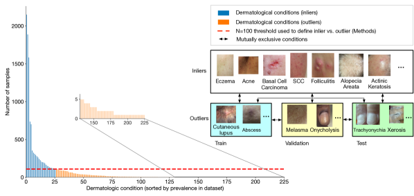
Classification of dermatological conditions through deep learning techniques is a typical clinical application where the long-tailed distribution of previously-unseen outliers poses a challenge (Prabhu et al., 2018). In previous work, Liu et al. (2020) demonstrated that a deep learning system could effectively distinguish among of the most common skin conditions. These represent around of cases in the tele-dermatology dataset used. The remaining of cases featured a long-tail distribution with hundreds of skin conditions that occurred considerably less frequently. This long-tailed distribution is illustrated in Fig. 1, with the common conditions indicated in blue and the rare ones in orange. Training models for classification of these rare conditions is prohibitively challenging due to the scarcity of available per-condition training examples.
Possible solutions include using class balancing techniques or few-shot learning approaches (Weng et al., 2020; Prabhu et al., 2018). However, Weng et al. (2020) showed that such approaches do not boost the performance on these rare conditions significantly, which suggests that these approaches cannot be deemed acceptable solutions for real-world deployment. Furthermore, the above solutions require the rare conditions to have been seen during training, whereas new unseen conditions may be encountered in real-world settings.
Another possible framing is to detect such rare conditions during test time - posing this challenge as an out-of-distribution (OOD) detection problem (Bulusu et al., 2020). Such approaches generally leverage model confidence for this purpose. It has been shown that deep learning models often produce over-confident predictions for OOD inputs (Goodfellow et al., 2014; Nguyen et al., 2015) suggesting that there remains room for improvement.
In this article, we aim to address the challenge of reliably detecting OOD rare dermatological conditions that were not seen during training. Most OOD detection works only use inlier samples during training (Hendrycks and Gimpel, 2017; Liang et al., 2018; Lakshminarayanan et al., 2017; Lee et al., 2018). In contrast, we have access to some ‘known outlier’ samples during training and we want to leverage them to aid detection of ‘unknown outlier’ samples during test time. This is similar to setup used in Hendrycks et al. (2019b); Thulasidasan et al. (2021), referred to as outlier exposure, which has shown to be more effective for OOD detection. Furthermore, most traditional OOD benchmarks in computer vision aim at detecting distribution shifts between datasets. Our task aims at detecting semantic shifts (difference in semantic information for images of two different classes) between conditions, referred to as the near-OOD detection problem (Winkens et al., 2020). This is more challenging as semantic distribution shifts are more subtle in comparison to dataset distribution shifts, and are thus harder to detect.
The key contributions of this article are:
-
1.
We propose a novel hierarchical outlier detection (HOD) loss, and show that this outperforms existing outlier exposure based techniques for detecting OOD inputs.
-
2.
We introduce a near-OOD benchmarking framework and the key design choices needed for proper validation of OOD detection algorithms.
-
3.
We demonstrated the added utility of the novel HOD loss in the context of multiple different state-of-the-art representation learning methods (self-supervised contrastive pre-training based SimCLR and MICLe). We also show the OOD detection performance gains on large scale standard benchmarks (ImageNet and BiT model pre-trained on a large-scale JFT dataset).
-
4.
We propose to use a diverse ensemble with different representation learning and objectives for improved OOD detection performance. We demonstrate its superiority over vanilla ensembles and performed analysis investigating how diversity aids in better OOD detection performance.
-
5.
We propose a cost-weighted evaluation metric for model trust analysis that incorporates the downstream clinical implications to aid assessment of real-world impact.
2 Related Work
In this section, we present an overview of relevant recent works in OOD detection and specifically applications to medical imaging and dermatology.
2.1 OOD Detection for Deep Learning
In the deep learning literature, the max-of-softmax probability (MSP) (Hendrycks and Gimpel, 2017) is a widely-used baseline method for OOD detection due to its simplicity and good performance. As the name suggests, MSP is defined as the maximum of the predictive class probabilities from the model. The method is based on the assumption that supervised training produces models that are less confident on OOD inputs. To enforce low confidence predictions for OOD data, one approach is to introduce a temperature hyper-parameter to the softmax layer to decrease the confidence of classification decisions. This hyper-parameter is tuned on the validation set containing outliers (Platt, 2000; Liang et al., 2018). Though in most applications, OOD data may not be available during training or validation, some medical applications are exceptions where some rare conditions may be available. To exploit such additional outlier data during training, methods such as Outlier Exposure (OE) (Hendrycks et al., 2019b) can be used. The key idea of OE is to include an extra term in the training objective for the OOD training data, additive to the regular cross entropy loss. This extra term forces a model to produce an output that is close to the uniform distribution for OOD samples such that the MSP score is lower. Hafner et al. (2019) propose a similar idea for regression tasks where they force the model’s predictive distribution for OOD data to be close to a prior uncertainty distribution by minimizing their KL divergence. Another common approach to utilize OOD training data is to add an extra, ’th OOD abstention class next to the inlier classes (Thulasidasan et al., 2021; Zhang and LeCun, 2017; Ren et al., 2019).
OOD detection is conceptually related to estimation of the confidence or uncertainty in classification decisions. Substantial improvement in uncertainty estimation is shown to be achieved using deep ensembles (Lakshminarayanan et al., 2017; Ovadia et al., 2019). Deep Ensembles involves training multiple models with randomly initialized network weights and with randomly shuffled training inputs. The MSP of the average predictive class probabilities over all models is used as an confidence score. Empirically, improvements over vanilla ensembling were achieved when models trained using different hyperparameter settings (such as learning rate schedules or weight decay) or different model architectures are combined within an ensemble (Wenzel et al., 2020; Kamnitsas et al., 2017). Though this method is known to enhance ensemble diversity and improve inlier prediction accuracy, its effect on OOD detection has not previously been explored.
More recent techniques such as pre-training, data augmentation, and self-supervised learning that enhance model robustness and generalization have also been shown to improve OOD detection performance (Hendrycks et al., 2020b, 2019a, a, c; Venkatakrishnan et al., 2020; Winkens et al., 2020). In particular, Winkens et al. (2020) show that using the contrastive self-supervised training technique, SimCLR (Chen et al., 2020), significantly helps near-OOD detection performance. Using a set of class-preserving transformations, SimCLR maximizes the similarity in learned embeddings between images that are transformed from the same original image, and minimize the similarity between images that are transformed from different images. This is thought to encourage the model to learn robust and invariant features which might lead to a better OOD detection.
In addition to MSP, another test statistic that is used for OOD detection is Mahalanobis distance based OOD scoring (Lee et al., 2018; Çallı et al., 2019). In contrast to network probability outputs, it leverages intermediate layer activations. A class conditional Gaussian distribution is fitted on the activations using training inlier data. The Mahalanobis distance between a test sample and the fitted distribution is used as an OOD score.
Another set of popular approaches is using generative models to directly fit inlier training data and use the likelihood of the test input as the OOD score. Several similar methods such as likelihood ratio (Ren et al., 2019), DoSE (Morningstar et al., 2021), variational autoencoders (Thiagarajan et al., 2020), and hybrid flows (Zhang et al., 2020) show promising performance on OOD detection but involve significant modifications to the training procedure and hyperparameter tuning.
There are several limitations to the existing methods discussed above. First, most of these generic OOD detection methods are evaluated using only standard benchmark datasets such as CIFAR-10, CIFAR-100, SVHN etc. While these approaches are viable for prototyping, they tend to require vast amounts of inlier training data and their OOD detection performance still needs careful evaluation in the context of each specific application, particularly for challenging settings such as medical imaging. Second, most of the methods with the exception of Hendrycks et al. (2019b) and Thulasidasan et al. (2021), do not use outlier data in the training process. In many real medical applications, some ‘known outlier’ samples are accessible. We believe incorporating them into the training process should help to improve the performance for detecting ‘unknown outliers’.
2.2 OOD Detection in Medical Imaging
Dealing with OOD inputs is a common problem that is faced across a broad spectrum of medical imaging applications. Recent studies have investigated this challenge for chest X-ray (Cao et al., 2020; Çallı et al., 2019; Shi et al., 2021), brain CT scans (Venkatakrishnan et al., 2020), fundus eye images (Cao et al., 2020) and histology images (Cao et al., 2020; Linmans et al., 2020). Due to the unique challenging properties of a long-tailed distribution comprising multiple conditions, OOD detection in the dermatology setting has drawn significant attention from the research community (Pacheco et al., 2020; Li et al., 2020; Combalia et al., 2020; Yasin et al., 2020; Thiagarajan et al., 2020). However, current studies have several limitations. Firstly, most of the studies for OOD detection in dermatology tackle dermatoscopic image classification on pigmented skin lesions using standard datasets such as the ISIC challenge dataset (Pacheco et al., 2020; Combalia et al., 2020; Li et al., 2020; Thiagarajan et al., 2020). Such studies can be limited in wider clinical utility, as images need to be acquired by a special device called dermatoscope, which are typically not available outside of dermatology clinics. In addition, only a handful of pigmented skin lesion conditions are addressed in these studies, whereas in real life hundreds or thousands more skin conditions such as rashes, hair loss, and nail conditions exist and may occur more frequently. Images in those datasets are also well-lit and magnified on the pathological region without background variability, making the classification and the OOD tasks relatively easy. Secondly, most of the existing methods either use different post-processing methods or complex density models. Pacheco et al. (2020) and Li et al. (2020) leverage feature maps from a pre-trained model for OOD detection. Thiagarajan et al. (2020) used a variational autoencoder to learn a disentangled latent representation to improve model interpretability and designed a calibration-driven learning approach to produce a prediction interval for uncertainty quantification. However, the method requires extensive modifications to the original classification model and very careful hyperparameter tuning. Thirdly, most of these methods focus mainly on the comparatively easy task of far-OOD detection: non-dermatology images or poor-quality images. A more challenging task is detecting previously unseen dermatological conditions, which is a near-OOD problem and remains relatively unexplored.
3 Benchmark Setup and Problem Formulation
3.1 Dataset Description
In this article, we use a subset of the de-identified dataset used in Liu et al. (2020) for model development. Cases in this dataset were collected from different sites across California and Hawaii. Each case in the dataset consists of up to RGB images, taken by medical assistants using consumer-grade digital cameras. The images exhibit a large amount of variation in terms of affected anatomic location, background objects, resolution, perspective and lighting. We resized each image to pixels for our training. The dataset consists of cases, with the ground truth generated by aggregating the diagnoses from multiple US or Indian board certified dermatologists. The detailed annotation process is presented in Liu et al. (2020). Note that for simplicity, we removed the cases that had multiple conditions or that had multiple primary diagnoses in the ground truth.
We use an additional unlabeled dermatology dataset consisting of images from cases and patients for contrastive training based representation learning outlined in Sec. 4.3 similar to Azizi et al. (2021). These images primarily come from skin cancer clinics in Australia and New Zealand, spread across different sites and Australian states. The distribution of conditions is skewed towards cancerous conditions but no labels were available for them.
3.2 Data Splitting Strategy
The long-tailed distribution of our dataset is illustrated in Fig. 1. Consistent with prior work (Liu et al., 2020), we select the most common conditions (based on primary diagnosis of each case, with number of cases with at least per condition) and consider them as inliers (indicated as blue). The remaining conditions (indicated in orange) are deemed as outliers. By definition the inlier and outlier conditions are mutually exclusive.
For setting up our OOD benchmark, we split this dataset into 3 sets: (i) train, (ii) validation and (iii) test. For each of the inlier conditions, we split the samples approximately in a split for the train-validation-test respectively. For the outlier conditions we also split the samples into train, validation and test such that outlier conditions assigned to each of these splits have mutually exclusive conditions as illustrated in Fig. 1. The full list of inlier and outlier conditions are detailed in Table 7. The splitting process satisfies the following desiderata:
-
1.
Patients do not overlap between the splits.
-
2.
Outlier conditions assigned across the splits are mutually exclusive.
-
3.
The number of outlier samples is similar across splits.
-
4.
The number of outlier conditions is similar across splits, ensuring that the outlier heterogeneity is similar across splits.
-
5.
Each outlier condition is associated with a worst-case risk level of clinical complications if left untreated (low, medium or high). We ensured a similar distribution of risk categories across the splits to enable downstream analyses on how the OOD detection methods perform across different risk levels.
-
6.
The distribution of cases with different Fitzpatrick skin types across the splits is similar to enable downstream analysis on how the OOD detection methods perform across different skin types.
These requirements can be generalized to establish a reliable benchmark for evaluating OOD methods for any dataset with a long-tailed distribution of classes. The statistics of the resulting splits for our work are detailed in Table 1. Note, real-world deployment may involve test outlier classes that were previously seen in training. Thus our more difficult setting of mutually exclusive conditions may underestimate the real-world performance of a OOD detection method.
| Train | Validation | Test | ||||
| Inlier | Outlier | Inlier | Outlier | Inlier | Outlier | |
| Num. classes | 26 | 68 | 26 | 66 | 26 | 65 |
| Num. samples | 8854 | 1111 | 1251 | 1082 | 1192 | 937 |
3.3 Problem Formulation
In this section, we provide a more formal definition of our problem statement, introducing the notations that will be used later in the paper. We denote the set of labels for all dermatological conditions in our dataset (such as ‘Eczema’, ‘Acne’ etc.; see Fig. 1) by . Total number of classes is denoted by . Let our long-tailed labeled dataset with cases be represented as . Here for indicates the sample input which corresponds to a set of image instances with and indicates its corresponding ground truth label with . Let indicate the required minimum sample size per condition for any condition to be considered as inlier. We fix similar to Liu et al. (2020) for all our experiments. Given , we split into two mutually exclusive inlier and outlier label sets as , where we formally define , essentially counting the number of instances that have the label in the dataset. is an indicator function. Consequently, . This also partitions the dataset naturally into two mutually disjoint sets , as an inlier and outlier dataset respectively.
We further split into , and . Similarly, we split into , and such that outlier conditions assigned to each of these splits are mutually exclusive as illustrated in Fig. 1 and detailed in Sec. 3.2. We denote these mutually exclusive set of outlier conditions by , and respectively. The train dataset is , validation dataset is and test dataset is . We train a deep neural network using and select our hyper-parameters using . The final task is to correctly distinguish from .
4 Methods
In this section, we describe the model architecture, the proposed hierarchical outlier detection loss and finally the various representation learning and model ensembling strategies we have investigated to boost OOD detection performance.
4.1 Architectural Details
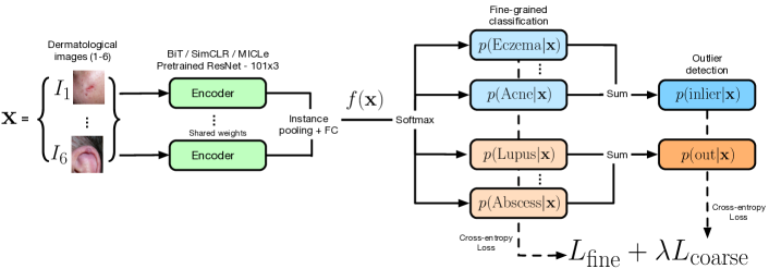
We illustrate the overall setup in Fig. 2. As detailed in the Sec. 3.3, we are dealing with a multi-instance dermatology image classification task. Specifically, each case contains image instances, and each case is assigned a primary diagnosis. We use a common encoder to process all the instances. A wide ResNet model is chosen as the encoder which is pre-trained with different representation learning approaches detailed later in Sec. 4.3. The encoder provides a feature representation for each image instance in a case. This output is then passed through an instance level average pooling layer, which generates a common feature-map for all the instances for a given case. This is passed to a classification head which has an intermediate fully-connected hidden layer with -dimensions followed by a final classification with a softmax layer which provide probabilities for each of the fine-grained inlier and train outlier classes. Note, we used ResNet- as the encoder architecture throughout for simplicity, though extensions to other architectures are straightforward.
4.2 Hierarchical Outlier Detection Loss
We build on the recent work by Thulasidasan et al. (2021) which proposed to have a dedicated abstention class, also referred to as a reject bucket for detecting OOD samples, trained using outlier data. This was shown to be effective in comparison to traditional entropy normalization-based outlier exposure method (Hendrycks et al., 2019b). The outlier samples used for training can have high variability in terms of semantics, acquisition source, resolution etc. Encapsulating such a heterogeneous outlier set within a single abstention class can be challenging. One natural mitigation strategy here is to assign multiple abstention classes as possible outputs, representing each of the individual outlier classes available at training via a fine-grained setup. In the dermatological setting, the approach of using multiple outlier classes is also practical as most often we have access to some labels associated with the training outlier data. Our setup is similar to this; we know the unique outlier classes within our training dataset even though the number of samples of some outlier classes can be as low as samples each. We conjecture that allowing multiple abstention classes has two main advantages: (i) it drastically reduces the burden of fitting a single highly heterogeneous class, hereby allowing a more structured decision boundary, (ii) it provides high capacity to properly model both the inlier and the outlier classes, resulting eventually in richer feature representations.
Clearly, with a better model for the training outliers, we ultimately want our network to generalize to test outlier samples that are not part of the fine-grained training outlier classes. This can be achieved by encouraging the model to learn features for a high-level semantic separation for the inlier vs. outlier classes. This can potentially assist in modeling the inlier samples by restricting the probability mass within the inlier classes rather than sharing with multiple outlier abstention classes and vice-versa.
Towards this end, we propose employing a Hierarchical Outlier Detection (HOD) loss. This is composed of a fine-grained low level loss and a coarse-grained high level loss. Given an input sample and its associated label from , let denote the output of the penultimate layer of our model. In our case is a vector of dimensions. The predictive probability for a class is expressed as
| (1) |
where and are the weights and bias of the last layer for class , and . Note that the network provides an output of dimension , with abstention classes.
The two level hierarchical loss is then constructed based on the predictive probabilities. The fine-grained loss is defined as the cross entropy loss, i.e. the negative log-likelihood, of the true label class ,
| (2) |
For the coarse-grained loss, we first define the probability of being an inlier as the sum of the probabilities of the fine-grained inlier classes in , . Similarly the probability of being an outlier is the sum of the probabilities of the fine-grained outlier classes in , . This is shown in Fig. 2. The coarse-grain level is a binary classification between classes . The coarse-grain loss is then defined as
| (3) |
As a training objective, we propose directly optimizing the following combined overall loss of
| (4) |
where the hyper-parameter dictates the relative importance of in comparison to . Fig. 2 illustrates the hierarchical loss structure. We define the OOD score and confidence scores as
| (5) | ||||
| (6) |
At test time, the individual probabilities for the abstention classes do not carry any importance because none of them show up in the test set. The sum of these probabilities indicating the OOD score is used.
We argue that the HOD loss provides two major benefits for OOD detection. First, the fine-grained loss is helpful for reducing OOD data heterogeneity per abstention class, hereby allowing more structured decision boundaries. Second, the coarse-grained loss plays a dynamic label smoothing role, improving the generalization for unseen outlier detection. In particular, for an OOD input where , the log-likelihood it contributes to is,
| (7) |
where the first term is for the fine-grained loss and the second is for the coarse-grained loss. To minimize the loss, equivalently maximizing the log-likelihood, the model can either through gradient descent increase , or increase the for the rest of the OOD classes. In other words, the fine-grained loss is to increase the probability for the particular class, and the coarse-grained loss is to increase the probability mass for the rest of the OOD classes. Even though that data point is for the OOD class , the parameters relevant to the rest of the OOD classes are also updated with respect to the gradient of this loss, leading to a similar effect as label smoothing. This property is extremely helpful when the test OOD classes are mutually exclusive from the training OOD classes. While the model is trained using training OOD classes, the test OOD data will not have high probability for any specific training OOD classes , as the test OOD class is unseen. But because of the coarse-grained loss, it may have relatively high probability in the aggregated probability for OOD classes , resulting in to a better generalization for OOD performance.
One interpretation of this combined loss is to think along the lines of data augmentation. Let us imagine that each input is associated with a coarse grained label and a fine-grained label. We duplicate this sample times and pair it with its fine-grained labels. Similarly, we duplicate the same sample times and pair them with its coarse labels. The combined log-likelihood contribution of the sample augmented times would be equivalent to our loss function , where .
Note that Yan et al. (2015) also incorporate the hierarchy among image classes into the model but in a different way: independent fine grained classification heads are constructed for each high level class. In addition, their study is for improving the inlier prediction accuracy, not for OOD detection. To the best of our knowledge, we are the first to use such a hierarchical loss for OOD detection.
4.3 Representation Learning
Representation learning has been proven effective for semi-supervised learning where the amount of training data is limited (Kolesnikov et al., 2019; Chen et al., 2020). While the main goal of representation learning is enabling label efficiency in downstream tasks, in this article, we will mainly explore the effectiveness of representation learning for downstream OOD detection task. We hypothesize that generic features may be learned during the pre-training phase. While these features may be discarded when training using only a supervised objective as they may not be directly useful for classification, we may be able to leverage these for OOD detection.
In image classification, a common representation learning approach is via a model pre-trained on ImageNet. We use a wide ResNet- feature extractor pre-trained on natural images from the ImageNet dataset as the baseline representation learning approach. An ImageNet based pre-training strategy was also used in Liu et al. (2020).
In addition, we explore two other representation approaches for our task: Big Transfer (BiT) as a supervised approach, and contrastive training as a self-supervised approach. These are detailed below.
4.3.1 Big Transfer (BiT) using JFT
Big Transfer (BiT) is a large scale supervised pre-training for visual representation learning, introduced by Kolesnikov et al. (2019). This was later extended to different medical applications and demonstrated promising results (Mustafa et al., 2021). The method provides a recipe for efficient transfer learning with minimal hyper-parameter tuning and its effectiveness is demonstrated in a plethora of vision tasks. The main architectural changes include: (i) using Group Normalization (Wu and He, 2018) instead of Batch Normalization and (ii) inclusion of weight standardization (Qiao et al., 2019), which aids effective transfer learning with variable batch size. In this paper, we use a wide ResNet- BiT model pre-trained on the large JFT dataset (Sun et al., 2017). This is referred as BiT-L. The purpose of this experimental choice is to investigate if adding considerably more natural images helps learn generic features to improve OOD detection compared to the ImageNet baseline.
4.3.2 Contrastive Training
We use two contrastive self-supervised learning methods for our application, which has been shown to be highly effective at representation learning (Chen et al., 2020). In contrast to ImageNet and BiT-L pre-training, we leverage unlabeled data from the target dermatology domain for pre-training our encoder optimizing the contrastive objective.
First, we use SimCLR (Chen et al., 2020) based contrastive pre-training due to its simplicity. SimCLR based pre-training has already been demonstrated to be effective on benchmark OOD tasks (Winkens et al., 2020) potentially due to the rich representations learnt. For our application we use SimCLR to pre-train a wide ResNet- model. This model was first pre-trained on ImageNet and then further trained on a set of unlabeled dermatology images using the contrastive objective. This includes images from both and from additional unlabeled dermatology dataset detailed in Sec. 3.1. The data augmentations used in this contrastive pre-training are random color augmentation, random crops ( pixels), Gaussian blur and random flips. Our hope is that using dermatological images for pre-training will aid learning of domain specific representations for downstream OOD detection.
Second, as our downstream classification task is multi-instanced in nature, we also use a multi-instanced version of contrastive training termed MICLe (Azizi et al., 2021). In contrast to SimCLR which tries to minimize the distance between two augmented versions of the same image, MICLe aims at minimizing the distance between two augmented image instances of the same case in the feature space. This modification help to learn representations that can distinguish each multi-instanced case from each other. The same unlabeled dermatology dataset as SimCLR was used for training.
We compare the OOD performance using ImageNet, BiT, SimCLR and MICLe representation learning, with HOD loss and with single reject bucket in the results.
4.4 Representational Diversity in Ensembles
We ensemble multiple models to further improve the OOD detection performance. For a set of ensemble members trained with random initialization and random shuffling of training inputs, we use the average of the predicted OOD score , as the final OOD score. Here indicates the OOD score for the model. If the model uses HOD loss, the OOD score is the sum of the probabilities of the fine-grained outlier classes in . If the model uses reject bucket loss, the OOD score is the probability of the reject bucket. For each of the proposed models, we choose because of diminishing returns beyond that (Lakshminarayanan et al., 2017).
Note that performance boost in deep ensembles depends on the model diversity introduced by random initialization of the network weights. In our setup, as we are using pre-trained models, random initialization is done only for the weights of the last layer. This reduces the diversity. To introduce more diversity, we also ensemble models trained with different representation learning and objective function to increase the diversity of the ensemble members. Given a set of candidate models, we use the greedy search algorithm proposed by Wenzel et al. (2020) to select the best subset of models whose ensemble gives the best OOD performance. In particular, we first collect all models we have trained using different representation learning and objectives: ImageNet initialized models with and without HOD loss, BiT models with and without HOD loss, SimCLR models with and without HOD loss and MICLe models with and without HOD loss. We greedily grow an ensemble, until reaching a fixed ensemble size, by selecting with replacement the model leading to the best improvement of OOD performance on the validation dataset. We refer to the selected ensemble as the diverse ensemble. We believe this diversity will boost OOD performance leveraging the complementary features learnt from the diverse representation learning approaches and objective functions we investigate. We compare the performance of this diverse ensemble with vanilla ensembles in the results.
5 Experimental Results
In this section, we present the experimental setup and the results of our experiments which includes ablation of the different components we propose and comparison to baseline approaches.
| Method | OOD detection metrics | |||
|---|---|---|---|---|
| AUROC () | FPR @ 0.95 TPR () | AUPR-in () | Inlier accuracy () | |
| BiT-L + MSP⋆ | ||||
| BiT-L + Mahalanobis⋆ | ||||
| BiT-L + Outlier exposure + MSP | ||||
| BiT-L with reject bucket | ||||
| BiT-L with fine-grained outlier () | ||||
| BiT-L + HOD () | ||||
| BiT-L + HOD () | ||||
| BiT-L + HOD () | ||||
5.1 Experimental Settings and Evaluation Metrics
Here we detail the experimental setting for all the models and introduce the evaluation metrics we use for comparing different methods.
Experimental settings
We use the train split (as detailed in Table 1) for training all the models. We use data augmentation for training. This includes: random horizontal and vertical flips, random variations of brightness (max intensity = ), contrast (intensity = []), saturation (intensity = []) and hue (max intensity = ), random Gaussian blurring using standard deviation between and and random rotations between and . We use a Stochastic Gradient Descent optimizer with momentum with exponentially decaying learning rate for training. Each model is trained for steps. Convergence of all the models were ensured on the validation set. We use a batch-size of cases for training. We use the validation split to set the hyper-parameters (e.g. initial learning rate, decay factor, momentum) and to select the best checkpoints for all the models. Checkpoint selection was based on the OOD Area under Receiver Operating Characteristic Curve (AUROC). AUROC provides a quantitative measure of predictive performance for outliers using the OOD score, with higher values indicating higher power in discriminating inliers and outliers using the OOD score. We report all the results in the following sections on all the samples in the held out test split . Note that all the metrics used for evaluation do not require selection of a fixed operating point.
Evaluation metrics
For evaluating the OOD performance for different methods, we use 3 commonly used metrics: (i) AUROC (higher is better), (ii) False positive rate at true positive rate (FPR TPR, lower is better) and (iii) Area under inlier precision-recall curve (AUPR-in, higher is better). Along with the OOD metrics, we also track the inlier accuracy of the models to investigate any possible trade-off between accuracy and OOD performance of the models. The inlier accuracy is computed only on the test inlier set, comparing the ground-truth to the top-1 inlier prediction.
5.2 Comparison of HOD Loss with Existing Methods
In this section we compare our proposed HOD loss with existing methods and ablation of the different parts of the HOD loss. As an architectural backbone for this ablation we choose the BiT-L initialized wide ResNet . First we investigate the most commonly used OOD detection methods: MSP (Hendrycks and Gimpel, 2017) and Mahalanobis distance (Lee et al., 2018). Note that these baselines do not use outlier samples in the training process. We present the results in the first two rows of Table 2. We observe that MSP baseline outperforms Mahalanobis baseline by AUROC points. Next, we investigate existing methods which use training outliers: outlier exposure (OE) with MSP (Hendrycks et al., 2019b) and reject bucket (Thulasidasan et al., 2021). We present the results in Table 2. We observe that OE with MSP outperforms the MSP baseline by AUROC points. The reject bucket baseline further outperforms OE by AUROC points. It is clear from the results that methods using outliers during training are better than the methods not using them. Among all the existing methods the reject bucket method has the best OOD detection performance and we use it for comparison for the next experiments.
Note that the reject bucket based baseline uses a single abstention class to encapsulate the OOD data (Thulasidasan et al., 2021). As illustrated in Sec. 4.2 HOD introduces two modifications on top of this: (i) expanding the reject bucket into fine-grained training outlier classes, and (ii) inclusion of a coarse loss term along with fine-grained loss. We also explored different choices of which dictates the relative contribution of fine-grained and coarse-grained loss terms. We present the results for all the settings on the test set in Tab. 2.
| Method | OOD detection metrics | |||
|---|---|---|---|---|
| AUROC () | FPR @ 0.95 TPR () | AUPR-in () | Inlier accuracy () | |
| ImageNet + reject bucket | ||||
| ImageNet + HOD | ||||
| BiT-L + reject bucket | ||||
| BiT-L + HOD | ||||
| SimCLR + reject bucket | ||||
| SimCLR + HOD | ||||
| MICLe + reject bucket | ||||
| MICLe + HOD | ||||
First we observe that expanding the abstention class to fine-grained outlier classes improves OOD detection AUROC by points and inlier accuracy by points compared to reject bucket baseline. This indicates that assigning multiple class-specific buckets to outlier samples is better than encapsulating all highly heterogeneous outlier samples in a single abstention class both for OOD detection and inlier accuracy. Inclusion of a coarse loss with further boosts performance by point AUROC with a slight decrease of points accuracy compared to having multiple abstention classes i.e. . The inclusion of the coarse loss had a large impact in reducing FPR TPR by points which was not observed with .
Also, we observe that assigning higher weights to the coarse loss drastically degrades both the inlier accuracy and OOD detection performance. We believe this is due to the strong label smoothing regularizing effect that the coarse loss provides. Setting a very high is similar to training a model for a binary inlier/outlier classification only. Note that inlier accuracy drops drastically with higher values of . Thus, we fix the value of to and use this setting for the following experiments.
Note that Mahalanobis method (Lee et al., 2018) can also be used as an OOD score. This involves fitting class conditional Gaussians for the inliers in the high-dimensional feature space and use the Mahalanobis distance for a test sample to the fitted distribution as an OOD score. We performed experiments using the dimensional . We observed that it consistently performed poorly compared to using as an OOD score. For BiT-L with reject bucket, on the validation set had an AUROC of , whereas the Mahalanobis method had an AUROC of . We believe this drop is due to the under-fitting of the Gaussians in the feature space. Fitting a Gaussian in a dimensional space requires estimating parameters for the mean vector and co-variance matrix. Note that for our application, we also have a class imbalance among the inlier conditions (see Fig. 1). The sample count for some inlier classes is not sufficient for reliably fitting a high-dimensional Gaussian in the feature space. The Mahalanobis method works well in most public benchmarks as they have a balanced inlier class distribution. Thus, we only use as the OOD score in this work.
5.3 Effect of Different Representation Learning Methods
In this section we investigate how different types of representation learning (see Sec. 4) helps in OOD detection in conjunction with HOD: ImageNet pre-trained, BiT-L pre-trained, SimCLR pre-trained and MICLe pre-trained models. First, as shown in Table 3, we observe that including HOD loss improves OOD performance compared to reject bucket for all the four representation learning methods. The AUROC increases by points, points, points and points for ImageNet, BiT-L, SimCLR and MICLe pre-trained models respectively. The boost is much higher in BiT-L in comparison to others. HOD also boosts the inlier accuracy for BiT-L checkpoints by 1.2 points. However, we observed a drop in inlier accuracy by , and points with HOD for ImageNet, SimCLR and MICLe respectively. Note that after training the model checkpoint was selected based on best AUROC performance on validation split. For ImageNet, SimCLR and MICLe with HOD loss, inlier accuracy and AUROC peaks at different stages of the training and there seems to be a trade-off between the two. This might be a possible reason for this drop in inlier accuracy.
Comparing the natural image based pre-training methods (ImageNet, BiT-L), we observe that BiT-L has a better inlier accuracy and OOD performance. We can conclude that using much larger-scale datasets (JFT) for pre-training helps not only for better classification performance but also for better OOD detection task. Comparing the contrastive training based methods (SimCLR, MICLe), we observe that although MICLe and SimCLR yields similar inlier accuracy, OOD performance of MICLe is much better than SimCLR. SimCLR based pre-training learns to distinguish every image and does not consider the multi-instance aspect of our task. By considering the multi-instance aspect, MICLe may have learned case-specific features that are more useful for detecting case-level OOD samples.
Comparing the reject bucket based models, we also observe that contrastive learning based models have higher inlier accuracy in comparison to natural image based representation learning ones. We believe this is due to the additional unlabeled dermatology images used for contrastive learning which aided in learning domain specific features. This played a major role only for models with reject bucket.
| Method | OOD detection metrics | |||
|---|---|---|---|---|
| AUROC () | FPR @ 0.95 TPR () | AUPR-in () | Inlier accuracy () | |
| ImageNet + reject bucket + Ensemble | ||||
| ImageNet + HOD + Ensemble | ||||
| BiT-L + reject bucket + Ensemble | ||||
| BiT-L + HOD + Ensemble | ||||
| SimCLR + reject bucket + Ensemble. | ||||
| SimCLR + HOD + Ensemble | ||||
| MICLe + reject bucket + Ensemble | ||||
| MICLe + HOD + Ensemble | ||||
| Diverse ensemble | ||||
5.4 Comparison of Ensembling Strategies
In this section, we study different ensembling strategies and investigate their efficacy for OOD detection. For this study, we use all the different representation learning methods detailed in Sec. 5.3, with reject bucket and with HOD loss. Firstly, we investigate the vanilla ensembling strategy. For each of the methods, we ensemble five models trained independently with random initialization and random data shuffling. Note that as we used pretrained models for initialization, only the final fully connected layer and classifier layer weights were randomly initialized. Table 4 shows the performance of each method after ensembling. Compared with Table 3, it is clear that for every method, ensembling improves both inlier accuracy and OOD detection performance in comparison to their single-model counter-parts.
Secondly, we investigate ensembling models with different representation learning methods as described in Sec. 4.4. For the purposes of testing the diverse ensemble strategy, we pool together all the models for ImageNet, BiT-L, SimCLR and MICLe with reject bucket and with HOD and employ a greedy search algorithm (Wenzel et al., 2020) to select a set of models. The selection criteria metric for the greedy search algorithm was the mean of all 3 OOD metrics: AUROC, FPR TPR and AUPR-in. The ensemble with the highest validation set performance was selected for use (Table 4). The selected five models are three BiT-L pre-trained models with HOD loss and two MICLe pre-trained models with HOD loss. This diverse ensemble achieves the highest AUROC of , AUPR of , inlier accuracy of , and the lowest FPR TPR of . The diverse ensemble selected only HOD loss based models, indicating they were stronger candidates than the reject bucket based models. Further, note that the greedy search algorithm selects models from from two different representation learning (BiT and MICLe). We believe natural image based pre-trained BiT-L and contrastive learning based pre-trained MICLe models learn complementary features. Training with natural images may have helped by learning more generic low level features, whereas contrastive learning may have helped in learning more dermatology-specific features during its pre-training phase. This promotes learning both high-level and low-level features which might not be very useful for inlier classification, but might be useful for identifying previously unseen OOD examples. This complimentary nature may have enhanced the diversity during the selection process. Furthermore, note that the drop in inlier accuracy performance of the HOD loss in MICLe models for vanilla ensembles is compensated by the diverse ensemble. We use this diverse ensemble model as our final model for the subsequent analysis.
6 Discussion
As the final model is determined, in this section we discuss a few factors that may provide useful guidance for further improvement. We also perform downstream analysis of the model’s performance for different subgroups of risk levels and skin types, and we perform a trust analysis to better understand the model’s total clinical implications.
| AUROC | |||
|---|---|---|---|
| classes | samples | () | |
| BiT-L + MSP | |||
| BiT-L + HOD-17 | |||
| BiT-L + HOD-34 | |||
| BiT-L + HOD-51 | |||
| BiT-L + HOD-68 |
6.1 Available Training Outlier Data
In this section, we investigate the OOD performance of the model with varying amounts of training outlier data. We hypothesize that both quantity (number of train outlier samples) and quality (number of outlier train classes) play a major role in efficiently detecting outliers during deployment. To investigate this we use different proportions of training outlier data to train models and presented the results in Table 5. We use the BiT-L with HOD loss for this experiment. For each setting, we train different models and report the mean and standard deviation of OOD detection AUROC. We use the same validation set for checkpoint selection and hyper-parameter tuning and reported results on the same test set for all settings.
As a first setup, we show the results of not using any outliers during training. For this we trained a BiT-L pre-trained model only with inlier samples and used max-of-softmax (MSP) probabilities as the OOD score (Hendrycks and Gimpel, 2017). We indicate this as BiT-L + MSP in Table 5. Following that we uniformly increase more training outlier classes and samples. Each entry is indicated by BiT-L + HOD-xx, where xx corresponds to number of training outlier class i.e. number of abstention classes used in training. The last row includes the entirety of our training outlier set with outlier classes as indicated in Table 1. We observe that as we increase the training outlier heterogeneity and quantity the OOD detection performance increases consistently. Given the lack of plateauing, introducing additional training outlier classes and samples may potentially increase OOD detection performance further.
6.2 Diversity in ensembles
In Sec. 5.4, we demonstrated that diverse ensemble selected by a greedy search algorithm outperforms all the vanilla ensemble models. In this section, we investigate how diversity plays a role in achieving this performance boost. In our pool of models we have diversity in the following aspects: (i) representational diversity (pre-training strategies with ImageNet, BiT-L, SimCLR and MICLe), (ii) diversity in objective function (two different losses: reject bucket loss and HOD loss) and (iii) diversity due to last layer initialization and random input shuffling (vanilla ensembling).
To quantify diversity between any two models and , we use the average predictive disagreement between them similar to (Fort et al., 2019). For each input sample , let the top-1 predicted class given by be and by be . The diversity is given as
| (8) |
where indicates the expectation operator. Note that for computing top-1 prediction we perform an over the output class probabilities, which includes all the fine-grained inlier conditions and a single outlier class given by .
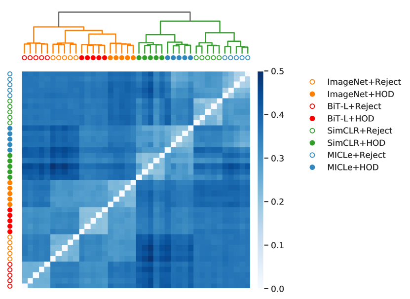
In Fig. 3(a), we present a diversity heatmap for all the models in our pool. The darker shades indicate higher diversity and the lighter shades indicates low diversity. Using the diversity in Eqn. 8 as the pair-wise distance between models, we apply hierarchical clustering using Ward’s minimum variance, over the pool of models and show the corresponding dendrogram at the top of Fig. 3(a). At the highest level of the dendrogram, we observe a separation between all contrastive pre-trained (SimCLR, MICLe) models and natural image pre-trained (ImageNet, BiT-L) models. This indicates that different representation learning provides the most diversity within our pool. At the middle level, we observe a separation between the models trained with reject bucket loss and HOD loss. This indicates that the difference in objective function provides the second most diversity. At the lowest level, we observe all the vanilla ensemble models with same representation learning and loss function are clustered together. It is visible as 8 block matrices of size along the diagonal of the heat matrix with lighter shades. This indicates that the diversity is minimum among them.
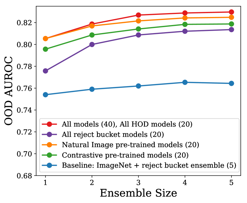
As detailed in Sec. 4.4, we employ a greedy search algorithm over the pool of models to select our diverse ensemble members. The greedy search algorithm aims to select an ensemble member which provides the highest performance boost at every step. This boost can be achieved by leveraging the diversity among the models using their complementary performance. We believe that the selected diverse ensemble depends on the diversity of the pool of models. To investigate this we employ the greedy search algorithm on different pools of models and plot the OOD AUROC for them at varying ensemble sizes in Fig. 3(b). The sub-pools were generated by the main diversity factors i.e. representation learning and objective function as observed in Fig. 3(a). As a baseline we present the performance of the ImageNet pre-trained models with reject bucket (blue, pool size: 5). We show the performance over pool of all models trained with reject bucket loss (purple, pool size: 20), pool of all models trained with HOD loss (red, pool size: 20), pool of all models pre-trained with contrastive learning (green, pool size: 20), pool of all models pre-trained with natural images (orange, pool size: 20) and overall pool (red, pool size: 40). Identical models were selected over all the models and over all the models with HOD loss, and we observe this set of selected model to perform the best. The selected diverse ensemble over pool of models pre-trained with natural images are better than the ones selected over the pool of contrastive pre-trained models at every ensemble size. The diverse ensemble selected over models trained with reject bucket under-performs compared to the others.
Along with the selected ensemble members, it is also interesting to observe the order in which the greedy search algorithm selects them at every step. For example, the final diverse ensemble over all models has 3 BiT-L + HOD models and 2 MICLe + HOD models. The sequence in which they were added to diverse ensemble is: BiT-L-HOD MiCLe-HOD BiT-L-HOD MiCLe-HOD BiT-L-HOD. Note the alternate addition of BiT-L and MICLe models. This indicates that the greedy search algorithm attains the maximum boost in performance at every step by balancing the representational diversity of the models. The above results also suggest that introducing additional representation learning strategies and loss functions can further enrich the model pool diversity, and may lead to better OOD performance.
6.3 Subgroup Analysis of OOD Detection Performance
In this section, we investigate how our final diverse ensemble model performs across different skin condition risk categories and skin type subgroups. As a baseline model, we compare against a vanilla ensemble of ImageNet pre-trained models, trained with a reject bucket similar to Liu et al. (2020).
| Subgroups | Num. Inlier | Num. Outlier | Baseline ensemble | Diverse ensemble |
|---|---|---|---|---|
| samples | samples | AUROC () | AUROC () | |
| High Risk | ||||
| Medium Risk | ||||
| Low Risk | ||||
| Skin-types-1&2 | ||||
| Skin-types-3 | ||||
| Skin-types-4 | ||||
| Skin-types-5&6 |
6.3.1 Analysis Over Risk Subgroups
For this purpose, dermatologists labeled each of the outlier classes in the test set as one of the three risk categories. Low risk indicates conditions that may cause either no injury or only temporary discomfort; medium risk indicates conditions that can result in injury or impairment requiring medical intervention to prevent permanent impairment; high risk indicates conditions that can result in permanent impairment or life threatening injury or death. All risk category assignments are based on the worse case scenario if left untreated; for example, though conditions like ‘Urticaria’ have a small chance to cause death, they are assigned to the high risk category. We present the results of this subgroup analysis on the test set in Table 6. Each AUROC value compares the inliers vs. outliers of subgroup X. We observe that our diverse ensemble has a higher AUROC than the baseline ensemble by 7.6, 2.5 and 8.2 points for high-risk, medium-risk and low-risk subgroups, respectively. The most substantial gains are for the high-risk and low-risk subgroups.
6.3.2 Analysis Over Skin Type Subgroups
For this analysis we divide the test set samples based on Fitzpatrick skin types. We analyzed 4 subgroups: (i) Types-1&2 (Pale-white and white skin), (ii) Type-3 (Beige skin), (iii) Type-4 (Brown skin) and (iv) Types-5&6 (Dark brown and black skin). The objective of this analysis differs slightly from the risk subgroups. Instead of stratifying based on the category of skin condition (which a user may not know), here we analyze subgroups based on information that a user may know: their skin type. For this purpose we computed our AUROC metric comparing inliers of subgroup X vs. outliers of subgroup X. We present the results on the test set in Table 6. Note that out of the test samples, we had access to ground-truth skin types for samples. In general we observe that our diverse ensemble had a higher AUROC for all 4 subgroups. The margin of 17 points AUROC for Types-5&6 is particularly striking as these skin types were rare in our dataset, though the smaller sample size render making confident conclusions difficult.

6.4 Qualitative Analysis and Failure Cases
In this section, we perform a qualitative analysis of our results and show the failure cases. For this purpose, we compare our diverse ensemble with the baseline ensemble similar to Sec. 6.3. First we show a scatter plot (Fig. 4a) of all the test outlier samples (in orange) and the inliner samples (in blue as a density plot in Fig. 4a) comparing the OOD scores assigned by the baseline ensemble versus the diverse ensemble. The outlier samples in the bottom-left region where inlier density is high corresponds to the difficult cases where both our model and baseline model fails. We select two cases from this category (indicated by red circle) and show them in Fig. 4b (outlined in red box). The top-left region in Fig. 4a represents the cases where baseline is better than our model. We select one such case (indicated by green circle) and show that in Fig. 4b (outlined by green box). The bottom-right region in Fig. 4 represents the cases where our model outperformed the baseline model. We randomly select two cases from this region (indicated by blue circle in Fig. 4a) and show them in Fig. 4b (outlined by blue box). The top-right region in Fig. 4a represents the cases where both the baseline and our models performed well. These mostly corresponds to relatively easy cases.
In Fig. 4a, we also show the marginal distributions of inliers (indicated in blue) and outliers (indicated in orange) modelled by baseline ensemble (right) and by our diverse ensemble (top). We can observe that the inlier distribution modelled by our diverse ensemble is more compact and narrower in comparison to the baseline ensemble. Also, we observe substantially more overlap between the inlier and outlier distributions for the baseline in comparison to our model. This provides qualitative evidence of our model being better at detecting outliers in comparison to the baseline.
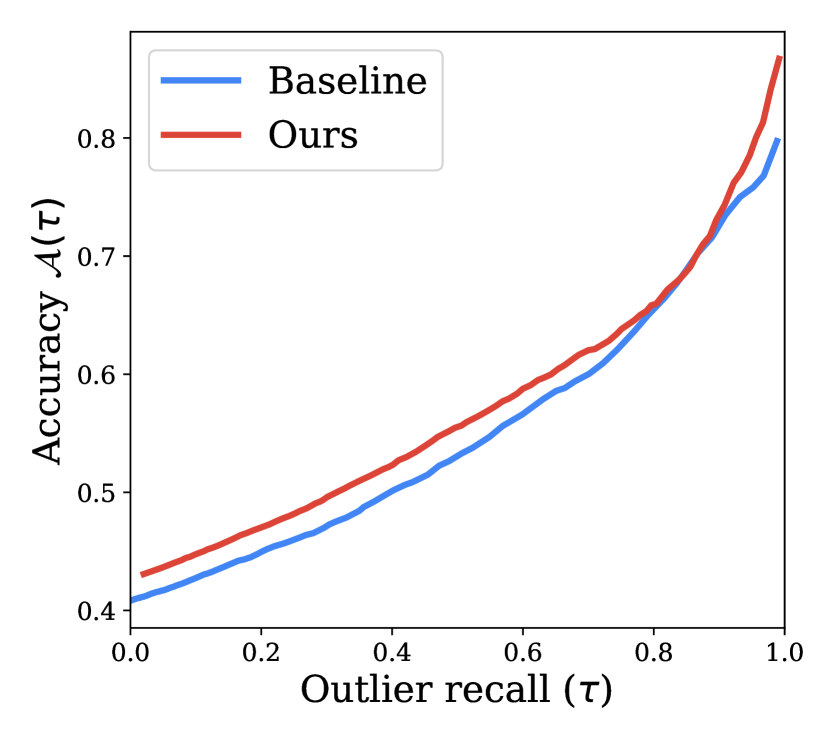
6.5 Joint Evaluation for Inliers and Outliers Predictions
Although in this article we mainly focus on improving the performance for OOD detection, the ultimate goal for our dermatology model is to have a high detection accuracy for both inliers and outliers. Therefore, in this section we investigate the model’s joint prediction accuracy for inliers and outliers.
Let us consider a confidence score threshold above which we allow our model to predict, i.e. if the test samples has a confidence scores its associated output will be predicted and if we abstain from prediction. For a fixed , corresponding model accuracy ) for the predicted samples can be computed as
| (9) |
which evaluates the inlier accuracy for the predicted samples, and considers all predictions for outliers incorrect.
Note that there is a calibration difference between our diverse ensemble model and the baseline ensemble model. Thus the of diverse ensemble and baseline ensemble for a fixed is not directly comparable. Thus to normalize the confidence threshold , we compute the outlier recall for the value of , which adjusts for the differences in calibration of the models.
We evaluate the and outlier recall at different thresholds and plot them in Fig. 5(a) similar to Lakshminarayanan et al. (2017); Van Amersfoort et al. (2020). We observe that our diverse ensemble model has higher accuracy than the baseline ensemble model for all outlier recall rates. This indicates that our model is better at jointly identifying outliers and correct inliers in contrast to baseline for different choices of operating points.
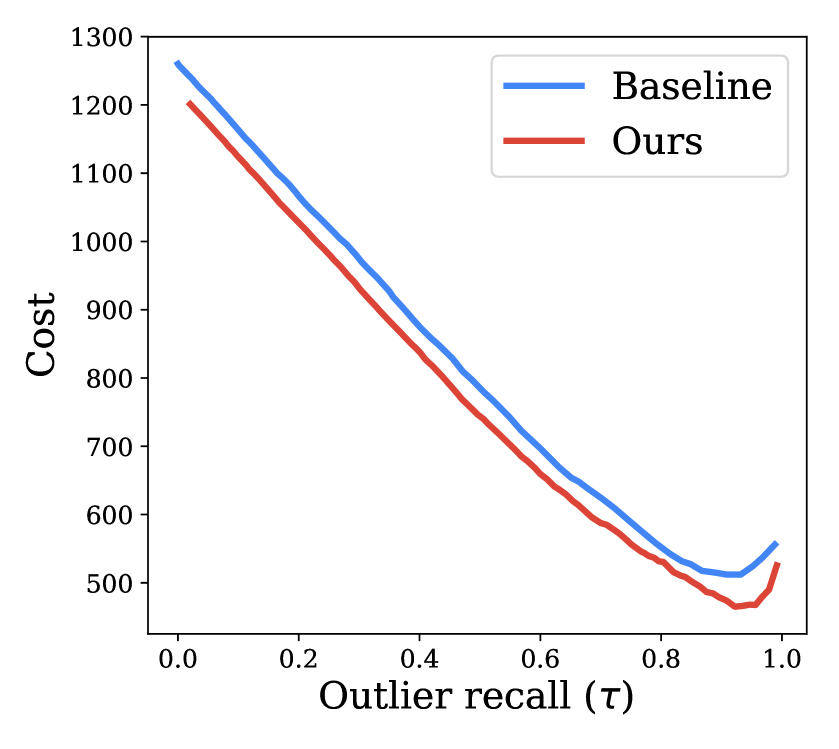
6.6 Model Trust Analysis
In this section, we perform a model trust analysis to better understand the total downstream clinical implications of the model for misclassifying inliers and outliers. For a fixed confidence threshold , we count the following types of mistakes: (i) incorrect prediction for inliers (i.e. mistaking inlier condition A as inlier condition B), (ii) incorrect abstention of inliers (i.e. abstaining from making a prediction for a inlier), (iii) incorrect prediction for outliers as one of the inlier classes. In order to account for the asymmetric clinical consequences of these different types of mistakes, we present a cost matrix assigning different costs for the different mistakes in Fig. 6. Both within-inlier incorrect predictions and outlier-as-inlier were penalized with a score of . Such mistakes can potentially erode trust of the user in the model.
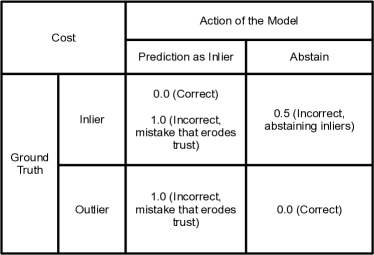
Incorrect abstention of inliers as an outlier was penalized with a score of to reflect the fact that potential users of the model would be able to seek additional guidance given the model-expressed uncertainty or abstention. Note that these numbers are qualitative approximations for modeling the downstream impact. Real-world scenarios are more complex and contain a variety of unknown variables; this has been simplified to better understand the main focus of this work: outlier detection and inlier accuracy. These choices were verified by a dermatologist.
We estimate the cost for both our diverse ensemble model and baseline ensemble model at different values of confidence thresholds and show the plot in Fig. 5(b). Similar to the accuracy, we use outlier recall at different to adjust for the different calibrations of the in the two models. We observe that our diverse ensemble model has lower overall cost than the baseline ensemble model across all outlier recall rates, and the lowest cost is achieved at the outlier recall rate . The consistently lower cost indicates our model performs better after accounting for different downstream clinical implications.
7 Conclusion
In real-world deployment of medical machine learning models, test inputs with previously unseen conditions are often encountered. For safety it may be important to identify such inputs and abstain from classification, in order to guard against inappropriate over-reliance on model outputs and empower model users to pursue safe next steps such as consulting a clinician.
In this article, we tackle this challenging task of detecting the previously unseen long-tail of rare conditions for a dermatology classification model. We frame this task as an out-of-distribution (OOD) detection problem. Leveraging our labeled dataset with a long-tail of conditions, we first construct a benchmark for reliably evaluating OOD methods.
We further propose a novel hierarchical outlier detection (HOD) loss function for OOD detection. In contrast to existing approaches of assigning a single abstention class for OOD, we assign multiple abstention classes corresponding to the number of OOD classes available in the train set. Also, in addition to the fine-grained classification loss, we include a coarse loss to aid high level clustering of inliers and outliers. We demonstrate the additional performance gains from using HOD loss compared to using baselines.
We additionally explore the utility of the HOD loss in the context of multiple different state-of-the-art representation learning methods. Beyond the commonly used ImageNet pre-trained model, we investigate the BiT model pre-trained on large-scale JFT dataset, and contrastive pre-training based SimCLR and MICLe approaches. We demonstrated that better representation learning can improve OOD detection performance, and that these can also be improved via the HOD loss.
We also explored different ensembling strategies. A vanilla ensemble improved both the OOD performance and inlier accuracy for all the models trained with and without HOD loss and different representation learning techniques. The diverse ensemble selection approach using a greedy search algorithm on a pool of models with different representation learning and loss functions further outperformed the vanilla ensemble models both for OOD performance and inlier accuracy.
We also investigated the OOD performance for different subgroups of risk levels and skin types. We show that our proposed method demonstrated superior performance in comparison to the baseline for all the subgroups.
To quantify potential downstream clinical implications, we go beyond the traditional performance metrics and construct a cost matrix for model trust analysis. We demonstrate the superiority of our method over baseline in this metric, indicating the effectiveness of our model for real-world deployment. Ideally we may directly optimize for this cost matrix as an objective function during training. We leave this as a possible future work.
All in all, we believe that our proposed approach can aid successful translation of AI algorithms into real-world scenarios. Although we have primarily focused on OOD detection for dermatology, most of our contributions are fairly generic and can be easily to generalized to OOD detection in other applications.
Acknowledgements
We would like to thank Olaf Ronneberger, Ali Eslami, Rudy Bunel, Simon Kohl, Krishnamurthy Dvijotham from DeepMind, Jonathan Deaton from Google Health and Neil Houlsby from Google Research for helpful discussions towards initial ideation. We would also like to express our appreciation towards Joshua Dillon, Jasper Snoek, Jeremiah Liu from Google Research, and Atilla Kiraly, Terry Spitz, and Dale Webster from Google Health, and Kimberly Kanada for insightful discussion and providing valuable feedback for this work, and Jay Hartford from Google Health for assistance in data-related logistics.
References
- Azizi et al. (2021) Azizi, S., Mustafa, B., Ryan, F., Beaver, Z., Freyberg, J., Deaton, J., Loh, A., Karthikesalingam, A., Kornblith, S., Chen, T., et al., 2021. Big self-supervised models advance medical image classification. arXiv preprint arXiv:2101.05224 .
- Bulusu et al. (2020) Bulusu, S., Kailkhura, B., Li, B., Varshney, P.K., Song, D., 2020. Anomalous example detection in deep learning: A survey. IEEE Access 8, 132330–132347. doi:10.1109/ACCESS.2020.3010274.
- Çallı et al. (2019) Çallı, E., Murphy, K., Sogancioglu, E., Van Ginneken, B., 2019. Frodo: Free rejection of out-of-distribution samples: application to chest x-ray analysis. arXiv preprint arXiv:1907.01253 .
- Cao et al. (2020) Cao, T., Huang, C., Hui, D.Y.T., Cohen, J.P., 2020. A benchmark of medical out of distribution detection. arXiv preprint arXiv:2007.04250 .
- Chen et al. (2020) Chen, T., Kornblith, S., Norouzi, M., Hinton, G., 2020. A simple framework for contrastive learning of visual representations. International conference on machine learning , 1597–1607.
- Combalia et al. (2020) Combalia, M., Hueto, F., Puig, S., Malvehy, J., Vilaplana, V., 2020. Uncertainty estimation in deep neural networks for dermoscopic image classification. Proceedings of the IEEE/CVF Conference on Computer Vision and Pattern Recognition Workshops , 744–745.
- Fort et al. (2019) Fort, S., Hu, H., Lakshminarayanan, B., 2019. Deep ensembles: A loss landscape perspective. arXiv preprint arXiv:1912.02757 .
- Goodfellow et al. (2014) Goodfellow, I.J., Shlens, J., Szegedy, C., 2014. Explaining and harnessing adversarial examples. arXiv preprint arXiv:1412.6572 .
- Hafner et al. (2019) Hafner, D., Tran, D., Lillicrap, T., Irpan, A., Davidson, J., 2019. Noise contrastive priors for functional uncertainty. Uncertainty in Artificial Intelligence , 905–914.
- Hendrycks et al. (2020a) Hendrycks, D., Basart, S., Mu, N., Kadavath, S., Wang, F., Dorundo, E., Desai, R., Zhu, T., Parajuli, S., Guo, M., et al., 2020a. The many faces of robustness: A critical analysis of out-of-distribution generalization. arXiv preprint arXiv:2006.16241 .
- Hendrycks and Gimpel (2017) Hendrycks, D., Gimpel, K., 2017. A baseline for detecting misclassified and out-of-distribution examples in neural networks. ICLR .
- Hendrycks et al. (2019a) Hendrycks, D., Lee, K., Mazeika, M., 2019a. Using pre-training can improve model robustness and uncertainty. International Conference on Machine Learning , 2712–2721.
- Hendrycks et al. (2020b) Hendrycks, D., Liu, X., Wallace, E., Dziedzic, A., Krishnan, R., Song, D., 2020b. Pretrained transformers improve out-of-distribution robustness. arXiv preprint arXiv:2004.06100 .
- Hendrycks et al. (2019b) Hendrycks, D., Mazeika, M., Dietterich, T., 2019b. Deep anomaly detection with outlier exposure. ICLR .
- Hendrycks et al. (2020c) Hendrycks, D., Mu, N., Cubuk, E.D., Zoph, B., Gilmer, J., Lakshminarayanan, B., 2020c. Augmix: A simple data processing method to improve robustness and uncertainty. ICLR .
- Kamnitsas et al. (2017) Kamnitsas, K., Bai, W., Ferrante, E., McDonagh, S., Sinclair, M., Pawlowski, N., Rajchl, M., Lee, M., Kainz, B., Rueckert, D., et al., 2017. Ensembles of multiple models and architectures for robust brain tumour segmentation. International MICCAI brainlesion workshop , 450–462.
- Kolesnikov et al. (2019) Kolesnikov, A., Beyer, L., Zhai, X., Puigcerver, J., Yung, J., Gelly, S., Houlsby, N., 2019. Big transfer (bit): General visual representation learning. preprint arXiv:1912.11370 .
- Lakshminarayanan et al. (2017) Lakshminarayanan, B., Pritzel, A., Blundell, C., 2017. Simple and scalable predictive uncertainty estimation using deep ensembles. NeurIPS .
- Lee et al. (2018) Lee, K., Lee, K., Lee, H., Shin, J., 2018. A simple unified framework for detecting out-of-distribution samples and adversarial attacks. arXiv preprint arXiv:1807.03888 .
- Li et al. (2020) Li, X., Lu, Y., Desrosiers, C., Liu, X., 2020. Out-of-distribution detection for skin lesion images with deep isolation forest. International Workshop on Machine Learning in Medical Imaging , 91–100.
- Liang et al. (2018) Liang, S., Li, Y., Srikant, R., 2018. Enhancing the reliability of out-of-distribution image detection in neural networks. ICLR .
- Linmans et al. (2020) Linmans, J., van der Laak, J., Litjens, G., 2020. Efficient out-of-distribution detection in digital pathology using multi-head convolutional neural networks. Proceedings of Machine Learning Research .
- Liu et al. (2019) Liu, X., Faes, L., Kale, A.U., Wagner, S.K., Fu, D.J., Bruynseels, A., Mahendiran, T., Moraes, G., Shamdas, M., Kern, C., et al., 2019. A comparison of deep learning performance against health-care professionals in detecting diseases from medical imaging: a systematic review and meta-analysis. The lancet digital health 1, e271–e297.
- Liu et al. (2020) Liu, Y., Jain, A., Eng, C., Way, D.H., Lee, K., Bui, P., Kanada, K., de Oliveira Marinho, G., Gallegos, J., Gabriele, S., et al., 2020. A deep learning system for differential diagnosis of skin diseases. Nature Medicine 26, 900–908.
- Morningstar et al. (2021) Morningstar, W., Ham, C., Gallagher, A., Lakshminarayanan, B., Alemi, A., Dillon, J., 2021. Density of states estimation for out of distribution detection. International Conference on Artificial Intelligence and Statistics , 3232–3240.
- Muehlematter et al. (2021) Muehlematter, U.J., Daniore, P., Vokinger, K.N., 2021. Approval of artificial intelligence and machine learning-based medical devices in the usa and europe (2015–20): a comparative analysis. The Lancet Digital Health .
- Mustafa et al. (2021) Mustafa, B., Loh, A., Freyberg, J., MacWilliams, P., Karthikesalingam, A., Houlsby, N., Natarajan, V., 2021. Supervised transfer learning at scale for medical imaging. arXiv preprint arXiv:2101.05913 .
- Nguyen et al. (2015) Nguyen, A., Yosinski, J., Clune, J., 2015. Deep neural networks are easily fooled: High confidence predictions for unrecognizable images. Proceedings of the IEEE conference on computer vision and pattern recognition , 427–436.
- Ovadia et al. (2019) Ovadia, Y., Fertig, E., Ren, J., Nado, Z., Sculley, D., Nowozin, S., Dillon, J.V., Lakshminarayanan, B., Snoek, J., 2019. Can you trust your model’s uncertainty? Evaluating predictive uncertainty under dataset shift. NeurIPS .
- Pacheco et al. (2020) Pacheco, A.G., Sastry, C.S., Trappenberg, T., Oore, S., Krohling, R.A., 2020. On out-of-distribution detection algorithms with deep neural skin cancer classifiers. Proceedings of the IEEE/CVF Conference on Computer Vision and Pattern Recognition Workshops , 732–733.
- Platt (2000) Platt, J., 2000. Probabilistic outputs for support vector machines and comparisons to regularized likelihood methods. Adv. Large Margin Classif. 10.
- Prabhu et al. (2018) Prabhu, V., Kannan, A., Ravuri, M., Chablani, M., Sontag, D., Amatriain, X., 2018. Prototypical clustering networks for dermatological disease diagnosis. arXiv preprint arXiv:1811.03066 .
- Qiao et al. (2019) Qiao, S., Wang, H., Liu, C., Shen, W., Yuille, A., 2019. Weight standardization. arXiv preprint arXiv:1903.10520 .
- Ren et al. (2019) Ren, J., Liu, P.J., Fertig, E., Snoek, J., Poplin, R., DePristo, M.A., Dillon, J.V., Lakshminarayanan, B., 2019. Likelihood ratios for out-of-distribution detection. NeurIPS .
- Shi et al. (2021) Shi, S., Malhi, I., Tran, K., Ng, A.Y., Rajpurkar, P., 2021. Chexseen: Unseen disease detection for deep learning interpretation of chest x-rays. arXiv preprint arXiv:2103.04590 .
- Sun et al. (2017) Sun, C., Shrivastava, A., Singh, S., Gupta, A., 2017. Revisiting unreasonable effectiveness of data in deep learning era. Proceedings of the IEEE international conference on computer vision , 843–852.
- Thiagarajan et al. (2020) Thiagarajan, J.J., Sattigeri, P., Rajan, D., Venkatesh, B., 2020. Calibrating healthcare ai: Towards reliable and interpretable deep predictive models. arXiv preprint arXiv:2004.14480 .
- Thulasidasan et al. (2021) Thulasidasan, S., Thapa, S., Dhaubhadel, S., Chennupati, G., Bhattacharya, T., Bilmes, J., 2021. A simple and effective baseline for out-of-distribution detection using abstention URL: https://openreview.net/forum?id=q_Q9MMGwSQu.
- Van Amersfoort et al. (2020) Van Amersfoort, J., Smith, L., Teh, Y.W., Gal, Y., 2020. Uncertainty estimation using a single deep deterministic neural network. International Conference on Machine Learning , 9690–9700.
- Venkatakrishnan et al. (2020) Venkatakrishnan, A.R., Kim, S.T., Eisawy, R., Pfister, F., Navab, N., 2020. Self-supervised out-of-distribution detection in brain ct scans. arXiv preprint arXiv:2011.05428 .
- Weng et al. (2020) Weng, W.H., Deaton, J., Natarajan, V., Elsayed, G.F., Liu, Y., 2020. Addressing the real-world class imbalance problem in dermatology. Proceedings of the Machine Learning for Health NeurIPS Workshop 136, 415–429.
- Wenzel et al. (2020) Wenzel, F., Snoek, J., Tran, D., Jenatton, R., 2020. Hyperparameter ensembles for robustness and uncertainty quantification. NeurIPS .
- Winkens et al. (2020) Winkens, J., Bunel, R., Roy, A.G., Stanforth, R., Natarajan, V., Ledsam, J.R., MacWilliams, P., Kohli, P., Karthikesalingam, A., Kohl, S., et al., 2020. Contrastive training for improved out-of-distribution detection. arXiv preprint arXiv:2007.05566 .
- Wu and He (2018) Wu, Y., He, K., 2018. Group normalization. Proceedings of the European conference on computer vision (ECCV) , 3–19.
- Yan et al. (2015) Yan, Z., Zhang, H., Piramuthu, R., Jagadeesh, V., DeCoste, D., Di, W., Yu, Y., 2015. HD-CNN: hierarchical deep convolutional neural networks for large scale visual recognition. Proceedings of the IEEE international conference on computer vision , 2740–2748.
- Yasin et al. (2020) Yasin, Y., Rumala, D.J., Purnomo, M.H., Ratna, A.A.P., Hidayati, A.N., Nurtanio, I., Rachmadi, R.F., Purnama, I.K.E., 2020. Open set deep networks based on extreme value theory (EVT) for open set recognition in skin disease classification. 2020 International Conference on Computer Engineering, Network, and Intelligent Multimedia (CENIM) , 332–337.
- Zhang et al. (2020) Zhang, H., Li, A., Guo, J., Guo, Y., 2020. Hybrid models for open set recognition. European Conference on Computer Vision .
- Zhang and LeCun (2017) Zhang, X., LeCun, Y., 2017. Universum prescription: Regularization using unlabeled data. Proceedings of the AAAI Conference on Artificial Intelligence .
- Zhou et al. (2020) Zhou, S.K., Greenspan, H., Davatzikos, C., Duncan, J.S., van Ginneken, B., Madabhushi, A., Prince, J.L., Rueckert, D., Summers, R.M., 2020. A review of deep learning in medical imaging: Image traits, technology trends, case studies with progress highlights, and future promises. arXiv preprint arXiv:2008.09104 .
| Inlier conditions | Acne, Tinea, Tinea Versicolor, Actinic Keratosis, Folliculitis, Allergic Contact Dermatitis, Alopecia Areata, Urticaria, Androgenetic Alopecia, Verruca vulgaris, Vitiligo, Basal Cell Carcinoma, Hidradenitis, Post-Inflammatory hyperpigmentation, Lentigo, Psoriasis, Cyst, SCC/SCCIS, SK/ISK, Scar Condition, Seborrheic Dermatitis, Melanocytic Nevus, Melanoma, Skin Tag, Eczema, Stasis Dermatitis |
|---|---|
| Outlier conditions in Train set | Abscess, Erythema annulare centrifugum, Acanthosis nigricans, Erythema dyschromicum perstans, Erythema gyratum repens, Tattoo, Traction alopecia, Traumatic ulcer, Acute generalised exanthematous pustulosis, Nevus sebaceous, Nevus spilus, Fordyce spots, Ochronosis, Foreign body reaction of the skin, Amyloidosis of skin, Varicose veins of lower extremity, Ganglion cyst, Viral Exanthem, Xanthoma, Angiosarcoma of skin, Oral fibroma, Yellow nail syndrome, Hairy tongue, Atypical Nevus, Pearly penile papules, Pemphigus foliaceus, Pemphigus vulgaris, Blue sacral spot, Hordeolum internum, Photodermatitis, Phrynoderma, Burn of skin, Calcinosis cutis, Infected eczema, Pitted keratolysis, Insect Bite, Chilblain, Poikiloderma, Irritant Contact Dermatitis, Porphyria cutanea tarda, Keratolysis exfoliativa, Keratosis pilaris, Pretibial myxedema, Prurigo nodularis, Pruritic urticarial papules and plaques of pregnancy, Leukonychia, Cutaneous capillary malformation, Lichen Simplex Chronicus, Lichen nitidus, Lichen planopilaris, Cutaneous lupus, Lichen planus/lichenoid eruption, Cutaneous metastasis, Puncture wound - injury, Lichenoid myxedema, Purpura, Cutaneous sarcoidosis, Lipodermatosclerosis, Pyoderma Gangrenosum, Livedo reticularis, Livedoid vasculopathy, Dental fistula, Diabetic dermopathy, Diabetic ulcer, Dissecting cellulitis of scalp, Drug Rash, Skin striae |
| Outlier conditions in Validation set | Necrobiosis lipoidica, Telangiectasia disorder, Telogen effluvium, Erythema nodosum, Erythrasma, Symmetrical dyschromatosis of extremities, Nevus lipomatosus cutaneous superficialis, Traumatic bulla, Nevus of Ota, Trichotillomania, Onycholysis, Onychomadesis, Venous Stasis Ulcer, Onychomycosis, Onychoschizia, Granuloma annulare, Granulomatous cheilitis, Hailey Hailey disease, Paronychia, Hematoma of skin, Pemphigoid gestationis, Becker’s nevus, Benign neoplasm of nail apparatus, Hemosiderin pigmentation of skin, Hirsutism, Periungual fibroma, Perleche, Hypersensitivity, Bullosis diabeticorum, Idiopathic guttate hypomelanosis, Pigmented purpuric eruption, Impetigo, Pincer nail deformity, Candida, Canker sore, Cellulitis, Central centrifugal cicatricial alopecia, Pityriasis lichenoides, Pityriasis rosea, Chondrodermatitis nodularis, Porokeratosis, Clubbing of fingers, Post-Inflammatory hypopigmentation, Knuckle pads, Condyloma acuminatum, Confluent and reticulate papillomatosis, Leprosy, Leukocytoclastic Vasculitis, Cutaneous T Cell Lymphoma, Pseudopelade, Pterygium of nail, Lichen sclerosus, Lichen striatus, Cutaneous neurofibroma, Cylindroma of skin, Deep fungal infection, Dermatitis herpetiformis, Dermatofibroma, SJS/TEN, Dermatomyositis, Scabies, Morphea/Scleroderma, Melasma, Molluscum Contagiosum, Erosive pustular dermatosis, Erythema ab igne |
| Outlier conditions in Test set | Nail dystrophy due to trauma, Syphilis, Accessory nipple, Acne keloidalis, Acquired digital fibrokeratoma, Erythema migrans, Erythema multiforme, Erythromelalgia, Nevus comedonicus, Trachyonychia, Triangular alopecia, Adnexal neoplasm, Folliculitis decalvans, Notalgia paresthetica, O/E - ecchymoses present, Fox-Fordyce disease, Angiofibroma, Angiokeratoma of skin, Onychorrhexis, Xerosis, Osteoarthritis, Zoon’s balanitis, Arsenical keratosis, Grover’s disease, Hand foot and mouth disease, Hemangioma, Beau’s lines, Herpes Simplex, Herpes Zoster, Perforating dermatosis, Perioral Dermatitis, Hyperhidrosis, Brachioradial pruritus, Ichthyosis, Bullous Pemphigoid, Cafe au lait macule, Pilonidal cyst, Inflammatory linear verrucous epidermal nevus, Inflicted skin lesions, Ingrown hair, Pityriasis alba, Pityriasis amiantacea, Chicken pox exanthem, Intertrigo, Pityriasis rubra pilaris, Clavus, Kaposi’s sarcoma of skin, Keratoderma, Pressure ulcer, Comedone, Leukoplakia of skin, Pseudolymphoma, Pyogenic granuloma, Lipoma, Cutis verticis gyrata, Retention hyperkeratosis, Rheumatoid nodule, Longitudinal melanonychia, Rosacea, Dermatofibrosarcoma protuberans, Sebaceous hyperplasia, Skin and soft tissue atypical mycobacterial infection, Milia, Epidermal nevus, Mucocele |