Neural Mean Discrepancy for Efficient Out-of-Distribution Detection

Xin Dong¹, Junfeng Guo², Ang Li²³, Wei-Te Ting¹, Cong Liu², H.T. Kung^{1 1}Harvard University, ²UT Dallas, ³Google DeepMind xindong@g.harvard.edu

Abstract

Various approaches have been proposed for out-of-distribution (OOD) detection by augmenting models, input examples, training sets, and optimization objectives. Deviating from existing work, we have a simple hypothesis that standard off-the-shelf models may already contain sufficient information about the training set distribution which can be leveraged for reliable OOD detection. Our empirical study on validating this hypothesis, which measures the model activation’s mean for OOD and in-distribution (ID) mini-batches, surprisingly finds that activation means of OOD mini-batches consistently deviate more from those of the training data. In addition, training data’s activation means can be computed offline efficiently or retrieved from batch normalization layers as a ‘free lunch’. Based upon this observation, we propose a novel metric called Neural Mean Discrepancy (NMD), which compares neural means of the input examples and training data. Leveraging the simplicity of NMD, we propose an efficient OOD detector that computes neural means by a standard forward pass followed by a lightweight classifier. Extensive experiments show that NMD outperforms state-of-the-art OOD approaches across multiple datasets and model architectures in terms of both detection accuracy and computational cost.

1 Introduction

Deep Neural Networks (DNNs) have achieved successes on many computer vision tasks [49, 28]. However, most of the deep learning methods are based on an assumption that the data is independent and identically distributed (i.i.d.), i.e., training and testing data come from the same underlying distributions. While it is almost impossible to curate a dataset that covers all different kinds of scenarios in the real world, the i.i.d. assumption is untrue in practice and out-of-distribution (OOD) examples are likely to occur in the testing data. So the ability to detect OOD examples becomes essential when deploying deep neural networks in real-world applications [86, 76].

Figure 1: Training and inference time comparison with CIFAR-10 against CIFAR-100 (OOD) detection on ResNet-34. Our NMD-MLP achieves superior performance in terms of both AUROC and training time. See Secs. 3.3, 5.6 and 4 for more details.

Many approaches have been developed to address OOD examples including enhancing standard DNN architectures [26, 48, 83, 14, 17, 33, 73] and DNN fine-tuning using the augmented training set [50, 15, 61, 58, 45]. Unfortunately, these methods often incur significant overhead w.r.t. both computation and data processing. Recent studies perform kernel density estimation on standard training sets, interpreting the negative of incoming example’s density as the outlier score [31, 22, 63, 44]. Both non-parametric and parametric kernels have been studied in the literature. However, they suffer from limited performance, heavy reliance on large batch size, and low computational efficiency.

Deviating from most previous works, we believe the off-the-shelf model itself should contain sufficient information about the training data distribution. So we proposed a simple study (Figure 3) by looking at the model activation’s mean for OOD and ID input batches. The result reveals that the activation means of OOD mini-batches consistently and clearly deviate more from those of the training data. Inspired by this observation, we raised the question: Can OOD detection be as simple and efficient as computing activation’s arithmetic mean without fine-tuning?

We propose a novel metric called Neural Mean Discrepancy (NMD), which compares neural means of the input examples and training data. The proposed NMD metric can be efficiently computed from the model’s activations; only forward passes are needed. Additionally, training data’s neural mean can be obtained for free from Batch Normalization layers [43]. We found this NMD metric able to achieve superior performance in OOD detection in terms of both accuracy and efficiency (Figure 1).

From a theoretical perspective, we further connect the aforementioned observation and the NMD formulation with integral probability metrics (IPMs). IPMs are a family of general distribution distance metrics, which project two sets of examples to a new space via a kernel and use the mean discrepancy of their projections as the distribution distance. Both non-parametric and deep neural kernels have been studied in the past [31, 63, 44]. The key finding of our work is that, instead of defining a separate kernel function, the off-the-shelf DNN itself is an efficient and effective kernel for the purpose of out-of-distribution detection. This finding consequently brings several advantages of our approach summarized as follows:

1. Accessibility: Since the off-the-shelf DNN can be directly used, our NMD distance metric does not require data- and computation-intensive kernel optimization, fine-tuning, or hyper-parameter search.

2. Extensibility: Each group of neurons (e.g., each channel in a convolution layer) are treated as a unique kernel, which allows for thousands of parallelized kernels. They are from different depths of the DNN and complementary to each other for capturing multi-level semantics, which leads to improved discriminatory power.

3. Simplicity. Computing the NMD metric turns out, surprisingly, as simple as calculating DNN’s activation means. It can be offline computed via forward passes on the training data. Interestingly, if the model contains Batch Normalization (BN) layers, the neural means can be approximated from BN directly as a “free lunch”.

We find the absolute value of NMD is able to reliably distinguish ID against OOD batches even when the batch size is down to 4, an order of magnitude smaller than previous statistical methods [30, 13, 27, 31, 44]. In order to further improve the detection efficacy, we introduce a lightweight OOD detector (instantiated as either a logistic regression or a multilayer perceptron) which takes neural means as the input to generate detection outputs. The detector is able to take sensitivity and correlation of elements in the NMD vector into consideration, and achieve state-of-the-art detection accuracy even when the batch size becomes 1, i.e., single example OOD detection. The entire pipeline of our method is illustrated in Figure 2 and Algorithm 1.

We extensively evaluate NMD across various datasets, types of OOD (far- and near- OOD), pre-training types (supervised and self-supervised [34]), and model architectures (Simple ConvNet [44], ResNet [35], VGG [80] and Vision Transformer [19]). NMD consistently outperforms statistical approaches and other state-of-the-art methods in these settings. We further evaluate the robustness and generalizability of NMD under various data circumstances including few-shot ID and OOD examples, zero-shot OOD examples, and transfer learning for unseen OOD. In addition, we measure the efficiency of our approach showing that the training cost of an NMD detector is orders of magnitude faster than existing methods [51, 86, 58, 12], and our overall inference latency is close to a standard forward pass.

Figure 2: The pipeline of NMD-based OOD detection. An input example’s NMD vector is computed by taking the difference between its channel-wise activation mean and corresponding running average in the batch normalization (BN) layer. The NMD vector is then passed to a lightweight classifier (e.g., LR or MLP). Please be advised that BN is not a requirement in computing NMD.

Figure 3: A proof-of-concept example for an off-the-shelf ResNet-34 pretrained on CIFAR-10 (ID). We first compute each mini-batch’s NMD (see Figure 2). We then take the average of elements’ magnitude in NMD vector for each mini-batch as the score (y-axis), referred to as Ours-Avg. Without fine-tuning, Ours-Avg can reliably separate ID and OOD data. However, an un-trained ResNet-34 is not able to achieve this as shown in the appendix.

2 Preliminary

2.1 Out-of-distribution (OOD) detection

Suppose one has a model well-trained on the training set ${𝒟}_{\text{tr}}=\{{𝐬}_1,\mathrm{\dots },{𝐬}_{|{𝒟}_{\text{tr}}|}\}$ from an underlying distribution $\mathbb{P}$. Given a batch of input examples $ℐ=\{{𝐱}_1,\mathrm{\dots },{𝐱}_{|ℐ|}\}$ from an unknown distribution $\mathbb{Q}$, the goal of OOD detection is to discriminate whether $ℐ$ comes from $\mathbb{P}$ in a similar spirit to measure how far $\mathbb{Q}$ deviates from $\mathbb{P}$.

2.2 Integral probability metrics

Integral probability metrics (IPMs) [64] is a family of probability distance measures defined as

$${\text{IPM}}_{ℱ}(\mathbb{Q},\mathbb{P})=\underset{\phi \in ℱ}{sup}\left({𝔼}_{𝐱\sim \mathbb{Q}}[\phi (𝐱)]-{𝔼}_{𝐬\sim \mathbb{P}}[\phi (𝐬)]\right),$$ (1)

where $\phi (\cdot )$ denotes the witness function. IPMs project the examples from two distributions $\mathbb{P},\mathbb{Q}$ to a new space using $\phi$, and then compare the means of the two projected sets. Normally, we do not know the exact distribution formulation, thus Eq. 1 is empirically estimated as

$$\underset{\phi \in ℱ}{sup}\left(\frac{1}{|ℐ|}\sum _{i=1}^{|ℐ|}\phi ({𝐱}_i)-\frac{1}{|{𝒟}_{\text{tr}}|}\sum _{j=1}^{|{𝒟}_{\text{tr}}|}\phi ({𝐬}_j)\right).$$ (2)

If $ℐ$ is an out-of-distribution batch, we expect the value of Eq. 2 to be large; otherwise, it should be relatively small.

IPM is a general framework, which relies on choosing an appropriate class of witness functions $ℱ$. Although IPM-based methods have theoretical guarantees, they have certain limitations: (1) They may be incapable of handling high dimensional data like images [46] or capture semantic information [13, 57]. (2) They usually rely on hypothesis testing which requires sufficiently large $|ℐ|,|{𝒟}_{\text{tr}}|$ (e.g., 50+) and a large number of computation iterations (e.g., 1000+) for a single batch [30, 70, 27, 44].

3 Our approach

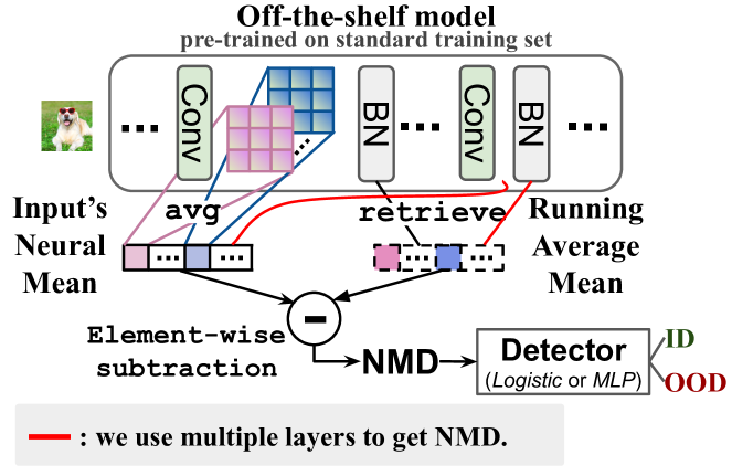
An overview of our approach is illustrated in Fig. 2. Our key idea is that, instead of constructing additional specialized witness function, one can instantiate the witness function using the off-the-shelf model pre-trained on the training data ${𝒟}_{\text{tr}}$. This witness function leads to the proposed metric, Neural Mean Discrepancy (NMD), which evaluates the statistics of neural activations from the off-the-shelf model.

3.1 Neural Mean Discrepancy

The supremum in Eq. 2 is taken over the witness function $\phi (\cdot )$, which implies that the neural network ${\phi }_{\omega }(\cdot )$ is optimized to maximize the discrepancy in expectation over $\mathbb{Q}$ and $\mathbb{P}$ [53, 11, 57]. This optimization leads to high computational cost. Instead, we propose to relax the requirement of supremum in the context of OOD detection by making an intuitive assumption: as long as a function is capable of differentiating the statistics (i.e., mean) of examples from in- and out-of- distributions in the projected (i.e., feature) space, this function can be a qualified witness function. Interestingly, we find the off-the-shelf model $f(\cdot )$ pre-trained on the in-distribution training set fits this criteria.

Taking a certain channel $c$ in the $l$-th layer of the off-the-shelf model as function $f_c^l:{ℝ}^{|ℐ|\times 3\times d^{\prime }\times d^{\prime }}\to {ℝ}^{|ℐ|\times 1\times d\times d}$, where $d^{\prime }$ and $d$ are the spatial sizes of input images and activation maps, respectively. We define a model-agnostic metric named Neural Mean Discrepancy (NMD) using $f_c^l$ as the witness function,

${\text{NMD}}_c^l(ℐ)=$ ${\displaystyle \frac{1}{|ℐ|\cdot d^2}}{\displaystyle \sum _{i=1}^{|ℐ|}}{\displaystyle \sum _{m=1}^d}{\displaystyle \sum _{n=1}^d}{f}_c^l{({𝐱}_i)}_{m,n}$ (3)

$-$ ${\displaystyle \frac{1}{|{𝒟}_{\text{tr}}|\cdot d^2}}{\displaystyle \sum _{j=1}^{|{𝒟}_{\text{tr}}|}}{\displaystyle \sum _{m=1}^d}{\displaystyle \sum _{n=1}^d}{f}_c^l{({𝐬}_j)}_{m,n}$ (4)

$=$ $𝝁[f_c^l(ℐ)]-𝝁[f_c^l({𝒟}_{\text{tr}})],$ (5)

where the first sum (${\sum }_{i=1}^{|ℐ|}$ or ${\sum }_{i=1}^{|{𝒟}_{\text{tr}}|}$) is taken over examples and the last two sums (${\sum }_{m=1}^d{\sum }_{n=1}^d$) are taken over all spatial positions $(m,n)$ in this channel.

We sum over spatial positions of the activation map because each kernel of a neural net can be viewed as a realization of the witness function in the IPM theory. Thus taking average over spatial positions within a channel (i.e., output of a kernel) is a faithful implementation of IPM with an NN.

Each spatial position responds to a corresponding patch from the input image, known as the receptive field [60, 59, 5]. As a result, averaging across spatial positions can be thought of as averaging over image patches after projecting them with $f_c^l$. This implicitly augments the input batch and enables our method to survive from an extremely small batch size $|ℐ|$ (even for a single input image $|ℐ|=1$) when compared to previous IPMs-based methods.

Multi-layer NMD for multi-scale OOD detection.

To further improve the performance, we consider measuring and combining NMDs from all channels across layers in the off-the-shelf model. By doing that, we can get an NMD vector for a given input batch $ℐ$,

which is a $C$-dimensional vector where $C$ is the total number of channels in the off-the-shelf model. The multi-layer NMD has three major advantages:

1. Each neural mean discrepancy ${\text{NMD}}_c^l$ associates with a unique witness function $f_c^l$. Our method utilises the combination of several witness functions which deliver richer capacity than previous approaches based on a single IPM, as validated by our extensive experiments.

2. ${\text{NMD}}_c^l$ for different layers may have different patch sizes because their receptive fields increase linearly with their layer depths. Combining NMDs from all layers enable multi-scale OOD detection which captures both low-level and high-level semantics (See Sec. 5.7).

3. By using multiple channels, NMD does not introduce extra computation overhead since they can be obtained via a single forward pass of the model.

“Free lunch” from Batch Normalization.

The way that NMD computes the activation statistics coincides with what Batch Normalization (BN) does. Rather than computing $𝝁[f_c^l({𝒟}_{\text{tr}})]$ by traversing the entire training data in Eq. 4, one can directly use the running average from BN.

BN is an indispensable component in modern DNNs due to its ability of stabilizing training and improving model generalizability [43]. BN computes an output which normalizes input using per-channel statistics. Concretely, in a given channel, BN subtracts the activation mean $\mu$ from the inputs and then divides them by standard deviation $\sigma$. During training, $\mu$ and ${\sigma }^2$ are the empirical per-channel mean ${\mu }_{\mathrm{batch}}$ and variance ${\sigma }_{\mathrm{batch}}^2$ of the current mini-batch. During testing $\mu$ and ${\sigma }^2$ are not computed from mini-batches. Instead, the expected statistics $\overline{\mu }$, ${\overline{\sigma }}^2$ are estimated from the training set and used for normalization. Ioffe et al. [43] proposes that running average can be used to efficiently estimate expected statistics,

where a typical value of $\lambda$ is $0.99$ (which is a standard way of implementation in most deep learning libraries [68, 2]).

Back to our method, we use the running average mean $\overline{\mu }$ stored in BN directly to approximate $𝝁[f_c^l({𝒟}_{\text{tr}})]$ instead of manually computing it with Eq. 4,

$$𝝁[f_c^l({𝒟}_{\text{tr}})]\approx {\overline{\mu }}_c^{\mathrm{\ell }}.$$ (8)

We adapt this approximation in our experiments and validate that it works efficiently for OOD detection. Besides, we also validate the effectiveness of Eq. 4 for models not containing BN (e.g., VGG [80] and Transformer [19]).

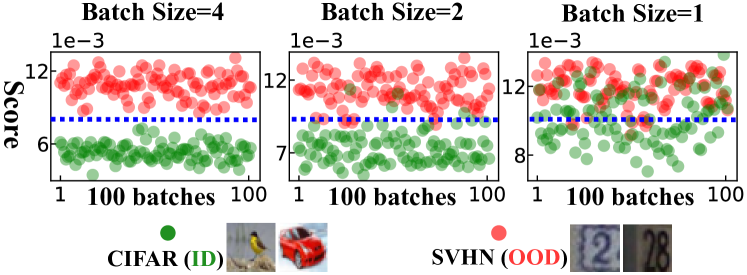
3.2 A proof of concept

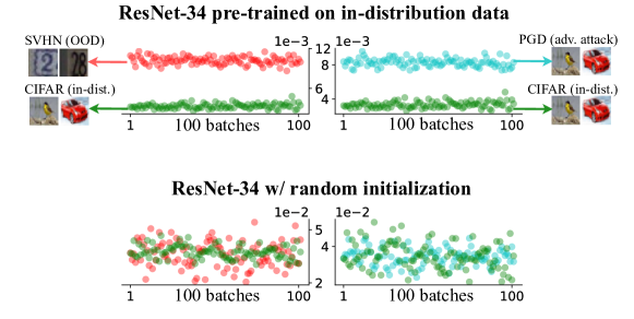
To verify our intuition using an example, we instantiate the in-distribution data using CIFAR-10 [47] and the out-of-distribution data using SVHN [67]. A ResNet-34 [35] is trained on CIFAR-10 with standard training receipt as the off-the-shelf model $f(\cdot )$. Given a mini-batch $ℐ$, its NMD vector is computed via Eqs. 5, 6 and 8. We propose an intuitive baseline method called Ours-Avg, which takes the average over elements’ magnitude in the NMD vector as confidence score for OOD detection. We randomly sample 100 mini-batches from CIFAR-10 (green dots) and SVHN (red dots) testing sets and visualize each batch’s score in Fig. 3. The observation in Fig. 3 validates our expectation: OOD data has larger NMD than in-distribution data on average.

Without any training, model fine-tuning, or hyper-parameter tuning, Ours-Avg achieves an impressive performance, 99.9% AUROC, with batch size $|ℐ|=4$. In contrast, other IPM-based methods typically require the batch size to be much larger [30, 70, 27].

3.3 A sensitivity-aware NMD detector

To further improve discriminatory power of the OOD detection, we propose to learn a parametric detector that takes NMD vectors as input instead of simply averaging them. By doing this, the detection performance is boosted even the batch size $|ℐ|$ drops to 1 (i.e., single input example).

Previous literature [32, 18, 9] observed that channels in deep neural networks are correlated and of different importance. To leverage this observation, we propose to train a detector $g(\cdot )$ that takes the NMD vector $\text{NMD}(𝐱)$ as input and predicts whether the current example is OOD or not. During training, these detectors are optimized on pairs of NMD representations and distribution indicators, e.g., $(\text{NMD}({𝐱}_{\mathrm{ID}}),0)$ for in-distribution examples and $(\text{NMD}({𝐱}_{\mathrm{OOD}}),1)$ for out-of-distribution ones.

These OOD detectors are simple, lightweighted, and efficient at both training and inference. We will demonstrate, in the experimental section, that the detector can learn with few-shot examples and has high generalizability to unseen OOD types. Even without access to OOD examples, the detector can still achieves superior performance by randomly permuting the pixels of in-distribution examples [73].

While the detector $g(\cdot )$ can be implemented using any classification method, we compare in our experiments two kinds of lightweight OOD detectors: a logistic regression $g_{\text{LR}}$ (LR) and a multilayer perceptron $g_{\text{MLP}}$ (MLP). The whole pipeline of our method can be found in Algorithm 1.

Algorithm 1 Pipeline of our NMD-based OOD detection

Input: (1) an input example $𝐱$,  (2) an off-the-shelf pre-trained classifier $f(\cdot )$, and  (3) an OOD detector ($g_{\text{LR}}$ or $g_{\text{MLP}}$).

Stage 1: Generate feature mean discrepancy vector

Do a forward pass with the off-the-shelf model $f\left(𝐱\right)$

for each channel in $f$ do

Compute ${\text{NMD}}_c^l\left(𝐱\right)$ via Eqs. 5, 6 and 8

end for

$\text{NMD}\left(𝐱\right)$ $\leftarrow$ Concatenate all channels’ ${\text{NMD}}_c^l\left(𝐱\right)$

Stage 2: Detect with the generated NMD vector $\text{NMD}\left(𝐱\right)$

if Training then

Train the OOD detector $g(\cdot )$ with pairs:   $\{(\text{NMD}\left({𝐱}_{\mathrm{ID}}\right),0),\mathrm{\dots },(\text{NMD}\left({𝐱}_{\mathrm{OOD}}\right),1)\}$

else if Testing then

Use the OOD detector $g\left(\text{NMD}\left(𝐱\right)\right)$ to get  the detecting result

end if

4 Experimental setup

Off-the-shelf models. NMD is model-agnostic and we evaluate it on multiple architectures, including 4-layer ConvNet [71, 44], ResNet-34 [35], self-supervised ResNet-34 [34], WideResNet [91], DenseNet-100 [40], VGG [80], and Vision Transformer [19]. All models are well-trained using their original training receipts and frozen (i.e., no fine-tuning) throughout the experiments.

Benchmark datasets. We perform comparative studies on various datasets: CIFAR-10, CIFAR-100, SVHN, cropped ImageNet, cropped LSUN, iSUN, and Texture, following OOD literature [55, 51, 73, 58, 78]. Different combinations of in- and out-of- distribution datasets result in different levels of difficulty. An OOD detection problem is typically categorized into near-OOD and far-OOD [84, 25, 72]. Near-OOD means that the two data distributions are close to each other. An example is using CIFAR-10 as in distribution and CIFAR-100 as OOD. This is because both datasets come from the same tinyimagenet dataset [69] and their labels are all daily objects with similar semantics. In contrast, an example for far-OOD could be CIFAR-10 as in distribution and SVHN as OOD because SVHN contains only house number images while CIFAR-10 contains natural images with rich information. Near-OOD is generally a harder task than far-OOD [78, 92, 73]. In order to demonstrate the effectiveness of our approach, we evaluate the NMD method in both near-OOD and far-OOD tasks.

Protocols. We consider 4 kinds of data access circumstances to simulate real-world OOD detection scenarios.

1. Full access: Conventional OOD detection approaches assume the access to both ID and OOD data for OOD detector training and hyper-parameter tuning.

2. Few-shot: Due to privacy concerns, the data owner may only release a few ID and OOD showcase examples for OOD detector training. In our experiments, we propose an extreme scenario where one only has access to 25 ID and 25 OOD examples for training.

3. Zero-shot: Recent studies [39, 58, 78, 90] also learn OOD detectors with only ID examples and without any dependence on OOD examples.

4. Transfer: To evaluate the transferability of different methods, we additionally propose to train the detectors on one kind of OOD dataset and evaluate their performance on separate unseen OOD datasets.

Evaluation metrics. Consistent with the literature [55, 51, 73, 58, 78], we use three evaluation metrics: (1) true negative rate at 95% true positive rate (TNR95), (2) area under the receiver operating characteristic curve (AUROC), and (3) detection accuracy (ACC) which measures the maximum detection accuracy over all possible thresholds.

Baseline methods. We compare our approach with several existing methods lying in different categories.

1. Statistical methods: These are most related to our work. As summarized in Sheng et al. [44], for a test example $𝐱$, such approaches compute the OOD score using the negative of the sum of kernel evaluation at each of the inlier example ${𝒮}_{{𝐱}^{\prime }}$ such that $\text{score}(𝐱)=-{\sum }_{i=1}^{|𝒮|}\kappa (𝐱,{𝐱}_i^{\prime })$. Different choices of the kernel $\kappa$ result in different methods including Deep kernel (DK [57, 27]), convolution neural tangent kernel (CNTK [6]), and shift-invariant convolutional neural tangent kernel (SCNTK [44]).

2. Other baselines: We also compare our method with other state-of-the-art approaches such as ODIN [55], Mahalanobis distance [51], OE with classifier fine-tuning [38], and Energy with classifier fine-tuning [58]. They require model fine-tuning, hyper-parameter tuning, multi-round forward inference, while NMD does not depend on any of the above.

5 Results

We show our results in this section, which empirically demonstrate the simplicity, efficacy, efficiency, and generalizability of NMD-based OOD detection. All results are obtained for single example detection, i.e., batch size $|ℐ=1|$.

5.1 Comparison with statistical baselines

We first compare our method with the most related line of approaches based on statistical tests, i.e., DK [57, 27], CNTK [6], and SCNTK [44]. These methods require a traversing in a subset of the in-distribution data ${𝒮}_{{𝐱}^{\prime }}$ for every test example, which could be expensive. NMD does not depend on ${𝒮}_{{𝐱}^{\prime }}$ which leads to higher efficiency. Following settings of Sheng et al. [44], all compared methods adapt a four-layer convolutional neural network as the feature extractor. Tab. 1 shows that our method (using logistic regression detection, denoted as ‘Ours-LR’) achieves significantly better OOD detection performance (99.8+% AUROC). The result empirically justifies the value of using multiple witness functions at different scales and semantic levels from the same pre-trained model.

Model	ID	OOD	Method	AUROC
ConvNet (4 layers)	CIFAR-10	SVHN	DK	82.4
			CNTK	71.3
			SCNTK	84.9
			Ours-LR	99.9
ConvNet (4 layers)	SVHN	CIFAR-10	DK	21.4
			CNTK	51.9
			SCNTK	80.3
			Ours-LR	99.8

Table 1: AUROC comparison of statistical OOD detection methods. we compare our method with deep kernel on extracted feature maps (DK) [57, 27], convolutional neural tangent kernel (CNTK) [6], shift-invariant convolutional neural tangent kernel (SCNTK) [44]. Consistent to the setting of [44], we use a four-layer convolution neural network as the classifier for feature extraction. More details can be found in the appendix.

5.2 Comparison with other baselines

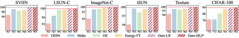
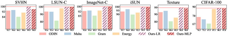
We evaluate our method on a set of out-of-distribution datasets with ResNet trained on the in-distribution dataset CIFAR-10. In this experiment, we assume both the ID and OOD datasets are available for training. The pre-trained ResNet-34 is frozen in our NMD method, while other methods may further fine-tune it to maximize the test power. In addition, our NMD is hyper-parameter free while other approaches may have sensitive hyper-parameters to tune (e.g., temperatures in [55], perturbation in [51], and margin in [58]). As shown in Fig. 4, despite its simplicity, our method consistently outperforms other methods across datasets, especially on near-OOD dataset, CIFAR-100. More experimental results can be found in the appendix.

Figure 4: AUROC comparison with OOD methods requiring both in- and out-of- distribution data for detector training, classifier fine-tuning or hyper-parameter search. We compare our method with ODIN [55], Maha [51], OE with fine-tuning [38], and Energy with fine-tuning [58] on ResNet-34, using CIFAR-10 as in-distribution. The Energy method is finetuned using each of the OOD training sets.

Figure 5: AUROC comparison of detection methods when only in-distribution dataset is accessible. We compared our method with Energy without classifier fine-tuning [58], Gram [78], G-ODIN [39], and 1D [90] on ResNet-34, using CIFAR-10 as in-distribution dataset.

Figure 6: AUROC comparison of detection methods when only 25 in- and 25 out-of- distribution examples are accessible. We compared our method with ODIN, Maha, Gram, and Energy with classifier fine-tuning [58] on ResNet-34, using CIFAR-10 as in-distribution dataset.

5.3 Learning with only in-distribution examples

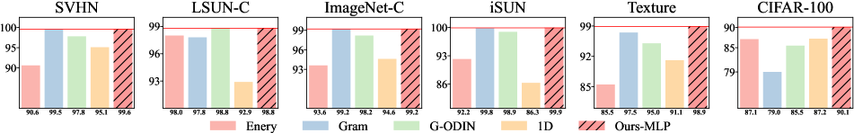
We further compare our method with approaches that do not depend on any given OOD dataset for training. Among them, G-ODIN [39] and 1D [90] need to fine-tune the model on in-distribution dataset. Since no OOD example is accessible, we craft artificial OOD examples by randomly permuting pixels of in-distribution examples and use the crafted OOD examples to train our detector. The detector trained on artificial OOD examples is evaluated on realistic OOD datasets. Fig. 5 shows that our method performs better than state-of-the-art without access to realistic OOD data. The result also suggests that, even though the artificial OOD examples are unrealistic, they are helpful in guiding the decision boundary of an OOD detector.

5.4 Few-shot OOD training

We evaluate our method under the scenario that a very limited number of in-distribution and out-of-distribution examples are available for training.

Fig. 6 compares different methods when only 25 ID examples and 25 OOD examples are present during training. The baseline ‘Gram’ uses 50 ID examples as an exception because it does not depend on OOD examples. Since 50 examples are too few to conduct fine-tuning for ‘Energy’, we report its performance without fine-tuning as a reference.

Our method outperforms all other methods under this few-shot setting. Previous works often require sufficient data to tune hyper-parameters or models. In contrast, NMD is hyper-parameter-free and thus can learn well with few examples. However, we observe a slight over-fitting of the MLP detector which suggests one should consider low-capacity models such as LR in the few-shot cases.

In-dist.	Train OOD	Test OOD	ResNet-34	ResNet-34 (self)	VGG-19	ViT	DenseNet
			TNR at TPR 95% $\uparrow$ / AUROC $\uparrow$ / ACC $\uparrow$
CIFAR-10	CIFAR-100	LSUN-C	95.8 / 99.2 / 95.6	99.1 / 99.8 / 98.1	96.4 / 99.3 / 95.7	94.0 / 98.7 / 94.6	90.6 / 98.3 / 93.6
		SVHN	96.4 / 99.2 / 95.9	99.9 / 99.9 / 99.9	99.9 / 99.9 / 99.1	99.8 / 99.9 / 99.2	95.8 / 99.2 / 95.4
		Texture	91.7 / 98.5 / 93.4	97.8 / 99.5 / 96.7	96.1 / 99.1 / 95.6	91.4 / 98.3 / 93.5	93.0 / 98.6 / 94.0
		ImageNet-C	93.7 / 98.7 / 94.4	99.9 / 99.9 / 99.1	94.0 / 98.9 / 94.5	89.0 / 98.1 / 93.0	94.3 / 98.8 / 94.7

Table 2: We evaluate generalizability of our method across models, including ResNet-34 trained with standard softmax cross-entropy loss [35], ResNet-34 trained with self-supervised loss from MoCo [34], VGG-19 (without BN) [80], and Visual Transformer [19]. To further validate the generalizability across datasets, we use CIFAR-100 as OOD dataset to train our detector and test the trained detector on unseen OOD datasets including LSUN-C, SVHN, Texture, and ImageNet-C.

5.5 Generalizability across models and datasets

We are interested in the transferability of the detector across datasets. For each model, we use CIFAR-100 as OOD dataset for training the detector and evaluate the trained detector on unseen OOD datasets such as LSUN-C, SVHN, Texture, and ImageNet-C.

As we elaborated in Sec. 3.1, one can either use running average in BN to approximate $𝝁[f_c^l({𝒟}_{\text{tr}})]$ (Eq. 8) or manually compute it via Eq. 4 if the model has no BN layers. So we also evaluates the generalizability of our method across different models.

1. VGG models. VGG-19 consists of 16 convolution and ReLU layers, followed by three fully-connected (FC) layers. It has no BN layers. We only use channels from convolutional layers to compute NMD. Since no BN layer is present in this model, we traverse the in-distribution training set (i.e., CIFAR-10) for one epoch.

2. Self-supervised models. We use MoCo [34] as the self-supervised learning method. After pre-training a ResNet-34 model with MoCo on CIFAR-10, we freeze it and use it to compute NMD.

3. Vision Transformers. Different from CNNs, a Vision Transformer (ViT) [19] is composed of a stack of standard multi-head self-attention and position-wise fully-connected layers. ViT splits an image into $p$ non-overlapped patches and provides the sequence of embeddings of these patches as an input to a Transformer. ViT adopts layer normalization (LN) [8] to normalize each input example’s activation ${𝐙}^l\in {ℝ}^{p\times d}$. Imitating convolution neural networks, we compute ViT’s feature mean for an input example $𝐱$ with ${𝝁}^l\left(𝐱\right)=\frac{1}{p}{\sum }_{i=1}^p{\text{Z}}_i^l\in {\mathrm{\Re }}^d$, and use it to compute NMD metric.

Tab. 2 indicates that NMD generalizes well for various models and datasets. Interestingly, we find that self-supervised ResNet-34 has the best averaged detection performance across 4 unseen OOD datasets, suggesting the high transferability of its learnt representations [34, 16, 23].

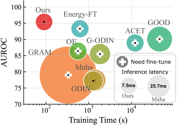
5.6 Training and inference efficiency

In this section, we compare the training and inference costs of the proposed Ours-MLP with baselines in Fig. 1. We measure the training and inference time on a machine with one NVIDIA GPU 1080 Ti and a Intel(R) Xeon(R) CPU E5-2650 v4 @ 2.20GHz.

Training cost. Since the detectors (i.e., LR and MLP) we used are lightweight, the training process can be done quickly (within 60 epochs with CIFAR-10 (ID) and CIFAR-100 (OOD) training datasets in Fig. 1). In addition, different from existing methods, NMD does not have sensitive hyperparameters and thus does not have to repeat training process for multiple times to search the hyperparameters.

Inference cost. As illustrated in Algorithm 1, we only have to run a single forward pass with the pre-trained model to generate the NMD vector. The generated NMD vector will be then processed by a lightweight detector (e.g., Logistic regress or three-layer MLP as detailed in Sec. 3.3). In contrast, other approaches, in addition to a standard forward pass (Baseline [37] and ACET [36]), also require either: (1) extra forward and backward passes [39, 51, 55]; (2) computing complicated properties (e.g., co-occurrences) [78, 90].

5.7 Ablation study

Layer importance for OOD detection.

Figure 7: We study the layer-granularity importance of ResNet-34 for far-OOD (e.g., SVHN, left) and near-OOD (e.g., CIFAR-100, right) using CIFAR-10 as in-distribution dataset. Top figures: Importance of each layer in ResNet-34, where a layer’s importance is measured by the averaged magnitude of channels’ coefficients in the LR detector. Bottom figures: We use the first $k$ layers (x-axis) to do detection and evaluate the AUROC for different $k$.

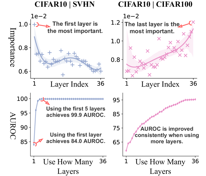
We visualize the importance of NMD from different layers of ResNet-34 in Fig. 7. We find that our method utilises both low-level visual attributes (from shallow layers) as well as high-level semantic information (from deep layers) and dynamically adjusts the importance depending on tasks. In the top two plots of Fig. 7, we specify the OOD detector as a logistic regression (LR). We standardize NMD vector to ensure that each of its dimensions has a similar magnitude before sending it to the LR model.

The absolute values of each learned coefficient in LR can be treated as the importance of its corresponding channel. We compute a layer’s importance by averaging all its channels’ importance values. We test two OOD detection tasks: (1) In a far-OOD task CIFAR-10 against SVHN, NMD values from shallow layers, which extract low-level features [88, 7], are already able to differentiate CIFAR-10 against SVHN. (2) In a near-OOD task, CIFAR-10 against CIFAR-100, we have to rely more on NMD values from deeper layers to capture the semantic differences.

In the bottom two plots of Fig. 7, we visualize the detection performance when the first $k$ layers’ NMDs are used. For SVHN, it is sufficient to achieve the best AUROC with only the first 5 layers. While, for CIFAR-100, using more layers consistently leads to better performance. This observation aligns well with the previous paragraph, and motivates a potential future work on dynamically selecting layers given an input example (i.e., ‘early exits’) for better performance and efficiency like [56].

Does Neural Variance Discrepancy help? Besides the first order statistics (i.e., mean), one can define Neural Variance Discrepancy (NVD) by computing the activation’s second-order statistics in a similar manner. In practise, we find that using NVD (AUROC=95.3, CIFAR-10 against CIFAR-100 on ResNet-34) is able to achieve a similar OOD detection performance as NMD (AUROC=95.4). Combining both NMD and NVD obtains a slightly better result (AUROC=95.6). Please refer to Appendix E for more details.

6 Related work

OOD detection with model modification and fine-tuning. Multiple OOD approaches augment standard DNN architectures by model ensemble [26, 48, 83, 14], training an additional branch [17, 33], and learning a background model [73]. In addition, various novel training objectives have been proposed including training with OOD uniform label [50], an additional OOD class [15, 61], OOD examples crafted by a generative model [62], energy score regualarization [58], and soft-binning error [45].

OOD detection without fine-tuning. Maximum softmax probability [37] and it variants like ODIN [55], GODIN [39], POOD [24] and Energy [58] have been used for OOD detction. Beside the final outputs, intermediate activation is also used like Gram [78], Mahalanobis [51, 72].

Statistical OOD detection. Previous studies have shown some preliminary results of using Frechet distance [20] and Maximum Mean Discrepancy (MMD) [29] for adversarial [30, 13, 27, 74] and distribution shift detection [70, 31]. Erdil et al. [22] applies adversarial perturbation and kernel density estimation (KDE) for a subset of in-distribution examples and each input to do OOD detection. Density of states estimator is also used for OOD detection with generative models [63]. Jia et al. [44] proposes a compositional kernel, as a variates of adaptive deep neural kernel [57, 27, 6], for efficient OOD detection. However, mere shallow models are considered. In this work, by creatively leveraging neural means from a pre-trained model, we significantly reduce the algorithmic complexity and computational cost of statistical OOD detection.

Updating Batch Normalization statistics for improved accuracy. Previous studies find that one can improve model performance by updating the statistics and affine parameters of the Batch Norm layers when either data or model change during training [82, 75] or testing [65, 89]. Such BN recalibration techniques show promising effectiveness of improving the model performance [85, 42], domain adaptation and generalization ability [54, 77], few-shot learning [21], and the model’s robustness against input noise [79, 66, 10].

7 Conclusion and discussion

We proposed Neural Mean Discrepancy (NMD) which compares the neural means between test examples and training data for OOD detection. Both the IPMs-based theoretical analysis and empirical results validate the efficacy of NMD. With the extreme algorithmic simplicity, NMD is evaluated across datasets, models, and data access circumstances, achieving state-of-the-art accuracy and efficiency.

Limitations.

Although NMD can achieve competitive results without access to real OOD data (see Sec. 5.3), artificially crafted OOD data via pixel shuffling is still required to learn channel sensitivities. It is likely to estimate sensitivities directly via weight distributions of the off-the-shelf model [87, 41] or gradient information [81, 4]. In addition, early existing works [3, 56] could be applied to further improve the performance of an NMD-based OOD detector.

Appendix A Extra Results Using Different In-Distribution Datasets

We further evaluate our method on various in-distribution datasets including SVHN and CIFAR-100 in Tab. 3 using the same setting as Fig. 4. According to Fig. 4, our method achieves state-of-the-art results with various in-distribution datasets.

In-dist. (model)	OOD	Baseline [37]	ODIN [55]	Maha. [51]	Ours-LR
CIFAR-100 (ResNet-34)	SVHN	79.5	70.7	92.4	94.2
	LSUN-C	75.8	85.6	98.2	99.9
	ImageNet-C	77.2	87.8	98.0	99.9
SVHN (ResNet-34)	CIFAR-10	92.9	92.1	99.3	99.8
	LSUN-R	91.6	89.4	99.9	99.9
	ImageNet-R	93.5	92.0	99.9	99.9
CIFAR-100 (DenseNet-100)	SVHN	82.7	85.2	90.3	93.3
	LSUN-C	70.8	85.5	98.0	99.9
	ImageNet-C	71.6	84.8	94.1	99.6

Table 3: AUROC comparison of detection methods on various in-distribution datasets.

Figure 8: We redo the proof-of-concept experiment in Fig. 3 with an un-trained ResNet-34. The batch size is 8.

Appendix B Lightweight OOD Detector

• Logistic regression (LR) is a kind of classic machine learning model for binary classification. Given an input vector, The LR model performs a dot product on the input with the learned coefficient vector and outputs the prediction score after applying the sigmoid function. A LR model can be trained efficiently by several solvers like LBFGS. [52] We use the default hyper-parameters in sklearn [1] for training of LR detector.

• The multilayer perceptron (MLP) we use consists of three full-connected layers following by non-linear activation function ReLU. We adapt dropout after the second full-connected layer and train the MLP with SGD optimizer. As a non-linear model, MLP is able to learn more complex correlation among elements in the input than LR. In practise, we find that MLP has slightly better detection performance than LR, while, with higher over-fitting possibility when the number of training examples is limited. We training the MLP using SGD with 0.001 learning rate and 0.9 momentum.

The adapted OOD detector is lightweight. For instance, Our LR model has 8k parameters and 16k FLOPs, significantly smaller than the pre-trained model (e.g., ResNet-34 with $\sim$2$\times {10}^4$k parameters and $\sim$2$\times {10}^6$k FLOPs).

Appendix C Architecture of ConvNet

Consistent to the setting of [44], we use a simple ConvNet in Secs. 5.1 and 1. ConvNet’s architecture is summarized in Tab. 4.

Layer	Configuration
Conv1	(3, 300, kernel size=4, stride=1)
Conv2	(300, 300, kernel size=4, stride=2)
Conv3	(300, 300, kernel size=4, stride=2)
Conv4	(300, 300, kernel size=3, stride=2)
AvgPool	(kernel size=2)
FC	(300, 10)

Table 4: Architecture of ConvNet following [44]. After each convolutional layer, batch normalization and ReLU layers are applied.

Appendix D Pre-trained or Un-trained Models?

In Fig. 3, we show that the average of elements’ magnitude in NMD vector from a pre-trained ResNet-34 can be used as OOD score to reliably distinguish OOD batches. Such a proof-of-concept example validates that the off-shelf-shelf pre-trained model can be used as a qualified witness function. Based on this interesting and supervising finding, we believe the off-the-shelf model itself should contain sufficient information about the training data distribution because it was trained to capture training data’s features.

To further validate our hypothesis, we replace the pre-trained ResNet-34 with an un-trained ResNet-34 and re-run the experiment. As shown in Fig. 8, an un-trained ResNet-34 cannot act as a qualified witness function to detect OOD batches even the batch size is 8.

Appendix E Neural Variance Discrepancy

As mentioned in Sec. 5.7, one can define Neural Variance Discrepancy (NVD) by computing the activation’s second-order statistics in a similar manner as NMD,

${\text{NVD}}_c^l(ℐ)=\sqrt{{𝝈}^{\mathrm{𝟐}}[f_c^l(ℐ)]}-\sqrt{{𝝈}^{\mathrm{𝟐}}[f_c^l({𝒟}_{\text{tr}})]},$ (9)

where the second term can be approximated by BN’s running average variance. Interestingly, NVD-based detection (i.e., NVD-MLP) achieves a comparable detection performance as NMD.

We further combine NVD and NMD via concatenating them together. Since elements in NVD and NMD may have different magnitude, we adopt the standardizer from sklearn to remove the mean and scale to unit variance for each dimension of NVM and NMD vectors before concatenating. Combining NMD and NVD obtains a slightly better detection result although extra computation overhead is introduced.

Appendix F Crafting OOD Data by Pixel Permuting

As discussed in Sec. 5.3, if no OOD example is accessible, we craft artificial OOD examples by randomly permuting pixels of in-distribution examples and use the crafted OOD examples to guide our detector for finding the decision boundary. The premise of using crafted OOD example is that the method has high generalizability across datasets (i.e., for unseen OOD data) as validated in Sec. 5.5. Specifically, we do pixel permuting in the block granularity instead of in the pixel granularity [73] to avoid tuning the hyperparameter “mutation rate”. Taking CIFAR-10 example as an example, we split an image into 16 non-overlapping ($8\times 8$) blocks and randomly permute their positions. Results of detection performance without OOD examples are shown in Figs. 5 and 6.

Appendix G Training and Inference Efficiency

In Sec. 5.6, we compare the training and inference costs of the proposed Ours-MLP with baselines as shown in Fig. 1. Training and inference time are measured on a machine with one NVIDIA GPU 1080 Ti and a Intel(R) Xeon(R) CPU E5-2650 v4 @ 2.20GHz. Some approaches conduct model fine-tuning using MIT 80 Million Tiny Images Dataset which is not available any more. For those methods, we use the target OOD dataset (i.e., CIFAR-100 training set) to do fine-tuning but with the same number of iterations as using MIT 80 Million Tiny Images Dataset. For methods which require repeating experiments for several times to search hyper-parameters, we count all such time into training time. To measure the inference latency, we repeat single example detection for 10,000 times and compute the average inference time for a single example.

A recent study, MOOD [56], achieves state-of-the-art inference efficiency leveraging early exiting [3]. We do not include MOOD in Tab. 5 because it depends a special architecture with dynamic exits. In addition, our method is orthogonal to MOOD and could be combined for a future work as discussed in Secs. 5.7 and 7.

Method	Fine-tuning	Training	Inference
Gram	True	330s	0.37s
Maha	False	1397s	25.7ms
ODIN	False	1270s	16.0ms
G-ODIN	True	1830s	22.1ms
OE	True	560s	6.72ms
GOOD	True	756m	47.4ms
ACET	True	201m	6.89ms
Energy-FT	True	620s	7.24ms
Plain ResNet-34	-	-	6.72ms
Ours-MLP	False	94s	7.54ms

Table 5: Training and inference time comparison with CIFAR-10against CIFAR-100 (OOD) detection on ResNet-34. (Also see Fig. 1)

In-dist (model)	OOD	Energy (w/o FT)	Gram (w/o FT)	G-ODIN (w/ FT)	1D (w/ FT)	Ours-MLP (w/o FT)
		TNR at TPR 95% / AUROC / Detection acc.
CIFAR-10 (ResNet-34)	iSUN	60.4 / 92.2 / 87.0	99.3 / 99.8 / 98.1	95.3 / 98.9 / 95.6	76.9 / 86.3 / 92.9	99.7 / 99.9 / 98.6
	SVHN	58.4 / 90.6 / 85.5	97.6 / 99.5 / 96.7	89.5 / 97.8 / 92.9	86.2 / 95.1 / 88.9	97.7 / 99.6 / 96.6
	Texture	41.1 / 85.5 / 80.8	88.0 / 97.5 / 91.9	81.4 / 95.0 / 88.9	72.4 / 91.1 / 84.9	94.0 / 98.9 / 94.6
	LSUN-C	89.2 / 98.0 / 93.8	89.8 / 97.8 / 92.6	93.9 / 98.8 / 94.0	77.1 / 92.9 / 86.5	93.9 / 98.8 / 94.5
	ImageNet-C	67.4 / 93.6 / 88.7	96.7 / 99.2 / 96.1	90.8 / 98.2 / 94.3	81.9 / 94.6 / 88.5	96.1 / 99.2 / 95.6
	CIFAR-100	43.1 / 87.1 / 80.7	32.9 / 79.0 / 71.7	36.3 / 85.5 / 79.3	57.4 / 87.2 / 80.8	63.8 / 90.1 / 83.4

Table 6: Comparison of detection methods when only in-distribution dataset is accessible. (Also see Fig. 5)

References

- [1] sklearn.linear_model.logisticregressioncv.
- [2] Martín Abadi, Paul Barham, Jianmin Chen, Zhifeng Chen, Andy Davis, Jeffrey Dean, Matthieu Devin, Sanjay Ghemawat, Geoffrey Irving, Michael Isard, et al. Tensorflow: A system for large-scale machine learning. In 12th USENIX symposium on operating systems design and implementation (OSDI 16), pages 265–283, 2016.
- [3] Vahdat Abdelzad, Krzysztof Czarnecki, Rick Salay, Taylor Denounden, Sachin Vernekar, and Buu Phan. Detecting out-of-distribution inputs in deep neural networks using an early-layer output. arXiv preprint arXiv:1910.10307, 2019.
- [4] Amina Adadi and Mohammed Berrada. Peeking inside the black-box: a survey on explainable artificial intelligence (xai). IEEE access, 6:52138–52160, 2018.
- [5] André Araujo, Wade Norris, and Jack Sim. Computing receptive fields of convolutional neural networks. Distill, 2019. https://distill.pub/2019/computing-receptive-fields.
- [6] Sanjeev Arora, Simon S. Du, Wei Hu, Zhiyuan Li, Ruslan Salakhutdinov, and Ruosong Wang. On exact computation with an infinitely wide neural net. In Thirty-third Conference on Neural Information Processing Systems, 2019.
- [7] Yuki M Asano, Christian Rupprecht, and Andrea Vedaldi. A critical analysis of self-supervision, or what we can learn from a single image. ICLR, 2020.
- [8] Jimmy Lei Ba, Jamie Ryan Kiros, and Geoffrey E Hinton. Layer normalization. arXiv preprint arXiv:1607.06450, 2016.
- [9] David Bau, Bolei Zhou, Aditya Khosla, Aude Oliva, and Antonio Torralba. Network dissection: Quantifying interpretability of deep visual representations. In Proceedings of the IEEE conference on computer vision and pattern recognition, pages 6541–6549, 2017.
- [10] Philipp Benz, Chaoning Zhang, and In So Kweon. Batch normalization increases adversarial vulnerability and decreases adversarial transferability: A non-robust feature perspective. In CVPR, 2021.
- [11] Mikołaj Bińkowski, Dougal J Sutherland, Michael Arbel, and Arthur Gretton. Demystifying mmd gans. ICLR, 2018.
- [12] Julian Bitterwolf, Alexander Meinke, and Matthias Hein. Certifiably adversarially robust detection of out-of-distribution data. NeurIPS, 2020.
- [13] Nicholas Carlini and David Wagner. Adversarial examples are not easily detected: Bypassing ten detection methods. In Proceedings of the 10th ACM Workshop on Artificial Intelligence and Security, 2017.
- [14] Changjian Chen, Jun Yuan, Yafeng Lu, Yang Liu, Hang Su, Songtao Yuan, and Shixia Liu. Oodanalyzer: Interactive analysis of out-of-distribution samples. IEEE transactions on visualization and computer graphics, 27(7):3335–3349, 2020.
- [15] Jiefeng Chen, Yixuan Li, Xi Wu, Yingyu Liang, and Somesh Jha. Informative outlier matters: Robustifying out-of-distribution detection using outlier mining. ICML workshop on Uncertainty and Robustness in Deep Learning, 2020.
- [16] Ting Chen, Simon Kornblith, Kevin Swersky, Mohammad Norouzi, and Geoffrey Hinton. Big Self-Supervised Models are Strong Semi-Supervised Learners. NeurIPS, Oct. 2020.
- [17] Terrance DeVries and Graham W Taylor. Learning confidence for out-of-distribution detection in neural networks. arXiv preprint arXiv:1802.04865, 2018.
- [18] Xin Dong, Shangyu Chen, and Sinno Jialin Pan. Learning to prune deep neural networks via layer-wise optimal brain surgeon. NeurIPS, 2017.
- [19] Alexey Dosovitskiy, Lucas Beyer, Alexander Kolesnikov, Dirk Weissenborn, Xiaohua Zhai, Thomas Unterthiner, Mostafa Dehghani, Matthias Minderer, Georg Heigold, Sylvain Gelly, Jakob Uszkoreit, and Neil Houlsby. An image is worth 16x16 words: Transformers for image recognition at scale. ICLR, 2021.
- [20] DC Dowson and BV Landau. The fréchet distance between multivariate normal distributions. Journal of multivariate analysis, 12(3):450–455, 1982.
- [21] Yingjun Du, Xiantong Zhen, Ling Shao, and Cees GM Snoek. Metanorm: Learning to normalize few-shot batches across domains. In International Conference on Learning Representations, 2020.
- [22] Ertunc Erdil, Krishna Chaitanya, Neerav Karani, and Ender Konukoglu. Task-agnostic out-of-distribution detection using kernel density estimation. arXiv preprint arXiv:2006.10712, 2021.
- [23] Linus Ericsson, Henry Gouk, and Timothy M Hospedales. How Well Do Self-Supervised Models Transfer? CVPR, 2021.
- [24] Tajwar et al. No true state-of-the-art? ood detection methods are inconsistent across datasets. ICML Workshop on URDL, 2021.
- [25] Stanislav Fort, Jie Ren, and Balaji Lakshminarayanan. Exploring the limits of out-of-distribution detection. NeurIPS, 2021.
- [26] Yarin Gal and Zoubin Ghahramani. Dropout as a bayesian approximation: Representing model uncertainty in deep learning. In international conference on machine learning, pages 1050–1059. PMLR, 2016.
- [27] Ruize Gao, Feng Liu, Jingfeng Zhang, Bo Han, Tongliang Liu, Gang Niu, and Masashi Sugiyama. Maximum mean discrepancy is aware of adversarial attacks. In ICML, 2021.
- [28] Ian Goodfellow, Yoshua Bengio, and Aaron Courville. Deep learning. MIT press, 2016.
- [29] Arthur Gretton, Karsten M Borgwardt, Malte J Rasch, Bernhard Schölkopf, and Alexander Smola. A kernel two-sample test. The Journal of Machine Learning Research, 13(1):723–773, 2012.
- [30] Kathrin Grosse, Praveen Manoharan, Nicolas Papernot, Michael Backes, and Patrick McDaniel. On the (statistical) detection of adversarial examples. arXiv:1702.06280, 2017.
- [31] Devin Guillory, Vaishaal Shankar, Sayna Ebrahimi, Trevor Darrell, and Ludwig Schmidt. Predicting with confidence on unseen distributions. In Proceedings of the IEEE/CVF International Conference on Computer Vision, pages 1134–1144, 2021.
- [32] Song Han, Jeff Pool, John Tran, and William J Dally. Learning both weights and connections for efficient neural networks. NeurIPS, 2015.
- [33] Marton Havasi, Rodolphe Jenatton, Stanislav Fort, Jeremiah Zhe Liu, Jasper Snoek, Balaji Lakshminarayanan, Andrew M Dai, and Dustin Tran. Training independent subnetworks for robust prediction. ICLR, 2021.
- [34] Kaiming He, Haoqi Fan, Yuxin Wu, Saining Xie, and Ross Girshick. Momentum contrast for unsupervised visual representation learning. In Proceedings of the IEEE/CVF Conference on Computer Vision and Pattern Recognition, pages 9729–9738, 2020.
- [35] Kaiming He, Xiangyu Zhang, Shaoqing Ren, and Jian Sun. Deep residual learning for image recognition. In Proceedings of the IEEE conference on computer vision and pattern recognition, pages 770–778, 2016.
- [36] Matthias Hein, Maksym Andriushchenko, and Julian Bitterwolf. Why relu networks yield high-confidence predictions far away from the training data and how to mitigate the problem, 2019.
- [37] Dan Hendrycks and Kevin Gimpel. A baseline for detecting misclassified and out-of-distribution examples in neural networks. arXiv preprint arXiv:1610.02136, 2016.
- [38] Dan Hendrycks, Mantas Mazeika, and Thomas Dietterich. Deep anomaly detection with outlier exposure. ICLR, 2019.
- [39] Yen-Chang Hsu, Yilin Shen, Hongxia Jin, and Zsolt Kira. Generalized odin: Detecting out-of-distribution image without learning from out-of-distribution data. In Proceedings of the IEEE/CVF Conference on Computer Vision and Pattern Recognition, pages 10951–10960, 2020.
- [40] Gao Huang, Zhuang Liu, Laurens Van Der Maaten, and Kilian Q Weinberger. Densely connected convolutional networks. In Proceedings of the IEEE conference on computer vision and pattern recognition, pages 4700–4708, 2017.
- [41] Zhongzhan Huang, Wenqi Shao, Xinjiang Wang, Liang Lin, and Ping Luo. Convolution-weight-distribution assumption: Rethinking the criteria of channel pruning. NeurIPS, 2021.
- [42] Itay Hubara, Yury Nahshan, Yair Hanani, Ron Banner, and Daniel Soudry. Accurate post training quantization with small calibration sets. In ICML, pages 4466–4475. PMLR, 2021.
- [43] Sergey Ioffe and Christian Szegedy. Batch normalization: Accelerating deep network training by reducing internal covariate shift. In ICML, pages 448–456. PMLR, 2015.
- [44] Sheng Jia, Ehsan Nezhadarya, Yuhuai Wu, and Jimmy Ba. Efficient statistical tests: A neural tangent kernel approach. In ICML, pages 4893–4903. PMLR, 2021.
- [45] Archit Karandikar, Nicholas Cain, Dustin Tran, Balaji Lakshminarayanan, Jonathon Shlens, Michael C Mozer, and Becca Roelofs. Soft calibration objectives for neural networks. NeurIPS, 2021.
- [46] Matthias Kirchler, Shahryar Khorasani, Marius Kloft, and Christoph Lippert. Two-sample testing using deep learning. In AISTATS, 2020.
- [47] Alex Krizhevsky, Geoffrey Hinton, et al. Learning multiple layers of features from tiny images. 2009.
- [48] Balaji Lakshminarayanan, Alexander Pritzel, and Charles Blundell. Simple and scalable predictive uncertainty estimation using deep ensembles. Advances in neural information processing systems, 30, 2017.
- [49] Yann LeCun, Yoshua Bengio, and Geoffrey Hinton. Deep learning. nature, 521(7553):436–444, 2015.
- [50] Kimin Lee, Honglak Lee, Kibok Lee, and Jinwoo Shin. Training confidence-calibrated classifiers for detecting out-of-distribution samples. ICLR, 2017.
- [51] Kimin Lee, Kibok Lee, Honglak Lee, and Jinwoo Shin. A simple unified framework for detecting out-of-distribution samples and adversarial attacks. NeurIPS, 2018.
- [52] Su-In Lee, Honglak Lee, Pieter Abbeel, and Andrew Y Ng. Efficient l~ 1 regularized logistic regression. In Aaai, volume 6, pages 401–408, 2006.
- [53] Chun-Liang Li, Wei-Cheng Chang, Yu Cheng, Yiming Yang, and Barnabás Póczos. Mmd gan: Towards deeper understanding of moment matching network. NeurIPS, 2017.
- [54] Yanghao Li, Naiyan Wang, Jianping Shi, Xiaodi Hou, and Jiaying Liu. Adaptive batch normalization for practical domain adaptation. Pattern Recognition, 80:109–117, 2018.
- [55] Shiyu Liang, Yixuan Li, and Rayadurgam Srikant. Enhancing the reliability of out-of-distribution image detection in neural networks. ICLR, 2018.
- [56] Ziqian Lin, Sreya Dutta Roy, and Yixuan Li. MOOD: Multi-Level Out-of-Distribution Detection. CVPR, 2021.
- [57] Feng Liu, Wenkai Xu, Jie Lu, Guangquan Zhang, Arthur Gretton, and Danica J Sutherland. Learning deep kernels for non-parametric two-sample tests. In ICML, pages 6316–6326. PMLR, 2020.
- [58] Weitang Liu, Xiaoyun Wang, John D Owens, and Yixuan Li. Energy-based out-of-distribution detection. NeurIPS, 2020.
- [59] Wenjie Luo, Yujia Li, Raquel Urtasun, and Richard Zemel. Understanding the effective receptive field in deep convolutional neural networks. In NeurIPS, 2016.
- [60] Masakazu Matsugu, Katsuhiko Mori, Yusuke Mitari, and Yuji Kaneda. Subject independent facial expression recognition with robust face detection using a convolutional neural network. Neural Networks, 2003.
- [61] Sina Mohseni, Mandar Pitale, JBS Yadawa, and Zhangyang Wang. Self-supervised learning for generalizable out-of-distribution detection. In Proceedings of the AAAI Conference on Artificial Intelligence, volume 34, pages 5216–5223, 2020.
- [62] Felix Moller, Diego Botache, Denis Huseljic, Florian Heidecker, Maarten Bieshaar, and Bernhard Sick. Out-of-distribution detection and generation using soft brownian offset sampling and autoencoders. In Proceedings of the IEEE/CVF Conference on Computer Vision and Pattern Recognition, pages 46–55, 2021.
- [63] Warren Morningstar, Cusuh Ham, Andrew Gallagher, Balaji Lakshminarayanan, Alex Alemi, and Joshua Dillon. Density of States Estimation for Out of Distribution Detection. In Proceedings of The 24th International Conference on Artificial Intelligence and Statistics, pages 3232–3240. PMLR, Mar. 2021.
- [64] Alfred Müller. Integral probability metrics and their generating classes of functions. Advances in Applied Probability, 1997.
- [65] Zachary Nado, Shreyas Padhy, D Sculley, Alexander D’Amour, Balaji Lakshminarayanan, and Jasper Snoek. Evaluating prediction-time batch normalization for robustness under covariate shift. ICML 2020 Workshop on Uncertainty and Robustness in Deep Learning, 2020.
- [66] Jay Nandy, Sudipan Saha, Wynne Hsu, Mong Li Lee, and Xiao Xiang Zhu. Adversarially trained models with test-time covariate shift adaptation. ICLR 2021 Workshop on Security and Safety in Machine Learning Systems, 2021.
- [67] Yuval Netzer, Tao Wang, Adam Coates, Alessandro Bissacco, Bo Wu, and Andrew Y Ng. Reading digits in natural images with unsupervised feature learning. 2011.
- [68] Adam Paszke, Sam Gross, Francisco Massa, Adam Lerer, James Bradbury, Gregory Chanan, Trevor Killeen, Zeming Lin, Natalia Gimelshein, Luca Antiga, et al. Pytorch: An imperative style, high-performance deep learning library. Advances in neural information processing systems, 32:8026–8037, 2019.
- [69] Vinay Uday Prabhu and Abeba Birhane. Large image datasets: A pyrrhic win for computer vision? arXiv preprint arXiv:2006.16923, 2020.
- [70] Stephan Rabanser, Stephan Günnemann, and Zachary C Lipton. Failing loudly: An empirical study of methods for detecting dataset shift. NeurIPS, 2019.
- [71] Alec Radford, Luke Metz, and Soumith Chintala. Unsupervised Representation Learning with Deep Convolutional Generative Adversarial Networks. ICLR, 2016.
- [72] Jie Ren, Stanislav Fort, Jeremiah Liu, Abhijit Guha Roy, Shreyas Padhy, and Balaji Lakshminarayanan. A simple fix to mahalanobis distance for improving near-ood detection. ICML workshop on Uncertainty and Robustness in Deep Learning, 2021.
- [73] Jie Ren, Peter J Liu, Emily Fertig, Jasper Snoek, Ryan Poplin, Mark A DePristo, Joshua V Dillon, and Balaji Lakshminarayanan. Likelihood ratios for out-of-distribution detection. NeurIPS, 2019.
- [74] Kevin Roth, Yannic Kilcher, and Thomas Hofmann. The odds are odd: A statistical test for detecting adversarial examples. In International Conference on Machine Learning, pages 5498–5507. PMLR, 2019.
- [75] Evgenia Rusak, Steffen Schneider, Peter Gehler, Oliver Bringmann, Wieland Brendel, and Matthias Bethge. Adapting imagenet-scale models to complex distribution shifts with self-learning. ICLR Workshop on Weakly Supervised Learning, 2021.
- [76] Mohammadreza Salehi, Hossein Mirzaei, Dan Hendrycks, Yixuan Li, Mohammad Hossein Rohban, and Mohammad Sabokrou. A unified survey on anomaly, novelty, open-set, and out-of-distribution detection: Solutions and future challenges, 2021.
- [77] Tiago Salvador, Vikram Voleti, Alexander Iannantuono, and Adam Oberman. Improved predictive uncertainty using corruption-based calibration. arXiv preprint arXiv:2106.03762, 2021.
- [78] Chandramouli Shama Sastry and Sageev Oore. Detecting out-of-distribution examples with gram matrices. In ICML, pages 8491–8501. PMLR, 2020.
- [79] Steffen Schneider, Evgenia Rusak, Luisa Eck, Oliver Bringmann, Wieland Brendel, and Matthias Bethge. Improving robustness against common corruptions by covariate shift adaptation. Advances in Neural Information Processing Systems, 33, 2020.
- [80] Karen Simonyan and Andrew Zisserman. Very deep convolutional networks for large-scale image recognition. arXiv preprint arXiv:1409.1556, 2014.
- [81] Mukund Sundararajan, Ankur Taly, and Qiqi Yan. Axiomatic attribution for deep networks. In International Conference on Machine Learning, pages 3319–3328. PMLR, 2017.
- [82] Zhiqiang Tang, Yunhe Gao, Yi Zhu, Zhi Zhang, Mu Li, and Dimitris N Metaxas. Crossnorm and selfnorm for generalization under distribution shifts. In Proceedings of the IEEE/CVF International Conference on Computer Vision, pages 52–61, 2021.
- [83] Apoorv Vyas, Nataraj Jammalamadaka, Xia Zhu, Dipankar Das, Bharat Kaul, and Theodore L Willke. Out-of-distribution detection using an ensemble of self supervised leave-out classifiers. In Proceedings of the European Conference on Computer Vision (ECCV), pages 550–564, 2018.
- [84] Jim Winkens, Rudy Bunel, Abhijit Guha Roy, Robert Stanforth, Vivek Natarajan, Joseph R Ledsam, Patricia MacWilliams, Pushmeet Kohli, Alan Karthikesalingam, Simon Kohl, et al. Contrastive training for improved out-of-distribution detection. arXiv preprint arXiv:2007.05566, 2020.
- [85] Yuxin Wu and Justin Johnson. Rethinking” batch” in batchnorm. arXiv preprint arXiv:2105.07576, 2021.
- [86] Jingkang Yang, Kaiyang Zhou, Yixuan Li, and Ziwei Liu. Generalized out-of-distribution detection: A survey, 2021.
- [87] Hongxu Yin, Pavlo Molchanov, Jose M Alvarez, Zhizhong Li, Arun Mallya, Derek Hoiem, Niraj K Jha, and Jan Kautz. Dreaming to distill: Data-free knowledge transfer via deepinversion. In Proceedings of the IEEE/CVF Conference on Computer Vision and Pattern Recognition, pages 8715–8724, 2020.
- [88] Jason Yosinski, Jeff Clune, Yoshua Bengio, and Hod Lipson. How transferable are features in deep neural networks? In Proceedings of the 27th International Conference on Neural Information Processing Systems - Volume 2, NIPS’14, page 3320–3328, Cambridge, MA, USA, 2014. MIT Press.
- [89] Fuming You, Jingjing Li, and Zhou Zhao. Test-time batch statistics calibration for covariate shift. arXiv preprint arXiv:2110.04065, 2021.
- [90] Alireza Zaeemzadeh, Niccolò Bisagno, Zeno Sambugaro, Nicola Conci, Nazanin Rahnavard, and Mubarak Shah. Out-of-distribution detection using union of 1-dimensional subspaces. In Proceedings of the IEEE conference on computer vision and pattern recognition, 2021.
- [91] Sergey Zagoruyko and Nikos Komodakis. Wide residual networks. BMVC, 2016.
- [92] Hongjie Zhang, Ang Li, Jie Guo, and Yanwen Guo. Hybrid models for open set recognition. In European Conference on Computer Vision, pages 102–117. Springer, 2020.