HDMapNet: An Online HD Map Construction and Evaluation Framework

Abstract

Constructing HD semantic maps is a central component of autonomous driving. However, traditional pipelines require a vast amount of human efforts and resources in annotating and maintaining the semantics in the map, which limits its scalability. In this paper, we introduce the problem of HD semantic map learning, which dynamically constructs the local semantics based on onboard sensor observations. Meanwhile, we introduce a semantic map learning method, dubbed HDMapNet. HDMapNet encodes image features from surrounding cameras and/or point clouds from LiDAR, and predicts vectorized map elements in the bird’s-eye view. We benchmark HDMapNet on nuScenes dataset and show that in all settings, it performs better than baseline methods. Of note, our camera-LiDAR fusion-based HDMapNet outperforms existing methods by more than 50% in all metrics. In addition, we develop semantic-level and instance-level metrics to evaluate the map learning performance. Finally, we showcase our method is capable of predicting a locally consistent map. By introducing the method and metrics, we invite the community to study this novel map learning problem.

I Introduction

High-definition (HD) semantic maps are an essential module for autonomous driving. Traditional pipelines to construct such HD semantic maps involve capturing point clouds beforehand, building globally-consistent maps using SLAM, and annotating semantics in the maps. This paradigm, though producing accurate HD maps and adopted by many autonomous driving companies, requires a vast amount of human efforts.

As an alternative, we investigate scalable and affordable autonomous driving solutions, e.g. minimizing human efforts in annotating and maintaining HD maps. To that end, we introduce a novel semantic map learning framework that makes use of on-board sensors and computation to estimate vectorized local semantic maps. Of note, our framework does not aim to replace global HD map reconstruction, instead to provide a simple way to predict local semantic maps for real-time motion prediction and planning.

Figure 1: In contrast to pre-annotating global semantic maps, we introduce a novel local map learning framework that makes use of on-board sensors to estimate local semantic maps.

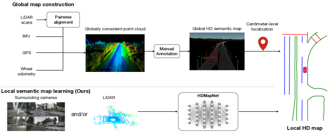
We propose a semantic map learning method named HDMapNet, which produces vectorized map elements from images of the surrounding cameras and/or from point clouds like LiDARs. We study how to effectively transform perspective image features to bird’s-eye view features when depth is missing. We put forward a novel view transformer that consists of both neural feature transformation and geometric projection. Moreover, we investigate whether point clouds and camera images complement each other in this task. We find different map elements are not equally recognizable in a single modality. To take the best from both worlds, our best model combines point cloud representations with image representations. This model outperforms its single-modal counterparts by a significant margin in all categories. To demonstrate the practical value of our method, we generate a locally-consistent map using our model in Figure 6; the map is immediately applicable to real-time motion planning.

Finally, we propose comprehensive ways to evaluate the performance of map learning. These metrics include both semantic level and instance level evaluations as map elements are typically represented as object instances in HD maps. On the public NuScenes dataset, HDMapNet improves over existing methods by 12.1 IoU on semantic segmentation and 13.1 mAP on instance detection.

To summarize, our contributions include the following:

• We propose a novel online framework to construct HD semantic maps from the sensory observations, and together with a method named HDMapNet.

• We come up with a novel feature projection module from perspective view to bird’s-eye view. This module models 3D environments implicitly and considers the camera extrinsic explicitly.

• We develop comprehensive evaluation protocols and metrics to facilitate future research.

II Related Work

Semantic map construction. Most existing HD semantic maps are annotated either manually or semi-automatically on LiDAR point clouds of the environment, merged from LiDAR scans collected from survey vehicles with high-end GPS and IMU. SLAM algorithms are the most commonly used algorithms to fuse LiDAR scans into a highly accurate and consistent point cloud. First, pairwise alignment algorithm like ICP [1], NDT [2] and their variants [3] are employed to match LiDAR data at two nearby timestamps using semantic [4] or geometry information [5]. Second, estimating accurate poses of ego vehicle is formulated as a non-linear least-square problem [6] or a factor graph [7] which is critical to build a globally consistent map. Yang et al. [8] presented a method for reconstructing maps at city scale based on the pose graph optimization under the constraint of pairwise alignment factor. To reduce the cost of manual annotation of semantic maps, [9, 10] proposed several machine learning techniques to extract static elements from fused LiDAR point clouds and cameras. However, it is still laborious and costly to maintain an HD semantic map since it requires high precision and timely update. In this paper, we argue that our proposed local semantic map learning task is a potentially more scalable solution for autonomous driving.

Perspective view lane detection. The traditional perspective-view-based lane detection pipeline involves local image feature extraction (e.g. color, directional filters [11, 12, 13]) , line fitting (e.g. Hough transform [14]), image-to-world projection, etc. With the advances of deep learning based image segmentation and detection techniques [15, 16, 17, 18], researchers have explored more data-driven approaches. Deep models were developed for road segmentation [19, 20], lane detection [21, 22], drivable area analysis [23], etc. More recently, models were built to give 3D outputs rather than 2D. Bai et al. [24] incorporated LiDAR signals so that image pixels can be projected onto the ground. Garnett et al. [25] and Guo et al. [26] used synthetic lane datasets to perform supervised training on the prediction of camera height and pitch, so that the output lanes sit in a 3D ground plane. Beyond detecting lanes, our work outputs a consistent local semantic map around the vehicle from surround cameras or LiDARs.

Cross-view learning. Recently, some efforts have been made to study cross-view learning to facilitate robots’ surrounding sensing capability. Pan [27] used MLPs to learn the relationship between perspective-view feature maps and bird’s-eye view feature maps. Roddick and Cipolla [28] applied 1D convolution on the image fetures along the horizontal axis to predict bird’s-eye view. Philion and Fidler [29] predicted the depth of monocular cameras and project image features into bird’s-eye view using soft attention. Our work focuses on the crucial task of local semantic map construction that we use cross-view sensing methods to generate map elements in a vectorized form. Moreover, our model can be easily fused with LiDAR input to further improve its accuracy.

III Semantic Map Learning

We propose semantic map learning, a novel framework that produces local high-definition semantic maps. It takes sensor inputs like camera images and LiDAR point clouds, and outputs vectorized map elements, such as lane dividers, lane boundaries and pedestrian crossings. We use $ℐ$ and $P$ to denote the images and point clouds, respectively. Optionally, the framework can be extended to include other sensor signals like radars. We define $ℳ$ as the map elements to predict.

III-A HDMapNet

Figure 2: Model overview. HDMapNet works with either or both of images and point clouds, outputs semantic segmentation, instance embedding and directions, and finally produces a vectorized local semantic map. Top left: image branch. Bottom left: point cloud branch. Right: HD semantic map. .

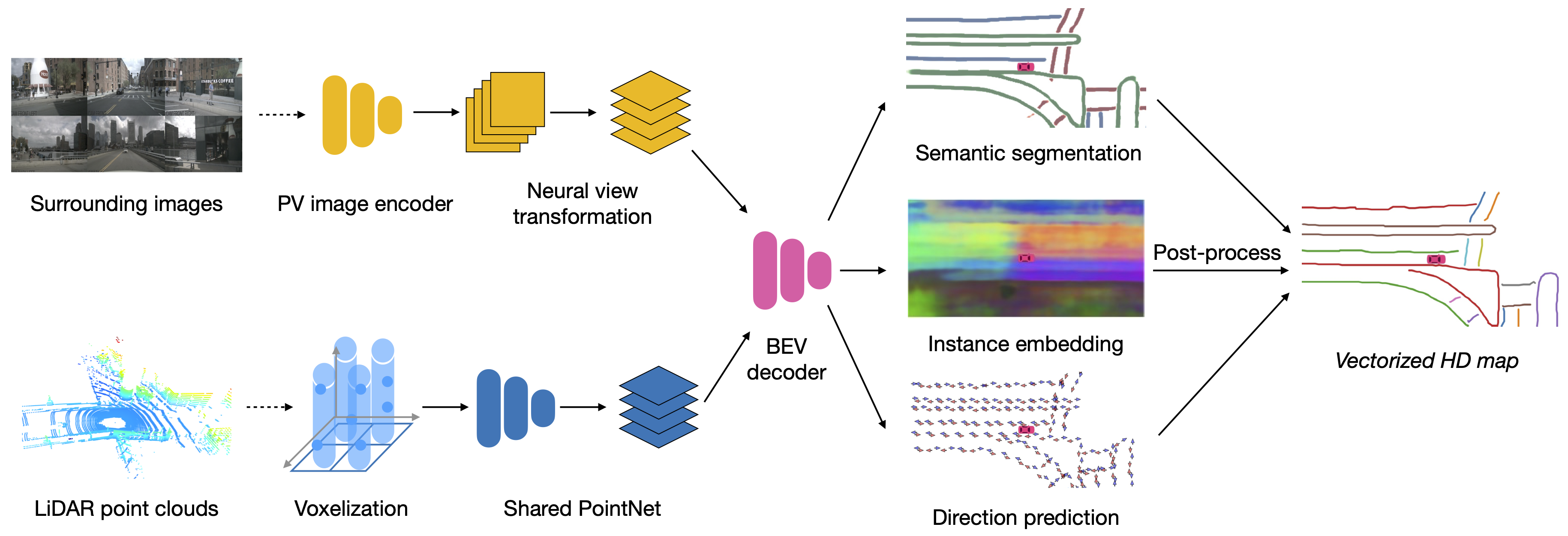
Our semantic map learning model, named HDMapNet, predicts map elements $ℳ$ from single frame $ℐ$ and $P$ with neural networks directly. An overview is shown in Figure 2, four neural networks parameterize our model: a perspective view image encoder ${\varphi }_{ℐ}$ and a neural view transformer ${\varphi }_{𝒱}$ in the image branch, a pillar-based point cloud encoder ${\varphi }_P$, and a map element decoder ${\varphi }_{ℳ}$. We denote our HDMapNet family as HDMapNet(Surr), HDMapNet(LiDAR), HDMapNet(Fusion) if the model takes only surrounding images, only LiDAR, or both of them as input.

III-A1 Image encoder

Our image encoder has two components, namely perspective view image encoder and neural view transformer.

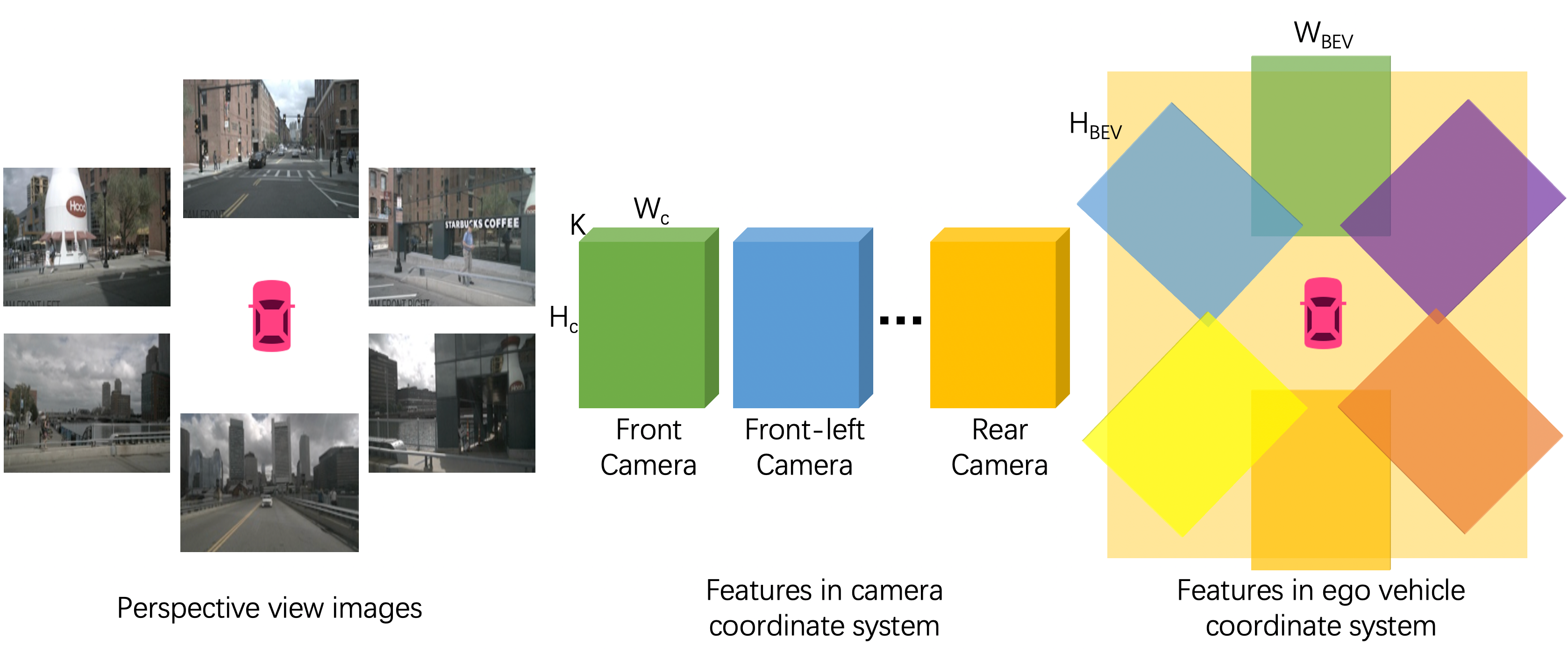
Perspective view image encoder. Our image branch takes perspective view inputs from $N_m$ surrounding cameras, covering the panorama of the scene. Each image ${ℐ}_i$ is embedded by a shared neural network ${\varphi }_{ℐ}$ to get perspective view feature map ${ℱ}_{{ℐ}_i}^{\mathrm{pv}}\subseteq {ℝ}^{H_{\mathrm{pv}}\times W_{\mathrm{pv}}\times K}$ where $H_{\mathrm{pv}}$, $W_{\mathrm{pv}}$, and $K$ are the height, width, and feature dimension respectively.

Neural view transformer. As shown in Figure 3, we first transform image features from perspective view to camera coordinate system and then to bird’s-eye view. The relation of any two pixels between perspective view and camera coodinate system is modeled by a multi-layer perceptron ${\varphi }_{{𝒱}_i}$:

$${ℱ}_{{ℐ}_i}^c[h][w]={\varphi }_{{𝒱}_i}^{hw}({ℱ}_{{ℐ}_i}^{\mathrm{pv}}[1][1],\mathrm{\dots },{ℱ}_{{ℐ}_i}^{\mathrm{pv}}[H_{\mathrm{pv}}][W_{\mathrm{pv}}])$$ (1)

where ${\varphi }_{{𝒱}_i}^{hw}$ models the relation between feature vector at position $(h,w)$ in the camera coodinate system and every pixel on the perspective view feature map. We denote $H_c$ and $W_c$ as the top-down spatial dimensions of $F_{ℐ}^c$. The bird’s-eye view (ego coordinate system) features ${ℱ}_{{ℐ}_i}^{\mathrm{bev}}\subseteq {ℝ}^{H_{\mathrm{bev}}\times W_{\mathrm{bev}}\times K}$ is obtained by transforming the features ${ℱ}_{{ℐ}_i}^c$ using geometric projection with camera extrinsics, where $H_{\mathrm{bev}}$ and $W_{\mathrm{bev}}$ are the height and width in the bird’s-eye view. The final image feature ${ℱ}_{ℐ}^{\mathrm{bev}}$ is an average of $N_m$ camera features.

III-A2 Point cloud encoder

Our point cloud encoder ${\varphi }_P$ is a variant of PointPillar [30] with dynamic voxelization [31], which divide the 3d space into multiple pillars and learn feature maps from pillar-wise features of pillar-wise point clouds. The input is $N$ lidar points in the point cloud. For each point $p$, it has three-dimensional coordinates and additional $K$-dimensional features represented as $f_p\subseteq {ℝ}^{K+3}$.

When projecting features from points to bird’s-eye view, multiple points can potentially fall into the same pillar. We define $P_j$ as the set of points corresponding to pillar $j$. To aggregate features from points in a pillar, a PointNet [32] (denoted as $\mathrm{PN}$) is warranted, where

$$\begin{array}{c}\hfill f_j^{\mathrm{pillar}}=\mathrm{PN}(\{f_p|\forall p\in P_j\}).\end{array}$$ (2)

Then, pillar-wise features are further encoded through a convolutional neural network ${\varphi }_{\mathrm{pillar}}$. We denote the feature map in the bird’s-eye view as ${ℱ}_P^{\mathrm{bev}}$.

III-A3 Bird’s-eye view decoder

The map is a complex graph network that includes instance-level and directional information of lane dividers and lane boundaries. Instead of pixel-level representation, lane lines need to be vectorized so that they can be followed by self-driving vehicles. Therefore, our BEV decoder ${\varphi }_{ℳ}$ not only outputs semantic segmentation but also predicts instance embedding and lane direction. A post-processing process is applied to cluster instances from embeddings and vectorize them.

Overall architecture. The BEV decoder is a fully convolutional network (FCN) [33] with 3 branches, namely semantic segmentation branch, instance embedding branch, and direction prediction branch. The input of BEV decoder is image feature map $F_{ℐ}^{\mathrm{bev}}$ and/or point cloud feature map $F_P^{\mathrm{bev}}$, and we concatenate them if both exist.

Semantic prediction. The semantic prediction module is a fully convolutional network (FCN) [33] We use cross-entropy loss for the semantic prediction.

Instance embedding. Our instance embedding module seeks to cluster each bird’s-eye view embedding. For ease of notation, we follow the exact definition in [34]: $C$ is the number of clusters in the ground truth, $N_c$ is the number of elements in cluster $c$, ${\mu }_c$ is the mean embedding of cluster c, $\parallel \cdot \parallel$ is the L2 norm, and ${[x]}_{+}$ = max(0, x) denotes the element maximum. ${\delta }_v$ and ${\delta }_d$ are respectively the margins for the variance and distance loss. The clustering loss $L$ is computed by:

$L_{var}={\displaystyle \frac{1}{C}}{\displaystyle \sum _{c=1}^C}{\displaystyle \frac{1}{N_c}}{\displaystyle \sum _{j=1}^{N_c}}{[\Vert {\mu }_c-f_j^{\mathrm{instance}}\Vert -{\delta }_v]}_{+}^2$ (3)

$L_{dist}={\displaystyle \frac{1}{C(C-1)}}{\displaystyle \sum _{c_A\ne c_B\in C}}{[2{\delta }_d-\Vert {\mu }_{c_A}-{\mu }_{c_B}\Vert ]}_{+}^2,$ (4)

$L=\alpha L_{var}+\beta L_{dist}.$ (5)

Figure 3: Feature transformation. Left: the 6 input images in the perspective view. Middle: 6 feature maps in camera coordinate system, which are obtained by extracting features using image encoder and transforming these features with MLP; each feature map (in different colors) covers a certain area. Right: the feature map (in orange) in the ego vehicle coordinate system; this is fused from 6 feature maps and transformed to the ego vehicle coordinate system with camera extrinsics.

Direction prediction. Our direction module aims to predict directions of lanes from each pixel $C$. The directions are discretized into $N_d$ classes uniformed distributed on a unit circle. By classifying direction $D$ of current pixel $C_{now}$, the next pixel of lane $C_{next}$ can be obtained as $C_{next}=C_{now}+{\mathrm{\Delta }}_{step}\cdot D$, where ${\mathrm{\Delta }}_{step}$ is a predefined step size. Since we don’t know the direction of the lane, we cannot identify the forward and backward direction of each node. Instead, we treat both of them as positive labels. Concretely, the direction label of each lane node is a $N_d$ vector with 2 indices labeled as 1 and others labeled as 0. Note that most of the pixels on the topdown map don’t lie on the lanes, which means they don’t have directions. The direction vector of those pixels is a zero vector and we never do backpropagation for those pixels during training. We use softmax as the activation function for classification.

Ground Truth

IPM

IPM(B)

IPM(CB)

Lift-Splat-Shoot

VPN

HDMapNet(Surr)

HDMapNet(LiDAR)

HDMapNet(Fusion)

Figure 4: Qualitative results on the validation set. Top left: the surrounding images and the ground-truth local semantic map annotations. IPM: the lane segmentation result in the perspective view and the bird’s-eye view. Others: the semantic segmentation results and the vectorized instance detection results.

Vectorization. During inference, we first cluster instance embeddings using the Density-Based Spatial Clustering of Applications with Noise (DBSCAN). Then non-maximum suppression (NMS) is used to reduce redundancy. Finally, the vector representations are obtained by greedily connecting the pixels with the help of the predicted direction.

III-B Evaluation

In this section, we propose evaluation protocols for semantic map learning, including semantic metrics and instance metrics.

III-B1 Semantic metrics

The semantics of model predictions can be evaluated in the Eulerian fashion and the Lagrangian fashion. Eulerian metrics are computed on a dense grid and measure the pixel value differences. In contrast, Lagrangian metrics move with the shape and measure the spatial distances of shapes.

Eulerian metrics. We use intersection-over-union (IoU) as Eulerian metrics, which is given by,

$$\mathrm{IoU}({𝒟}_1,{𝒟}_2)=\frac{|{𝒟}_1\cap {𝒟}_2|}{|{𝒟}_1\cup {𝒟}_2|},$$ (6)

where ${𝒟}_1,{𝒟}_2\subseteq {ℝ}^{H\times W\times D}$ are dense representations of shapes (curves rasterized on a grid); $H$ and $W$ are the height and width of the grid, $D$ is number of categories; $|\cdot |$ denotes the size of the set.

Lagrangian metrics. We are interested in structured outputs, namely curves consists of connected points. To evaluate the spatial distances between the predicted curves and ground-truth curves, we use Chamfer distance (CD) of between point sets sampled on the curves:

${\mathrm{CD}}_{\mathrm{Dir}}({𝒮}_1,{𝒮}_2)={\displaystyle \frac{1}{{𝒮}_1}}{\displaystyle \sum _{x\in {𝒮}_1}}\underset{y\in {𝒮}_2}{\min }{\Vert x-y\Vert }_2$ (7)

$\mathrm{CD}({𝒮}_1,{𝒮}_2)={\mathrm{CD}}_{\mathrm{Dir}}({𝒮}_1,{𝒮}_2)+{\mathrm{CD}}_{\mathrm{Dir}}({𝒮}_2,{𝒮}_1)$ (8)

where ${\mathrm{CD}}_{\mathrm{dir}}$ is the directional Chamfer distance and $\mathrm{CD}$ is the bi-directional Chamfer distance; ${𝒮}_1$ and ${𝒮}_2$ are the two sets of points on the curves.

III-B2 Instance metrics

We further evaluate the instance detection capability of our models. We use average precision (AP) similar to the one in object detection [35], given by

$$\mathrm{AP}=\frac{1}{10}\sum _{r\in \{0.1,0.2,\mathrm{\dots },1.0\}}{\mathrm{AP}}_r,$$ (9)

where ${\mathrm{AP}}_r$ is the precision at recall=$r$. We collect all predictions and rank them in descending order according to the semantic confidences. Then, we classify each prediction based on the CD threshold. For example, if the CD is lower than a predefined threshold, it is considered true positive, otherwise false positive. Finally, we obtain all precision-recall pairs and compute APs accordingly.

IV Experiments

IV-A Implementation details

Tasks & Metrics. We evaluate our approach on the NuScenes dataset [36]. We focus on two sub-tasks: semantic map segmentation and instance detection. Due to the limited types of map elements in the nuScenes dataset, we consider three static map elements: lane boundary, lane divider, and pedestrian crossing.

Architecture. For the perspective view image encoder, we adopt EfficientNet-B0 [37] pre-trained on ImageNet [38], as in [29]. Then, we use a multi-layer perceptron (MLP) to convert the perspective view features to bird’s-eye view features in the camera coordinate system. The MLP is shared channel-wisely and does not change the feature dimension. For point clouds, we use a variant of PointPillars [39] with dynamic voxelization [31]. We use a PointNet [32] with a 64-dimensional layer to aggregate points in a pillar. ResNet [40] with three blocks is used as the BEV decoder.

Training details. We use the cross-entropy loss for the semantic segmentation, and use the discriminative loss (Equation 5) for the instance embedding where we set $\alpha =\beta =1$, ${\delta }_v=0.5$, and ${\delta }_d=3.0$. We use Adam [41] for model training, witfh a learning rate of $1e-3$.

IV-B Baseline methods

TABLE I: IoU scores (%) and CD (m) of semantic map segmentation. CD_P denotes the CD from label to prediction (equivalent to precision) while CD_L denotes the CD from Prediction to Label (equivalent to recall); CD is the average of them. IoU: higher is better. CD: lower is better. *: the perspective view labels projected from 2D HD Maps.

Method	Divider				Ped Crossing				Boundary				All Classes
	IoU	CDP	CDL	CD	IoU	CDP	CDL	CD	IoU	CDP	CDL	CD	IoU	CDP	CDL	CD
IPM∗	14.4	1.149	2.232	2.193	9.5	1.232	3.432	2.482	18.4	1.502	2.569	1.849	14.1	1.294	2.744	2.175
IPM(B)	25.5	1.091	1.730	1.226	12.1	0.918	2.947	1.628	27.1	0.710	1.670	0.918	21.6	0.906	2.116	1.257
IPM(CB)	38.6	0.743	1.106	0.802	19.3	0.741	2.154	1.081	39.3	0.563	1.000	0.633	32.4	0.682	1.42	0.839
Lift-Splat-Shoot [29]	38.3	0.872	1.144	0.916	14.9	0.680	2.691	1.313	39.3	0.580	1.137	0.676	30.8	0.711	1.657	0.968
VPN [27]	36.5	0.534	1.197	0.919	15.8	0.491	2.824	2.245	35.6	0.283	1.234	0.848	29.3	0.436	1.752	1.337
HDMapNet(Surr)	40.6	0.761	0.979	0.779	18.7	0.855	1.997	1.101	39.5	0.608	0.825	0.624	32.9	0.741	1.267	0.834
HDMapNet(LiDAR)	26.7	1.134	1.508	1.219	17.3	1.038	2.573	1.524	44.6	0.501	0.843	0.561	29.5	0.891	1.641	1.101
HDMapNet(Fusion)	46.1	0.625	0.893	0.667	31.4	0.535	1.715	0.790	56.0	0.461	0.443	0.459	44.5	0.540	1.017	0.639

For all baseline methods, we use the same image encoder and decoder as HDMapNet and only change the view transformation module.

Inverse Perspective Mapping (IPM). The most straightforward baseline is to map segmentation predictions to the bird’s-eye view via IPM [42, 43].

IPM with bird’s-eye view decoder (IPM(B)). Our second baseline is an extension of IPM. Rather than making predictions in perspective view, we perform semantic segmentation directly in bird-eye view.

IPM with perspective view feature encoder and bird’s-eye view decoder (IPM(CB)). The next extension is to perform feature learning in the perspective view while making predictions in the bird’s-eye view.

Lift-Splat-Shoot. Lift-Splat-Shoot [29] estimates a distribution over depth in the perspective view images. Then, it converts 2D images into 3D point clouds with features and projects them into the ego vehicle frame.

View Parsing Network (VPN). VPN [27] proposes a simple view transformation module: a view relation module to model the relations between any two pixels and a view fusion module to fuses the features of pixels.

TABLE II: Instance detection results. {0.2, 0.5, 1.} are the predefined thresholds of Chamfer distance (e.g. a prediction is considered a true positive if the Chamfer distance between label and prediction is lower than that threshold). The mAP is the average of three APs. AP & mAP: higher is better.

Method	Divider				Ped Crossing				Boundary				All Classes
	AP@.2	AP@.5	AP@1.	mAP	AP@.2	AP@.5	AP@1.	mAP	AP@.2	AP@.5	AP@1.	mAP	AP@.2	AP@.5	AP@1.	mAP
IPM(B)	2.6	9.8	19.6	10.7	1.6	4.8	7.8	4.7	2.2	9.2	23.7	11.7	2.1	7.9	17.0	9.0
IPM(CB)	10.2	25.0	36.8	24.0	2.0	7.8	12.2	7.3	10.1	27.9	45.5	27.8	7.4	20.2	31.5	19.7
Lift-Splat-Shoot [29]	9.1	23.8	35.9	22.9	0.9	5.4	8.9	5.1	8.5	22.9	41.2	24.2	6.2	17.4	28.7	17.4
VPN [27]	8.8	22.7	34.9	22.1	1.2	5.3	9.0	5.2	9.2	24.1	42.7	25.3	6.4	17.4	28.9	17.5
HDMapNet(Surr)	13.7	30.7	40.6	28.3	1.9	7.4	12.1	7.1	13.7	33.9	50.1	32.6	9.8	24.0	34.3	22.7
HDMapNet(LiDAR)	1.0	5.7	15.1	7.3	1.9	5.8	9.0	5.6	5.8	20.2	39.6	21.9	2.9	10.6	21.2	11.6
HDMapNet(Fusion)	15.0	32.6	46.0	31.2	6.4	13.6	17.8	12.6	26.7	51.5	65.6	47.9	16.0	32.6	43.1	30.6

Figure 5: Qualitative results under bad weather conditions. The left two images show predictions at night. The right twos show predictions at rainy days.

IV-C Results

We compare our HDMapNet against baselines in Section IV-B. Table I shows the comparisons. First, Our HDMapNet(Surr), which is the surrounding camera-only method, outperforms all baselines. This suggests that our novel learning-based view transformation is indeed effective, without making impractical assumptions about a complex ground plane (IPM) or estimating the depth (Lift-Splat-Shoot). Second, our HDMapNet(LiDAR) is better than HDMapNet(Surr) in boundary but worse in divider and pedestrian crossing. This indicates different categories are not equally recognizable in one modality. Third, our fusion model with both camera images and LiDAR point clouds achieves the best performance. It improves over baselines and our camera-only method by 50% relatively.

Another interesting phenomenon is that various models behave differently in terms of the CD. For example, VPN has the lowest CD_P in all categories, while it underperforms its counterparts on CD_L and has the worst overall CD. Instead, our HDMapNet(Surr) balances both CD_P and CD_L, achieving the best CD among all camera-only-based methods. This finding indicates that CD is complementary to IoU, which shows the precision and recall aspects of models. This helps us understand the behaviors of different models from another perspective.

Figure 6: Long-term temporal accumulation by fusing occupancy probabilities over multiple frames.

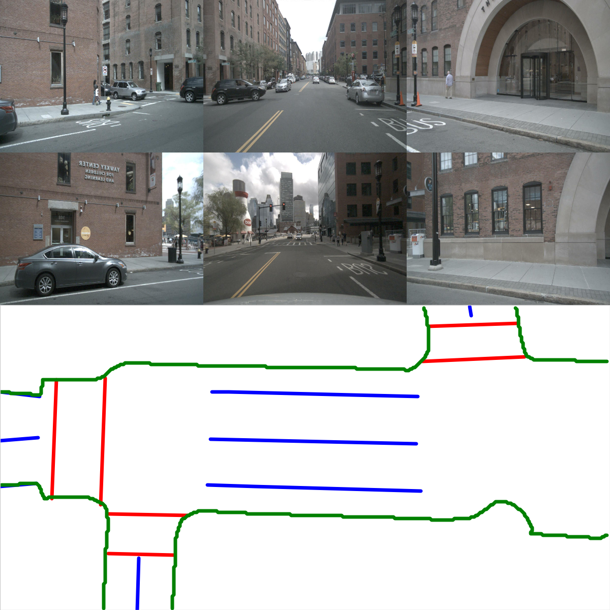
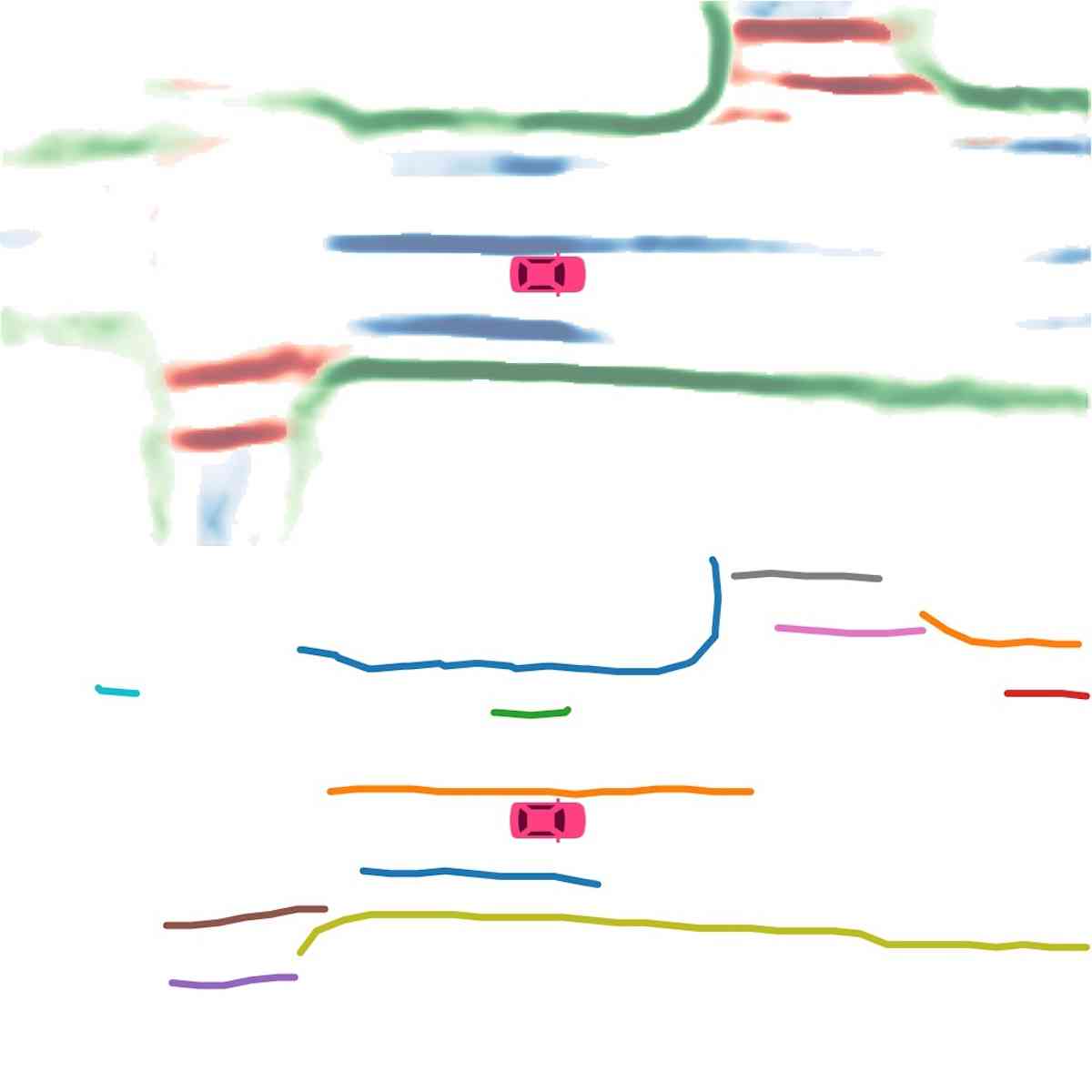
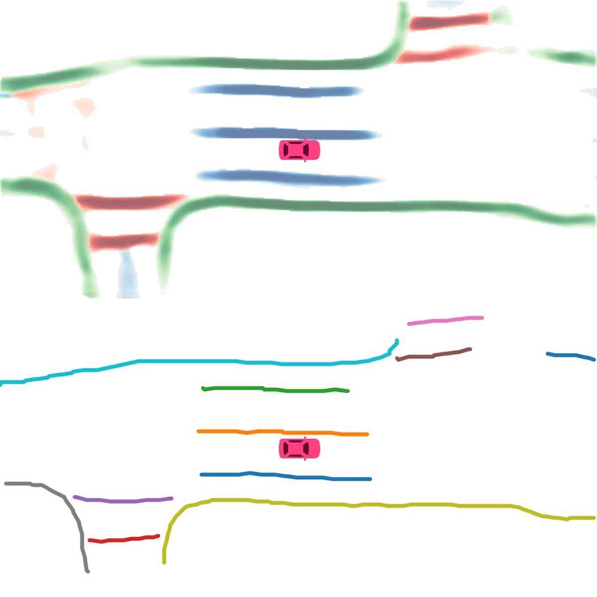
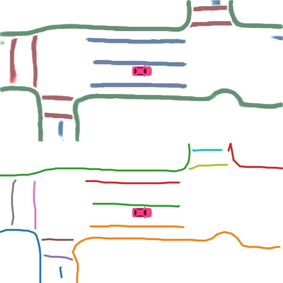
Instance map detection. In Figure 2 (Instance detection branch), we show the visualization of embeddings using principal component analysis (PCA). Different lanes are assigned different colors even when they are close to each other or have intersections. This confirms our model learns instance-level information and can predict instance labels accurately. In Figure 2 (Direction classification branch), we show the direction mask predicted by our direction branch. The direction is consistent and smooth. We show the vectorized curve produced after post processing in Figure 4. In Table II, we present the quantitative results of instance map detection. HDMapNet(Surr) already outperforms baselines while HDMapNet(Fusion) is significantly better than all counterparts, e.g., it improves over IPM by 55.4%.

Sensor fusion. In this section, we further analyze the effect of sensor fusion for constructing HD semantic maps. As shown in Table I, for divider and pedestrian crossing, HDMapNet(Surr) outperforms HDMapNet(LiDAR), while for lane boundary, HDMapNet(LiDAR) works better. We hypothesize this is because there are elevation changes near the lane boundary, making it easy to detect in LiDAR point clouds. On the other hand, the color contrast of road divider and pedestrian crossing is helpful information, making two categories more recognizable in images; visualizations also confirm this in Figure 4. The strongest performance is achieved when combining LiDAR and cameras; the combined model outperforms both models with a single sensor by a large margin. This suggests these two sensors include complementary information for each other.

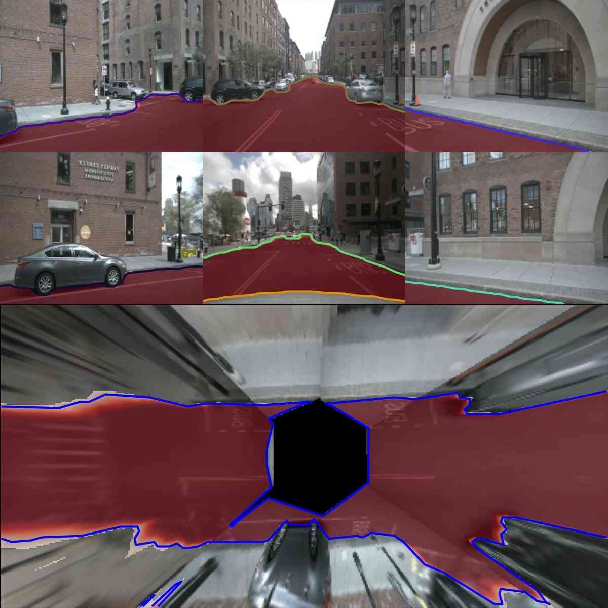
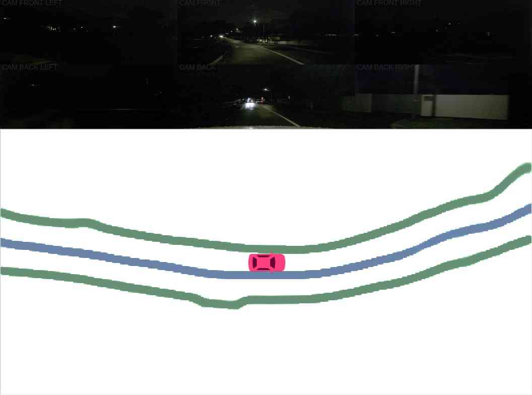
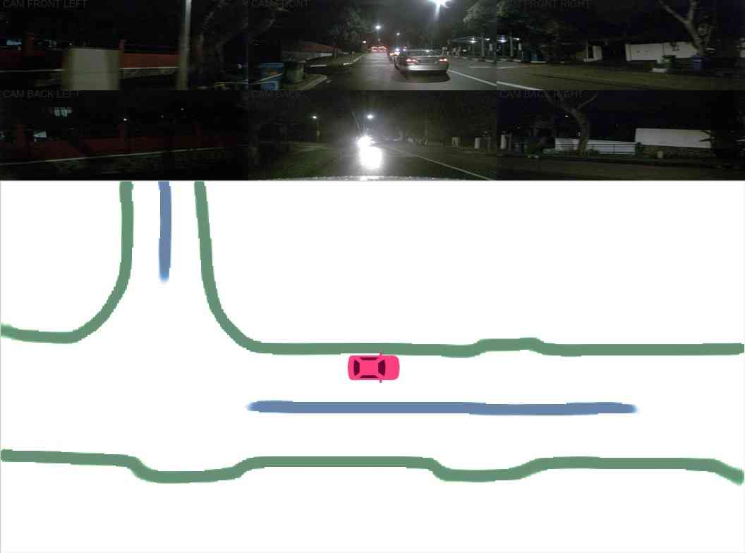
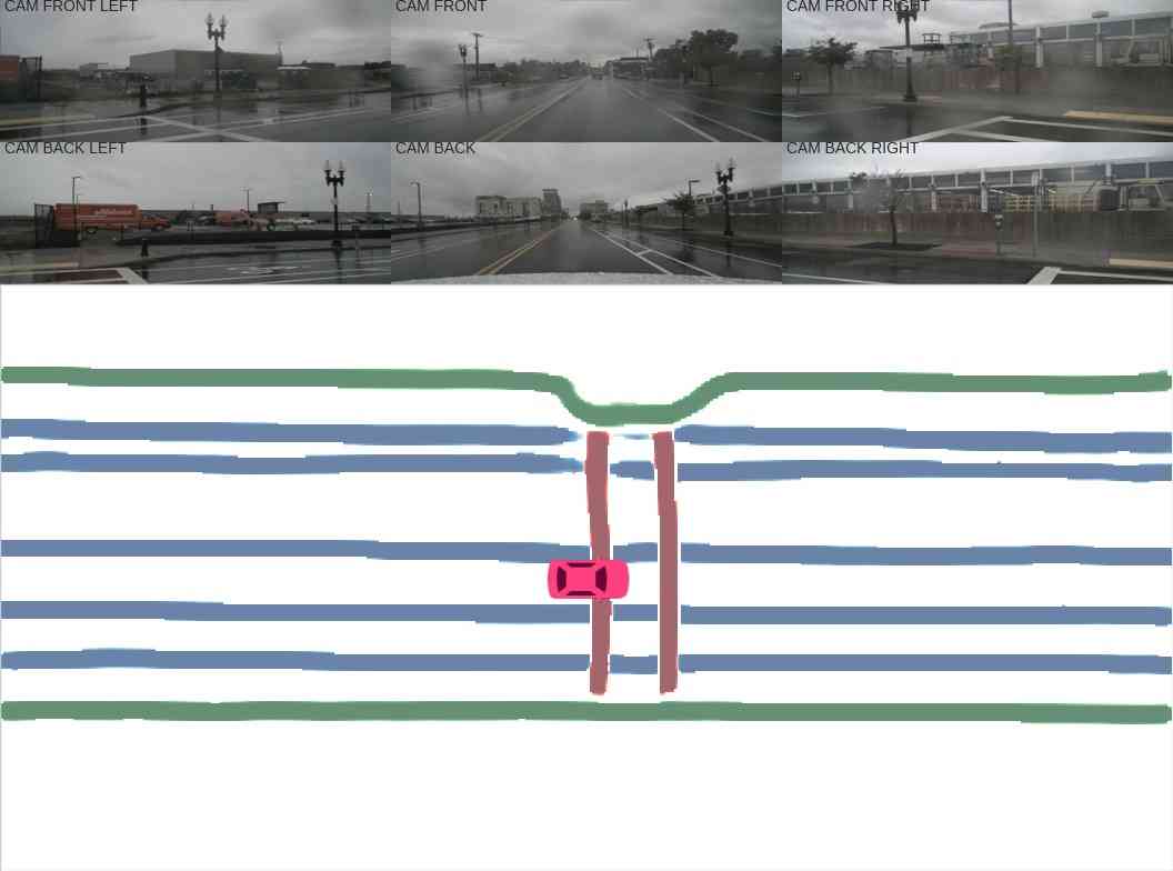
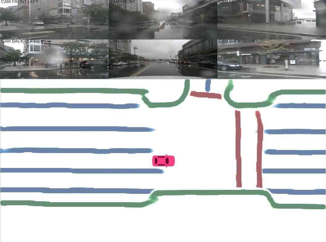
Bad weather conditions. Here we assess the robustness of our model under extreme weather conditions. As shown in Figure 5, our model can generate complete lanes even when lighting condition is bad, or when the rain obscures sight. We speculate that the model can predict the shape of the lane based on partial observations when the roads are not completely visible. Although there are performance drop in extreme weather condition, the overall performance is still reasonable. (Table III)

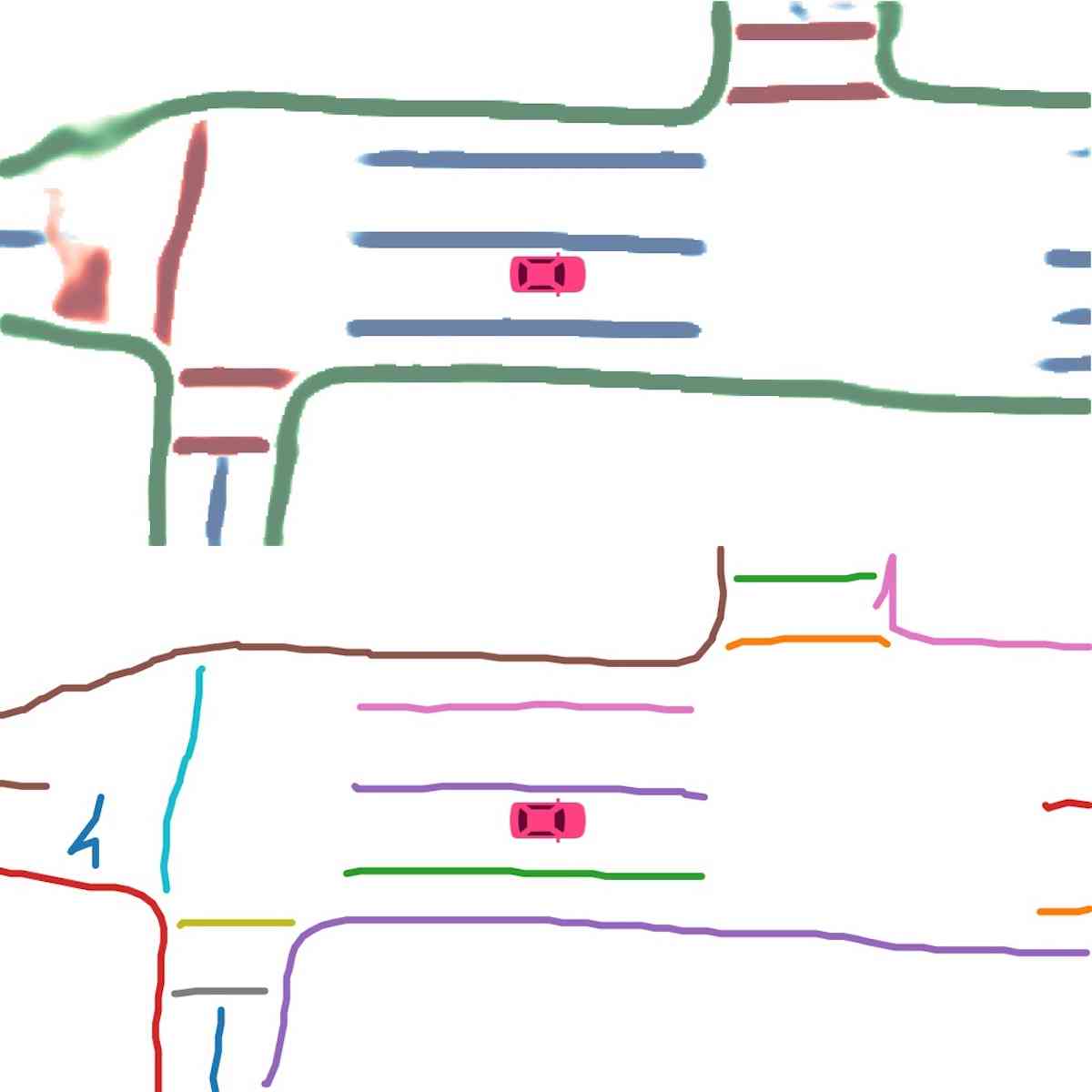
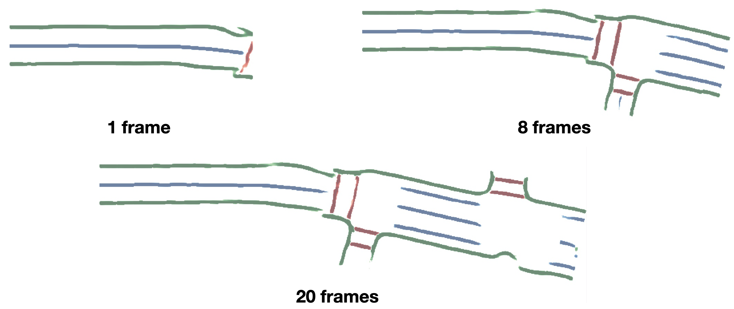
Temporal Fusion. Here we experiment on temporal fusion strategies. We first conduct short-term temporal fusion by pasting feature maps of previous frames into current’s according to ego poses. The feature maps are fused by max pooling and then fed into decoder. As shown in Table IV, fusing multiple frames can improve the IoU of the semantics. We further experiment on long-term temporal accumulation by fusing segmentation probabilities. As shown in Figure 6, our method produces consistent semantic maps with larger field of view while fusing multiple frames.

Weather	Night	Rainy	Normal
IoU	39.3	38.7	44.9

TABLE III: The semantic segmentation performance of HDMapNet(Fusion) under different weather.

# of frames	1	2	4
IoU	32.9	35.8	36.4

TABLE IV: Temporal fusion on HDMapNet(Surr). 1 means temporal fusion is not used.

V Conclusion

HDMapNet predicts HD semantic maps directly from camera images and/or LiDAR point clouds. The local semantic map learning framework could be a more scalable approach than the global map construction and annotation pipeline that requires a significant amount of human efforts. Even though our baseline method of semantic map learning does not produce map elements as accurate, it gives system developers another possible choice of the trade-off between scalability and accuracy.

References

- [1] P. J. Besl and N. D. McKay, “Method for registration of 3-d shapes,” in Sensor fusion IV: control paradigms and data structures, vol. 1611. International Society for Optics and Photonics, 1992, pp. 586–606.
- [2] P. Biber and W. Straßer, “The normal distributions transform: A new approach to laser scan matching,” in Proceedings 2003 IEEE/RSJ International Conference on Intelligent Robots and Systems (IROS 2003)(Cat. No. 03CH37453), vol. 3. IEEE, 2003, pp. 2743–2748.
- [3] A. Segal, D. Haehnel, and S. Thrun, “Generalized-icp.” in Robotics: science and systems, vol. 2, no. 4. Seattle, WA, 2009, p. 435.
- [4] F. Yu, J. Xiao, and T. Funkhouser, “Semantic alignment of lidar data at city scale,” in Proceedings of the IEEE Conference on Computer Vision and Pattern Recognition, 2015, pp. 1722–1731.
- [5] F. Pomerleau, F. Colas, and R. Siegwart, “A review of point cloud registration algorithms for mobile robotics,” Foundations and Trends in Robotics, vol. 4, no. 1, pp. 1–104, 2015.
- [6] C. L. Lawson and R. J. Hanson, Solving least squares problems. SIAM, 1995.
- [7] F. Dellaert, “Factor graphs and gtsam: A hands-on introduction,” Georgia Institute of Technology, Tech. Rep., 2012.
- [8] S. Yang, X. Zhu, X. Nian, L. Feng, X. Qu, and T. Ma, “A robust pose graph approach for city scale lidar mapping,” in 2018 IEEE/RSJ International Conference on Intelligent Robots and Systems (IROS). IEEE, 2018, pp. 1175–1182.
- [9] J. Jiao, “Machine learning assisted high-definition map creation,” in 2018 IEEE 42nd Annual Computer Software and Applications Conference (COMPSAC), vol. 1. IEEE, 2018, pp. 367–373.
- [10] L. Mi, H. Zhao, C. Nash, X. Jin, J. Gao, C. Sun, C. Schmid, N. Shavit, Y. Chai, and D. Anguelov, “Hdmapgen: A hierarchical graph generative model of high definition maps,” in Proceedings of the IEEE/CVF Conference on Computer Vision and Pattern Recognition (CVPR), June 2021, pp. 4227–4236.
- [11] K.-Y. Chiu and S.-F. Lin, “Lane detection using color-based segmentation,” in IEEE Proceedings. Intelligent Vehicles Symposium, 2005. IEEE, 2005, pp. 706–711.
- [12] H. Loose, U. Franke, and C. Stiller, “Kalman particle filter for lane recognition on rural roads,” in 2009 IEEE Intelligent Vehicles Symposium. IEEE, 2009, pp. 60–65.
- [13] S. Zhou, Y. Jiang, J. Xi, J. Gong, G. Xiong, and H. Chen, “A novel lane detection based on geometrical model and gabor filter,” in 2010 IEEE Intelligent Vehicles Symposium. IEEE, 2010, pp. 59–64.
- [14] J. Illingworth and J. Kittler, “A survey of the hough transform,” Computer vision, graphics, and image processing, vol. 44, no. 1, pp. 87–116, 1988.
- [15] J. M. Alvarez, T. Gevers, Y. LeCun, and A. M. Lopez, “Road scene segmentation from a single image,” in ECCV, 2012.
- [16] B. Zhou, H. Zhao, X. Puig, S. Fidler, A. Barriuso, and A. Torralba, “Scene parsing through ade20k dataset,” in Proceedings of the IEEE conference on computer vision and pattern recognition, 2017, pp. 633–641.
- [17] A. Ess, T. Mueller, H. Grabner, and L. Van Gool, “Segmentation-based urban traffic scene understanding.” in BMVC, vol. 1. Citeseer, 2009, p. 2.
- [18] M. Cordts, M. Omran, S. Ramos, T. Rehfeld, M. Enzweiler, R. Benenson, U. Franke, S. Roth, and B. Schiele, “The cityscapes dataset for semantic urban scene understanding,” in CVPR, 2016.
- [19] F. Yu, W. Xian, Y. Chen, F. Liu, M. Liao, V. Madhavan, and T. Darrell, “Bdd100k: A diverse driving video database with scalable annotation tooling,” arXiv preprint arXiv:1805.04687, vol. 2, no. 5, p. 6, 2018.
- [20] G. Neuhold, T. Ollmann, S. Rota Bulo, and P. Kontschieder, “The mapillary vistas dataset for semantic understanding of street scenes,” in Proceedings of the IEEE International Conference on Computer Vision, 2017, pp. 4990–4999.
- [21] Z. Wang, W. Ren, and Q. Qiu, “Lanenet: Real-time lane detection networks for autonomous driving,” arXiv preprint arXiv:1807.01726, 2018.
- [22] D. Neven, B. De Brabandere, S. Georgoulis, M. Proesmans, and L. Van Gool, “Towards end-to-end lane detection: an instance segmentation approach,” in 2018 IEEE intelligent vehicles symposium (IV). IEEE, 2018, pp. 286–291.
- [23] X. Liu and Z. Deng, “Segmentation of drivable road using deep fully convolutional residual network with pyramid pooling,” Cognitive Computation, vol. 10, no. 2, pp. 272–281, 2018.
- [24] M. Bai, G. Mattyus, N. Homayounfar, S. Wang, K. Lakshmikanth, Shrinidhi, and R. Urtasun, “Deep multi-sensor lane detection,” in IROS, 2018.
- [25] N. Garnett, R. Cohen, T. Pe’er, R. Lahav, and D. Levi, “3d-lanenet: end-to-end 3d multiple lane detection,” in Proceedings of the IEEE/CVF International Conference on Computer Vision, 2019, pp. 2921–2930.
- [26] Y. Guo, G. Chen, P. Zhao, W. Zhang, J. Miao, J. Wang, and T. E. Choe, “Genlanenet: A generalized and scalable approach for 3d lane detection,” 2020.
- [27] B. Pan, J. Sun, H. Y. T. Leung, A. Andonian, and B. Zhou, “Cross-view semantic segmentation for sensing surroundings,” IEEE Robotics and Automation Letters, vol. 5, no. 3, p. 4867–4873, Jul 2020. [Online]. Available: http://dx.doi.org/10.1109/LRA.2020.3004325
- [28] T. Roddick and R. Cipolla, “Predicting semantic map representations from images using pyramid occupancy networks,” in Proceedings of the IEEE/CVF Conference on Computer Vision and Pattern Recognition, 2020, pp. 11 138–11 147.
- [29] J. Philion and S. Fidler, “Lift, splat, shoot: Encoding images from arbitrary camera rigs by implicitly unprojecting to 3d,” 2020.
- [30] A. H. Lang, S. Vora, H. Caesar, L. Zhou, J. Yang, and O. Beijbom, “Pointpillars: Fast encoders for object detection from point clouds,” in The IEEE Conference on Computer Vision and Pattern Recognition (CVPR), June 2019.
- [31] Y. Zhou, P. Sun, Y. Zhang, D. Anguelov, J. Gao, T. Ouyang, J. Guo, J. Ngiam, and V. Vasudevan, “End-to-end multi-view fusion for 3d object detection in LiDAR point clouds,” in The Conference on Robot Learning (CoRL), 2019.
- [32] C. R. Qi, H. Su, K. Mo, and L. J. Guibas, “Pointnet: Deep learning on point sets for 3d classification and segmentation,” in The IEEE Conference on Computer Vision and Pattern Recognition (CVPR), July 2017.
- [33] E. Shelhamer, J. Long, and T. Darrell, “Fully convolutional networks for semantic segmentation,” IEEE Transactions on Pattern Analysis and Machine Intelligence, vol. 39, no. 4, pp. 640–651, 2017.
- [34] B. De Brabandere, D. Neven, and L. Van Gool, “Semantic instance segmentation for autonomous driving,” in Proceedings of the IEEE Conference on Computer Vision and Pattern Recognition (CVPR) Workshops, July 2017.
- [35] T.-Y. Lin, M. Maire, S. Belongie, L. Bourdev, R. Girshick, J. Hays, P. Perona, D. Ramanan, C. L. Zitnick, and P. Dollár, “Microsoft coco: Common objects in context,” 2015.
- [36] H. Caesar, V. Bankiti, A. H. Lang, S. Vora, V. E. Liong, Q. Xu, A. Krishnan, Y. Pan, G. Baldan, and O. Beijbom, “nuscenes: A multimodal dataset for autonomous driving,” 2020.
- [37] M. Tan and Q. V. Le, “Efficientnet: Rethinking model scaling for convolutional neural networks,” 2020.
- [38] O. Russakovsky, J. Deng, H. Su, J. Krause, S. Satheesh, S. Ma, Z. Huang, A. Karpathy, A. Khosla, M. Bernstein, A. C. Berg, and L. Fei-Fei, “Imagenet large scale visual recognition challenge,” 2015.
- [39] A. H. Lang, S. Vora, H. Caesar, L. Zhou, J. Yang, and O. Beijbom, “Pointpillars: Fast encoders for object detection from point clouds,” 2019.
- [40] K. He, X. Zhang, S. Ren, and J. Sun, “Deep residual learning for image recognition,” in CVPR, 2016.
- [41] D. P. Kingma and J. Ba, “Adam: A method for stochastic optimization,” 2017.
- [42] L. Deng, M. Yang, H. Li, T. Li, B. Hu, and C. Wang, “Restricted deformable convolution-based road scene semantic segmentation using surround view cameras,” IEEE Transactions on Intelligent Transportation Systems, vol. 21, no. 10, p. 4350–4362, Oct 2020. [Online]. Available: http://dx.doi.org/10.1109/TITS.2019.2939832
- [43] T. Sämann, K. Amende, S. Milz, C. Witt, M. Simon, and J. Petzold, “Efficient semantic segmentation for visual bird’s-eye view interpretation,” 2018.