Distance-based detection of out-of-distribution silent failures for Covid-19 lung lesion segmentation

Abstract

Automatic segmentation of ground glass opacities and consolidations in chest computer tomography (CT) scans can potentially ease the burden of radiologists during times of high resource utilisation. However, deep learning models are not trusted in the clinical routine due to failing silently on out-of-distribution (OOD) data. We propose a lightweight OOD detection method that leverages the Mahalanobis distance in the feature space and seamlessly integrates into state-of-the-art segmentation pipelines. The simple approach can even augment pre-trained models with clinically relevant uncertainty quantification. We validate our method across four chest CT distribution shifts and two magnetic resonance imaging applications, namely segmentation of the hippocampus and the prostate. Our results show that the proposed method effectively detects far- and near-OOD samples across all explored scenarios.

1 Introduction

Automatic segmentation of lung lesions in chest computed tomography (CT) scans could standardise quantification and staging of pulmonary diseases such as Covid-19 and open the way for more effective utilisation of hospital resources. Ground glass opacities (GGOs) and consolidations are characteristic of pulmonary infections onset by the SARS-CoV-2 virus [45]. Since the early phases of the pandemic, many institutions have compiled scans from afflicted patients in intensive care, and some initiatives have publicly released cases with ground-truth delineations from expert thorax radiologists [51, 25, 44]. Deep learning has shown promising results in segmenting these patterns. Particularly the fully-automatic nnU-Net [24] secured top spots [18] (9 out of 10, including the first) in the leaderboard for the Covid-19 Lung CT Lesion Segmentation Challenge [51].

Unfortunately, models trained with publicly available cohorts may not generalise well to real-world clinical data, thus posing safety issues when deployed without extensive testing and/or quality assurance (QA) protocols. Deep learning models are known to fail for data that diverges from the training distribution [41]; a phenomenon commonly referred to as domain shift. This hinders the deployment of AI solutions during the Covid-19 pandemic [22], as most institutions do not dedicate resources to annotate in-house datasets. There are many potential causes for domain shift, ranging from changes in the acquisition process to naturally shifting patient populations. Some can unknowingly occur within the same institution, rendering even models trained with in-house data unreliable with the passage of time [53].

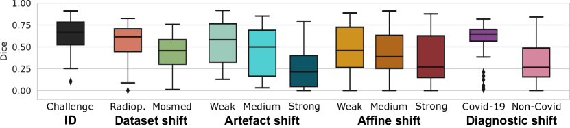
This performance deterioration is visualised in Figure 5 for an nnU-Net trained on data from the COVID-19 Lung CT Lesion Segmentation Challenge [51, 1, 9]. Featuring 199 cases, 160 of which were used for training, the data pool is much larger than single institutions realistically collect and annotate, considering how time-intensive the process of lung lesion delineation is. The data is also multi-centre and diverse with regard to patient group and acquisition protocol, yet the model fails to generalise to different distribution shifts. Lung lesions do not manifest in large connected components (see Figure 12), so it is not trivial for novice radiologists to identify incorrect segmentations.

While we have so far painted a sombre outlook for clinical use of deep learning models, these could still be safely utilised alongside proper quality assurance mechanisms. The problem is that human-performed QA is time-consuming and expensive, ultimately defeating the promise of AI in radiology. On the other hand, automatic methods may be an inexpensive and effective first step in identifying low-quality cases. In particular, reliable out-of-distribution (OOD) detection can signal when the model is unsuitable for a patient.

Existing methods for OOD detection or uncertainty quantification either (a) observe the network logits, which often fail silently exhibiting plausible behaviour mimicking in-distribution (ID) cases even for novel inputs [17] or (b) require special training considerations that reduce their usability, such as a self-supervision loss term or outlier detector. In practice, models are used which exhibit the best performance in the target task. Widely-used segmentation frameworks are not designed with OOD detection in mind, and so a method is needed that reliably identifies OOD samples post-training while requiring minimal intervention.

We propose to directly estimate the similarity of new samples to the training distribution in a low-dimensional feature space. A large distance signals that the model has not seen specific activation patterns in the past, and therefore outputs produced from such novel features cannot be trusted. Our method [14], initially presented at MICCAI 2021, is lightweight and requires no changes to the network architecture of the training procedure, allowing it to integrate into complex segmentation pipelines seamlessly. Further, as the distance estimation process follows after training, it can provide clinically-relevant uncertainty scores for pre-trained models.

Building on our previous work, in the present article we provide more context into our methodology, perform an ablation study on selecting feature maps and considerably extend our evaluation. We validate our proposed method across four scenarios with a nnU-Net trained on Challenge data.

1. For the first setting, we perform inference on the publicly available Radiopedia and Mosmed datasets. This setting, which we have explored in the past, simulates a dataset shift situation where the user does not know exactly which changes are introduced.

2. Secondly, we apply affine transformations and synthetic artefacts to the ID test data in order to simulate, respectively, geometric changes in the subject population and common quality problems in CT acquisition.

3. We also evaluate a diagnostic shift scenario on an in-house data cohort with 50 Covid-19 and 50 new non-Covid pneumonia patients.

4. Finally, we carry out a far-OOD evaluation where we feed colon and spleen CT examinations from the Medical Segmentation Decathlon (MSD) to the model.

In addition, we explore two additional segmentation tasks to assess the transferability of our method to other settings, namely hippocampus and prostate segmentation from, respectively, T1- and T2-weighted Magnetic Resonance Images (MRIs). We also perform experiments on a HighResNet [36] architecture, which does not follow the classic encoder-decoder structure.

Our results show that our proposed distance-based method reliably detects out-of-distribution samples that other approaches fail to identify across a wide array of use cases.

2 Related Work

Several strategies have shown acceptable OOD detection performance in classification tasks. Output-based methods assess the confidence of the logits by estimating their distance from a one-hot encoding. Hendrycks and Gimpel [19] propose using the maximum softmax output as an OOD detection baseline. Guo et al. [16] find that replacing the regular softmax function with a temperature-scaled variant produces truer estimates, and Liang et al. [37] complement this approach by adding perturbations to the network inputs. Similarly, Liu et al. [40] use Energy Scoring to detect OOD samples in a post-hoc fashion. Given access to explicit OOD samples, training with an energy-based loss can further improve OOD detection. Other methods [21, 33] instead look at the KL divergence of softmaxed outputs from the uniform distribution.

Sample-based Bayesian-inspired techniques [6] consider the divergence between several outputs produced under different conditions as the uncertainty. Commonly-used methods are Monte Carlo Dropout (MC Dropout) [12] and Deep Ensembles [32]. The latter usually performs better but requires several models to be trained, whereas MC Dropout can assess uncertainty for any model trained with Dropout layers. Ashukha et al. [3] show that Test-Time Augmentation (TTA) can significantly improve both singular models and ensembles. Sample-based methods have shown promising results in the field of medical image segmentation [26, 27, 41].

Other approaches use OOD data to explicitly train an outlier detector [4, 20, 33]. However, as they require OOD detection to be a primary goal throughout the training process, they cannot be applied post-hoc to pre-trained models.

Methods that modify or make certain assumptions on the architecture or training procedure have shown good performance [29, 42, 43, 11]. For instance, self-supervision losses provide valuable assessments for novelty [48, 13, 21, 15]. However, their applicability to widely-used segmentation frameworks – which do not typically use self-supervision – is limited.

Fig. 1: Desirable properties for OOD detection and corresponding paradigms. A method should ideally (1) be widely applicable (2) work on a post-hoc basis even if OOD detection was not a goal during training and (3) reliably detect OOD samples.

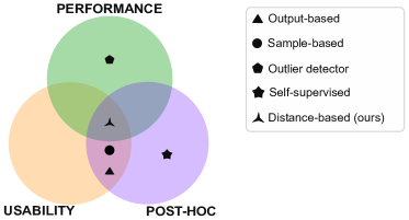
In Figure 1, we illustrate how existing paradigms perform in terms of different desiderata. We are interested in approaches that can be directly used with any model, and so we restrict our analysis to the methods outlined in Table 1.

Method Type Parameters Mod. Level Inf. time Max. Softmax O t 0 ++ Temp. Scaling O t,T 1 ++ KL O t, $p(\theta )$ 2 + Energy Scoring O t,T 1 ++ MC Dropout S t, p 3 - TTA S t, $I_{Aug}$ 2 - - Ours D t, $\mu ,\sigma$ 2 +

Table 1: Comparison between Output- (O), Sample- (S) and Distance-based (D) methods. We compare important factors for applicability: parameters, number of modifications (0-3) and additional inference time from high [- -] to none [++].

Fig. 2: Proposed method for OOD detection on a full-resolution nnU-Net model.

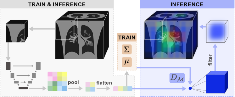
The input image first goes through a series of pre-processing steps and is divided into patches. For each patch, we take the feature maps generated at the end of the encoder during the forward pass. We then project these into a lower-dimensional, flattened subspace. During the training phase, we estimate a Gaussian distribution from the feature space by calculating $\mu$ and $\mathrm{\Sigma }$. At inference time, we calculate the Mahalanobis distance to the training distribution and project the resulting point value into the dimensions of the original patch. Finally, a filtering operation is performed to weigh voxels at the centre more heavily, and the result is aggregated into a volume with the same dimensionality as the input image.

Unlike previous work, our method observes model activations at the end of the encoder. We project these to a lower-dimensional feature space and estimate a multi-variate Gaussian with the training data. During inference, we detect samples with a high Mahalanobis distance to this distribution, which is suitable for quantifying differences in the latent space [34, 8].

3 Material and methods

Our proposed method, visualised in Figure 2, assesses the uncertainty as the distance of new samples to the training distribution in the feature space. First, we extract feature maps from the trained model and project these to a low-dimensional space to ensure a computationally inexpensive calculation. We then estimate a multi-variate Gaussian distribution from ID train samples. At test time, we repeat the feature-extraction process and calculate the Mahalanobis distance.

We first briefly introduce the patch-based nnU-Net architecture in Section 3.1 and outline how our method links to it. In Section 3.2 we describe our proposed method for OOD detection, which follows a three-step process: (1) estimation of a Gaussian distribution from training features (2) extraction of uncertainty masks for test images and finally (3) calculation of subject-level uncertainty scores.

3.1 Patch-based nnU-Net

The nnU-Net is a standardised framework for medical image segmentation [24] that has reported state-of-the-art results across several benchmarks and challenges [18]. Without deviating from the traditional U-Net structure [50], it automatically chooses the best architecture and learning configuration for the training data. The framework also performs pre- and post-processing steps during both training and inference, such as adapting voxel spacing and normalising the intensities.

We use the patch-based full-resolution variant, which is recommended for most applications [24]. After performing all necessary prepossessing operations, input image $x$ is divided into patches following a sliding window approach with an overlap of 50%. This results in $N$ patches ${\left\{x_i\right\}}_{i=1}^N$. A forward pass is made for each patch, at which point we extract feature maps for our method. Predictions for each patch are multiplied by a filtering operation that weights centre-voxels more heavily. Finally, weighted predictions are aggregated into an output mask with dimensionality of the original image.

We also experiment with a 3D HighResNet model [36], which we integrate into the nnU-Net framework and thus follow the same steps for image preparation and combination of the outputs into a coherent prediction.

3.2 Distance-based OOD detection

We are interested in capturing epistemic uncertainty, which arises from a lack of knowledge about the data-generating process. While most uncertainty estimation methods quantify this uncertainty for prediction boundaries, we want to do so for whole regions, which is challenging for OOD data [28].

One way to directly assess epistemic uncertainty is to calculate the distance between training and testing activations. As a model is unlikely to produce reasonable outputs for features far from any seen during training, this is a reliable signal for bad model performance [34].

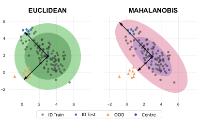
Model activations have covariance, and they do not necessarily resemble the mode for high-dimensional spaces [56], so the Euclidean distance is not appropriate for identifying unusual activation patterns. Instead, inspired by the work of Lee et al. [34], we make use of the Mahalanobis distance $D_{ℳ}$, which rescales samples into a space without covariance. Figure 3 illustrates how the Mahalanobis distance better captures the behaviour of in-distribution data and correctly identifies samples outside the unit circle as OOD.

Fig. 3: Comparison between Euclidean and Mahalanobis distances in a two-dimensional space. Left: Euclidean distance fails to detect that OOD samples (orange triangles) strongly deviate from the expected behaviour of training samples (grey circles). Right: Mahalanobis distance adequately detects OOD samples, assigning them a distance outside the unit circle whilst properly admitting ID test samples (blue circles).

The following sections describe how we leverage the Mahalanobis distance in our approach. Note that only one forward pass is necessary for each patch, keeping the computational overhead at a minimum.

3.2.1 Estimation of the training distribution

We start by estimating a multivariate Gaussian distribution $𝒩(\mu ,\mathrm{\Sigma })$ over training features. For all training patches ${\left\{x_i\right\}}_{i=1}^N$, features $ℱ(x_i)=z_i$ are extracted from the encoder $ℱ$.

For modern segmentation networks, the dimensionality of the extracted features $z_i$ is too large to calculate the covariance $\mathrm{\Sigma }$ in an acceptable time frame. We thus project the latent space into a lower subspace by applying average Pooling operations with a kernel size of $(2,2,2)$ and stride $(2,2,2)$ until the dimensionality falls below $1e4$ elements. Finally, we flatten this subspace and estimate the empirical mean $\mu$ and covariance $\mathrm{\Sigma }$.

$$\mu =\frac{1}{N}\sum _{i=1}^N\widehat{z_i},\mathrm{\Sigma }=\frac{1}{N}\sum _{i=1}^N(\widehat{z_i}-\mu ){(\widehat{z_i}-\mu )}^T$$ (1)

In Table 2 we demonstrate that for a dimensionality of $1e4$ elements we can estimate the covariance in a maximum of a few minutes (rows 3 and 4) with the Scikit Learn on an AMD Ryzen 9 3900X CPU, whereas for higher dimensions the times increase abruptly (row 5).

Nr. samples Dimensionality $\mathrm{\Sigma }$ time (s) $D_{ℳ}$ time (s) 1e3 1e3 0.260 0.001 1e6 1e3 8.480 0.001 1e3 1e4 69.11 0.050 1e4 1e4 81.80 0.051 1e3 2e4 6555.13 0.194 .

Table 2: Times in seconds required for estimating the covariance $\mathrm{\Sigma }$ (column 3) and calculating the Mahalanobis distance $D_{ℳ}$ to one sample (column 4)

3.2.2 Extraction of uncertainty masks

During inference, we estimate an uncertainty mask for a subject following the process illustrated in Figure 2 (right). First, we perform the same preprocessing steps as during training and divide the image into patches. Next, we extract features maps for each patch $x_i$ and project them onto $\widehat{z_i}$ as done during training. We then calculate the Mahalanobis distance (Eq. 2) to the Gaussian distribution estimated in the previous step.

$$D_{ℳ}(\widehat{z_i};\mu ,\mathrm{\Sigma })={(\widehat{z_i}-\mu )}^T{\mathrm{\Sigma }}^{-1}(\widehat{z_i}-\mu )$$ (2)

Each distance is a point estimate for the corresponding patch. We replicate this value to the size of the patch and combine the distances for all patches in the same manner as the segmentation pipeline combines patch outputs into a coherent prediction.

Following the example of the patch-based nnU-Net, we start by initialising a zero-filled tensor with the dimensionality of the original image. We then apply a filtering operation to each patch to weigh voxels at the centre more heavily and add them to the image-level mask.

3.2.3 Subject-level uncertainty

The previous step produces an uncertainty mask with the dimensionality of the input CT scan. In order to effectively identify highly uncertain images, we average over all voxels to obtain one value $𝒰$, and normalise uncertainties between the minimum and doubled maximum uncertainties for ID train data to ensure $𝒰\in [0,1]$.

4 Experimental setup

We start by describing the data used in our experiments in Section 4.1. Afterwards, we state relevant details on our models (Section 4.2). We then introduce all baselines (Section 4.3) and define our evaluation metrics (Section 4.4).

4.1 Data

We train our first model with data from the COVID-19 Lung CT Lesion Segmentation Challenge [51, 1, 9], which we refer to as Challenge or in-distribution (ID). The dataset contains chest CT scans for patients with a confirmed SARS-CoV-2 infection from various centres and countries. The data is also heterogeneous in terms of age, gender, and disease severity of the patients. We use the 199 cases that are made available for the challenge, which we divide into 160 training and 39 testing cases with the nnU-Net random splitting function.

We include results for four types of out-of-distribution samples: (1) dataset shift, where we evaluate the model on two other datasets with differences in the acquisition and population patterns (2) transformation shift where we apply artificial transformations to our ID data, (3) diagnostic shift, where we compare Covid-19 to non-Covid pneumonia patients, and (4) far-OOD, where we use the Spleen and Colon tasks of the Medical Segmentation Decathlon (MSD) [52, 2].

In addition, we perform a study on hippocampus and prostate segmentation from MR images. We train each nnU-Net model with the corresponding task of the MSD and use two and three OOD datasets for hippocampus and prostate, respectively.

4.1.1 Dataset shift

We use two publicly available datasets: Mosmed [44] contains fifty cases and the Radiopedia dataset [25], a further twenty. Both encompass patients with and without confirmed infections. Table 3 provides a summary of data characteristics.

Dataset name Nr. cases Mean image size Mean spacing Challenge 199 [512, 512, 69] [0.8, 0.8, 4.8] Mosmed 50 [512, 512, 41] [0.7, 0.7, 8.0] Radiopedia 20 [560, 571, 176] [1.0, 1.0, 1.0]

Table 3: Characteristics of the Covid-19 lung lesion segmentation datasets.

4.1.2 Transformation shift

We transform the 39 in-distribution test cases with multiple operations from the TorchIO [47] library.

Shift Operation Weak Medium Strong Artefact Ghost intensity (0, 0.2) (0, 0.4) (0, 0.7) Spike intensity (0, 0.2) (0, 0.5) (0, 0.7) Blur STD (0, 0.3) (0, 0.3) (0, 0.3) Noise STD (0, 15) (0, 30) (0, 30) Affine Scales (0.9, 1.4) (0.7, 1.8) (0.6, 2) Rotation degrees 5 8 9 Translation range (-15, 15) (-20, 20) (-20, 20) Isotropic True True False

Table 4: Parameters used to randomly generate artefacts and affine transformations with the TorchIO library. For each type of shift, three transformed datasets are generated with increasingly stronger transformations.

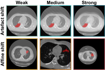
The artefact transformations include ghosting, k-space spikes, Gaussian blurring, and Gaussian noise. Affine transformations include scaling, rotation, and translation. All affine operations can be either isotropic or anisotropic. We deploy the same transformation parameters for the sagittal, coronal, and axial dimensions for the isotropic case. For the anisotropic case, these parameters change for every dimension, causing a stronger shift. For both groups of transformations, we generate three sets (weak, medium, and strong), each with increasingly stronger augmentation parameters. The parameters used are reported in Table 4. Examples of the performed transformations are visualised in Figure 4.

Fig. 4: Top row: Exemplary CT slice with overlaid segmentation mask in red after being transformed to contain artefacts in three magnitudes. Bottom row: Three exemplary CT slices with overlaid segmentation masks after applying affine transformations in three magnitudes. The border colours map each example to their corresponding datasets in Figure 5.

4.1.3 Diagnostic shift

We utilise an in-house dataset of one hundred cases. Fifty patients have pulmonary infection of Covid-19 confirmed by RT PCR test and visible pulmonary Covid-19 lesions in all cases (3/2020 to 12/2020). The remaining fifty cases were composed of various Covid-mimics, manifesting similar pulmonary lesions but acquired prior to the Covid outbreak or tested negative for Covid-19 by RT PCR (3/2017 to 2/2020). Cases were collected and annotated in the RACOON project [49]. Covid-mimics included are viral non-Covid pneumonia, bacterial pneumonia, fungal pneumonia, tuberculosis, chronic obstructive pulmonary disease, cystic fibrosis, interstitial pulmonary fibrosis, acute interstitial pneumonia, cryptogenic organising pneumonia, medication associated pulmonary toxicity, radiogenic pulmonary fibrosis, acute lung embolism, chronic lung embolism, pleural pathologies, pulmonary vasculitis, bronchial carcinoma, pulmonary metastasis, as well as a control case without any lung pathologies.

A clinical radiologist with 8 years of experience in reading chest CT reviewed all scans and found them to be of good enough quality for accurate visual diagnosis. Manual annotations of the entire image stack were performed slice-by-slice by two independent readers trained in the delineation of GGOs and pulmonary consolidations. Central vascular structures and central bronchial structures were excluded from all annotations. Care was taken to differentiate between artefacts and GGO. Consolidations were defined as visible in a soft tissue window and at least 5 mm in size. An expert radiologist reader reviewed all delineations. In Table 5 we report some details on the demographic distribution.

Age Gender Voltage mAs Covid-19 57.17 [49/67] 16% 100 121.21 $\pm$ 55.91 Non-Covid 60.24 [47/73] 42% 120 114.77 $\pm$ 82.56

Table 5: In-house data cohort with 50 Covid-19 and 50 non-Covid cases. We report the age (median Q1/Q3), gender (f/m), voltage (median kV), and tube current-time product (mAs).

4.1.4 MRI tasks

For hippocampus we consider three T1-weighted datasets: the MSD task, which we denote MSD H, and contains healthy and schizophrenia patients, the Dryad [31] dataset with fifty healthy subjects and the Harmonized Hippocampal Protocol data [7] (HarP) with senior subjects, some of which have Alzheimer’s.

For the segmentation of the prostate in T2-weighted MRIs we use a corpus of four datasets including the MSD data (MSD P) and three OOD sets: the cases provided in the NCI-ISBI 2013 Challenge [5] (ISBI) and the I2CVB [35] and UCL [38] datasets as made available by Liu et al. [39]. To align label characteristics, we unify the labels of head and body for the hippocampus and of central gland and peripheral area for the prostate. A summary of the relevant dataset characteristics can be found in Table 6.

Dataset name Nr. cases Mean image size Mean spacing MSD H 260 [50, 35, 36] [1.0, 1.0, 1.0] Dryad 50 [64, 64, 48] [1.0, 1.0, 1.0] HarP 270 [64, 64, 48] [1.0, 1.0, 1.0] MSD P 32 [316, 316, 19] [1.0, 1.0, 1.0] ISBI 30 [384, 384, 19] [0.5, 0.5, 3.7] UCL 13 [384, 384, 24] [0.5, 0.5, 3.3] I2CVB 19 [384, 384, 64] [0.5, 0.4, 1.3]

Table 6: Characteristics of the MR hippocampus (top) and prostate (bottom) segmentation datasets. Models were trained with the respective tasks of the Medical Segmentation Decathlon.

4.2 Models

We train three patch-based nnU-Nets [24] and one HighResNet [36] on a Tesla T4 GPU. Our configurations have patch sizes of $[256,256,28]$, $[56,40,40]$ and $[320,320,20]$ for the Challenge, MSD H and MSD P tasks, respectively. In all cases, adjacent patches overlap by 50%, and we train with a loss of Dice (smoothing 1e-5) and Binary Cross-entropy weighted equally until after convergence. Training begins with a learning rate of 0.01 and a weight decay of 3e-5. No test-time augmentation was applied to extract predictions, as this signifies a speed-up of 8 times for 3D data.

4.3 Baselines

We compare our approach to output- and sample-based techniques that assess uncertainty information by performing inference on a trained model. Max. Softmax consists of taking the maximum softmax output [19]. Temp. Scaling performs temperature scaling on the outputs before applying the softmax operation [16]. KL from Uniform computes the KL divergence from a uniform distribution [21]. Note that all three methods output a confidence score (higher is more certain), which we invert to obtain an uncertainty estimate (lower is more certain). Energy Scoring [40] assesses uncertainty as the logarithmic sum of the softmax denominator.

MC Dropout [12] consists of doing several forward passes whilst activating the Dropout layers that would usually be dormant during inference. We perform $10$ forward passes. Test-Time Augmentation (TTA) follows a similar strategy by augmenting images during testing [55]. We use image-flip as augmentation and generate eight predictions by flipping the input image once clockwise and counter-clockwise for every axis. We report the standard deviation between outputs as an uncertainty score for both methods.

For all baselines and our proposed method we calculate a subject-level metric by averaging voxel values, and normalise the uncertainty range between the minimum and doubled maximum uncertainty represented in ID train data. For Energy Scoring and Temp. Scaling, we always report the result with lowest ESCE from among three different temperature settings $T\in \{1,10,100\}$.

4.4 Metrics

For OOD detection, we calculate the 95% true positive rate (TPR) boundary on ID data, i.e. the boundary that covers at least 95% of train samples. Samples with uncertainties greater than this boundary are predicted to be OOD. We report the false positive rate, defined as

$$FPR=\frac{FP}{FP+TN},$$ (3)

where a false positive (FP) is an OOD sample incorrectly deemed to be in-distribution, the Detection Error

$$Error=\frac{1}{2}(1-TPR)+\frac{1}{2}FPR$$ (4)

and the area under the receiving operating curve (AUC), calculated with the Scikit Learn library [46].

While the detection of OOD samples is a first step in assessing the suitability of a model for a new image, an ideal uncertainty metric would inversely correlate with model performance. For this, we calculate the Expected Segmentation Calibration Error (ESCE). Inspired by Guo et al. [16], we divide the $n$ test scans into $M=10$ interval bins $B_m$. For each bin, the absolute difference is calculated between average Dice $(Dice(B_m))$ and inverse average uncertainty $(1-𝒰(B_m))$ for samples in the bin. A weighted average is reported that weights the score for each bin by the number of samples in it (Eq. 5).

$$ESCE=\sum _{m=1}^M\frac{\left|B_m\right|}{n}\left|Dice(B_m)-(1-𝒰(B_m))\right|$$ (5)

5 Results

Fig. 5: Performance deterioration of a model trained with ID (Challenge) data and tested on (1) Radiopedia and Mosmed; Challenge test cases after applying (2) artefact and (3) affine transformations with different levels of intensity; and (4) in-house Covid-19 and non-Covid pneumonia patients.

We first analyse the dataset shift scenario, where a model trained on the Challenge dataset is tested on publicly available Radiopedia and Mosmed cases (Section 5.1). Afterwards, we evaluate how robust the model is against the presence of artefacts and affine transformations of different magnitudes and explore to what extent these are correctly detected (Section 5.2). As a third setting, we apply our method to an in-house data cohort with both Covid-19 and non-Covid patients in Section 5.3.

In Section 5.4, we perform a far-OOD study where we examine whether our method detects samples very far from the raining distribution. We then carry out an ablation study where we measure the use of different network layers for feature extraction (Section 5.5) and repeat the dataset shift experiments on a HighResNet model (Section 5.6). In all these experiments, we explore whether our method can distinguish between ID cases – test subjects from the Challenge data – and OOD images. We qualitatively look into exemplary predictions and corresponding uncertainty scores in Section 5.7.

Finally, in Section 5.8, we evaluate the transferability of our method to MR data, where we look at hippocampus and prostate segmentation tasks.

5.1 Dataset shift

In Table 7, we report the performance of our proposed method and six other approaches in identifying the OOD samples, i.e. samples from the Mosmed or Radiopedia datasets for which the model produces unreliable predictions (see Figure 5). Following previous research in OOD detection [37], we find the uncertainty boundary that covers 95% of in-distribution train samples and deem cases with uncertainties beyond the ID 95th percentile threshold as OOD. Our distance-based method is the only approach that successfully flags cases far from the training distribution, as shown by a low detection error and FPR and an AUC close to one.

Method ESCE $\downarrow$ Error $\downarrow$ FPR $\downarrow$ AUC $\uparrow$ Max. Softmax .39 .43 .84 .61 MC Dropout .28 .41 .79 .75 KL .38 .44 .83 .69 TTA .36 .41 .77 .74 Temp. Scaling .02 .47 .89 .42 Energy Scoring .46 .51 .90 .31 Ours .15 .09 .04 .96

Table 7: Dataset shift results. Ability of assessing segmentation quality as Estimated Segmentation Calibration Error (ESCE) and identifying samples from Radiopedia and Mosmed as OOD in terms of Detection Error (Error), False Positive Rate (FPR) and Area Under the ROC (AUC).

We plot the Dice score against normalised uncertainty for the three best-performing methods in Figure 6. The vertical line marks the 95% TPR boundary. We consider predictions with a Dice score lower than 0.6 to be of low quality as they diverge significantly from the ground truth [54] and, for the task of Covid-19 lesion segmentation, provide a misleading assessment of the spread of the infection.

Fig. 6: Dice coefficient against normalised uncertainty for test ID (black circles) and OOD (orange triangles) scans. The ID samples are from the Challenge dataset, and the OOD ones from Mosmed or Radiopedia. The grey vertical line marks the 95% TPR for ID train data. Samples to the right are predicted to be OOD. Clinically relevant is the lower left (red) quadrant that houses silent failures, i.e. predictions with a Dice 0.6 and low uncertainty scores.

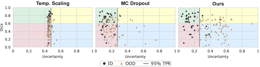
The lower left (red) quadrant is critical for the safe use of segmentation models, as it houses silent failures for which low-quality predictions are made but which are not identified as such. Only our method assigns sufficiently large uncertainty estimates to poorly segmented OOD samples, excluding them from this section. Nevertheless, the upper right (yellow) quadrant shows that our method is too conservative in estimating uncertainties, not identifying samples for which the model produces good segmentations. This overly cautious behaviour potentially leads to an under-utilisation of the model for cases that are technically OOD but have very apparent lesions which are easy to segment; though any amount of safe utilisation is advantageous. Another limitation of the proposed method is that it fails to identify ID samples that the model segments incorrectly due to the lesions being too small or different from those seen in the training data, highlighting the fact that OOD detection is only part of a thorough QA process.

Regarding the estimation of segmentation quality, Temp. Scaling reaches the lowest ESCE (first column in Table 7), but a closer inspection of Figure 6 (left) displays that this is due to most uncertainties clustering on the fifth bin. An ideal segmentation calibration would house all samples in the upper left (green) and lower right (blue) quadrants.

5.2 Artefact and affine shifts

The dataset shift scenario observed in the previous section depicts a realistic setting whether there are several potential degrees of variation between the training data and cases encountered during deployment. However, it is difficult to assess whether the model performance falls due to (a) changes in the acquisition process, (b) another patient population or simply (c) a different delineation process for ground truth segmentation masks. Subsequently, we cannot confidently assess why cases are flagged as OOD. We therefore artificially transform the same ID test cases in two different ways and three levels of magnitude. More than any other explored scenario, these images could be deemed near-OOD [10]. Nevertheless, there is a significant performance deterioration for transformed images, which grows with the magnitude of the perturbation (Figure 5).

We start by simulating the presence of common image artefacts. In Figure 7, we visualise the results of our method.

Fig. 7: Dice coefficient against normalised uncertainty. Black circles are the test ID (unmodified Challenge) images, and the remaining markers stand for the same Challenge images after applying transformations to simulate common artefacts.

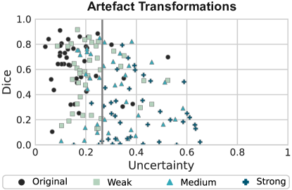
While non-transformed (original) cases are correctly assigned low uncertainty scores and most heavily transformed samples are identified as OOD, several samples for which bad segmentations are produced are not identified. Most of these are only weakly transformed (mint-coloured squares). On the other hand, many weakly transformed cases for which good segmentations are produced are correctly assigned low uncertainties despite not being ID. Most heavily transformed images (turquoise crosses) are correctly deemed too far from the training distribution to have reliable predictions.

Fig. 8: Distribution of uncertainty scores estimated by our proposed method for the artefact shift and affine shift scenarios. In general, the uncertainties increase with the intensity of the transformations.

A similar situation occurs when we apply affine transformations to simulate geometric changes (Figure 9). These could arise from shifting population patterns, scans being acquired for different ranges, or using other acquisition parameters. Our method deems many weakly transformed cases (yellow squares) to be ID. This is positive as good segmentations are available for most cases. However, a few failure cases are not adequately identified.

Fig. 9: Dice coefficient against normalised uncertainty. Black circles are the test ID (unmodified Challenge) images, and the remaining markers stand for the same Challenge images after applying transformations to simulate affine shifts.

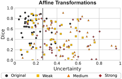
Table 8 compares several approaches in terms of OOD detection and segmentation quality assessment. While our method displays an acceptable calibration error and the best OOD detection performance, this near-OOD problem proves more difficult than dataset shift. It particularly seems to be very difficult to reliably detect image artefacts.

Method ESCE $\downarrow$ Error $\downarrow$ FPR $\downarrow$ AUC $\uparrow$ Max. Softmax .46/.44 .48/.46 .94/.89 .55/.56 MC Dropout .44/.44 .51/.51 1.0/.99 .22/.23 KL .46/.44 .48/.46 .91/.86 .58/.57 TTA .43/.41 .46/.38 .87/.72 .63/.61 Temp. Scaling .05/.04 .51/.35 .95/.62 .50/.76 Energy Scoring .52/.51 .53/.33 .92/.53 .49/.76 Ours .26/.21 .29/.18 .45/.24 .83/.89

Table 8: Transformation shift results. Segmentation calibration (as ESCE) and OOD detection scores between original Challenge images and cases modified with synthetic artefacts and affine transformations, respectively.

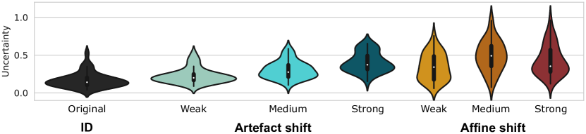
We further visualise the uncertainty ranges assigned to each shift and magnitude in Figure 8. As expected, the uncertainty increases with the degree of transformation for artefact shifts. For affine shifts, medium changes result in similar uncertainties to strong ones. This is likely due to the selected transformation sequences being too similar (see Table 4), which results in a similar performance for medium and strong artefacts (Figure 5).

In general, we can conclude that the uncertainty correlates positively with the degree of deformation and inversely with model performance. Affine transformations also have a more pronounced effect on the uncertainties (Figure 8). This possibly stems from the training data containing similar patterns to those introduced by the weaker artefact transformations.

5.3 Diagnostic shift

We have not yet analysed how the segmentation model performs across disease patterns. To explore this, we segment lung lesions in the form of GGOs and consolidations for an in-house cohort of 50 Covid-19 and 50 non-Covid cases. The performance of the model on the non-Covid cases is significantly worse. Table 9 summarises our findings, and we plot our uncertainty assessment in Figure 10.

Method ESCE $\downarrow$ Error $\downarrow$ FPR $\downarrow$ AUC $\uparrow$ Max. Softmax .29/.42 .22/.32 .42/.62 .86/.87 MC Dropout .22/.38 .30/.46 .58/.90 .84/.69 KL .29/.42 .23/.33 .40/.60 .88/.89 TTA .25/.32 .19/.17 .32/.28 .89/.95 Temp. Scaling .07/.05 .34/.54 .62/1.0 .78/.06 Energy Scoring .38/.54 .49/.56 .86/1.0 .61/.05 Ours .16/.26 .13/.15 .14/.18 .93/.92

Table 9: Diagnostic shift results. Segmentation calibration (as ESCE) and OOD detection scores between test ID Challenge images and in-house cases with and without Covid-19, respectively.

Our method reliably detects cases from our in-house cohort, though it does not distinguish between Covid-19 and non-Covid cases. Though ideally Covid-19 cases for which good predictions are produced should be deemed low-uncertainty, the fact that badly segmented non-Covid cases are flagged as OOD is more relevant for clinical use as unsure good predictions are preferred over confident faulty ones.

Fig. 10: Dice coefficient against normalised uncertainty for ID test (Challenge)

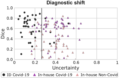
data and in-house chest CTs of Covid-19-positive (purple triangles) and non-Covid (pink triangles) patients.

5.4 Far-OOD examinations

We have extensively examined near-OOD [10] cases where a performance deterioration is unexpected. In contrast, far-OOD situations occur when an input is erroneously fed into a model, and there is no realistic expectation that a model can produce a sensible prediction.

In Table 10, we examine what happens when we feed CT spleen and colon cancer examinations from the Medical Segmentation Decathlon into our model trained to segment pulmonary lesions from chest CTs. Our method distinguishes between ID and far-OOD cases, correctly identifying all colon examinations as OOD (FPR = 0) and showing detection errors of up to 0.1 for both anatomies.

Method ESCE $\downarrow$ Error $\downarrow$ FPR $\downarrow$ AUC $\uparrow$ Max. Softmax .58/.71 .44/.42 .85/.81 .89/.89 MC Dropout .50/.64 .37/.36 .68/.66 .88/.87 KL .59/.72 .44/.42 .85/.81 .88/.88 TTA .48/.58 .18/.22 .29/.37 .95/.95 Temp. Scaling .62/.71 .48/.42 .93/.81 .79/.89 Energy Scoring .31/.16 .49/.51 .93/1.0 .50/.50 Ours .34/.41 .10/.06 .07/.00 .96/.98

Table 10: Far-OOD results. Segmentation calibration (as ESCE) and OOD detection scores between test ID Challenge images and CT scans for spleen and colon examinations, respectively.

5.5 Ablation study

We evaluate which features are most expressive for detecting distribution shifts in Table 11. We compare the use of activations at the middle of the network, more specifically the convolutional (Conv) parameters of the sixth encoding block (EB) against those of the first decoding block (DB), and features at the beginning (1st EB) and final end (6th DB) of the architecture. In addition, we look into the use of batch normalisation (BN) layers, as these normalise layer inputs and therefore contain domain information [23]. The results show that features at the middle of the network (6th EB Conv, followed by 6th EB BN and 1st DB Conv) are the most suitable for detecting distribution shifts.

Features ESCE $\downarrow$ Error $\downarrow$ FPR $\downarrow$ AUC $\uparrow$ 6th EB Conv .15/.23 .09/.24 .04/.35 .96/.86 6th EB BN .18/.23 .11/.25 .09/.37 .95/.85 1st EB Conv .42/.24 .56/.70 .13/.40 .81/.21 1st EB BN .52/.45 .50/.50 .00/.00 .51/.51 1st DB Conv .17/.25 .09/.25 .06/.38 .96/.84 6th DB Conv .52/.45 .50/.50 .00/.00 .50/.50

Table 11: Ablation study on the usability of feature maps. OOD detection and segmentation calibration for our proposed method using different convolutional (Conv) and batch normalisation (BN) at different encoding (EB) and decoding blocks (DB). The results are for the dataset shift and transformed (including both artefact and affine shifts) scenarios, respectively.

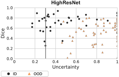
5.6 HighResNet model

Not all segmentation models follow an encoder-decoder structure. For instance, the HighResNet [36] uses dilated convolutions and residual blocks to produce accurate segmentations. That raises the questions of whether our proposed approach would be effective on this architecture and which features would be most helpful for detecting distribution shifts. We report these results for the dataset shift scenario in Table 12. The upper section summarises the results for all baselines, and the lower part shows the performance of our proposed method for three different feature maps.

Method ESCE $\downarrow$ Error $\downarrow$ FPR $\downarrow$ AUC $\uparrow$ Max. Softmax .35 .48 .94 .57 MC Dropout .35 .49 .96 .59 KL .34 .46 .90 .60 TTA .35 .48 .90 .61 Temp. Scaling .35 .48 .93 .54 Energy Scoring .58 .49 .97 .50 7th Conv Block .41 .47 .00 .94 6th Dil Conv Block .58 .50 .00 .50 12th Dil Conv Block .33 .37 .00 .84

Table 12: HighResNet results. Segmentation calibration (as ESCE) and OOD detection scores between test ID Challenge images and OOD samples belonging to the Radiopedia or Mosmed datasets, for a HighResNet model trained on Challenge. The bottom part of the table shows three variations of our method with different feature maps: the 7th conv. block, the 6th block with dilated conv., and the 12th (last) block with dilated convolutions.

The HighResNet architecture is divided into four sections: (1) seven convolutional blocks, (2) six blocks with dilated convolutions using a dilation factor of 2, (3) six dilated convolutional blocks with a factor of 4, and (4) a final convolutional block. Residual connections with identity mapping are also included every two blocks to join features at different levels. We test the use of three feature maps: the last (7th) convolutional block, the last (6th) dilated convolutional block with factor 2, and the last (12th) dilated convolutional block.

The best results are for the variant of our method which uses the last block with dilated convolutions. Though the FPR and AUC are encouraging, the detection error is relatively high, suggesting that the TPR is low as the 95% TPR on ID train data does not cover a significant portion of ID test samples (see Eq. 4). We plot the performance of the network vs. normalised uncertainties for the best-performing features in Figure 11. A separation is noticeable between ID (Challenge) and OOD (Radiopedia and Mosmed), but the uncertainty boundary – as hypothesised from the high Detection Error – is too low. This means that OOD samples are correctly detected, yet the model is under-utilised.

Fig. 11: Dice coefficient against normalised uncertainty for the variant using the 12th Dil. Conv. Block. Black circles are test ID (Challenge) images, and orange triangles are OOD cases from Radiopedia or Mosmed.

5.7 Qualitative evaluation

Fig. 12: Axial and coronal slices with overlaid predictions and ground truths and volume renderings of the predictions for three different subjects. First column: a good prediction. Second column: a poor prediction for an OOD case which our method successfully detects. Though there are considerable differences to the ground truth, these errors are not directly noticeable even for trained observers. Third column: a good prediction for an OOD case.

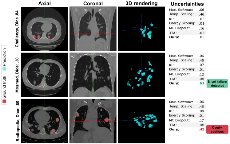
We now take a detailed view of some cases in Figure 12. The first column shows an in-distribution Challenge case with a good prediction. The second and third cases are from Mosmed and Radiopedia, respectively. While the Mosmed prediction is significantly different from the ground truth (incorrectly marking several regions as lesions), a good segmentation is produced for the third case.

We first notice the complexity of assessing whether a segmentation mask for lung lesions is correct. An untrained observer would not be able to detect that the second segmentation is so different from the ground truth, and even trained radiologists may not directly identify this error, as GGOs can manifest in superior lobes and with multiple connected components [45]. Similarly, all methods fail to detect this case except for our distance-based method, which assigns an uncertainty of 0.61.

The prediction for the third case over-segments some lesions, though if we observe the difference between the Challenge and Radiopedia ground truth masks, we notice that delineations are courser for the first case (we see in the first image that broad regions around lesions are marked as infected). Therefore, the model learns to mimic this behaviour. Beyond this, the segmentation model correctly detects all lesions and only creates a very small additional component. Here, our method makes an overly cautious uncertainty assessment, assigning this case an uncertainty of .43 which falls beyond the 95% TPR boundary.

5.8 Application to MRI data

Magnetic Resonance Imaging (MRI) data is even more susceptible to changes in the acquisition conditions than CTs, as there is no consensus on the calibration of intensity values. This causes the performance of segmentation models trained on MR tasks to deteriorate on OOD data [57, 30].

In this section, we evaluate how our proposed method can help detect such distribution shifts on nnU-Net models trained with the hippocampus and prostate tasks of the MSD. Figure 13 illustrates that while the initial performance of the models is over 0.8 Dice on in-distribution test data (MSD H and MSD P), it falls significantly for the OOD datasets.

Fig. 13: Performance as Dice score of models trained with MSD H (left) and MSD P (right) data for hippocampus and prostate segmentation, respectively. Plotted are the ID test (in dark blue) and OOD scores.

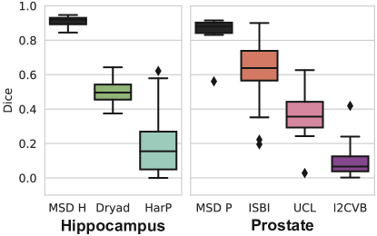
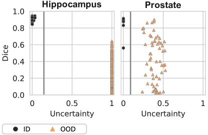
Table 13 summarises our results on OOD detection, and we visualise the uncertainties of our method in Figure 14. We immediately see that – for both MR segmentation tasks – detecting OOD cases is much easier than for chest CT. In all cases, the proposed method correctly distinguishes ID from OOD data. This is likely due to the inherent variability across MRI datasets in terms of intensity histogram and fields-of-view. The last row includes a far-OOD case where we look to detect MSD H cases on the model trained with MSD P and vice versa. This also seems to be an easy problem, and our method correctly identifies all OOD cases.

Method ESCE $\downarrow$ Error $\downarrow$ FPR $\downarrow$ AUC $\uparrow$ Max. Softmax .20/.36 .05/.49 .00/.82 1.0/.74 MC Dropout $N=10$ .53/.08 .50/.01 1.0/.02 .40/1.0 MC Dropout $N=100$ .48/.14 .53/.00 1.0/.00 .12/1.0 KL .18/.15 .05/.16 .00/.16 1.0/.83 TTA .20/.40 .09/.25 .00/0.0 1.0/.83 Temp. Scaling .12/.36 .03/.49 .00/.82 1.0/.74 Energy Scoring .68/.53 .50/.49 1.0/.98 .50/.12 Ours .21/.19 .00/.00 .00/.00 1.0/1.0 Ours far-OOD .08/.01 .00/.00 .00/.00 1.0/1.0

Table 13: MRI results. Segmentation calibration (as ESCE) and OOD detection scores between test ID and OOD cases for hippocampus and prostate, respectively. The networks were trained with MSD H and MSD P data, respectively, so these cases are ID. The last row summarises the results for the far-OOD case of detecting MSD P cases on the MSD H model and vice versa.

Fig. 14: Dice coefficient against normalised uncertainty for the segmentation of the hippocampus (left) and prostate (right) in MR images. Black circles are test ID (MSD) images, and orange triangles are OOD cases.

6 Discussion

Uncertainty quantification is an unavoidable cornerstone for safely deploying predictive models in real clinics. Our results show that the proposed distance-based approach provides valuable information for detecting images that the model is unprepared to segment.

As distance-based OOD detection can seamlessly augment any segmentation pipeline, there is no reason against performing this quality check. However, we found in our analysis several areas where there is room for improvement. Almost all our experiments showed that our method is overly cautious in its uncertainty estimation. Specifically, many OOD cases for which the model did produce adequate segmentation were deemed highly uncertain. Only for the artefact shift scenario were weekly transformed samples segmented.

The artefact and affine shifts experiments show that – for both explored synthetic scenarios – the produced distances grow linearly with the degree of change and are inversely proportional to segmentation quality. This is ideal behaviour for an uncertainty metric. However, the same does not hold for the dataset shift and diagnostic shift settings. Particularly for the last scenario, our method assigns similar uncertainties to both Covid-19 and non-Covid cases, even though segmentations are much worse for the last group. Further research should explore which distribution shifts negatively affect model performance, and how these can be distinguished from harmless shifts.

This discrepancy might also be associated with the relatively higher variety of the pulmonary patterns for the labels GGO and consolidation present in the various pulmonary diseases making up the non-Covid-19 group, as compared to the Covid-19 group. This group was, however, purposefully designed to resemble a broad range of non-Covid-associated pulmonary disease patterns, which represent Covid-19-mimics. Further, the large time frame in which these cases were collected, as well as a differing distribution amongst the three CT scanners used to generate these cases, might contribute to this finding.

Our experiments also show that our distance-based approach does not adequately detect poorly segmented cases for in-distribution data. This shortcoming reinforces the notion that uncertainty estimation methods, which are mainly designed to detect uncertain predictions in ID data, should complement OOD detection in practice. However, neither MC Dropout nor TTA were successful at assessing segmentation quality.

Our ablation study shows that intermediate network layers are the most informative for assessing distribution shifts. OOD samples do not display patterns that differ sufficiently from training samples in feature maps near the inputs or outputs of the model. In contrast, activations in intermediate layers allow the separation between ID and OOD cases. For the HighResNet model, which does not follow an encoder-decoder structure, dilated convolutions near the end of the model resulted in the best uncertainty estimates.

Finally, our far-OOD experiments on both CT and MR data confirm that our proposed method accurately detects cases very far from the training distribution. Such far-OOD cases may arise when an erroneous input is fed into the model, and automatically signalling such mistakes can be helpful for inexperienced users.

7 Conclusions

Despite ample progress in the development of segmentation solutions, these are not ready to be deployed in clinical practice. The main reason behind this is the fact that predictive models fail silently, coupled with a lack of appropriate quality controls to detect such behaviour. This is particularly true when it is not trivial to identify a faulty output, such as segmentation of SARS-CoV-2 lung lesions.

Increasingly, institutions are taking part in initiatives to gather large amounts of annotated, heterogeneous data and release it to the public. This could allow the training of robust models and potentially alleviate the burden of radiologists. However, even models trained with heterogeneous cohorts are susceptible to distribution shifts.

We propose a distance-based method to detect images far from the training distribution in a low-dimensional feature space, and find that this is a lightweight and flexible way to signal when a model prediction should not be trusted.

Future work should explore how to improve uncertainty calibration by identifying high-quality predictions. For now, our work increases clinicians’ trust while translating trained neural networks from challenge participation to real clinics.

References

- An et al. [2020] An, P., Xu, S., Harmon, S., Turkbey, E., Sanford, T., Amalou, A., Kassin, M., Varble, N., Blain, M., Anderson, V., et al., 2020. Ct images in covid-19. Cancer Imaging Archive .
- Antonelli et al. [2022] Antonelli, M., Reinke, A., Bakas, S., Farahani, K., Kopp-Schneider, A., Landman, B.A., Litjens, G., Menze, B., Ronneberger, O., Summers, R.M., et al., 2022. The medical segmentation decathlon. Nat. Communications 13, 1–13.
- Ashukha et al. [2019] Ashukha, A., Lyzhov, A., Molchanov, D., Vetrov, D., 2019. Pitfalls of in-domain uncertainty estimation and ensembling in deep learning, in: International Conference on Learning Representations.
- Bevandić et al. [2019] Bevandić, P., Krešo, I., Oršić, M., Šegvić, S., 2019. Simultaneous semantic segmentation and outlier detection in presence of domain shift, in: German Conference on Pattern Recognition, Springer. pp. 33–47.
- Bloch et al. [2015] Bloch, N., Madabhushi, A., Huisman, H., Freymann, J., Kirby, J., Grauer, M., Enquobahrie, A., Jaffe, C., Clarke, L., Farahani, K., 2015. NCI-ISBI 2013 challenge: automated segmentation of prostate structures. doi:http://doi.org/10.7937/K9/TCIA.2015.zF0vlOPv.
- Blundell et al. [2015] Blundell, C., Cornebise, J., Kavukcuoglu, K., Wierstra, D., 2015. Weight uncertainty in neural network, in: International Conference on Machine Learning, PMLR. pp. 1613–1622.
- Boccardi et al. [2015] Boccardi, M., Bocchetta, M., Morency, F.C., Collins, D.L., Nishikawa, M., Ganzola, R., Grothe, M.J., Wolf, D., Redolfi, A., Pievani, M., et al., 2015. Training labels for hippocampal segmentation based on the eadc-adni harmonized hippocampal protocol. Alzheimer’s & Dementia 11, 175–183.
- Çallı et al. [2019] Çallı, E., Murphy, K., Sogancioglu, E., van Ginneken, B., 2019. Frodo: Free rejection of out-of-distribution samples: application to chest x-ray analysis, in: International Conference on Medical Imaging with Deep Learning–Extended Abstract Track.
- Clark et al. [2013] Clark, K., Vendt, B., Smith, K., Freymann, J., Kirby, J., Koppel, P., Moore, S., Phillips, S., Maffitt, D., Pringle, M., et al., 2013. The cancer imaging archive (tcia): maintaining and operating a public information repository. J. of Digital Imaging 26, 1045–1057.
- Fort et al. [2021] Fort, S., Ren, J., Lakshminarayanan, B., 2021. Exploring the limits of out-of-distribution detection. Advances in Neural Inf. Processing Systems 34.
- Fuchs et al. [2021] Fuchs, M., Gonzalez, C., Mukhopadhyay, A., 2021. Practical uncertainty quantification for brain tumor segmentation, in: Medical Imaging with Deep Learning.
- Gal and Ghahramani [2016] Gal, Y., Ghahramani, Z., 2016. Dropout as a bayesian approximation: Representing model uncertainty in deep learning, in: International Conference on Machine Learning, PMLR. pp. 1050–1059.
- Golan and El-Yaniv [2018] Golan, I., El-Yaniv, R., 2018. Deep anomaly detection using geometric transformations. Advances in Neural Inf. Processing Systems 31.
- Gonzalez et al. [2021] Gonzalez, C., Gotkowski, K., Bucher, A., Fischbach, R., Kaltenborn, I., Mukhopadhyay, A., 2021. Detecting when pre-trained nnu-net models fail silently for covid-19 lung lesion segmentation, in: International Conference on Medical Image Computing and Computer-Assisted Intervention, Springer. pp. 304–314.
- Gonzalez and Mukhopadhyay [2021] Gonzalez, C., Mukhopadhyay, A., 2021. Self-supervised out-of-distribution detection for cardiac CMR segmentation, in: Proceedings of the Fourth Conference on Medical Imaging with Deep Learning, PMLR. pp. 205–218. URL: https://proceedings.mlr.press/v143/gonzalez21a.html.
- Guo et al. [2017] Guo, C., Pleiss, G., Sun, Y., Weinberger, K.Q., 2017. On calibration of modern neural networks, in: International Conference on Machine Learning, PMLR. pp. 1321–1330.
- Hein et al. [2019] Hein, M., Andriushchenko, M., Bitterwolf, J., 2019. Why relu networks yield high-confidence predictions far away from the training data and how to mitigate the problem, in: Proceedings of the IEEE Conference on Computer Vision and Pattern Recognition, pp. 41–50.
- Henderson [2021] Henderson, E., 2021. Leading pediatric hospital reveals top ai models in covid-19 grand challenge. news-medical.net. Accessed: 2021-02-28.
- Hendrycks and Gimpel [2017] Hendrycks, D., Gimpel, K., 2017. A baseline for detecting misclassified and out-of-distribution examples in neural networks, in: International Conference on Learning Representations.
- Hendrycks et al. [2018] Hendrycks, D., Mazeika, M., Dietterich, T., 2018. Deep anomaly detection with outlier exposure, in: International Conference on Learning Representations.
- Hendrycks et al. [2019] Hendrycks, D., Mazeika, M., Kadavath, S., Song, D., 2019. Using self-supervised learning can improve model robustness and uncertainty. Advances in Neural Inf. Processing Systems 32.
- Hu et al. [2020] Hu, Y., Jacob, J., Parker, G.J., Hawkes, D.J., Hurst, J.R., Stoyanov, D., 2020. The challenges of deploying artificial intelligence models in a rapidly evolving pandemic. Nat. Machine Intelligence 2, 298–300.
- Ioffe and Szegedy [2015] Ioffe, S., Szegedy, C., 2015. Batch normalization: Accelerating deep network training by reducing internal covariate shift, in: International Conference on Machine Learning, PMLR. pp. 448–456.
- Isensee et al. [2021] Isensee, F., Jaeger, P.F., Kohl, S.A., Petersen, J., Maier-Hein, K.H., 2021. nnu-net: a self-configuring method for deep learning-based biomedical image segmentation. Nat. Methods 18, 203–211.
- Jun et al. [2020] Jun, M., Cheng, G., Yixin, W., Xingle, A., Jiantao, G., Ziqi, Y., Minqing, Z., Xin, L., Xueyuan, D., Shucheng, C., Hao, W., Sen, M., Xiaoyu, Y., Ziwei, N., Chen, L., Lu, T., Yuntao, Z., Qiongjie, Z., Guoqiang, D., Jian, H., 2020. Covid-19 ct lung and infection segmentation dataset. URL: https://doi.org/10.5281/zenodo.3757476, doi:10.5281/zenodo.3757476.
- Jungo et al. [2020] Jungo, A., Balsiger, F., Reyes, M., 2020. Analyzing the quality and challenges of uncertainty estimations for brain tumor segmentation. Frontiers in Neuroscience 14, 282.
- Jungo and Reyes [2019] Jungo, A., Reyes, M., 2019. Assessing reliability and challenges of uncertainty estimations for medical image segmentation, in: International Conference on Medical Image Computing and Computer-Assisted Intervention, Springer. pp. 48–56.
- Kendall and Gal [2017] Kendall, A., Gal, Y., 2017. What uncertainties do we need in bayesian deep learning for computer vision? Advances in Neural Inf. Processing Systems 30.
- Kohl et al. [2018] Kohl, S.A., Romera-Paredes, B., Meyer, C., Fauw, J.D., Ledsam, J.R., Maier-Hein, K.H., Eslami, S.A., Rezende, D.J., Ronneberger, O., 2018. A probabilistic u-net for segmentation of ambiguous images, in: Proceedings of the 32nd International Conference on Neural Information Processing Systems, pp. 6965–6975.
- Kondrateva et al. [2021] Kondrateva, E., Pominova, M., Popova, E., Sharaev, M., Bernstein, A., Burnaev, E., 2021. Domain shift in computer vision models for mri data analysis: an overview, in: Thirteenth International Conference on Machine Vision, SPIE. pp. 126–133.
- Kulaga-Yoskovitz et al. [2015] Kulaga-Yoskovitz, J., Bernhardt, B.C., Hong, S.J., Mansi, T., Liang, K.E., Van Der Kouwe, A.J., Smallwood, J., Bernasconi, A., Bernasconi, N., 2015. Multi-contrast submillimetric 3 tesla hippocampal subfield segmentation protocol and dataset. Scientific Data 2, 1–9.
- Lakshminarayanan et al. [2017] Lakshminarayanan, B., Pritzel, A., Blundell, C., 2017. Simple and scalable predictive uncertainty estimation using deep ensembles. Advances in Neural Inf. Processing Systems 30, 6402–6413.
- Lee et al. [2018a] Lee, K., Lee, H., Lee, K., Shin, J., 2018a. Training confidence-calibrated classifiers for detecting out-of-distribution samples, in: International Conference on Learning Representations.
- Lee et al. [2018b] Lee, K., Lee, K., Lee, H., Shin, J., 2018b. A simple unified framework for detecting out-of-distribution samples and adversarial attacks, in: Advances in Neural Information Processing Systems, pp. 7167–7177.
- Lemaître et al. [2015] Lemaître, G., Martí, R., Freixenet, J., Vilanova, J.C., Walker, P.M., Meriaudeau, F., 2015. Computer-aided detection and diagnosis for prostate cancer based on mono and multi-parametric MRI: a review. Computers in Biology and Medicine 60, 8–31.
- Li et al. [2017] Li, W., Wang, G., Fidon, L., Ourselin, S., Cardoso, M.J., Vercauteren, T., 2017. On the compactness, efficiency, and representation of 3d convolutional networks: brain parcellation as a pretext task, in: International Conference on Information Processing in Medical Imaging, Springer. pp. 348–360.
- Liang et al. [2018] Liang, S., Li, Y., Srikant, R., 2018. Enhancing the reliability of out-of-distribution image detection in neural networks, in: International Conference on Learning Representations.
- Litjens et al. [2014] Litjens, G., Toth, R., van de Ven, W., Hoeks, C., Kerkstra, S., van Ginneken, B., Vincent, G., Guillard, G., Birbeck, N., Zhang, J., et al., 2014. Evaluation of prostate segmentation algorithms for MRI: the PROMISE12 challenge. Med. Image Analysis 18, 359–373.
- Liu et al. [2020a] Liu, Q., Dou, Q., Yu, L., Heng, P.A., 2020a. Ms-net: multi-site network for improving prostate segmentation with heterogeneous mri data. IEEE Transactions on Med. Imaging 39, 2713–2724.
- Liu et al. [2020b] Liu, W., Wang, X., Owens, J., Li, Y., 2020b. Energy-based out-of-distribution detection. Advances in Neural Inf. Processing Systems 33, 21464–21475.
- Mehrtash et al. [2020] Mehrtash, A., Wells, W.M., Tempany, C.M., Abolmaesumi, P., Kapur, T., 2020. Confidence calibration and predictive uncertainty estimation for deep medical image segmentation. IEEE Transactions on Med. Imaging 39, 3868–3878.
- Monteiro et al. [2020a] Monteiro, M., Le Folgoc, L., Coelho de Castro, D., Pawlowski, N., Marques, B., Kamnitsas, K., van der Wilk, M., Glocker, B., 2020a. Stochastic segmentation networks: modelling spatially correlated aleatoric uncertainty, in: Larochelle, H., Ranzato, M., Hadsell, R., Balcan, M.F., Lin, H. (Eds.), Advances in Neural Information Processing Systems, Curran Associates, Inc.. pp. 12756–12767.
- Monteiro et al. [2020b] Monteiro, M., Le Folgoc, L., Coelho de Castro, D., Pawlowski, N., Marques, B., Kamnitsas, K., van der Wilk, M., Glocker, B., 2020b. Stochastic segmentation networks: modelling spatially correlated aleatoric uncertainty. Advances in Neural Inf. Processing Systems 33, 12756–12767.
- Morozov et al. [2020] Morozov, S., Andreychenko, A., Pavlov, N., Vladzymyrskyy, A., Ledikhova, N., Gombolevskiy, V., Blokhin, I.A., Gelezhe, P., Gonchar, A., Chernina, V.Y., 2020. Mosmeddata: Chest ct scans with covid-19 related findings dataset. arXiv preprint arXiv:2005.06465 .
- Parekh et al. [2020] Parekh, M., Donuru, A., Balasubramanya, R., Kapur, S., 2020. Review of the chest ct differential diagnosis of ground-glass opacities in the covid era. Radiology 297, E289–E302.
- Pedregosa et al. [2012] Pedregosa, F., Varoquaux, G., Gramfort, A., Michel, V., Thirion, B., Grisel, O., Blondel, M., Prettenhofer, P., Weiss, R., Dubourg, V., Vanderplas, J., Passos, A., Cournapeau, D., Brucher, M., Perrot, M., Duchesnay, E., Louppe, G., 2012. Scikit-learn: Machine learning in python. J. of Machine Learning Res. 12.
- Pérez-García et al. [2021] Pérez-García, F., Sparks, R., Ourselin, S., 2021. Torchio: a python library for efficient loading, preprocessing, augmentation and patch-based sampling of medical images in deep learning. Computer Methods and Programs in Biomedicine , 106236URL: https://www.sciencedirect.com/science/article/pii/S0169260721003102, doi:https://doi.org/10.1016/j.cmpb.2021.106236.
- Pidhorskyi et al. [2018] Pidhorskyi, S., Almohsen, R., Doretto, G., 2018. Generative probabilistic novelty detection with adversarial autoencoders. Advances in Neural Inf. Processing Systems 31.
- Roefo [2022] Roefo, 2022. Racoon: das radiological cooperative network zur beantwortung der großen fragen in der radiologie. news-medical.net. doi:10.1055/a-1544-2240. accessed: 2022-03-08.
- Ronneberger et al. [2015] Ronneberger, O., Fischer, P., Brox, T., 2015. U-net: convolutional networks for biomedical image segmentation, in: International Conference on Medical Image Computing and Computer-Assisted Intervention, Springer. pp. 234–241.
- Roth et al. [2021] Roth, H., Xu, Z., Diez, C.T., Jacob, R.S., Zember, J., Molto, J., Li, W., Xu, S., Turkbey, B., Turkbey, E., et al., 2021. Rapid artificial intelligence solutions in a pandemic-the covid-19-20 lung ct lesion segmentation challenge .
- Simpson et al. [2019] Simpson, A.L., Antonelli, M., Bakas, S., Bilello, M., Farahani, K., Van Ginneken, B., Kopp-Schneider, A., Landman, B.A., Litjens, G., Menze, B., et al., 2019. A large annotated medical image dataset for the development and evaluation of segmentation algorithms. arXiv preprint arXiv:1902.09063 .
- Srivastava et al. [2021] Srivastava, S., Yaqub, M., Nandakumar, K., Ge, Z., Mahapatra, D., 2021. Continual domain incremental learning for chest x-ray classification in low-resource clinical settings, in: Domain Adaptation and Representation Transfer, and Affordable Healthcare and AI for Resource Diverse Global Health. Springer, pp. 226–238.
- Valindria et al. [2017] Valindria, V.V., Lavdas, I., Bai, W., Kamnitsas, K., Aboagye, E.O., Rockall, A.G., Rueckert, D., Glocker, B., 2017. Reverse classification accuracy: predicting segmentation performance in the absence of ground truth. IEEE Transactions on Med. Imaging 36, 1597–1606.
- Wang et al. [2019] Wang, G., Li, W., Aertsen, M., Deprest, J., Ourselin, S., Vercauteren, T., 2019. Aleatoric uncertainty estimation with test-time augmentation for medical image segmentation with convolutional neural networks. Neurocomputing 338, 34–45.
- Wei et al. [2015] Wei, D., Zhou, B., Torrabla, A., Freeman, W., 2015. Understanding intra-class knowledge inside cnn. arXiv preprint arXiv:1507.02379 .
- Zakazov et al. [2021] Zakazov, I., Shirokikh, B., Chernyavskiy, A., Belyaev, M., 2021. Anatomy of domain shift impact on u-net layers in mri segmentation, in: International Conference on Medical Image Computing and Computer-Assisted Intervention, Springer. pp. 211–220.