Blind Image Deblurring with Unknown Kernel Size and Substantial Noise

Abstract

Blind image deblurring (BID) has been extensively studied in computer vision and adjacent fields. Modern methods for BID can be grouped into two categories: single-instance methods that deal with individual instances using statistical inference and numerical optimization, and data-driven methods that train deep-learning models to deblur future instances directly. Data-driven methods can be free from the difficulty in deriving accurate blur models, but are fundamentally limited by the diversity and quality of the training data—collecting sufficiently expressive and realistic training data is a standing challenge. In this paper, we focus on single-instance methods that remain competitive and indispensable. However, most such methods do not prescribe how to deal with unknown kernel size and substantial noise, precluding practical deployment. Indeed, we show that several state-of-the-art (SOTA) single-instance methods are unstable when the kernel size is overspecified, and/or the noise level is high. On the positive side, we propose a practical BID method that is stable against both, the first of its kind. Our method builds on the recent ideas of solving inverse problems by integrating physical models and structured deep neural networks, without extra training data. We introduce several crucial modifications to achieve the desired stability. Extensive empirical tests on standard synthetic datasets, as well as real-world NTIRE2020 and RealBlur datasets, show the superior effectiveness and practicality of our BID method compared to SOTA single-instance as well as data-driven methods. The code of our method is available at https://github.com/sun-umn/Blind-Image-Deblurring.

1 Introduction

Figure 1: Given a blurry and potentially also noisy image, how to perform reliable blind image deblurring? The kernel size and the noise type/level are typically unknown, and the image may contain blur or noise only, or both. Left: A street scene captured by a camera mounted on a rapidly moving e-scooter (image captured by Le Peng and Wenjie Zhang of the authors’ group; permission granted); Right: A biological specimen captured by a realistic microscopy system (Image CCDB:3684 from the Cell Image Library; source url: http://cellimagelibrary.org/images/CCDB_3684; created by Mark Ellisman, Gina Sosinsky, Ying Jones licensed under CC BY 3.0).

Figure 2: Deblurring results of several SOTA single-instance and data-driven BID methods on a real-world blurry image taken from RimEtAl2020Real . The $6$ single-instance methods are: Sun13 SunEtAl2013Edge , Pan16 PanEtAl2016Blind , Xu13 XuEtAl2013Unnatural , Dong17 DongEtAl2017Blind , SelfDeblur RenEtAl2020Neural , and our method proposed in this paper (see Section 3.2); $3$ data-driven methods are: SRN tao2018scale , DeblurGAN-v2 kupyn2019deblurgan , Zhang20 zhang2020deblurring , for which we directly take their pretrained models.

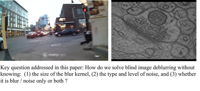
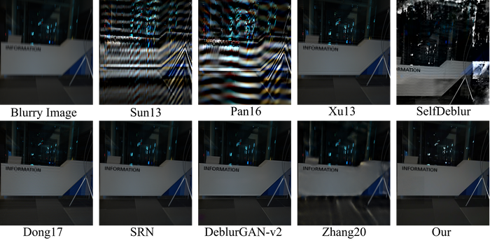
Image blur is mostly caused by the optical nonideality of the camera (e.g., defocus, lens distortion), i.e., optical blur, and relative motions between the scene and the camera, i.e., motion blur Szeliski2021Computer ; KundurHatzinakos1996Blind ; JoshiEtAl2008PSF ; LevinEtAl2011Understanding ; KoehlerEtAl2012Recording ; LaiEtAl2016Comparative ; KohEtAl2021Single ; SunDonoho2021Convex . It is often coupled with noticeable sensory noise, e.g. when one images fast-moving objects in low-light environments. Thus, in the simplest form, image blur is often modeled as

$$𝐲=𝐤\ast 𝐱+𝐧,$$ (1)

where $𝐲$ is the observed blurry and noisy image, and $𝐤$, $𝐱$, $𝐧$ are the blur kernel, clean image, and additive sensory noise, respectively. The notation $\ast$ here is linear convolution, which encodes the assumption that the blur effect is uniform over the spatial domain. When there are complicated 3D motions (e.g., multiple independently moving objects, and 3D in-plane rotations), or substantial depth variations, this model can be upgraded to account for the non-uniform blur effect LevinEtAl2011Understanding ; KoehlerEtAl2012Recording ; LaiEtAl2016Comparative ; KohEtAl2021Single . In this paper, we focus on the uniform setting and leave the non-uniform setting as future work.

Assume the model in Eq. 1. Given $𝐲$ and $𝐤$, estimating $𝐱$ is called (non-blind) deconvolution, a linear inverse problem that is relatively easy to solve. However, in practice, $𝐤$—including its size and numerical value—is often unavailable. For example, neither defocus nor motions can be reliably estimated in wild environments KundurHatzinakos1996Blind (see, e.g., Fig. 1). This leads to blind deconvolution (BD), where $𝐤$ and $𝐱$ are estimated together from $𝐲$.

Over the past decades, a rich set of ideas have been developed to tackle BID and BD, evolving from single-instance methods that rely on analytical processing or statistical inference and numerical optimization to solve one instance each time, to modern data-driven methods that aim to train deep learning (DL) models to solve all future instances. The sequence of landmark review articles KundurHatzinakos1996Blind ; LevinEtAl2011Understanding ; KoehlerEtAl2012Recording ; LaiEtAl2016Comparative ; KohEtAl2021Single ; ZhangEtAl2022Deep chronicle these developments; see also Section 2.1 below. Evaluation has also moved from synthetic to real-world data, best exemplified by the recent NTIRE 2020/2021 challenges on real-world image deblurring NahEtAl2020NTIRE ; NahEtAl2021NTIRE .

In this paper, we focus on single-instance methods for BID. Although recent data-driven methods have shown great promise, as statistical learning methods, they are intrinsically limited by the training data: if trained with sufficiently diverse and realistic data, these methods are likely to generalize well. However, the collection of high-quality training sets that meet the demand has been identified as a continuing challenge KohEtAl2021Single ; ZhangEtAl2022Deep . Therefore, single-instance methods will likely be a mainstay alongside data-driven methods for practical BID, especially for scenarios where relevant data are rare or expensive to collect.

Prior single-instance methods for BID seem vague on three critical issues toward practicality: (1) unknown kernel ($𝐤$) size: Except for methods that directly estimate $𝐱$ only (e.g., the inverse filtering approach to BD Wiggins1978Minimum ; Donoho1981MINIMUM ; Cabrelli1985Minimum ; SunDonoho2021Convex ), a nearly-optimal estimate of the kernel size is needed SiYaoEtAl2019Understanding . But it is practically unclear how such an accurate estimate can be reliably obtained, and how sensitive the existing methods are to kernel-size misspecification; (2) substantial noise ($𝐧$): Sensory noise after convolution may still be substantial, while most previous methods assume noise-free or low-noise settings in their evaluations TaiLin2012Motion ; ZhongEtAl2013Handling ; PanEtAl2016Robust ; DongEtAl2017Blind ; GongEtAl2017Self ; ChenEtAl2020OID ; and (3) model stability: The image may be blurry only, noisy only, or both. Whatever the case, in practice, an ideal BID method should work seamlessly across the different regimes. This has rarely been tested for prior methods. These three issues are summarized in Fig. 1.

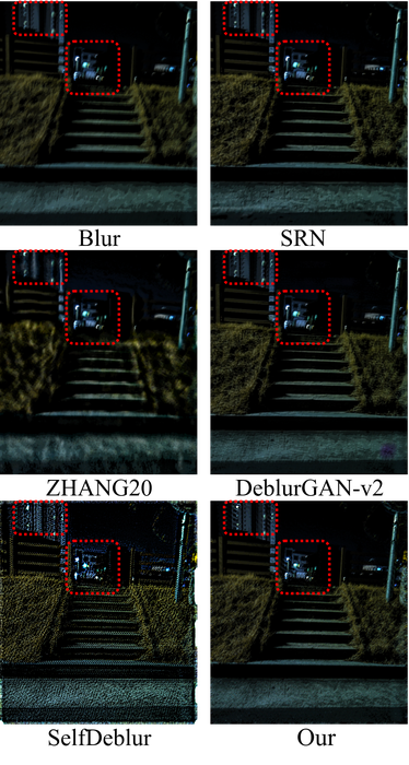
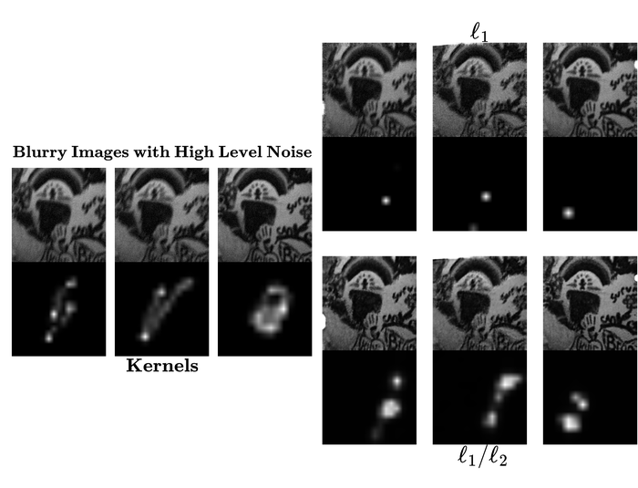
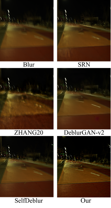
To quickly confirm these practicality issues, we pick $6$ state-of-the-art (SOTA) single-instance BID methods (plus $3$ representative data-driven methods by taking their pretrained models), and test them on a real-world image taken in a low-light setting, with unknown kernel size and unknown noise type/level. We specify a kernel size that is half of the image size in each dimension to provide a loose upper bound. Fig. 2 shows how miserably these single-instance methods can fail; more failures can be checked in Section 4.

This paper aims to address these practicality issues. We follow the major modeling ideas in the statistical inference and optimization approach to BID, but parametrize both the kernel and the image using trainable structured deep neural networks (DNNs). This idea has recently been independently introduced to BID by WangEtAl2019Image , RenEtAl2020Neural (SelfDeblur), and TranEtAl2021Explore , inspired by the remarkable success of deep image prior (DIP) UlyanovEtAl2020Deep and its variants HeckelHand2019Deep ; SitzmannEtAl2020Implicit in solving a variety of inverse problems in computer vision and imaging DarestaniHeckel2021Accelerated ; GandelsmanEtAl2019Double ; SitzmannEtAl2020Implicit ; TancikEtAl2020Fourier ; QayyumEtAl2021Untrained and beyond RavulaDimakis2019One ; MichelashviliWolf2019Speech . Our key contributions include

• identifying three practicality issues of SOTA single-instance BID methods, including SelfDeblur. As far as we are aware, this is the first time these three practicality issues have been discussed and addressed together in the BID literature. BID with these three issues is a more difficult but practical version than what SelfDeblur and most classical BID methods target. This is also the first time both classical and SOTA data-driven BID methods are systematically evaluated in the simultaneous presence of the three issues; see Section 3.1 and Section 4.2;

• revamping SelfDeblur with six crucial modifications to address the three issues. In Section 3.1, we clearly describe our modifications, as well as the rationale and intuitions behind them. Figuring out these modifications and their right combination is a highly nontrivial task, making our algorithm pipeline sufficiently different from SelfDeblur.

• systematic evaluation of our method against SOTA single-instance BID methods on synthetic SOTA datasets, and against SOTA data-driven BID methods on real world datasets, confirming the superior effectiveness and practicality of our method (Section 4; Fig. 2 gives a quick preview). We also pinpoint the failure modes and limitations of our method in Section 4.4.

2 Background

2.1 Blind deconvolution (BD)

BD refers to the nonlinear inverse problem of estimating $(𝐤,𝐱)$ from $𝐲$ according to the model in Eq. 1, and finds applications in numerous fields such as seismology Wiggins1978Minimum ; Donoho1981MINIMUM , digital communications VembuEtAl1994Convex ; DingLuo2000fast , neuroscience Lewicki1998review ; EkanadhamEtAl2011blind , microscopy CheungEtAl2020Dictionary , and computer vision.

Due to the bilinear mapping $(𝐤,𝐱)\mapsto 𝐤\ast 𝐱$, $(\delta ,𝐤\ast 𝐱)$ is always a trivial solution, where $\delta$ is the Dirac delta function. Therefore, without further restrictions to $𝐤$ and $𝐱$, recovery is hopeless. To ensure identifiability, different domain-specific priors have been proposed over time. A popularly used prior across these domains is that $𝐱$ is (approximately) “sparse” in an appropriate sense Wiggins1978Minimum ; Donoho1981MINIMUM ; Cabrelli1985Minimum ; SunDonoho2021Convex ; VembuEtAl1994Convex ; DingLuo2000fast ; Lewicki1998review ; EkanadhamEtAl2011blind ; CheungEtAl2020Dictionary . For BID, $𝐱$ as the natural image to be recovered is often assumed to be sparse in the gradient domain. Furthermore, $𝐤$ is often “short” or “small”, as characteristic patterns are often narrowly confined in their temporal or spatial extents Lewicki1998review ; EkanadhamEtAl2011blind ; CheungEtAl2020Dictionary . For BID, the blur kernel, either optical or motion, tends to be smaller in support, if not much, than the size of the blurry image itself. Therefore, the goal of many BD applications is to solve this short-and-sparse BD (SSBD).

Another notable feature of BD caused by the bilinear mapping $(𝐤,𝐱)\mapsto 𝐤\ast 𝐱$ is trivial symmetries. If we assume $𝐤$ and $𝐱$ are 1-dimensional infinite sequences—they can still have finite supports, then $𝐤\ast 𝐱=(\frac{1}{\alpha }{𝐤}_{-\tau })\ast (\alpha {𝐱}_{\tau })$ for any $\alpha \ne 0$ and $\tau \in \mathbb{Z}$, where ${𝐯}_{\tau }$ for any $𝐯$ means shifting $𝐯$ by $\tau$ time step. In other words, we have scale and shift symmetries. So, recovery is up to these symmetries, which often suffices for practical purposes. When we take a finite-window observation of $𝐤\ast 𝐱$, a more faithful model is

$$𝐲=𝒯\left(𝐤\ast 𝐱\right)+𝐧,$$ (2)

where $𝒯$ models the truncation effect of the window. The shift symmetry and the truncation effect together, if not handled appropriately, can easily lead to algorithmic failures, as discussed in Sections 3.1.1 and 3.1.2.

On the theoretical front, Donoho1981MINIMUM ; SunDonoho2021Convex ; ChoudharyMitra2014Sparse ; LiEtAl2015Unified ; LiEtAl2017Identifiability ; KechKrahmer2017Optimal discuss the identifiability of BD under different priors. For guaranteed recovery, AhmedEtAl2014Blind ; Chi2016Guaranteed ; LiEtAl2019Rapid assume $𝐤$ and/or $𝐱$ lying on random subspaces, and ZhangEtAl2017Global ; ZhangEtAl2020Structured ; KuoEtAl2020Geometry work on SSBD under certain probabilistic generative models on $𝐱$. In addition, WipfZhang2014Revisiting derives insights on different priors and formulations for BD from a Bayesian perspective.

2.2 BD specialized to blind image deblurring (BID)

For BID, SSBD is often solved with additional kernel- and/or image-specific priors. A subset of early BID methods write $𝐤$ in parametrized analytical forms, e.g., Gaussian shaped, and solve BID with simple analytical or computational steps KundurHatzinakos1996Blind . This has been largely superseded by the statistical inference and numerical optimization approach over the past decade, which formulates SSBD as regularized optimization problems, often interpreted as Maximum A Posterior (MAP) estimation:

$$\underset{𝐤,𝐱}{\min }\underset{\text{data fitting}}{\underbrace{\mathrm{\ell }\left(𝐲,𝐤\ast 𝐱\right)}}+\underset{\text{regularizing}𝐤}{\underbrace{{\lambda }_{𝐤}{R}_{𝐤}\left(𝐤\right)}}+\underset{\text{regularizing}𝐱}{\underbrace{{\lambda }_{𝐱}{R}_{𝐱}\left(𝐱\right)}},$$ (3)

where ${\lambda }_{𝐤},{\lambda }_{𝐱}$ are regularization parameters. A canonical choice is $\mathrm{\ell }\left(𝐲,𝐤\ast 𝐱\right)={\Vert 𝐲-𝐤\ast 𝐱\Vert }_2^2$, and $R_{𝐱}\left(𝐱\right)={\Vert \nabla 𝐱\Vert }_1$ (i.e., total-variation, or TV, norm on $𝐱$) to encode sparsity in the gradient. But since $𝐤\ast 𝐱=\left(\frac{1}{\alpha }𝐤\right)\ast (\alpha 𝐱)$ and ${\Vert \nabla (\alpha 𝐱)\Vert }_1=\left|\alpha \right|{\Vert \nabla 𝐱\Vert }_1$ for any $\alpha \ne 0$, without any further constraint the global solution is when $𝐱=\mathrm{𝟎}$. So a considerable chunk of recent research is about dealing with the scaling issue together with better sparsity encoding:

• $𝐤\ge \mathrm{𝟎},{\sum }_i{k}_i=1,R_{𝐱}\left(𝐱\right)={\Vert \nabla 𝐱\Vert }_1$: This is a classical remedy ChanWong1998Total , but is shown to prefer the trivial solution with $𝐤=\delta$ in certain regimes LevinEtAl2011Understanding . In fact, the trivial solution can occur even if one takes $R_{𝐱}\left(𝐱\right)={\Vert \nabla 𝐱\Vert }_q$ ($q\in (0,1]$), considerably tighter sparsity proxies. Nonetheless, perhaps surprisingly, carefully chosen algorithms can find nontrivial local solutions that lead to good recovery PerroneFavaro2014Total .

• $𝐤\ge \mathrm{𝟎},{\sum }_i{k}_i=1$, $R_{𝐱}\left(𝐱\right)=\frac{{\Vert \nabla 𝐱\Vert }_1}{{\Vert \nabla 𝐱\Vert }_2}$ or ${\Vert \nabla 𝐱\Vert }_0$: The high-level intuition why the above may prefer the trivial solution $\left(\delta ,𝐤\ast \nabla 𝐱\right)$ (assuming $𝐧=\mathrm{𝟎}$) is: when $𝐤$ is non-sparse and satisfies the simplex constraint (i.e., $𝐤\ge \mathrm{𝟎},{\sum }_i{k}_i=1$), $\nabla (𝐤\ast 𝐱)=𝐤\ast \nabla 𝐱$ tends to have higher sparsity level that of $\nabla 𝐱$ due to the potential smoothing effect of $𝐤$, but $𝐤\ast \nabla 𝐱$ has a lower numerical scaling than that of $\nabla 𝐱$. The latter tends to outweigh the former as $𝐤$ becomes sufficiently dense LevinEtAl2011Understanding ; BenichouxEtAl2013fundamental . So, a possible fix is to use scale-invariant sparsity measures such as ${\mathrm{\ell }}_1/{\mathrm{\ell }}_2$ KrishnanEtAl2011Blind ; HurleyRickard2009Comparing or (near) ${\mathrm{\ell }}_0$ XuEtAl2013Unnatural ; PanEtAl2014Deblurring ; WipfZhang2014Revisiting .

• ${\Vert 𝐤\Vert }_2=1$, $R_{𝐱}\left(𝐱\right)={\Vert \nabla 𝐱\Vert }_1$ or (near) ${\Vert \nabla 𝐱\Vert }_0$: Recently, it has been shown under different settings WipfZhang2014Revisiting ; ZhangEtAl2020Structured ; ZhangEtAl2017Global ; KuoEtAl2020Geometry ; JinEtAl2018Normalized that ${\mathrm{\ell }}_2$ normalization on $𝐤$ can change the optimization landscape and render true $(𝐤,𝐱)$ as a global solution, even with the scale-sensitive ${\Vert \nabla 𝐱\Vert }_1$. This is also related to the popularly used ${\mathrm{\ell }}_2$ regularization in $𝐤$, which can be understood as the penalty form of such a constraint XuEtAl2013Unnatural ; PanEtAl2014Deblurring ; PanEtAl2016Blind ; YanEtAl2017Image ; ChenEtAl2019Blind ; TranEtAl2021Explore .

• Other priors: Other image-specific priors, such as color prior JoshiEtAl2009Image , Markov-random-field prior KomodakisParagios2013MRF , patch recurrence prior MichaeliIrani2014Blind , dark channel prior PanEtAl2016Blind , extreme channel prior YanEtAl2017Image , local maximum gradient prior ChenEtAl2019Blind , also help encode extra image structures and break the issue with the trivial solution.

Another line of ideas works with the data-fitting loss ${\Vert \nabla 𝐲-𝐤\ast \nabla 𝐱\Vert }_2^2$, combined with the different priors and regularizers discussed above JoshiEtAl2008PSF ; ChoLee2009Fast ; XuJia2010Two ; SunEtAl2013Edge ; ZhongEtAl2013Handling ; FangEtAl2014Separable ; GongEtAl2016Blind ; ZhangEtAl2017Global ; ChoLee2017Convergence ; LiuEtAl2018Deblurring ; YangJi2019Variational . Most of them employ explicit edge detection and filtering to improve kernel estimation at initialization and during iteration, but edge processing can be sensitive to noise ZhongEtAl2013Handling ; GongEtAl2016Blind .

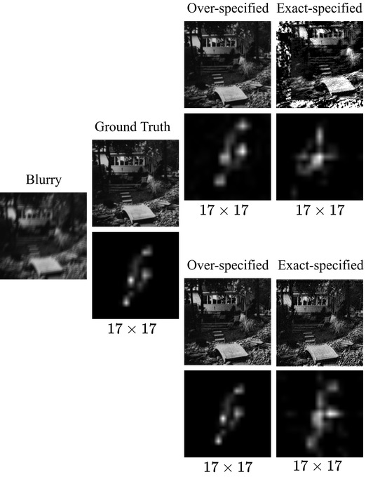
Almost all the existing single-instance methods accept a user-specified kernel size, hopefully a tight upper bound of the true size, as a problem hyperparameter. For synthetic datasets such as those released by LevinEtAl2011Understanding ; LaiEtAl2016Comparative , the “true” kernel sizes—which are in fact slightly over-specified kernel sizes, as shown in Fig. 3—are available. For real-world datasets, such as the real-world part of LaiEtAl2016Comparative and NahEtAl2020NTIRE , kernel sizes are unknown, and most prior work is vague about how they choose appropriate kernel sizes. We suspect that their selections are probably based on trial-and-error combined with visual inspection of the recovery quality.

Figure 3: Kernels from the synthetic datasets in LevinEtAl2011Understanding and LaiEtAl2016Comparative . Note that the true supports of the kernels are all slightly smaller than the specified kernel sizes, due to the presence of the black (zero) boundaries. Convention in the subcaptions: true size (specified size).

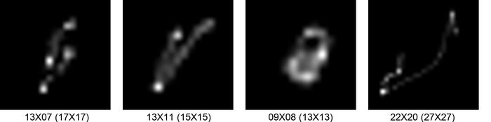
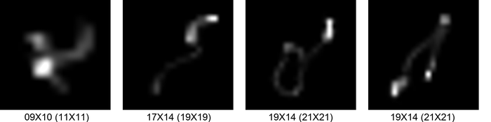
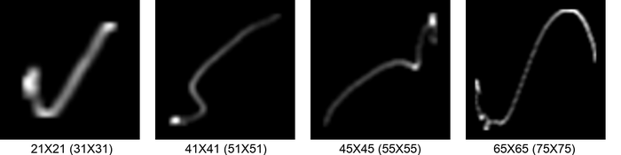
As far as we are aware, SiYaoEtAl2019Understanding is the first work explicitly addressing the kernel-size overspecification issue. They propose adding a low-rankness prior on the kernel: indeed, with increasing overspecification, the kernel becomes relatively sparse and low-rank, as is evident from Fig. 3.

Figure 4: Examples of blurry images with realistic noise. The clean image is taken from LaiEtAl2016Comparative ; the simulation of noise follows the procedure in HendrycksDietterich2019Benchmarking .

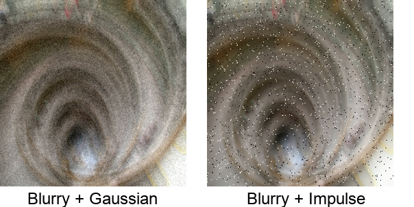
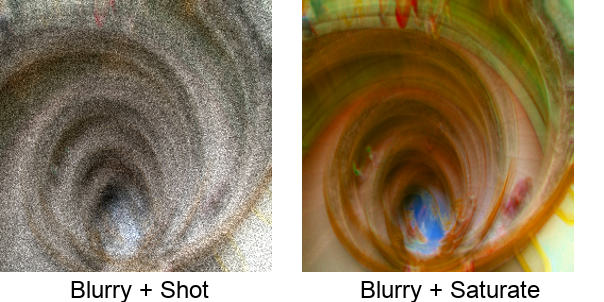
While early works test their methods on synthetic datasets with Gaussian noise (often with $\sigma =0.01$ following KrishnanFergus2009Fast ), only few papers have explicitly handled large, realistic noise, such as impulse/shot noise, or pixel saturation TaiLin2012Motion ; ZhongEtAl2013Handling ; PanEtAl2016Robust ; DongEtAl2017Blind ; GongEtAl2017Self ; ChenEtAl2020OID ; see examples in Fig. 4. In handling practical noise, a common thread is to learn or design a robust loss term $\mathrm{\ell }$ that is less sensitive to large/outlying pixel errors, e.g., by learning a pixel mask together with $𝐤$ and $𝐱$ ZhongEtAl2013Handling ; PanEtAl2016Robust ; GongEtAl2017Self ; ChenEtAl2020OID ; ChenEtAl2021Blind , or by using carefully-defined robust statistical losses DongEtAl2017Blind .

After 2015, data-driven DL-based methods for BID have emerged, targeting both the uniform and non-uniform settings. There are primarily two families of methods, parallel to those for solving linear inverse problems OngieEtAl2020Deep : 1) end-to-end approach. Deep neural networks (DNNs) are directly trained to predict the kernel, the sharp image or both. We refer the reader to the excellent surveys KohEtAl2021Single ; ZhangEtAl2022Deep , and the Github repository Vasu2021Image with an updated list of relevant papers; 2) hybrid approach. This includes many possibilities: DNNs are pretrained to model priors on $𝐤$ and $𝐱$ PanEtAl2021Physics ; AsimEtAl2020Blind ; LiEtAl2018Learning or to replace algorithmic components to solve Eq. 3 (i.e., plug-and-play methods, e.g. ZhangEtAl2019Deep ); DNNs are directly trained as components of unrolled numerical methods for solving Eq. 3 SchulerEtAl2016Learning ; AljadaanyEtAl2019Douglas ; LiEtAl2019Deep . Again, we recommend the two surveys and the Github repository for comprehensive coverage. These data-driven methods are apparently powered and meanwhile limited by the capacities of the training datasets used; the difficulty in constructing expressive and realistic training sets and, hence, poor generalization remain the key challenges KohEtAl2021Single .

2.3 Deep image prior (DIP) for BID

Deep image prior (DIP), as its name suggests, hypothesizes that natural images, or, in general, natural visual objects, can be parameterized as the output of trainable DNNs UlyanovEtAl2020Deep . Specifically, any visual object of interest, $𝒪$, is written as $𝒪=G_{\theta }(𝐳)$: $G_{\theta }$ is a structured DNN (often convolutional DNN to have a bias toward natural visual structures) that can be thought of as a generator, and $𝐳$ is the seed (i.e., input) to $G_{\theta }$. Often, $G_{\theta }$ is trainable and $𝐳$ is randomly initialized and then fixed.

Visual inverse problems (VIPs) involve estimating a visual object $𝒪$ from an observation $𝐲\approx f\left(𝒪\right)$, where $f$ models the observation (i.e., forward) process and the approximation sign $\approx$ indicates the potential existence of observational and modeling noise. Traditionally, VIPs are often posed as regularized data-fitting:

$$\underset{𝒪}{\min }\underset{\text{data fitting}}{\underbrace{\mathrm{\ell }\left(𝐲,f\left(𝒪\right)\right)}}+\underset{\text{regularizer}}{\underbrace{\lambda R\left(𝒪\right)}},$$ (4)

of which problem (3) is a specialization for SSBD. Imposing DIP onto $𝒪$ naturally leads to

$$\underset{\theta }{\min }\mathrm{\ell }\left(𝐲,f\circ G_{\theta }(𝐳)\right)+\lambda R\circ G_{\theta }(𝐳),$$ (5)

where $\circ$ denotes function composition, and the regularizer $R$ that encodes other priors is sometimes omitted. This simple idea has fueled surprisingly competitive methods for solving numerous computational vision and imaging tasks, ranging from basic image processing UlyanovEtAl2020Deep ; HeckelHand2019Deep ; HeckelSoltanolkotabi2019Denoising ; WangEtAl2019Image ; TranEtAl2021Explore , to advanced computational photography GandelsmanEtAl2019Double ; SitzmannEtAl2020Implicit ; TancikEtAl2020Fourier ; MaEtAl2021Unsupervised ; williams2019deep , and to sophisticated medical and scientific imaging applications DarestaniHeckel2021Accelerated ; LawrenceEtAl2020Phase ; BostanEtAl2020Deep ; TayalEtAl2021Phase ; ZhouHorstmeyer2020Diffraction ; ZhuangEtAl2022Practical ; see the recent survey QayyumEtAl2021Untrained .

Figure 5: Deblurring performance of SelfDeblur RenEtAl2020Neural and Explore TranEtAl2021Explore on blurry only (1st row), blurry and noisy (2nd row), and noisy only (3rd row) images. The noise, if present, is Gaussian noise with $\sigma =0.08$. The columns are the observed image (1st column), recovery result of SelfDeblur with exact specification of the kernel size, recovery result of SelfDeblur  with over specification of the kernel size, and recovery result of Explore with over specification of the kernel size, respectively. Note that the pretrained models from Explore allow only a fixed kernel size $64\times 64$.

When applying the DIP idea to BID, due to the asymmetric roles played by the kernel $𝐤$ and the image $𝐱$, it is natural to parameterize them separately following the Double-DIP idea GandelsmanEtAl2019Double to obtain:

$$\begin{array}{c}\underset{{\theta }_{𝐤},{\theta }_{𝐱}}{\min }\mathrm{\ell }\left(𝐲,G_{{\theta }_{𝐤}}({𝐳}_{𝐤})\ast G_{{\theta }_{𝐱}}({𝐳}_{𝐱})\right)+\hfill \\ \hfill {\lambda }_{𝐤}{R}_{𝐤}\circ G_{{\theta }_{𝐤}}({𝐳}_{𝐤})+{\lambda }_{𝐱}{R}_{𝐱}\circ G_{{\theta }_{𝐱}}({𝐳}_{𝐱}),\end{array}$$ (6)

i.e., DIP reformulation of problem (3). This is the exact recipe followed by two previous works WangEtAl2019Image ; RenEtAl2020Neural ; they differ by their choices of $G_{{\theta }_k}$ and $G_{{\theta }_x}$, as well as the regularizers $R_{𝐤}$ and $R_{𝐱}$. We focus on reviewing SelfDeblur  RenEtAl2020Neural here, as our method mostly builds on top of it and the evaluation in WangEtAl2019Image is very limited.

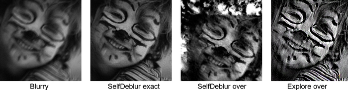
• RenEtAl2020Neural (SelfDeblur): $\mathrm{\ell }$ is the MSE. For the generators, $G_{{\theta }_{𝐱}}$ is convolutional U-Net similar to above, while $G_{{\theta }_{𝐤}}$ is a $2$-layer fully connected network. The disparate generators are to encode the asymmetry between the kernel and the image, and reflect the fact that the kernel tends to be much simpler than the image itself. Softmax and sigmoid final activations are then applied to $G_{{\theta }_{𝐤}}$ and $G_{{\theta }_{𝐱}}$, respectively. In addition, $R_{𝐱}$ is the classical TV regularizer that helps the method to work in the presence of low-level noise also. In summary,

  $\underset{{\theta }_{𝐤},{\theta }_{𝐱}}{\min }{\Vert 𝐲-G_{{\theta }_{𝐤}}({𝐳}_{𝐤})\ast G_{{\theta }_{𝐱}}({𝐳}_{𝐱})\Vert }_2^2$

  $+{\lambda }_{𝐱}{\Vert {\nabla }_{𝐱}{G}_{{\theta }_{𝐱}}({𝐳}_{𝐱})\Vert }_1,$ (7)

  $G_{{\theta }_{𝐤}}\text{:}2\text{-layer MLP, softmax final activation}$

  $G_{{\theta }_{𝐱}}\text{: conv. U-Net, sigmoid final activation}$

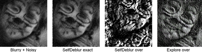
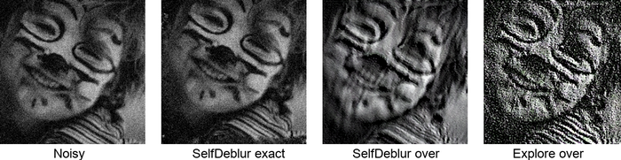
  From Fig. 5, it is evident that SelfDeblur works well only when $𝐲$ is blurry only and the kernel size is exactly specified. When there is considerable noise or the kernel-size is overspecified, SelfDeblur breaks down abruptly.

To move beyond the uniform blur model in Eq. 1 and construct a model that hopefully generalizes across different datasets, Explore TranEtAl2021Explore proposes learning an abstract blur operator $ℱ$ from a rich set of sharp-blurry image pairs. Once $ℱ$ is learned, for any given blurry image $𝐲$, the clean image $𝐱$ and the abstract kernel $𝐤$ are estimated via a generalized version of problem (6):

$$\begin{array}{c}\underset{{\theta }_{𝐤},{\theta }_{𝐱}}{\min }\mathrm{\ell }\left(𝐲,ℱ\left(G_{{\theta }_{𝐱}}({𝐳}_{𝐱}),G_{{\theta }_{𝐤}}({𝐳}_{𝐤})\right)\right)+\hfill \\ \hfill {\lambda }_{𝐤}{\Vert G_{{\theta }_{𝐤}}({𝐳}_{𝐤})\Vert }_2+{\lambda }_{𝐱}{\Vert \nabla G_{{\theta }_{𝐱}}({𝐳}_{𝐱})\Vert }_{2/3},\end{array}$$ (8)

Although Explore is a powerful and bold idea, but it is unclear if they really learn generalizable blur models, as well as if Eq. 8 is a good implementation of the double DIP idea. Our quick test shows that it does not work on a simple uniform blur case; see the $4$-th column of Fig. 5, especially when there is noise.

AsimEtAl2020Blind proposes three formulations for BID based on deep generative models in the same line of Eq. 6, but with pretrained generator(s). Since this method requires the pretrained kernel generator $G_{{\theta }_{𝐤}}$ from certain motion blur datasets, we will not compare with this method later.

None of the three DIP-for-BID works WangEtAl2019Image ; RenEtAl2020Neural ; TranEtAl2021Explore discussed above addresses the practicality issues around unknown kernel size, substantial noise, and model stability. Next, we propose several crucial modifications to SelfDeblur that tackle these issues altogether.

3 Our Method

Our method follows the double-DIP idea as formulated in Eq. 6, and builds on the two prior works WangEtAl2019Image and RenEtAl2020Neural (SelfDeblur), especially the latter. In Section 3.1, we describe six crucial ingredients of our method, and argue why they are necessary for the success. We then present our whole algorithm pipeline in Section 3.2.

3.1 Crucial ingredients

3.1.1 Overspecifying the size of $𝐤$

As we discussed in Section 2.2, most SOTA single-instance methods are evaluated on synthetic datasets, such as LevinEtAl2011Understanding and LaiEtAl2016Comparative , where reasonably tight upper bounds of kernel sizes are available. However, on more realistic datasets such as NahEtAl2020NTIRE ; NahEtAl2021NTIRE ; RimEtAl2020Real and particularly in real-world applications, no such tight bounds are available.

Figure 6: Illustration of the problem with under-specification of the kernel size. We take SelfDeblur (top group) and our method (bottom group; details in Section 3.2) with different kernel-size specifications ($7\times 7$, $17\times 17$, $27\times 27$, respectively), in contrast to the “true”—we estimate by locating the nonzero support of the kernel—kernel-size $23\times 21$.

In general, recovering $𝐤$ is not possible when the kernel size is underspecified. In fact, recovery of $𝐱$ is also not possible in this situation; consider the following argument for 1D cases.

Example 1

Assume that $𝐤\in {ℝ}^3$, $𝐱\in {ℝ}^5$, and $𝐲\in {ℝ}^5$ due to truncation. So

(9)

Now, suppose that the kernel size is specified as $2$ and also $𝐱$ is correctly recovered with a kernel estimate ${𝐤}^{\prime }\in {ℝ}^2$. Then, depending on the convention of the truncation, one of following products

(10)

should reproduce $𝐲$. But for generic $𝐱$, the matrix ${𝐌}_{𝐱}$ is column full-rank and hence $𝐲$ lies in the $3$-dimensional column space of ${𝐌}_{𝐱}$, i.e., $\mathrm{col}({𝐌}_{𝐱})$. Both products in Eq. 10 can fail to reproduce $𝐲$, as they produce points in $2$-dimensional subspaces of $\mathrm{col}({𝐌}_{𝐱})$ only. Due to the contradiction, recovery of $𝐱$ is generally not possible with the length-$2$ kernel specification.

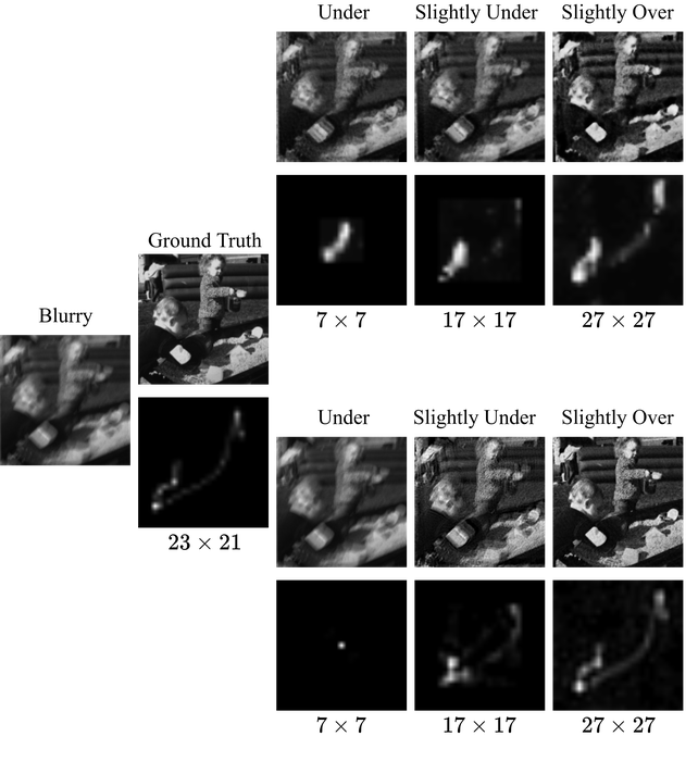
Indeed, as shown in Fig. 6, when the kernel is significantly under-specified, the estimated kernel is disparate from the true kernel. When the under-specification is slight, we can at best recover part of the true kernel. In both cases, the estimated images are still blurry to different degrees.

On the other hand, Fig. 6 also shows that with slight kernel-size overspecification, we manage to estimate the kernel and image with reasonably good quality. In theory, overspecification at least allows the possibility of the recovering the kernel padded with zeros. However, shortness of the kernel is also crucial in SSBD. Intuitively, when overspecification is substantial, there may be a fundamental identifiability issue, i.e., it is likely that $𝐲=𝒯\left(𝐤\ast 𝐱\right)=𝒯\left({𝐤}^{\prime }\ast {𝐱}^{\prime }\right)$ for a ${𝐤}^{\prime }$ that is substantially larger in size than $𝐤$, where $𝒯$ is the truncation operator defined in Eq. 2. So the question is what level of overspecification is safe: small enough to avoid the potential identifiability issue, while large enough to allow typical blur kernels.

Figure 7: Cumulative distribution function (CDF) of pixel-wise gradient norms over typical natural images. This is estimated from $234$ images randomly sampled from the RealBlur dataset RimEtAl2020Real . For each image, we obtain the gradient map by convolving the image with the standard Sobel filter. After calculating the pixel-wise ${\mathrm{\ell }}_2$ norms, we normalize these values into $[0,1]$ by dividing using the largest value and then estimate the CDF. The blue curve is the mean CDF and the shallow region indicates the standard deviation over the $234$ images.

Regarding the identifiability of SSBD with the model $𝐲=𝐤\ast 𝐳$ where $𝐳$ is sparse with respect to the canonical basis, ChoudharyMitra2014Sparse presents a strong negative result: for all $n_{𝐤},n_{𝐳}\ge 5$, there always exist non-identifiable pairs for any sparsity pattern assumed on $𝐳$ (distilled from their Section III.B and Theorem 2); ChoudharyMitra2018Properties provides a more quantitative version of the result (Theorem 3). Unfortunately, it remains open up to date if these non-identifiable cases are rare events. Nonetheless, all existing identifiability results based on other assumptions on $𝐤$ and $𝐳$ (particularly subspace-constrained and subspace-sparse assumptions as in LiEtAl2017Identifiability ; KechKrahmer2017Optimal ) roughly state that

$$\mathrm{DoF}\left(𝐲\right)\ge \mathrm{DoF}\left(𝐤\right)+\mathrm{DoF}\left(𝐳\right)$$ (11)

is the identifiability limit, where $\mathrm{DoF}$ stands for degrees of freedom. For SSBD, this can be mapped to

$$\mathrm{SIZE}\left(𝐲\right)\ge \mathrm{SIZE}\left(𝐤\right)+\mathrm{NNZ}\left(𝐳\right),$$ (12)

where $\mathrm{NNZ}$ denotes the number of non-zeros. For BID, $\nabla 𝐱$ is assumed to be sparse, we thus have

$$\mathrm{SIZE}\left(𝐲\right)\ge \mathrm{SIZE}\left(𝐤\right)+\mathrm{NNZ}\left(\left|\nabla 𝐱\right|\right),$$ (13)

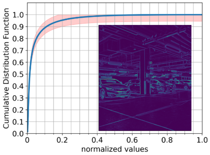
where $\left|\nabla 𝐱\right|$ denotes the element-wise gradient magnitude for image $𝐱$. So Eq. 13 tells us that a reasonable upper bound for kernel size depends on the typical sparsity level of gradient norms of natural images that we deal with in BID.

Fig. 7 provides the mean cumulative distribution function estimated over a subset of natural images from the RealBlur dataset RimEtAl2020Real . On average, $80\%$ of the gradient norms are below $5\%$ of the largest gradient norm, and $50\%$ below $1\%$ of the largest gradient norm. So if we set $1\%$ as the cutoff threshold, the numerical sparsity level of $\left|\nabla 𝐱\right|$ is below $0.5$, i.e., no more than half of the pixel values are nonzero after the cutoff. Thus, we over-specify the size of $𝐤$ as half of the size of $𝐲$ in both directions. This is a safe choice: if we allow extremely “thin” images and kernels consisting of single columns only, this still allows recovery. For general rectangular images and kernels, we could be slightly more aggressive in the over-specification. As far as we are aware, our setting represents the first time that the kernel size has been set in this “aggressive” regime.

3.1.2 Overspecifying the size of $𝐱$

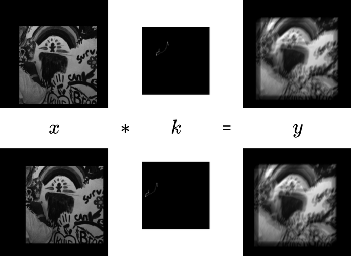
Suppose that $𝐤\in {ℝ}^{n_{𝐤}\times m_{𝐤}}$ and $𝐲\in {ℝ}^{n_{𝐲}\times m_{𝐲}}$. By the truncated linear convolution model of Eq. 2 (illustrated in Fig. 8), the part of $𝐱$ that can contribute to the values of $𝐲$ has a size of

$$\left(n_{𝐤}+n_{𝐲}-1\right)\times \left(m_{𝐤}+m_{𝐲}-1\right),$$ (14)

which is the appropriate size that we should specify for $𝐱$. Physically, underspecification, e.g., specifying the size of $𝐱$ identical to that of $𝐲$ is likely to lead to recovery failures, as illustrated in Figs. 8 and 9.

Figure 8: Illustration of the truncated linear convolution, and the necessity of appropriately specifying the size of $𝐱$. The black dashed box delineates the actual field of view (FOV) of the camera; the left column is the clean image, and the right the blurry image due to the horizontal $S$-shaped blur kernel. Note that inside the enlarged window of the blurry image, there are “ghost” branches from outside the FOV. Hence, if we specify the size of $𝐱$ exactly as the FOV, we are not able to recovery the clean scene inside the FOV due to the “ghost” visual components near the four boundaries.

Figure 9: Illustration of the necessity of overspecifying the size of $𝐱$. We take SelfDeblur (top group) and our method (bottom group; details in Section 3.2). The kernel size is specified as $17\times 17$, slightly larger than the actual size $15\times 11$ for both methods. In the over-specified cases, the size of $𝐱$ is specified as $(n_{𝐤}+n_{𝐲}-1)\times (m_{𝐤}+m_{𝐲}-1)$. In the exactly-specified cases, the size of $𝐱$ is specified as $n_{𝐲}\times m_{𝐲}$. Both methods return reasonable kernel and image estimates when the size of $𝐱$ is overspecified, and both produce estimates with visible artifacts when the size of $𝐱$ is exactly-specified—the artifacts by SelfDeblur are significant.

While the majority of previous works follow Eq. 14 in specifying the size of $𝐱$, e.g., SunEtAl2013Edge , PanEtAl2016Blind , DongEtAl2017Blind , and SelfDeblur  RenEtAl2020Neural , a small number of them set the size of $𝐱$ same as that of $𝐲$, e.g., XuEtAl2013Unnatural ) and Explore  TranEtAl2021Explore . We follow Eq. 14 in our setting.

Figure 10: Illustration of the bounded shift effect (top group), and the issue caused by central cropping as implemented in SelfDeblur (bottom group). Due to the simultaneous over-specification of the kernel and image sizes, the kernel and the image contents (i.e., the nonzero parts) can shift in opposite directions in ${ℝ}^2$—so long as they do not shift outside the boundaries, that leads to equivalent $\left(𝐤,𝐱\right)$ pairs to produce the same blurry image $𝐲$. Due to the uncertainty of the locations of kernel and image contents, central cropping (which is used in SelfDeblur) may include estimation noise from the background, as indicated by the red cropping boxes.

However, we do not know $n_{𝐤}$ and $m_{𝐤}$ exactly. By our overspecification strategy for $𝐤$ described in Section 3.1.1, the actual size we use, i.e., $\lceil \frac{1}{2}{n}_{𝐲}\rceil \times \lceil \frac{1}{2}{m}_{𝐲}\rceil$, can be substantially larger than $n_{𝐤}\times m_{𝐤}$. So the size we specify for $𝐱$ now becomes

$$(\lceil \frac{1}{2}{n}_{𝐲}\rceil +n_{𝐲}-1)\times (\lceil \frac{1}{2}{m}_{𝐲}\rceil +m_{𝐲}-1).$$ (15)

The simultaneous overspecification of $𝐤$ and $𝐱$ causes another problem: the bounded shift effect.

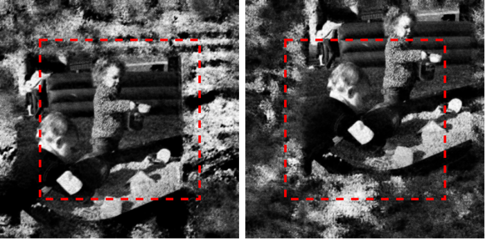
Recall that if $𝐤$ and $𝐱$ are 1-D infinite sequences, $𝐤\ast 𝐱=\left(\frac{1}{\alpha }{𝐤}_{-\tau }\right)\ast \left(\alpha {𝐱}_{\tau }\right)$ for all $\alpha \ne 0$ and $\tau \in \mathbb{Z}$. In other words, there are both scale and shift ambiguities if we want to recover $𝐤$ and $𝐱$ from $𝐲=𝐤\ast 𝐱$. There are similar ambiguities for 2-D $𝐤$ and $𝐱$ for BID. With the truncated convolution model of Eq. 2 on finite sequences, we do not have the shift ambiguity if the size of either $𝐤$ or $𝐱$ is exactly-specified. But, when both sizes are over-specified as we propose here, we expect the bounded shift ambiguity, as shown in Fig. 10: even if we successfully recover $𝐤$ and $𝐱$, their contents are embedded, not necessarily centered, in the larger background regions that we overspecify.

So we need a post-processing step to locate the contents of $𝐤$ and $𝐱$ after we obtain the overspecified versions of both; we propose an effective post-processing step in Section 3.1.6. We note that SelfDeblur uses the same $\left(n_{𝐲}+n_{𝐤}-1\right)\times \left(m_{𝐲}+m_{𝐤}-1\right)$ rule as ours to overspecify the size of $𝐱$, but their ${𝐧}_{𝐤}\times {𝐦}_{𝐤}$ is close to the true kernel size as they mostly evaluate only on synthetic data. Thus, the bounded shift ambiguity is not quite visible, and they simply centrally crop $𝐱$ to obtain the final estimated image. Once we move to real-world images where substantial overspecification of the kernel size is unavoidable, the central cropping strategy may cut out part of the image content augmented with non-physical estimation noise, as we show in Fig. 10.

3.1.3 The loss and regularizers

As summarized in • ‣ Section 2.3, SelfDeblur uses the standard MSE loss $\mathrm{\ell }$ and TV regularization, i.e., $R\left(𝐱\right)={\Vert {\nabla }_{𝐱}{G}_{{\theta }_{𝐱}}({𝐳}_{𝐱})\Vert }_1$. Here, we propose changing both the loss and the regularizer to make the method effective and robust even in the presence of substantial noise that may be beyond Gaussian.

For the loss, we switch to the famous Huber loss Huber1964Robust

(16)

The Huber loss penalizes less of large values compared to the MSE, and hence in regression problems the overall loss becomes less dominated by large errors. This implies that the regression models estimated from Huber loss minimization be less sensitive to outlying data points that tend to cause large regression errors. For BID, outlying pixels could be caused by, e.g., large noise (e.g., shot noise) and pixel saturation. This choice enables our method to work beyond the regime of low-level Gaussian noise that the majority of previous works, including SelfDeblur, have focused on.

Figure 11: Landscapes of different surrogates for the ${\mathrm{\ell }}_0$ function on ${ℝ}^2$. The normalized metrics ${\mathrm{\ell }}_p/{\mathrm{\ell }}_2$ are uniformly closer to ${\mathrm{\ell }}_0$ than their unnormalized counterparts—${\mathrm{\ell }}_p$ norms where $p\in (0,1]$. The approximation of ${\mathrm{\ell }}_p/{\mathrm{\ell }}_2$ to ${\mathrm{\ell }}_0$ becomes increasingly sharper as $p$ goes down to $0$.

Table 1: Performance of ${\mathrm{\ell }}_1/{\mathrm{\ell }}_2$ vs ${\mathrm{\ell }}_1$ as regularization with the optimal regularization parameter ${\lambda }_{𝐱}$’s. We take all test cases from the Levin dataset, and for each image, we search for the best ${\lambda }_{𝐱}$ (in terms of best peak PSNR) over the selections: $1$, $5\mathrm{e}-1$, $2\mathrm{e}-1$, $1\mathrm{e}-1$, $5\mathrm{e}-2$, $2\mathrm{e}-2$, $1\mathrm{e}-2$, $5\mathrm{e}-3$, $2\mathrm{e}-3$, $1\mathrm{e}-3$, $5\mathrm{e}-4$, $2\mathrm{e}-4$, $1\mathrm{e}-4$, $5\mathrm{e}-5$, $2\mathrm{e}-5$, $1\mathrm{e}-5$ for ${\mathrm{\ell }}_1/{\mathrm{\ell }}_2$ and ${\mathrm{\ell }}_1$ regularizers, respectively. We report the mean peak PNSRs and mean ${\lambda }_{𝐱}$’s (and the standard deviations inside parentheses) over the whole dataset for both low-level ($\sigma =1\mathrm{e}-3$) and high-level ($\sigma =5\mathrm{e}-2$) Gaussian noise.

	Low Level		High Level
	PSNR	$\lambda$	PSNR	$\lambda$
${\mathrm{\ell }}_1/{\mathrm{\ell }}_2$	32.64 (0.69)	0.0001 (0.018)	27.74 (0.23)	0.0002 (0.0019)
${\mathrm{\ell }}_1$	31.12 (0.52)	0.002 (0.07)	24.34 (0.78)	0.02 (0.10)

Figure 12: Illustration of the benefit of ${\mathrm{\ell }}_1/{\mathrm{\ell }}_2$ over ${\mathrm{\ell }}_1$ in avoiding trivial solutions in the high-noise regime (Gaussian noise with $\sigma =0.1$). Left: blurry and noisy images with their corresponding kernels; Right-Top: recovered images and kernels with ${\mathrm{\ell }}_1$ regularization; Right-Bottom: recovered images and kernels with ${\mathrm{\ell }}_1/{\mathrm{\ell }}_2$ regularization. The ${\mathrm{\ell }}_1$ regularization leads to single-blob kernel estimates that resemble the trivial $\delta$ function, and the estimated images are also similar to the original blurry and noisy images. In contrast, the recovered images from the ${\mathrm{\ell }}_1/{\mathrm{\ell }}_2$ regularization are much sharper.

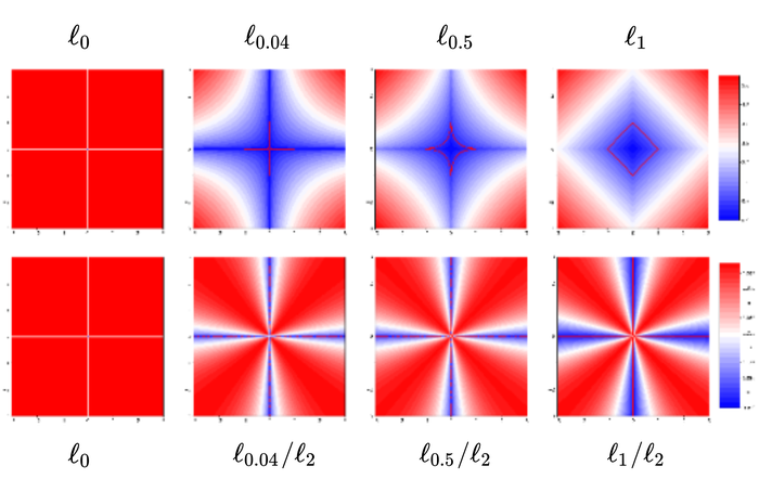
For the regularizer, we choose the ${\mathrm{\ell }}_1/{\mathrm{\ell }}_2$ version

$$R\left(𝐱\right)=\frac{{\Vert {\nabla }_{𝐱}{G}_{{\theta }_{𝐱}}({𝐳}_{𝐱})\Vert }_1}{{\Vert {\nabla }_{𝐱}{G}_{{\theta }_{𝐱}}({𝐳}_{𝐱})\Vert }_2}$$ (17)

for three reasons/benefits: 1) scaling invariance and perturbation robustness. To encode the sparsity prior on $\nabla 𝐱$, a natural choice is the ${\mathrm{\ell }}_0$ function, which is scale-invariant but sensitive to perturbations. ${\mathrm{\ell }}_1$ is a popular surrogate for ${\mathrm{\ell }}_0$ and robust to perturbations, but is scale equivariant. ${\mathrm{\ell }}_1/{\mathrm{\ell }}_2$ is scale-invariant and robust to small perturbations. Fig. 11 visualizes the differences between these functions; 2) insensitivity of the estimation performance to the regularization parameter ${\lambda }_{𝐱}$. Empirically, we find that with ${\mathrm{\ell }}_1/{\mathrm{\ell }}_2$ regularizer we can fix the ${\lambda }_{𝐱}$ level to obtain good performance across low- and high-level Gaussian noise, whereas the ${\mathrm{\ell }}_1$ regularizer requires setting ${\lambda }_{𝐱}$ to different orders of magnitude across different noise levels for good performance. Moreover, ${\mathrm{\ell }}_1/{\mathrm{\ell }}_2$ regularization leads to consistently superior performance. Details are included in Table 1; and 3) avoiding trivial solutions. As reviewed in Section 2.2, the original motivation of replacing the ${\mathrm{\ell }}_1$ with ${\mathrm{\ell }}_1/{\mathrm{\ell }}_2$ is to avoid the trivial solution $𝐤=\delta$ when using the simplex normalization on $𝐤$ KrishnanEtAl2011Blind . Although the simplex normalization is still used in SelfDeblur, the “double-DIP” parametrization together with gradient descent can potentially impose additional structural biases. So, a priori, it is unclear if we still need to worry about finding the trivial solution. Fig. 12 shows this concern remains: when the blurry images are also substantially noisy, the ${\mathrm{\ell }}_1$ regularizer tends to produce single-blob estimates that resemble finite-supported $\delta$ functions coupled with blurry image estimates. In contrast, the ${\mathrm{\ell }}_1/{\mathrm{\ell }}_2$ regularizer leads to much cleaner images, and also kernels that at least capture certain aspects of the groundtruth kernels.

3.1.4 The DIP models

Figure 13: Evolution of DIP, DIP-MLP, and SIREN representation of kernels during kernel estimation. Top: simple regression of a motion blur kernel, i.e., ${\min }_{\widehat{𝐤}}{\Vert 𝐤-\widehat{𝐤}\Vert }_2^2$ where $\widehat{𝐤}$ is the estimated kernel represented by each of the three models; Bottom: non-blind kernel estimation, i.e., ${\min }_{\widehat{𝐤}}{\Vert 𝐲-\widehat{𝐤}\ast 𝐱\Vert }_2^2$ where again $\widehat{𝐤}$ is the estimated kernel represented by each of the three models, and $𝐲$ and $𝐱$ are known. To evaluate the progress of each setting, we calculate the frequency band error (FBE), inspired by the frequency band correspondence (FBC) in ShiEtAl2022Measuring : For each setting, we calculate the point-wise relative estimation error over the Fourier domain $|ℱ(𝐤)-ℱ(\widehat{𝐤})|/|ℱ(𝐤)|$, and then divide the Fourier frequencies into five bands radially (the same division used in ShiEtAl2022Measuring ) and compute the per-band average. We term this metric frequency band error (FBE), and plot the evolution of the FBEs of all five frequency bands against the optimization iteration. It is evident that in both kernel estimation settings, SIREN recovers all frequency bands much faster and reliably than DIP and DIP-MLP.

Figure 14: Performance of different model combinations for $(𝐤,𝐱)$. Top: with low Gaussian noise ($\sigma =0.001$); Bottom: with high Gaussian noise ($\sigma =0.05$). Our combination, DIP (for $𝐱$) + SIREN (for $𝐤$), leads to more faithful kernel and image estimation in both low- and high-noise regimes that DIP+DIP (as in WangEtAl2019Image ) and DIP+DIP-MLP (as in SelfDeblur). For fair comparison, we only change the model combination and leave all other settings as our default.

Figure 15: Performance of the DIP+DIP-MLP (as in SelfDeblur) and DIP+SIREN (ours) model combinations for a noisy image (Gaussian with $\sigma =0.1$) without blur. The DIP+SIREN combination leads to sharper estimation of the image compared to DIP+DIP-MLP. For fair comparison, we only change the model combination and leave all other settings as our default.

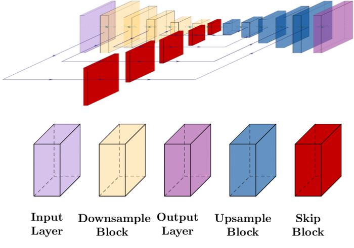
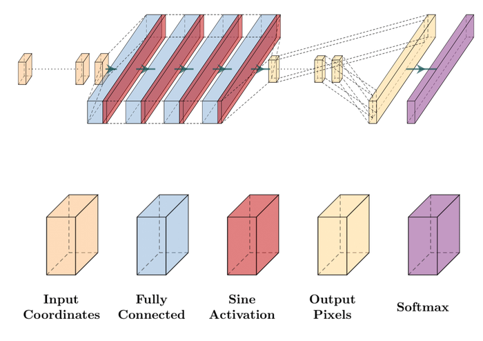
As discussed around Eq. 6 and detailed in the DNN choices in • ‣ Sections 2.3 and 8, the DIP models to parameterize $𝐤$ and $𝐱$ should encode the right structural priors for them and reflect the asymmetry between $𝐤$ and $𝐱$. Same as SelfDeblur, we choose a convolutional U-Net $G_{\theta }$ for $𝐱$. For $𝐤$, we choose the sinusoidal representation networks (SIREN) SitzmannEtAl2020Implicit over the MLP architecture used in SelfDeblur.

Same as DIP, SIREN also parametrizes visual objects using DNNs. Unlike DIP where the DNN outputs the visual object, in SIREN the DNN represents the visual object itself. For example, SIREN models a continuous grayscale image as $ℐ:{[0,1]}^2\mapsto ℝ$, i.e., a real-valued function on the compact domain ${[0,1]}^2\subset {ℝ}^2$, and then produces a finite-resolution version of $ℐ$ via discretization. The DNN in SIREN is a modified MLP architecture that takes two coordinate inputs and returns a single value (for grayscale image) or three values (for RGB images).

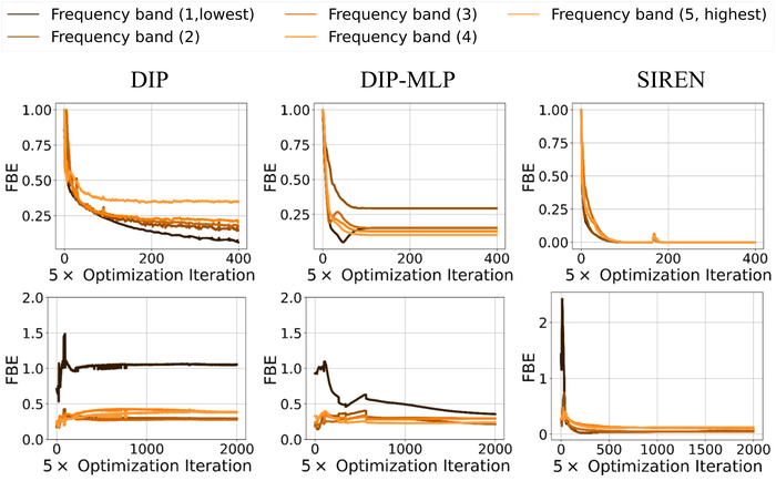
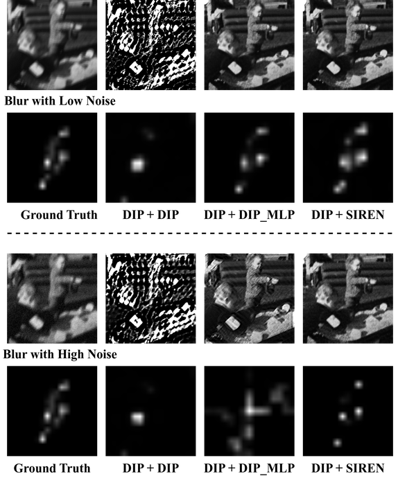
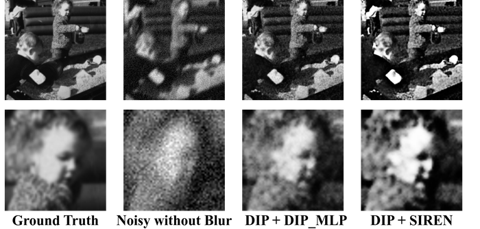
Practical blur kernels can have substantial high-frequent components in the Fourier domain, e.g., most motion blur kernels that consist of convoluted curves (see Fig. 3), and narrow Gaussian-shaped defocus kernels. The reason for choosing SIREN over DIP to represent $𝐤$ is that SIREN and similar coordinate encoding networks are empirically observed to learn high-frequency components of visual objects better than DIP SitzmannEtAl2020Implicit ; TancikEtAl2020Fourier ; see also Footnote 6, where we show quantitatively that on two simplified kernel estimation problems, SIREN allows recovering all frequency bands, particularly the high frequency band, of the true kernel much more efficiently and reliably than DIP with the default encoder-decoder (dubbed as DIP) and with the MLP architecture (dubbed as DIP-MLP) for $G_{\theta }$. When we plug SIREN into BID, the DIP (for $𝐱$)+SIREN (for $𝐤$) model combination easily outperforms other combinations, i.e., DIP+DIP (as in WangEtAl2019Image ) and DIP+DIP-MLP (as in SelfDeblur), especially when substantial noise is present, as shown in Fig. 14. Moreover, we also observe the benefit of SIREN in terms of improving the model stability: Fig. 15 shows that when the image is only contaminated by high noise, the DIP+SIREN combination tends to return a sharper image estimate than that of DIP+DIP-MLP.

3.1.5 Early stopping (ES)

Figure 16: Illustration of the overfitting issue of SelfDeblur with the setting in (• ‣ 2.3). The estimation quality of $𝐱$ first climbs to a peak and then plunges due to overfitting to the noise. The early stopping (ES) method for DIP developed in our prior paper WangEtAl2021Early can successfully detect stopping points that lead to near-peak performance.

Figure 17: PSNR curves of our method on $(𝐤,𝐱)$ reconstruction with different regularization parameters (Gaussian noise with $\sigma =0.05$). Overfitting is persistent across the different regularization levels. Moreover, the peak iterations of $𝐤$ and $𝐱$ curves for each $\lambda$ are roughly equationed, and so we only use the $𝐱$ curves for ES detection.

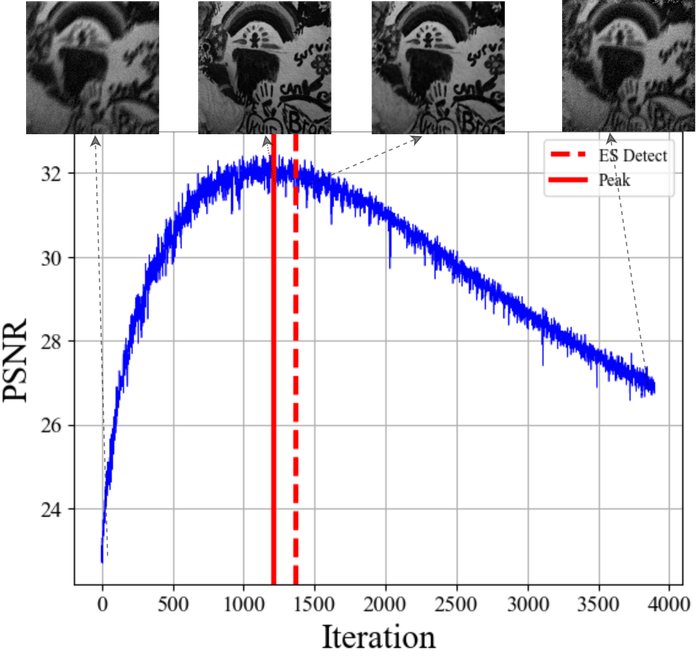
Besides the three common practicality issues for BID that we have addressed so far, there is one more specific to the double-DIP approach: overfitting. As shown in Fig. 16, the estimation quality (measured by PSNR with respect to the groundtruth image $𝐱$) of SelfDeblur  first climbs to a peak and then degrades as the iteration goes on.

To understand what happens here, we can think about the double-DIP loss itself:

$$\mathrm{\ell }\left(𝐲,G_{{\theta }_{𝐤}}({𝐳}_{𝐤})\ast G_{{\theta }_{𝐱}}({𝐳}_{𝐱})\right)$$ (18)

from Eq. 6. In practice, the image $𝐲$ is both blurry and noisy, and the DIP models $G_{{\theta }_{𝐤}}({𝐳}_{𝐤})$ and $G_{{\theta }_{𝐱}}({𝐳}_{𝐱})$ are substantially overparametrized. So if we perform global optimization, $𝐲=G_{{\theta }_{𝐤}}({𝐳}_{𝐤})\ast G_{{\theta }_{𝐱}}({𝐳}_{𝐱})$ for typical losses, such as MSE. Thus, the final $G_{{\theta }_{𝐱}}({𝐳}_{𝐱})$ likely accounts for noise also besides the desired image content, which leads to the final quality degradation. The bell-shaped quality curve is explained by the implicit bias of first-order optimization methods used to perform the loss minimization: over-parametrized DNN models trained with first-order methods tend to learn structured visual contents much faster than learn unstructured noise; see HeckelSoltanolkotabi2020Compressive and HeckelSoltanolkotabi2019Denoising for complete theories on simplified models. The previous double-DIP-based works WangEtAl2019Image , SelfDeblur RenEtAl2020Neural , Explore TranEtAl2021Explore do not address this issue, as they work with negligible noise levels that avoid the overfitting. To deal with practical noise that can be substantial, we need to address it in this paper.

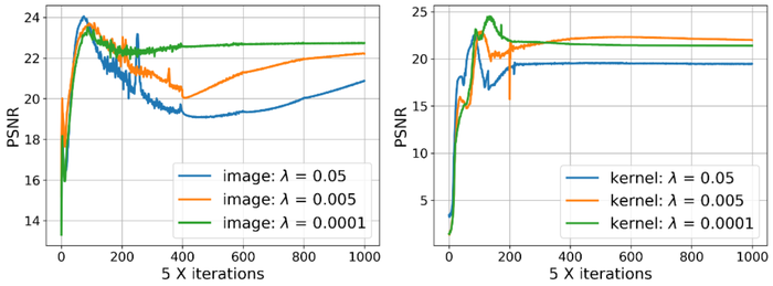
To get a good reconstruction, we can either control the DNN capacities by proper regularization, or stop the iteration early around the peak performance—early stopping (ES); see our prior works LiEtAl2021Self and WangEtAl2021Early for summaries of related work. We have shown in the couple of papers that the regularization strategy suffers from serious practicality issues; Fig. 17 shows that overfitting is persistent across different levels of regularization (with our choice of ${\mathrm{\ell }}_1/{\mathrm{\ell }}_2$ regularizer as detailed above). So, we advocate ES-based solution instead, and adopt the windowed-moving-variance-based ES (WMV-ES) method developed in WangEtAl2021Early that proves effective and lightweight for DIP and its variants on numerous application scenarios. As the name suggests, WMV-ES calculates the windowed moving variance curve of the intermediate reconstructions, and detects the first major valley of the WMV curve as the recommended ES point. For our purpose, we observe that the $𝐤$ and $𝐱$ PSNR curves are often automatically “synchronized” and reach the peaks roughly around the same iteration. Thus, we only keep track of reconstructed images, not the kernels. Fig. 16 shows this simple method can effectively detect a near-peak stopping point with little loss of the reconstruction quality.

3.1.6 Post-processing to locate $\widehat{𝐱}$

As discussed in Section 3.1.2 and illustrated in Fig. 10, the simultaneous overspecification of the sizes of $𝐤$ and $𝐱$ leads to the bounded shift effect on $𝐤$ and $𝐱$, and hence the estimated $𝐤$ and $𝐱$ may not be centered. So we need an algorithm to automatically locate the estimated image $\widehat{𝐱}$, assumed of the same size as $𝐲$. Once we can locate $\widehat{𝐱}$ and thereof estimate the shift from the center, we can use shift-symmetry between $𝐤$ and $𝐱$ to locate $\widehat{𝐤}$ also if desired.

To locate $\widehat{𝐱}$, we propose a simple sliding-window strategy: we use the noisy and blurry image $𝐲$ as a template, and slide it across the output, overspecified image from $G_{{\theta }_{𝐱}}$. The similarity of each of windowed patch from $G_{{\theta }_{𝐱}}$ and $𝐲$ is calculated using structural similarity index measure (SSIM) to emphasize the perceptual nearness, and the patch with the largest SSIM value is eventually extracted as $\widehat{𝐱}$.

3.2 Our algorithm pipeline

Algorithm 1 BID with unknown kernel size and substantial noise (uniform kernel)

1:blurry and noisy image $𝐲$, kernel size $n_{𝐤}\times m_{𝐤}$ (default: $\lceil n_{𝐲}/2\rceil \times \lceil m_{𝐲}/2\rceil$), random seed ${𝐳}_{𝐱}$ for $𝐱$, randomly initialized network weights ${\theta }_{𝐤}^{(0)}$ and ${\theta }_{𝐱}^{(0)}$, optimal image estimate ${𝐱}^{\ast }=G_{{\theta }_{𝐱}^{(0)}}({𝐳}_{𝐱})$, regularization parameter ${\lambda }_{𝐱}$, iteration index $i=1$, WMV-ES window size $W=100$, WMV-ES patience number $P=200$ (high noise) and $P=500$ (low noise), WMV-ES empty queue $𝒬$, WMV-ES ${\mathrm{VAR}}_{\min }=\mathrm{\infty }$ ($\mathrm{VAR}$: variance)

2:estimated image $\widehat{𝐱}$

3:while not stopped do

4: take an ADAM step to optimize Section 3.2 and obtain ${\theta }_{𝐤}^{(i)}$, ${\theta }_{𝐱}^{(i)}$, and ${𝐱}^{(i)}=G_{{\theta }_{𝐱}^{(i)}}({𝐳}_{𝐱})$

5: push ${𝐱}^{(i)}$ to $𝒬$, pop $𝐐$ if $\left|𝒬\right|>W$

6: if $\left|𝒬\right|=W$ then

7: compute $\mathrm{VAR}$ of elements inside $𝒬$

8: if then

9: ${\mathrm{VAR}}_{\min }\leftarrow \mathrm{VAR}$, ${𝐱}^{\ast }\leftarrow {𝐱}^{(i)}$

10: end if

11: end if

12: if ${\mathrm{VAR}}_{\min }$ does not decrease over $P$ iterations then

13: exit and return ${𝐱}^{\ast }$

14: end if

15: $i=i+1$

16:end while

17:extract $\widehat{𝐱}$ of size $n_{𝐲}\times m_{𝐲}$ from ${𝐱}^{\ast }$ using the sliding-window method (Section 3.1.6)

In summary, given the blurry and noisy image $𝐲\in {ℝ}^{n_{𝐲}\times m_{𝐲}}$, we specify the kernel size as $n_{𝐤}\times m_{𝐤}=\lceil n_{𝐲}/2\rceil \times \lceil m_{𝐲}/2\rceil$ by default when the kernel size is unknown (Section 3.1.1)—which concerns most practical scenarios, and as given values when an estimate is available. According to the property of linear convolution, we set the size of the image $𝐱$ as $(n_{𝐲}+n_{𝐤}-1)\times (m_{𝐲}+m_{𝐤}-1)$ (Section 3.1.2). We choose $\mathrm{\ell }$ as the Huber loss (with $\delta =0.05$), and the ${\mathrm{\ell }}_1/{\mathrm{\ell }}_2$ regularizer to promote sparsity in the gradient domain of the estimated image (Section 3.1.3). Moreover, we choose the DIP model for the image, and the SIREN model for the kernel. In contrast to the key optimization objective of SelfDeblur  as summarized in • ‣ Section 2.3, our method aims to solve

$\underset{{\theta }_{𝐤},{\theta }_{𝐱}}{\min }{\mathrm{\ell }}_{\mathrm{Huber}}\left(𝐲,\left(𝒟\circ K_{{\theta }_{𝐤}}\right)\ast G_{{\theta }_{𝐱}}({𝐳}_{𝐱})\right)$

$+{\lambda }_{𝐱}{\displaystyle \frac{{\Vert {\nabla }_{𝐱}{G}_{{\theta }_{𝐱}}({𝐳}_{𝐱})\Vert }_1}{{\Vert {\nabla }_{𝐱}{G}_{{\theta }_{𝐱}}({𝐳}_{𝐱})\Vert }_2}},$ (19)

$K_{{\theta }_{𝐤}}\text{:}2\text{-layer MLP,}2\text{coordinate inputs},$

$1$ output with sigmoid activation

$𝒟\text{: discretization operator}$

$G_{{\theta }_{𝐱}}\text{: conv. U-Net, sigmoid final activation}$

where for the MLP model $K_{{\theta }_{𝐤}}:{ℝ}^2\mapsto ℝ$ represents the kernel $𝐤$ as a continuous function, and $𝒟$ denotes the discretization process that produces a finite-resolution kernel (Section 3.1.4). The overfitting issue, especially when there is substantial noise, is handled by the WMV-ES method described in Section 3.1.5, and bounded shift effect as described in Section 3.1.2 is handled by the sliding-window-based detection method detailed in Section 3.1.6. The complete BID pipeline is summarized in Algorithm 1.

Figure 18: The default network architectures of the DIP model used in our method. Details inside the blocks are as follows. Downsample Block: convolution $\to$ downsample $\to$ batchnorm $\to$ leakyReLU $\to$ convolution $\to$ batchnorm $\to$ leakyReLU; Upsample Block: batchnorm $\to$ convolution $\to$ batchnorm $\to$ leakyReLU $\to$ convolution $\to$ batchnorm $\to$ leakyReLU $\to$ upsample; Skip Block: convolution $\to$ batchnorm $\to$ leakyReLU.

Figure 19: The default network architectures of the SIREN model used in our method.

Fig. 18 and Fig. 19 visualize the DIP and SIREN models that we use for our method throughout the paper.

4 Experiments

In this section, we first compare our method with $5$ SOTA single-instance BID methods on synthetic blurry and noisy images (Section 4.2). We perform quantitative evaluations of all these methods in terms of their stability to: 1) kernel-size overspecification, 2) substantial noise, and 3) model “overspecification”, i.e., BID methods applied to image with noise only, corresponding to the three major practicality issues that we pinpoint in Section 1. Once we confirm the superiority of our method on the synthetic data, we move to real-world datasets, and benchmark our method against SelfDeblur and $3$ representative SOTA data-driven BID methods (Section 4.3).

4.1 Experiment setup

Training details for our method

We use PyTorch to implement our method. We optimize the objective in Section 3.2 using the ADAM optimizer, with initial learning rates (LRs) $1\mathrm{e}-2$ for ${\theta }_{𝐱}$ and $1\mathrm{e}-4$ for ${\theta }_{𝐤}$ on synthetic data and $1\mathrm{e}-3$ for ${\theta }_{𝐱}$ and $1\mathrm{e}-5$ for ${\theta }_{𝐤}$ on real-world data. The disparate LRs allow the image estimate to update relatively more rapidly that the kernel estimate. All other parameters are as defaulted in torch.optim.Adam. We use a predefined LR schedule (using MultiStepLR in pytorch): both LRs decay by a factor of $\gamma =0.5$ once the iteration reaches any of the $[2000,3000,5000,8000]$ milestones. The maximum number of iterations is set as $10,000$. By default, we use our WMV-ES to select the final estimates of $𝐤$ and $𝐱$. For all other settings, we strictly follow what are stated in Algorithm 1 unless otherwise declared.

Synthetic and real-world datasets

For synthetic datasets, we choose the popular datasets released by LevinEtAl2011Understanding (dubbed as LEVIN11) and LaiEtAl2016Comparative (dubbed as LAI16), respectively. Blurry images are directly synthesized following Eq. 2 (without noise). Since groundtruth images and kernels are known in both datasets, we can explicitly control the level of kernel over-specification and the type and level of the noise. Moreover, we can also synthesize noise-only images to test the model stability. So LEVIN11 and LAI16 are ideal for us to evaluate and compare BID methods on all three kinds of stability that we care about. LEVIN11 contains $4$ grayscale images of size $256\times 256$ and $8$ different kernels with size ranging from $13\times 13$ to $27\times 27$, leading to $32$ blurry images. LAI16 has $25$ RGB natural images of size around $1000\times 700$ and $4$ kernels with larger sizes than LEVIN11: $31\times 31$, $51\times 51$, $53\times 53$, $75\times 75$, respectively, leading to $100$ blurry images. For both datasets, we use all the images in our subsequent experiments.

For real-world datasets, we take the NTIRE2020 NahEtAl2020NTIRE and the RealBlur RimEtAl2020Real dataset. The blurry images in NTIRE2020 are temporal averaging of consecutive frames from video sequences captured by high-speed cameras, totaling $24000$ and $3000$ blurry images in the training and validation sets, respectively. Both camera shakes and object motions are involved, and temporal averaging emulates the blurring process due to temporal integration during exposure NahEtAl2019NTIRE . Since the exposure time is very short to ensure the high frame rate, NTIRE2020 only covers well-lit scenes. In contrast, RealBlur emphasizes low-light environments that often involve a long exposure time and hence substantial blur. It captures sharp-blurry image pairs of static scenes with a customized dual-camera system, and only involves camera shakes as the source of relative motions. In total, RealBlur contains $4556$ pairs of sharp-blurry image pairs, covering $232$ low-light static scenes. For our experiments, we do not use the entire datasets but instead focus on $125$ selected cases that reflect the difficulty and diversity of real-world BID; see Section 4.3.1 for details.

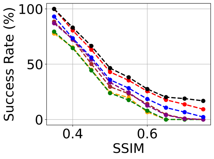
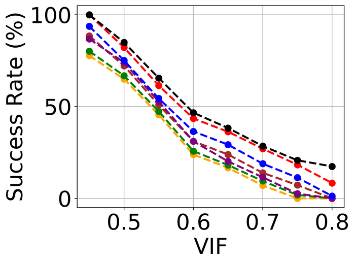
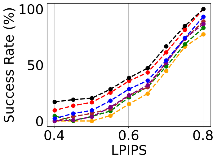
Evaluation metrics

Since we have the groundtruth clean images for both the synthetic and real-world data, we quantify and compare the performance of all selected BID methods using reference-based image quality assessment metrics. Besides the standard PSNR (peak signal-to-noise ratio) and SSIM (similarity structural index metric) metrics, we also take the information-theoretic VIF (visual information fidelity SheikhBovik2006Image ) and DL-based metric LPIPS (learned perceptual image patch similarity, zhang2018unreasonable ) that have shown good correlation with human perception of image quality. We report all four metrics in all our quantitative results below.

Model size and speed

For our method, the total number of parameters is about $2.3$ million, and on average, it takes about $10$ minutes (on an Nvidia V100 GPU) to reconstruct a sharp image of size $1000\times 1000$. SelfDeblur  gets a similar number of parameters and is slightly faster ($\sim 8$ minutes). In this paper, we prioritize quality over speed, and hence we do not perform a systematic benchmark of speed, especially with respect to data-driven methods, for which inference only takes a single forward pass. Our recent work LiEtAl2022Random addresses the speed issue of DIP; we leave the potential integration as future work.

Figure 20: Comparison of the performance of the $6$ selected single-instance BID methods on LEVIN11 with various levels of kernel-size overspecification. For PSNR, SSIM, and VIF, higher the better. For LPIPS, lower the better. The dashed lines indicate the performance baselines where the blurry image $𝐲$ and the groundtruth image $𝐱$ are directly compared.

Figure 21: Comparison of the performance of the $6$ selected single-instance BID methods on LAI16 with various levels of kernel-size overspecification. For PSNR, SSIM, and VIF, higher the better. For LPIPS, lower the better. The dashed lines indicate the performance baselines where the blurry image $𝐲$ and the groundtruth image $𝐱$ are directly compared.

4.2 Results on synthetic datasets

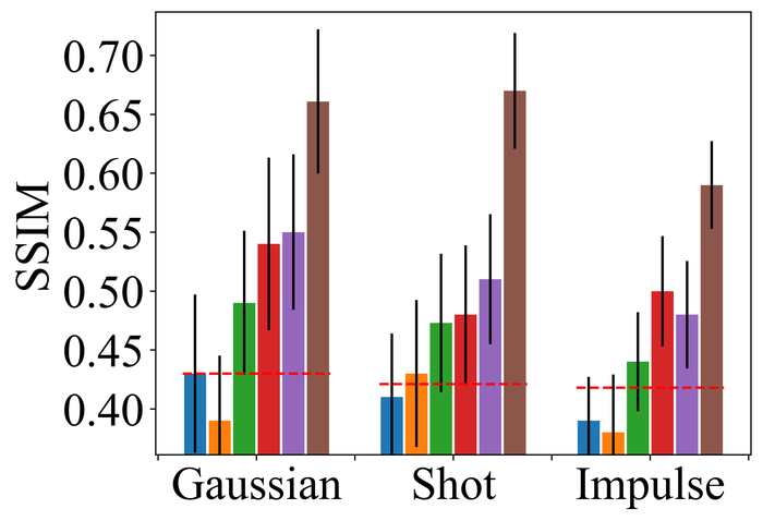
Among single-instance methods, we pick SunEtAl2013Edge (SUN13) that is among the top performing methods according to the 2016 survey paper LaiEtAl2016Comparative , and PanEtAl2016Blind (PAN16) that introduces the dark channel prior to BID and has been popular since 2016. We also select DongEtAl2017Blind (DONG17) which is a SOTA method that handles pixel corruptions, and SiYaoEtAl2019Understanding (SY19) among the first single-instance BID works addressing unknown kernel sizes. SelfDeblur  RenEtAl2020Neural inspires our method and hence is the main competitor. Together with our methods, all of the $6$ methods target the uniform setting in Eq. 1.

We strive to make the comparison fair while highlighting methods that require no heavy hyperparameter tuning—in practice, we never know the exact level of overspecification or type/level of noise. So we always use the same set of hyperparameters for each method. SUN13 and PAN16 are not designed to handle kernel-size overspecification and substantial noise; we directly use their default hyperparameters as it is unclear how to finetune them to optimize the performance in these novel scenarios. SY19 allows kernel-size overspecification and provides a set of hyperparameters for twice kernel-size overspecification. We follow their recommendation for twice overspecification, and search and select an optimal set of hyperparameters over a grid beyond twice overspecification. For DONG17 that handles substantial noise and pixel outliers, we use their default hyperparameter setting that is claimed to be general over different datasets. For SelfDeblur, we use their default setting, except that ${\lambda }_{𝐱}$ set as ${\lambda }_{𝐱}=1\mathrm{e}-5$ instead of their default ${\lambda }_{𝐱}=1\mathrm{e}-6$. This is because we observe that larger ${\lambda }_{𝐱}$ is needed to optimize the performance of SelfDeblur  as the noise level grows. For our method, we set ${\lambda }_{𝐱}=1\mathrm{e}-5$. All numbers that we report below are averages over images of the respective datasets.

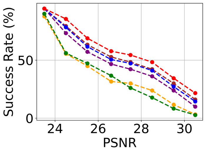
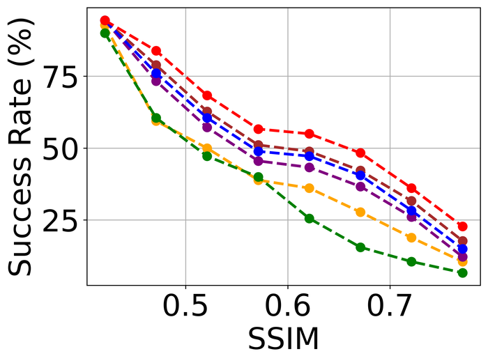
4.2.1 Kernel-size overspecification

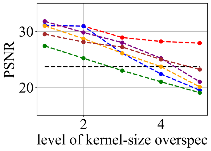
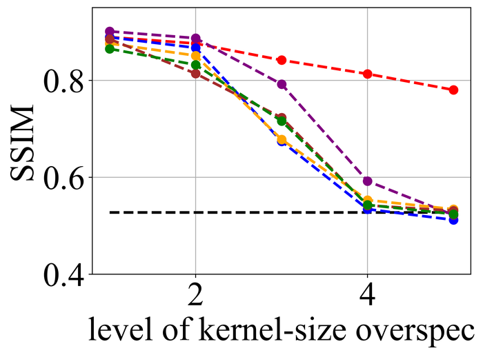
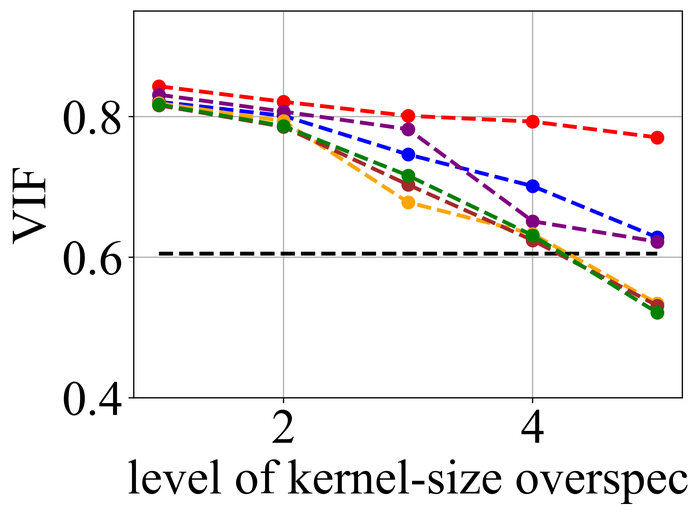
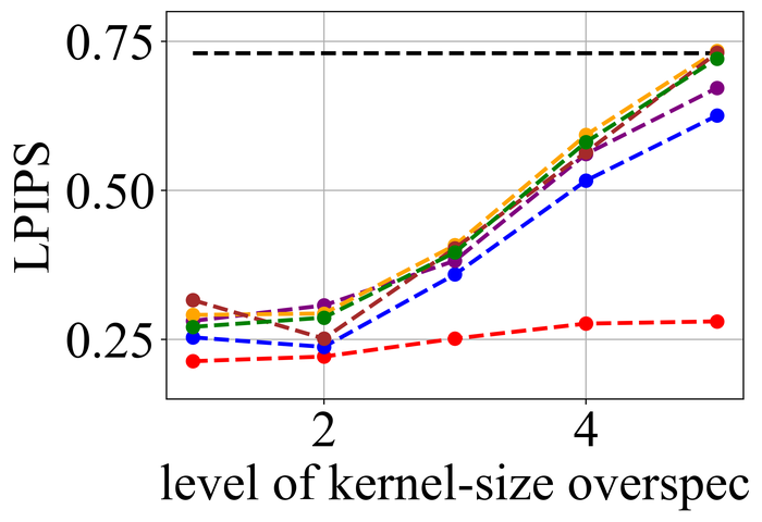
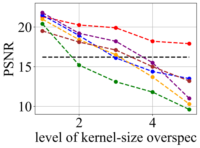
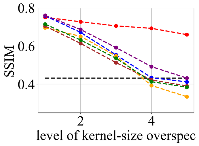
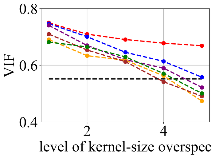
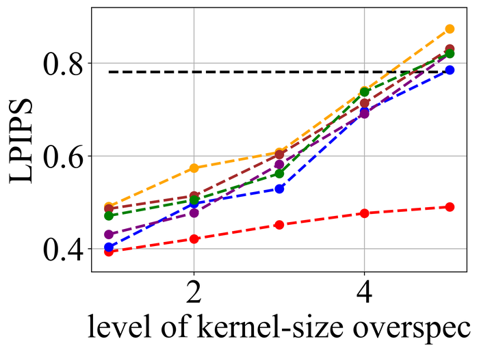
We first evaluate the stability of the selected methods under kernel-size overspecification. Since we know the true kernel size for each instance, we divide the overspecification into $5$ levels: level $1$ corresponds to the true kernel size, level $5$ corresponds to half of the image size in both width and height directions—which is the default over-specification level for our method, and levels $2$–$4$ are evenly distributed in between.

Figs. 20 and 21 summarize the results on LEVIN11 and LAI16, respectively. We observe that:

• When there is no kernel-size overspecification (i.e., level 1), SelfDeblur  PAN16, and our method are among the top three performing methods (sometimes tied with other methods) by all metrics. This confirms the effectiveness of double-DIP ideas for BID;

• As the overspecification level grows, the performance of all methods degrades, but our method is substantially more stable to such overspecification than other methods. In particular, for level-5 overspecification, while all of the other five methods become close or even worse than the baseline performance—where the blurry image $𝐲$ is directly taken to calculate the metrics, our method still performs strongly and shows considerable positive performance margins over the baseline;

• The performance of all methods becomes uniformly lower moving from LEVIN11 to LAI16. This is especially obviously on the pixel-based metrics PSNR and SSIM. We suspect there is mostly due to the larger kernel sizes in LAI16 ($27\times 27$ largest in LEVIN11 vs $31\times 31$ smallest in LEVIN11), which mess up large areas of pixels in each location;

• SY19, the only previous single-instance method that explicitly handles kernel-size overspecification, does not perform well—despite our best effort to search for an optimal set of hyperparameters. In their paper SiYaoEtAl2019Understanding , they have reported promising results with twice overspecification on LEVIN11, much less aggressive than our evaluation: for example, for $13\times 13$ kernels, they have tried $26\times 26$ overspecification, but here we experiment with $13\times 13$, $42\times 42$, $71\times 71$, $100\times 100$, and $128\times 128$. We suspect that the disappointing performance is due to the sensitivity of their method to hyperparameters across different overspecification levels.

Figure 22: Comparison of the performance of the $6$ selected single-instance BID methods on LAI16 with low-level additive noise: Gaussian ($\sigma =0.001$), shot ($\eta =80$), and impulse ($p=0.01$). For PSNR, SSIM, and VIF, higher the better. For LPIPS, lower the better. The dashes lines indicate the baseline performance where the blurry image $𝐲$ and the groundtruth image $𝐱$ are directly compared.

Figure 23: Comparison of the performance of the $6$ selected single-instance BID methods on LAI16 with high-level additive noise: Gaussian ($\sigma =0.05$), shot ($\eta =40$), and impulse ($p=0.05$). For PSNR, SSIM, and VIF, higher the better. For LPIPS, lower the better. The dashes lines indicate the baseline performance where the blurry image $𝐲$ and the groundtruth image $𝐱$ are directly compared.

Figure 24: Comparison of the performance of the $6$ selected single-instance BID methods on LAI16 with pixel saturation. For any fixed operation point of the evaluation metric (i.e., the horizontal axis), the success rate is defined as the fraction of images recovered at that quality or higher. For PSNR, SSIM, and VIF, higher the better. For LPIPS, lower the better.

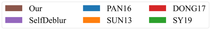
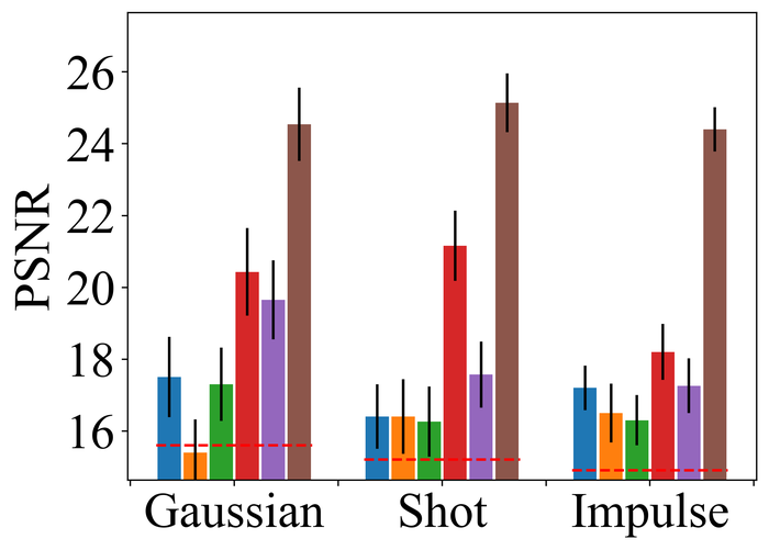
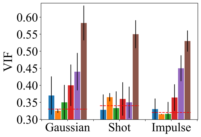
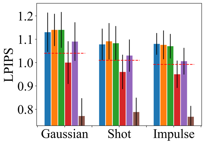
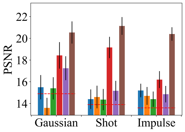
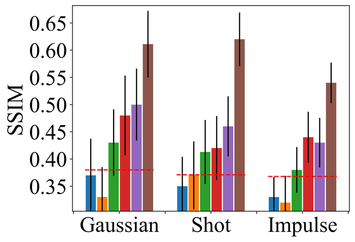
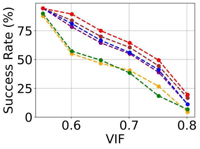
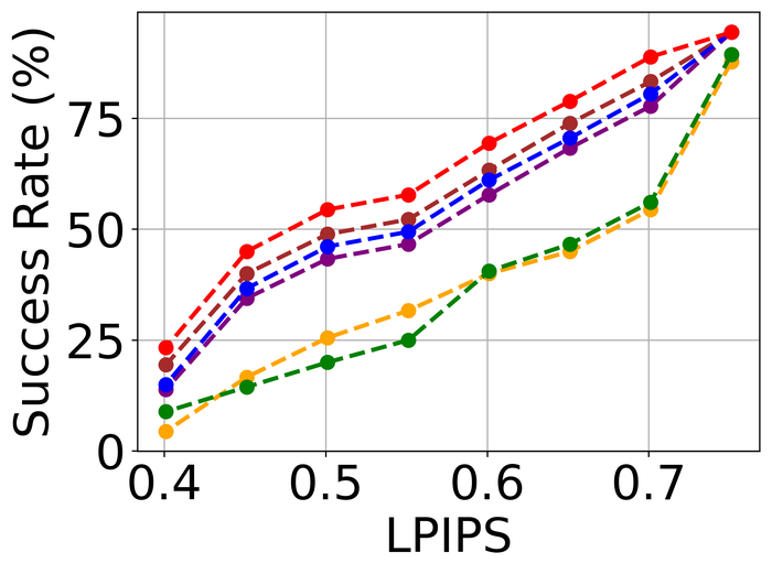
4.2.2 Substantial noise

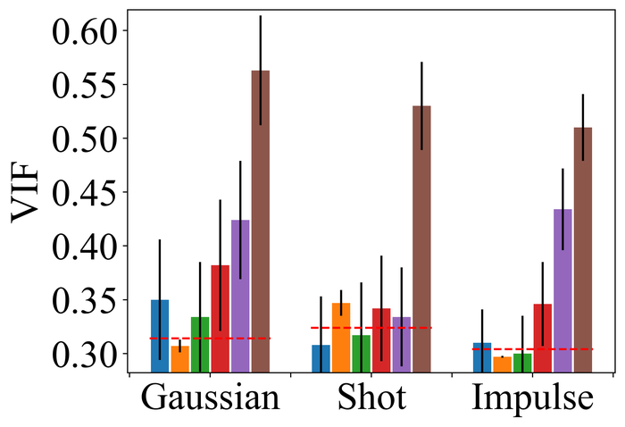
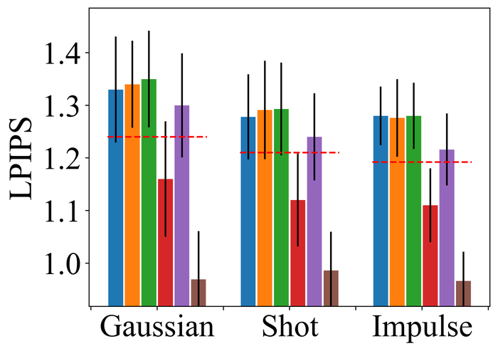
To evaluate the noise stability, we fix the kernel-size overspecification as half of the image size in both directions (i.e., the default for our method) for all methods, and focus on LAI16. We consider $4$ types of noise that have been considered in prior works:

• Gaussian noise: zero-mean additive Gaussian noise with standard deviation $\sigma =0.001$ and $\sigma =0.05$ for low and high noise levels, respectively;

• Impulse noise (i.e., salt-and-pepper noise): replacing each pixel with probability $p\in [0,1]$ into white ($1$) or black ($0$) pixel with half chance each. Low and high noise levels correspond to $p=0.005$ and $p=0.08$, respectively;

• Shot noise (i.e., pixel-wise independent Poisson noise): for each pixel $x\in [0,1]$, the noisy pixel is Poisson distributed with rate $\eta x$, where $\eta =90,25$ for low and high noise levels, respectively;

• Pixel saturation: each blurry RGB image $𝐲$ in LAI16 is first converted into HSV (i.e., hue-saturation-lightness) representation ${𝐲}_{\mathrm{HSV}}$ with values in $[0,1]$, and then the saturation channel is rescaled by a factor of $2$, shifted by a factor $0.1$, and then cropped into $[0,1]$. The resulting HSV representation is then converted back to RBG representation, with all values cropped back into $[0,1]$. We further add pixel-wise zero-mean Gaussian noise with standard deviation $\sigma =0.0001$.

Figs. 22 and 23 present the results on the first three types of noise, for the low- and high-level, respectively. As expected, all methods perform worse when moving from low- to high-level noise. DONG17, SelfDeblur, and our method are the top three performing methods by all metrics, for both low- and high-level noise. While SelfDeblur  is even worse than the trivial baseline (i.e., when no BID method is applied) by LPIPS, both DONG17 and ours always outperform the baseline—both use robust losses that are less sensitive to large errors compared to the standard MSE loss. Our method is the top performer and always win the second best, i.e., DONG17, by large margins by all metrics.

We observe similar performance trends of these methods in terms of handling pixel saturation, from Fig. 24: SelfDeblur, DONG17, and ours are the top three methods, with our method outperforming the other two by considerable margins. Based on these results, we conclude that using robust losses for BID is crucial to achieving robustness to practical noise.

Figure 25: Comparison of the performance of the $6$ selected single-instance BID methods on LAI16 with high-level noise only (no blur). DIP denotes a single-DIP model that does not account for blur at all, i.e., knowing the image is noise-only. The noise is randomly selected from Gaussian ($\sigma =0.1$), shot ($\eta =40$), and impulse ($p=0.08$) per image. For any fixed operation point of the evaluation metric (i.e., the horizontal axis), the success rate is defined as the fraction of images recovered at that quality or higher. For PSNR, SSIM, and VIF, higher the better. For LPIPS, lower the better.

Figure 26: Examples of estimated kernels of the $6$ selected single-instance BID methods on LAI16 with high-level noise only (no blur, same setting as in Fig. 25).

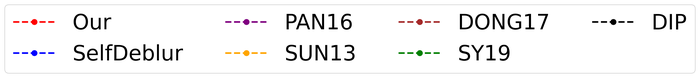
4.2.3 Model stability

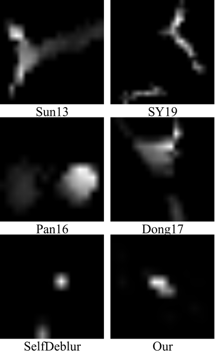
To evaluate model stability, we simulate noise-only images without blurs. For each image, we randomly pick one of the three types of high-level noise: Gaussian ($\sigma =0.1$), shot ($\eta =40$), and impulse ($p=0.08$), and apply it to produce the simulated noisy image. Note that the individual noise levels are considerably higher than those used in Fig. 23. The reason is that we hope to stretch the difficulty level of the test: intuitively, an ideal BID method should tolerate more noise on a noise-only input than on a blurry-and-noisy input. As far as we are aware, this is the first evaluation of SOTA BID methods in terms of model stability.

The results are presented in Fig. 25. There, DIP denotes the single-DIP method that directly models the noise only, i.e., by considering

$\underset{{\theta }_{𝐱}}{\min }{\mathrm{\ell }}_{\mathrm{Huber}}(𝐲,G_{{\theta }_{𝐱}}({𝐳}_{𝐱}))+{\lambda }_{𝐱}{\displaystyle \frac{{\Vert {\nabla }_{𝐱}{G}_{{\theta }_{𝐱}}({𝐳}_{𝐱})\Vert }_1}{{\Vert {\nabla }_{𝐱}{G}_{{\theta }_{𝐱}}({𝐳}_{𝐱})\Vert }_2}}.$

We use exactly the same architecture for $G_{{\theta }_{𝐱}}$ and the same ${\lambda }_{𝐱}$ as used in our method. Since this method incorporates the knowledge that the image has no blur, it is not surprising it performs the best. Immediately after, it is evident that SelfDeblur  and ours are the clear winners by all metrics, and ours leads SelfDeblur  by visible margins. Moreover, the performance of our method approaches that of DIP, suggesting strong model stability of our method. Unfortunately, although DONG17 can tolerate substantial noise together with blur, it does not work well when there is no blur. In fact, the estimated kernels of the four non-Double-DIP methods (i.e., SUN13, SY19, PAN16, DONG17) are far from the delta function—which is the true kernel in this case, as shown in Fig. 26. In contrast, SelfDeblur  and our method recover kernels that resemble the delta function. Besides the common sparse gradient prior on the image used by all methods, SelfDeblur  and our method also enforce the DIP on the image. We suspect that their superior model stability can be attributed to the simultaneous use of the two priors instead of only one. We reiterate that we do not finetune the hyperparameters of any method moving from the previous blurry-and-noisy test to the current noise-only test: finetuning may improve certain methods, but is deemed impractical as we often do not have such model knowledge about real data.

Figure 27: Detection performance of WMV-ES on LAI16. Each plot corresponds to one metric we use, and collects the histogram of the ES-Gap (gap between the true peak performance and the detected performance) and the Base-Gap (gap between the true peak performance and the performance at the last iteration).

4.2.4 Early stopping

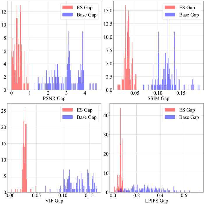
As we discussed in Section 3.1.5, ES is necessary and practical for preventing overfitting when there is substantial noise. Here, we test the WMV-ES method WangEtAl2021Early that we use by default, on LAI16 with low- and high-level Gaussian noise (as defined in Section 4.2.2). Fig. 27 presents the histograms of ES gap (between the peak performance and the detected performance by the ES method) and the Base gap (between the peak performance and the final performance with overfitting), using all of the four metrics. It is clear that ES is crucial to saving the performance: without ES, the eventual overfitting of double-DIP to noise ruins the recovery, e.g., reducing the PSNR by $3$ points or more for a large portion of the images; with the automatic ES method WMV-ES, we are only slightly off the peak performance—just to be sure, without knowing the groundtruth in practice, we cannot directly stop the algorithm right at the peak performance point. The success of WMV-ES is evident from the clear separation of the histograms between ES Gap and Base Gap, by all of the metrics.

4.3 Results on real-world datasets

4.3.1 Competing methods and data preparation

It is clear by far that the $5$ competing methods that we worked with above are not good choices for real-world BID, due to their sensitivity to kernel-size overspecification and substantial noise. On the other hand, most of the recent SOTA BID methods are data-driven in nature: although they may not be generalizable as limited by the training data, they are attractive as most recent variants directly predict sharp images from blurry images and hence bypass the problems caused by unknown kernel size and even inaccurate blur modeling KohEtAl2021Single . Hence, in this section, we stretch our method, as well as SelfDeblur, by comparing them with $3$ SOTA data-driven methods on the SOTA NTIRE2020 and RealBlur BID datasets.

Scale-recurrent network (SRN) tao2018scale and GAN-based DeblurGAN-v2 kupyn2019deblurgan are BID models trained on paired blurry-sharp image pairs. The prediction models for both take inspiration from the coarse-to-fine multiscale ideas in traditional BID. In addition, DeblurGAN-v2 employs GAN-based discriminators as regularizers to improve the deblurring quality. ZHANG20 zhang2020deblurring stresses the practical difficulty in obtaining blurry-sharp training pairs (echoing the discussion of similar difficulty in KohEtAl2021Single ; ZhangEtAl2022Deep ), and derives a pipeline to learn the blurring and deblurring processes from unpaired blurry and sharp images. For the comparison below, we directly take the pretrained models of the $3$ methods . We note that both SRN and DeblurGAN-v2 use the GoPro dataset NahEtAl2017Deep as part of their training sets, and ZHANG20 builds their own blurry training set RWBI zhang2020deblurring . To the best of our knowledge, NTIRE2020 and RealBlur have no overlap with GoPro and RWBI. So we believe our evaluation set makes a good test for real-world generalizability of the $3$ selected methods.

Figure 28: Illustration of image selection from NTIRE2020 (top) and RealBlur (bottom), respectively. For images from the same dynamic/static scene, we always select visually the most blurry image (highlighted by red bounding boxes).

Figure 29: Comparison of deblurring results on a bright scene with high depth contrast

Figure 30: Comparison of deblurring results on a dark scene with high depth contrast

Figure 31: Comparison of deblurring results on a bright scene with low depth contrast

Figure 32: Comparison of deblurring results on a dark scene with low depth contrast

Figure 33: Comparison of deblurring results on a scene with high depth contrast and high brightness contrast

Figure 34: Failure case: Comparison of deblurring results on a scene with high depth contrast and high brightness contrast

Table 2: Quantitative comparison of deblurring results on the $125$ selected real-world images. For PSNR, SSIM, and VIF, higher the better. For LPIPS, lower the better. S1–S5 represent the $5$ scenarios described in Section 4.3.1. We report in the form of “mean (standard deviation)” (over the $125$ images) for each method/metric combination. For each line, the first and second best numbers (according to the means) are marked in RED and GREEN, respectively.

		SRN	DeblurGAN-v2	ZHANG20	SelfDeblur	Ours
S1	PSNR	30.1 (1.159)	31.0 (1.149)	25.2 (1.188)	28.2 (1.198)	30.8 (1.168)
	SSIM	0.871 (0.0679)	0.883 (0.0609)	0.793 (0.0724)	0.832 (0.0734)	0.873(0.0618)
	VIF	0.784 (0.0686)	0.801 (0.0647)	0.705 (0.0705)	0.725 (0.0727)	0.796 (0.0651)
	LPIPS	0.972 (0.0966)	0.827 (0.08869)	1.025 (0.104)	0.987 (0.101)	0.821 (0.0879)
S2	PSNR	27.1 (1.256)	27.4 (1.352)	23.4 (1.449)	25.9 (1.471)	28.7 (1.236)
	SSIM	0.851 (0.0744)	0.859 (0.0695)	0.789 (0.0753)	0.821 (0.0758)	0.870 (0.0681)
	VIF	0.772 (0.0778)	0.783 (0.0758)	0.699 (0.0787)	0.713 (0.0777)	0.781 (0.0767)
	LPIPS	1.021 (0.116)	0.901 (0.0985)	1.076 (0.108)	1.001 (0.111)	0.811 (0.0947)
S3	PSNR	28.3 (1.197)	28.7 (1.139)	25.2 (1.236)	26.2 (1.227)	29.4 (1.144)
	SSIM	0.866 (0.0647)	0.867 (0.0608)	0.803 (0.0658)	0.827 (0.0637)	0.872 (0.0589)
	VIF	0.761 (0.0772)	0.787 (0.0727)	0.701 (0.0766)	0.731 (0.0776)	0.780 (0.0679)
	LPIPS	1.008 (0.0985)	0.869 (0.0936)	1.076 (0.107)	0.985 (0.110)	0.839 (0.0911)
S4	PSNR	26.7 (1.014)	27.1 (0.985)	23.3 (1.043)	25.8 (1.055)	28.5 (0.947)
	SSIM	0.849 (0.0542)	0.851 (0.0498)	0.780 (0.0567)	0.812 (0.0578)	0.861 (0.0481)
	VIF	0.756 (0.0621)	0.767 (0.0592)	0.687 (0.0663)	0.721 (0.0674)	0.776 (0.0574)
	LPIPS	1.015 (0.0941)	0.925 (0.0862)	1.050 (0.0927)	0.996 (0.0674)	0.893 (0.0848)
S5	PSNR	28.6 (1.352)	28.7 (1.314)	24.7 (1.410)	26.4 (1.400)	29.2 (1.284)
	SSIM	0.846 (0.0754)	0.855 (0.0694)	0.781 (0.0762)	0.818 (0.0771)	0.867 (0.0674)
	VIF	0.756 (0.0756)	0.771 (0.0754)	0.692 (0.0784)	0.710 (0.0793)	0.776 (0.0761)
	LPIPS	1.012 (0.1093)	0.874 (0.1085)	1.065 (0.1141)	0.992 (0.1149)	0.856 (0.0945)

As alluded to above, both NTIRE2020 and RealBlur have their own strengths and limitations: images in NTIRE2020 may contain multiple motions, but are captured in well-lit environments; RealBlur covers many dark scenes, but the scenes are static and relative motions are caused by camera shakes only. In preliminary tests, we find the $3$ selected data-driven methods perform vastly differently across images, even within the same dataset. The dictating factors seem to include contrast of scene depth, contrast of brightness, and the combination thereof: different scene depths likely correspond to different relative motions, especially in the data of NTIRE2020, as well as different levels of defocus blur, while relative to the bright areas, dark areas tend to be less attended to by typical losses. Hence, we choose both NTIRE2020 and RealBlur: the former contains a good portion of images with good depth contrast and multiple moving objects, and the latter provides samples with good brightness and depth contrast.

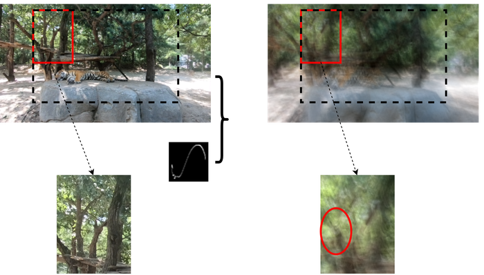
We select $125$ representative, visually challenging images from the two datasets: for NTIRE 2020, we pick the most blurry frame from each folder that contains a sequence of consecutive frames; similarly, for RealBlur, we pick the most blurry one from images about the same scene. Fig. 28 gives a couple of examples to illustrate our selection. The $125$ images are classified into $5$ scenarios—$25$ images each: (S1) bright scene with high depth contrast (see an example in Fig. 29); (S2) dark scene with high depth contrast (see an example in Fig. 30); (S3) bright scene with low depth contrast (see an example in Fig. 31); (S4) dark scene with low depth contrast (see an example in Fig. 32); (S5) scene with high depth contrast and high brightness contrast (see an example in Fig. 33). NTIRE2020 only includes bright scenes, and we pick $35$ images from it: $25$ for S1, and $10$ for S3. Then, from RealBlur, we choose $15$ images to complete S3, and $25$ images for each of S2, S4, and S5, respectively. For reproducibility of our results, the IDs of the selected images can be found in our Github repository: https://github.com/sun-umn/Blind-Image-Deblurring.

4.3.2 Qualitative and quantitative results

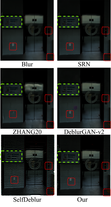
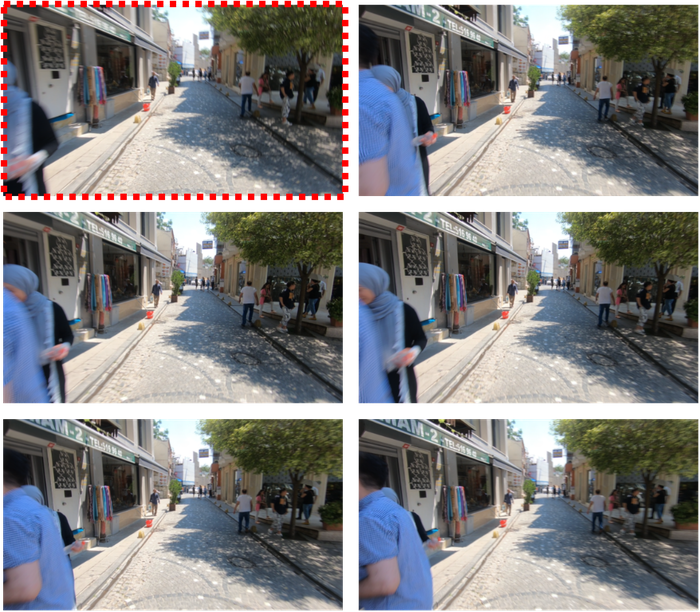
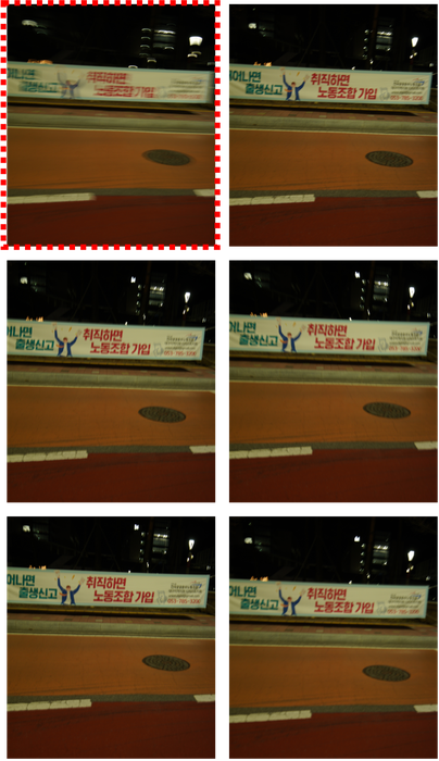
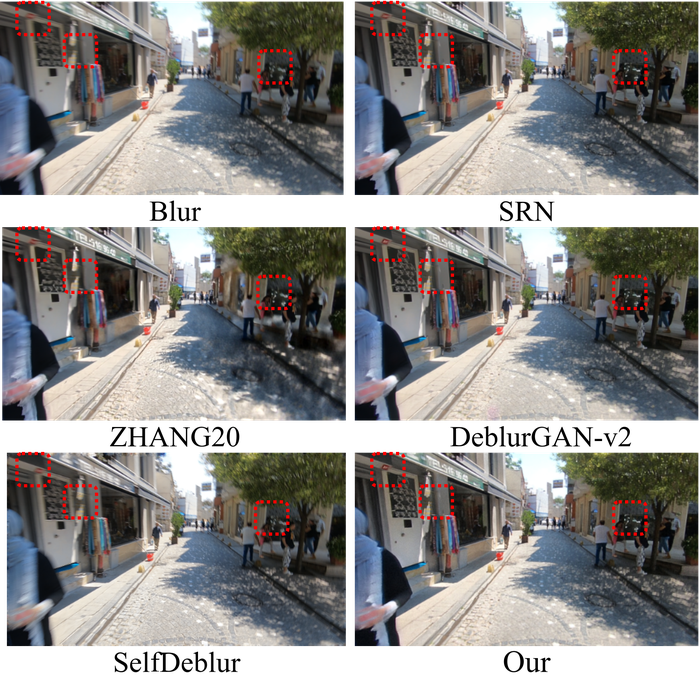
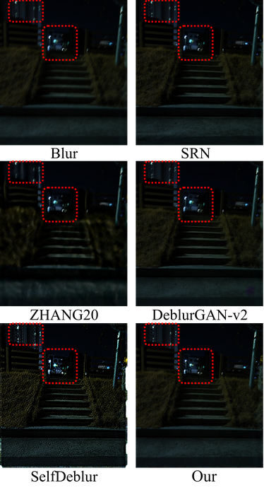
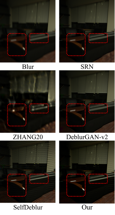
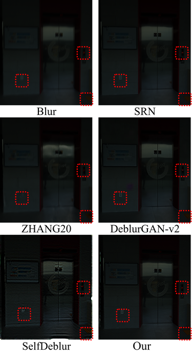
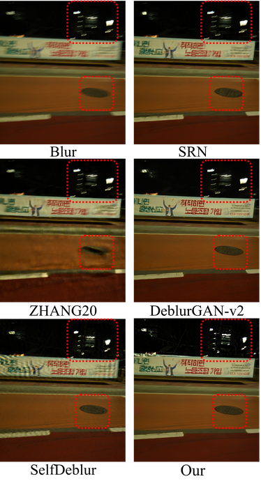
Figs. 29, 33, 30, 31 and 32 present $5$ blurry images (Fig. 30 and Fig. 32 are too dark to reveal enough details; we apply histogram equalization to enhance the contrast and include them in Section 6.2), each representing one of the $5$ scenarios, and the recovery results from SRN, ZHANG20, DeblurGAN-v2, SelfDeblur, and our method. Table 2 summarizes the quantitative results over the $125$ selected images using the metrics: PSNR, SSIM, VIF, and LPIPS.

Our method wins in most cases, followed by GAN-based DeblurGAN-v2. In fact, they are the top two in all cases. DeblurGAN-v2 leads our method on S1 by all metrics except for LPIPS, and on S2 and S3 only by VIF. This is likely because S1 is sampled entirely from NTIRE2020 that consists of bright scenes only, similar to the GoPro dataset that DeblurGAN-v2 is trained on; only $10$ out of $25$ images from S3 are from NTIRE2020. On S2, S4, and S5 where each image consists of part of dark scenes, our method is a clear winner. This can be explained by the emphasis of the RealBlur dataset on dark scenes that have different distributions than GoPro that only includes bright scenes. It is remarkable that our method, a non-data-driven method, can performs on par with SOTA data-driven methods on similar data the latter are trained on, and can perform consistently better on novel data. The performance discrepancy of DeblurGAN-v2 on different scenarios again underscores how data-driven methods can be limited by the training data, although overall DeblurGAN-v2 indeed shows reasonable generalizability to the novel dataset RealDeblur.

ZHANG20, the worst performer in our evaluation, is trained on the Real-World Blurry Image (RWBI) dataset collected by the same group of authors zhang2020deblurring . Visual inspection into RWBI suggests the blurry scenes are mostly similar to those of GoPro: bright scenes, none or few moving objects, substantial camera motions. So it is no surprise that the original paper zhang2020deblurring reports encouraging generalization performance of their pretrained model on GoPro. By contrast, NTIRE2020 images are mostly taken about much more complex scenes with multiple moving objects plus synthetic camera motions, and RealBlur emphasizes dark scenes. The significant distribution shift explains the relatively poor performance of their pretrained model in our evaluation, as seen from Table 2 and the visual results in Figs. 29, 33, 30, 31 and 32, and underscores again the generalizability issue around data-driven methods. Note that SRN is originally trained and tested on GoPro, and hence is subject to similar distribution shift and performance drop. But, SRN is trained on sharp-blurry image pairs, whereas ZHANG20 on unpaired sharp and blurry images and so the input knowledge is much weaker and the learning task is more challenging, explaining why SRN is stronger in performance and comes close to DeblurGAN-v2. SelfDeblur that our method builds on obviously lags behind. From Figs. 33, 30, 31 and 32, we can see obvious texture artifacts in the image contents that SelfDeblur recovers, as well as boundary noise (especially in Figs. 30 and 32) due to the improper cropping used by SelfDeblur (discussed in Section 3.1.2).

4.4 Failure cases and limitations

We highlight three major factors that can cause failures: 1) substantial depth contrast that makes the uniform model less accurate; 2) kernel size overspecification that makes kernel estimation challenging; 3) inaccurate localization of the estimated $\widehat{𝐱}$ that induces boundary noise. Below, we include a couple of failure examples and brief explanations resorting to these factors.

In Fig. 31, we can see strip artifacts in the window region from both SelfDeblur  and our method. We suspect that the strips are due to combined effects of 1) and 2) above. This is experimentally confirmed in Fig. 35 below: as we reduce the kernel-size overspecification, the strips are gone, but the recovered foreground floor region also becomes over-smooth and misses details.

Figure 35: Effect of reducing the kernel-size overspecification in our method for Fig. 31

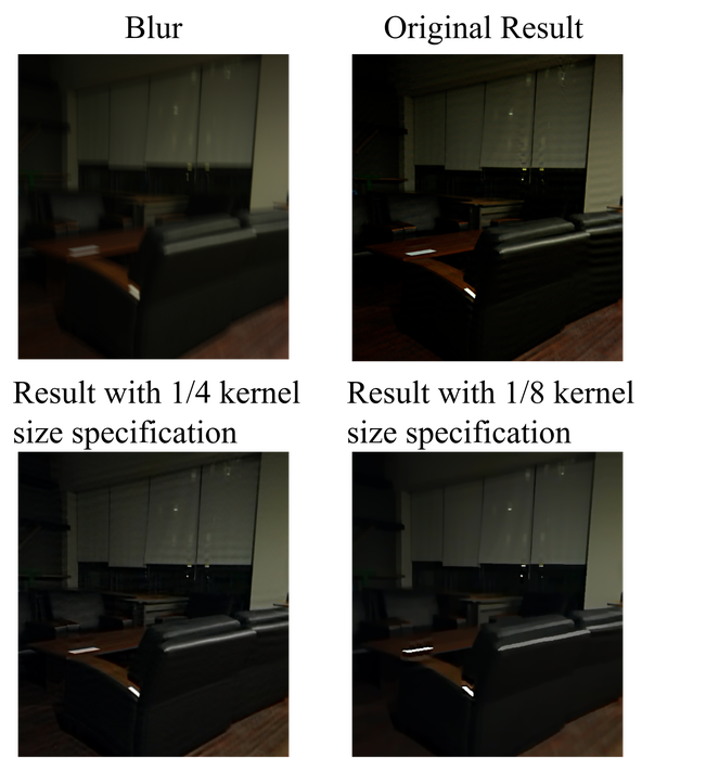
Fig. 34 shows a difficult case that fails all methods, including ours. The failure is likely due to: 1) huge depth contrast that violates the uniform model leading to both varying defocus and motion blurs. As is evident, DeblurGAN-v2, SelfDeblur, and ours are among the best performers, but they can only recover reasonable details in the foreground and not the far-away lights; 2) localization of the estimated $\widehat{𝐱}$ specific to SelfDeblurand ours. We can see clear spurious light spots near the top-right corners of the reconstructions by both methods.

Table 3: Sensitivity analysis of our method with respect to key hyperparameters. LR: learning rate; ${\lambda }_{𝐱}$: regularization parameter for the ${\mathrm{\ell }}_1/{\mathrm{\ell }}_2$ regularizer. For PSNR, SSIM, and VIF, higher the better. For LPIPS, lower the better. Default parameters and their results are highlighted in boldface.

LR	$5\mathrm{e}-3$	$\mathrm{𝟏}\mathrm{e}-\mathrm{𝟑}$	$5\mathrm{e}-4$	$1\mathrm{e}-4$	$5\mathrm{e}-4$	$1\mathrm{e}-5$
PSNR	26.9	29.3	28.7	27.9	27.8	27.8
SSIM	0.774	0.869	0.828	0.813	0.793	0.790
VIF	0.691	0.781	0.735	0.725	0.716	0.709
LPIPS	0.972	0.844	0.875	0.901	0.921	0.927

${\lambda }_{𝐱}$	$5\mathrm{e}-4$	$1\mathrm{e}-4$	$\mathrm{𝟏}\mathrm{e}-\mathrm{𝟓}$	$5\mathrm{e}-5$	$5\mathrm{e}-6$	$1\mathrm{e}-6$
PSNR	26.3	27.7	29.3	28.3	27.7	27.2
SSIM	0.763	0.813	0.869	0.822	0.803	0.793
VIF	0.681	0.725	0.781	0.745	0.716	0.703
LPIPS	1.021	0.902	0.844	0.887	0.925	0.931

4.5 Ablation study

Learning rates (for ${\theta }_{𝐤}$ and ${\theta }_{𝐱}$, respectively) and the regularization parameter ${\lambda }_{𝐱}$ are the two crucial groups of hyperparameters for our method. Hence, in this ablation study, we focus on these two factors, and perform experiments on the real-world images used in Section 4.3. We lock all other hyperparameters to our default setting.

We lock the LR ratio for ${\theta }_{𝐱}$ and ${\theta }_{𝐤}$ to be $100:1$, and hence only specify the LR for ${\theta }_{𝐱}$ when presenting the results. Table 3 (top) includes the $6$ groups of LRs we have tried, and the resulting performance. When the LR is higher than $1\mathrm{e}-2$, the training fails to converge properly. When we decrease the LR below $1\mathrm{e}-2$, the perform degrades gradually. This is due to that the small LRs entail more iterations to converge, whereas we cap the maximum number of iterations for efficiency.

The regularization parameter ${\lambda }_{𝐱}$ controls the trade-off between the data fitting and the enforcement of the sparse gradient prior (see Section 3.2). We also vary ${\lambda }_{𝐱}$ across $6$ levels, covering the $1\mathrm{e}-4\sim 1\mathrm{e}-6$ range, and summarize the results in Table 3 (bottom). We note that we take the mean of Huber loss over all pixels for the data fitting term, but the ${\mathrm{\ell }}_1/{\mathrm{\ell }}_2$ regularizer scales roughly as $O(\sqrt{\mathrm{\#}\text{pixels}})$ which is around $1\mathrm{e}3$ for real-world color images. So the base ${\lambda }_{𝐱}$ should be $1\mathrm{e}-3$ to cancel out the dimension factor. Our optimal regularization level $1\mathrm{e}-5$ is hence $1\mathrm{e}-2$ in the effective level. Our method is stable when ${\lambda }_{𝐱}$ is on the $1\mathrm{e}-5$ level, and degrades considerably for levels above or below $1\mathrm{e}-5$.

5 Discussion

In this paper, we have proposed crucial modifications to the recent SelfDeblur method RenEtAl2020Neural for BID, and these modifications help successfully tackle the pressing practicality issues around BID: unknown kernel size, substantial noise, and model stability. Systematic evaluation of our method on both synthetic and real-world data confirms the effectiveness of our method. Remarkably, although our method only assumes the simple uniform blur model (i.e., Eq. 1), it performs comparably or superior to SOTA data-driven methods on real-world blurry images—these data-driven methods do not assume explicit forward models and hence are presumably much less constrained, but are limited by the expressiveness of their respective training data that are tricky to collect.

There are multiple directions to extend and generalize the current work. First, the performance of our method on real-world data likely can be further improved if we model non-uniform blur; our forthcoming work ZhuangEtAl2023NBID does exactly this. Second, similar to traditional BID methods that are based on iterative optimization, our method is slow compared to the emerging data-driven methods. One can possibly address this by designing compact DIP models that allow efficient optimization (see, e.g., LiEtAl2022Random ), and also by initializing the current DIP-based method using SOTA data-driven methods. Third, in principle our method can be readily extended to blind video deblurring, although it seems that one needs to address the increased modeling gap and computational cost. Fourth, the principle of modeling the object of interest by multiple DIP models or variants seems general for solving other inverse problems (see, e.g., our recent application of this to obtain breakthrough results in Fourier phase retrieval YangEtAl2022Application ; ZhuangEtAl2022Practical ).

Data availability statements

Part of the code and datasets used during the current study, necessary to interpret, replicate and build upon the findings reported in the article, are available in the Github repository https://github.com/sun-umn/Blind-Image-Deblurring

6 Appendix

6.1 List of common acronyms

Table 4: List of acronyms (in alphabetic order)

BID	blind image deblurring
BD	blind deconvolution
DIP	deep image prior
DL	deep learning
DNN	deep neural network
ES	early stopping
LPIPS	learned perceptual image patch similarity
LR	learning rate
MAP	maximum a posterior
MLP	multi-layer perceptron
MSE	mean squared error
PSNR	peak signal-to-noise ratio
SIREN	sinusoidal representation networks
SOTA	state-of-the-art
SSBD	short-and-sparse blind deconvolution
SSIM	structural similarity index measure
TV	total-variation
VAR	variance
VIF	visual information fidelity
VIP	visual inverse problem
WMV-ES	windowed-moving-variance-based ES

6.2 Contrast-enhanced version of Figs. 30 and 32

To reveal more details for images in Figs. 30 and 32 that are about extremely dark scenes, we perform histogram equalization to enhance the contrast and display the results as follows.

Figure 36: Contrast-enhanced version of Fig. 30 after histogram equalization.

Figure 37: Contrast-enhanced version of Fig. 32 after histogram equalization.

References

- (1) Ahmed, A., Recht, B., Romberg, J.: Blind deconvolution using convex programming. IEEE Transactions on Information Theory 60(3), 1711–1732 (2014). DOI 10.1109/tit.2013.2294644
- (2) Aljadaany, R., Pal, D.K., Savvides, M.: Douglas-rachford networks: Learning both the image prior and data fidelity terms for blind image deconvolution. In: 2019 IEEE/CVF Conference on Computer Vision and Pattern Recognition (CVPR). IEEE (2019). DOI 10.1109/cvpr.2019.01048
- (3) Asim, M., Shamshad, F., Ahmed, A.: Blind image deconvolution using deep generative priors. IEEE Transactions on Computational Imaging 6, 1493–1506 (2020). DOI 10.1109/tci.2020.3032671
- (4) Benichoux, A., Vincent, E., Gribonval, R.: A fundamental pitfall in blind deconvolution with sparse and shift-invariant priors. In: IEEE International Conference on Acoustics, Speech and Signal Processing. IEEE (2013). DOI 10.1109/icassp.2013.6638838
- (5) Bostan, E., Heckel, R., Chen, M., Kellman, M., Waller, L.: Deep phase decoder: self-calibrating phase microscopy with an untrained deep neural network. Optica 7(6), 559–562 (2020)
- (6) Cabrelli, C.A.: Minimum entropy deconvolution and simplicity: A noniterative algorithm. Geophysics 50(3), 394–413 (1985). DOI 10.1190/1.1441919
- (7) Chan, T., Wong, C.K.: Total variation blind deconvolution. IEEE Transactions on Image Processing 7(3), 370–375 (1998). DOI 10.1109/83.661187
- (8) Chen, L., Fang, F., Wang, T., Zhang, G.: Blind image deblurring with local maximum gradient prior. In: IEEE Conference on computer vision and pattern recognition (CVPR). IEEE (2019). DOI 10.1109/cvpr.2019.00184
- (9) Chen, L., Fang, F., Zhang, J., Liu, J., Zhang, G.: OID: Outlier identifying and discarding in blind image deblurring. In: European Conference on Computer Vision (ECCV), pp. 598–613. Springer International Publishing (2020). DOI 10.1007/978-3-030-58595-2˙36
- (10) Chen, L., Zhang, J., Lin, S., Fang, F., Ren, J.S.: Blind deblurring for saturated images. In: IEEE Conference on computer vision and pattern recognition (CVPR). IEEE (2021). DOI 10.1109/cvpr46437.2021.00624
- (11) Cheung, S.C., Shin, J.Y., Lau, Y., Chen, Z., Sun, J., Zhang, Y., Müller, M.A., Eremin, I.M., Wright, J.N., Pasupathy, A.N.: Dictionary learning in fourier-transform scanning tunneling spectroscopy. Nature Communications 11(1) (2020). DOI 10.1038/s41467-020-14633-1
- (12) Chi, Y.: Guaranteed blind sparse spikes deconvolution via lifting and convex optimization. IEEE Journal of Selected Topics in Signal Processing 10(4), 782–794 (2016). DOI 10.1109/jstsp.2016.2543462
- (13) Cho, S., Lee, S.: Fast motion deblurring. In: ACM Trans. Graph. ACM Press (2009). DOI 10.1145/1661412.1618491
- (14) Cho, S., Lee, S.: Convergence analysis of MAP based blur kernel estimation. In: IEEE International conference on computer vision (ICCV). IEEE (2017). DOI 10.1109/iccv.2017.515
- (15) Choudhary, S., Mitra, U.: Sparse blind deconvolution: What cannot be done. In: IEEE International Symposium on Information Theory. IEEE (2014). DOI 10.1109/isit.2014.6875385
- (16) Choudhary, S., Mitra, U.: On the properties of the rank-two null space of nonsparse and canonical-sparse blind deconvolution. IEEE Transactions on Signal Processing 66(14), 3696–3709 (2018). DOI 10.1109/tsp.2018.2815014
- (17) Darestani, M.Z., Heckel, R.: Accelerated MRI with un-trained neural networks. IEEE Transactions on Computational Imaging 7, 724–733 (2021). DOI 10.1109/tci.2021.3097596
- (18) Ding, Z., Luo, Z.Q.: A fast linear programming algorithm for blind equalization. IEEE Transactions on Communications 48(9), 1432–1436 (2000). DOI 10.1109/26.870004
- (19) Dong, J., Pan, J., Su, Z., Yang, M.H.: Blind image deblurring with outlier handling. In: IEEE International conference on computer vision (ICCV). IEEE (2017). DOI 10.1109/iccv.2017.271
- (20) Donoho, D.: ON minimum entropy deconvolution. In: Applied Time Series Analysis II, pp. 565–608. Elsevier (1981). DOI 10.1016/b978-0-12-256420-8.50024-1
- (21) Ekanadham, C., Tranchina, D., Simoncelli, E.: A blind sparse deconvolution method for neural spike identification. In: Advances in Neural Information Processing Systems (2011)
- (22) Fang, L., Liu, H., Wu, F., Sun, X., Li, H.: Separable kernel for image deblurring. In: IEEE Conference on computer vision and pattern recognition (CVPR). IEEE (2014). DOI 10.1109/cvpr.2014.369
- (23) Gandelsman, Y., Shocher, A., Irani, M.: “double-DIP”: Unsupervised image decomposition via coupled deep-image-priors. In: IEEE Conference on computer vision and pattern recognition (CVPR). IEEE (2019). DOI 10.1109/cvpr.2019.01128
- (24) Gong, D., Tan, M., Zhang, Y., van den Hengel, A., Shi, Q.: Self-paced kernel estimation for robust blind image deblurring. In: IEEE International conference on computer vision (ICCV). IEEE (2017). DOI 10.1109/iccv.2017.184
- (25) Gong, D., Tan, M., Zhang, Y., Hengel, A.V.D., Shi, Q.: Blind image deconvolution by automatic gradient activation. In: IEEE Conference on computer vision and pattern recognition (CVPR). IEEE (2016). DOI 10.1109/cvpr.2016.202
- (26) Heckel, R., Hand, P.: Deep decoder: Concise image representations from untrained non-convolutional networks. In: International Conference on Learning Representations (2019)
- (27) Heckel, R., Soltanolkotabi, M.: Denoising and regularization via exploiting the structural bias of convolutional generators. arXiv preprint arXiv:1910.14634 (2019)
- (28) Heckel, R., Soltanolkotabi, M.: Compressive sensing with un-trained neural networks: Gradient descent finds the smoothest approximation. arXiv:2005.03991 (2020)
- (29) Hendrycks, D., Dietterich, T.: Benchmarking neural network robustness to common corruptions and perturbations. In: International Conference on Learning Representations (2019). URL https://openreview.net/forum?id=HJz6tiCqYm
- (30) Huber, P.J.: Robust estimation of a location parameter. The Annals of Mathematical Statistics 35(1), 73–101 (1964). DOI 10.1214/aoms/1177703732
- (31) Hurley, N., Rickard, S.: Comparing measures of sparsity. IEEE Transactions on Information Theory 55(10), 4723–4741 (2009). DOI 10.1109/tit.2009.2027527
- (32) Jin, M., Roth, S., Favaro, P.: Normalized blind deconvolution. In: European Conference on Computer Vision (ECCV), pp. 694–711. Springer International Publishing (2018). DOI 10.1007/978-3-030-01234-2˙41
- (33) Joshi, N., Szeliski, R., Kriegman, D.J.: PSF estimation using sharp edge prediction. In: IEEE Conference on computer vision and pattern recognition (CVPR). IEEE (2008). DOI 10.1109/cvpr.2008.4587834
- (34) Joshi, N., Zitnick, C.L., Szeliski, R., Kriegman, D.J.: Image deblurring and denoising using color priors. In: IEEE Conference on computer vision and pattern recognition (CVPR). IEEE (2009). DOI 10.1109/cvpr.2009.5206802
- (35) Kech, M., Krahmer, F.: Optimal injectivity conditions for bilinear inverse problems with applications to identifiability of deconvolution problems. SIAM Journal on Applied Algebra and Geometry 1(1), 20–37 (2017). DOI 10.1137/16m1067469
- (36) Koh, J., Lee, J., Yoon, S.: Single-image deblurring with neural networks: A comparative survey. Computer Vision and Image Understanding 203, 103134 (2021). DOI 10.1016/j.cviu.2020.103134
- (37) Komodakis, N., Paragios, N.: MRF-based blind image deconvolution. In: Asian Conference on Computer Vision (ACCV), pp. 361–374. Springer Berlin Heidelberg (2013). DOI 10.1007/978-3-642-37431-9˙28
- (38) Krishnan, D., Fergus, R.: Fast image deconvolution using hyper-laplacian priors. In: Advances in Neural Information Processing Systems (2009). URL https://proceedings.neurips.cc/paper/2009/file/3dd48ab31d016ffcbf3314df2b3cb9ce-Paper.pdf
- (39) Krishnan, D., Tay, T., Fergus, R.: Blind deconvolution using a normalized sparsity measure. In: IEEE Conference on computer vision and pattern recognition (CVPR). IEEE (2011). DOI 10.1109/cvpr.2011.5995521
- (40) Kundur, D., Hatzinakos, D.: Blind image deconvolution. IEEE Signal Processing Magazine 13(3), 43–64 (1996). DOI 10.1109/79.489268
- (41) Kuo, H.W., Zhang, Y., Lau, Y., Wright, J.: Geometry and symmetry in short-and-sparse deconvolution. SIAM Journal on Mathematics of Data Science 2(1), 216–245 (2020). DOI 10.1137/19m1237569
- (42) Kupyn, O., Martyniuk, T., Wu, J., Wang, Z.: Deblurgan-v2: Deblurring (orders-of-magnitude) faster and better. In: Proceedings of the IEEE/CVF International Conference on Computer Vision, pp. 8878–8887 (2019)
- (43) Köhler, R., Hirsch, M., Mohler, B., Schölkopf, B., Harmeling, S.: Recording and playback of camera shake: Benchmarking blind deconvolution with a real-world database. In: European Conference on Computer Vision (ECCV), pp. 27–40. Springer Berlin Heidelberg (2012). DOI 10.1007/978-3-642-33786-4˙3
- (44) Lai, W.S., Huang, J.B., Hu, Z., Ahuja, N., Yang, M.H.: A comparative study for single image blind deblurring. In: IEEE Conference on computer vision and pattern recognition (CVPR). IEEE (2016). DOI 10.1109/cvpr.2016.188
- (45) Lawrence, H., Bramherzig, D., Li, H., Eickenberg, M., Gabrié, M.: Phase retrieval with holography and untrained priors: Tackling the challenges of low-photon nanoscale imaging. arXiv preprint arXiv:2012.07386 (2020)
- (46) Levin, A., Weiss, Y., Durand, F., Freeman, W.T.: Understanding blind deconvolution algorithms. IEEE Transactionson Pattern Analysis and Machine Intelligence 33(12), 2354–2367 (2011). DOI 10.1109/tpami.2011.148
- (47) Lewicki, M.S.: A review of methods for spike sorting: the detection and classification of neural action potentials. Network: Computation in Neural Systems 9(4), R53–R78 (1998). DOI 10.1088/0954-898x˙9˙4˙001
- (48) Li, L., Pan, J., Lai, W.S., Gao, C., Sang, N., Yang, M.H.: Learning a discriminative prior for blind image deblurring. In: 2018 IEEE/CVF Conference on Computer Vision and Pattern Recognition. IEEE (2018). DOI 10.1109/cvpr.2018.00692
- (49) Li, T., Wang, H., Zhuang, Z., Sun, J.: Deep random projector: Accelerated deep image prior. In: Proceedings of the IEEE/CVF Conference on Computer Vision and Pattern Recognition (CVPR), pp. 18176–18185 (2023)
- (50) Li, T., Zhuang, Z., Liang, H., Peng, L., Wang, H., Sun, J.: Self-validation: Early stopping for single-instance deep generative priors. In: British Machine Vision Conference (BMVC) (2021)
- (51) Li, X., Ling, S., Strohmer, T., Wei, K.: Rapid, robust, and reliable blind deconvolution via nonconvex optimization. Applied and Computational Harmonic Analysis 47(3), 893–934 (2019). DOI 10.1016/j.acha.2018.01.001
- (52) Li, Y., Lee, K., Bresler, Y.: A unified framework for identifiability analysis in bilinear inverse problems with applications to subspace and sparsity models. arXiv:1501.06120 (2015)
- (53) Li, Y., Lee, K., Bresler, Y.: Identifiability and stability in blind deconvolution under minimal assumptions. IEEE Transactions on Information Theory 63(7), 4619–4633 (2017). DOI 10.1109/tit.2017.2689779
- (54) Li, Y., Tofighi, M., Geng, J., Monga, V., Eldar, Y.C.: Deep algorithm unrolling for blind image deblurring. arXiv:1902.03493 (2019)
- (55) Liu, Y., Dong, W., Gong, D., Zhang, L., Shi, Q.: Deblurring natural image using super-gaussian fields. In: European Conference on Computer Vision (ECCV), pp. 467–484. Springer International Publishing (2018). DOI 10.1007/978-3-030-01246-5˙28
- (56) Ma, X., Hill, P., Achim, A.: Unsupervised image fusion using deep image priors. arXiv:2110.09490 (2021)
- (57) Michaeli, T., Irani, M.: Blind deblurring using internal patch recurrence. In: European Conference on Computer Vision (ECCV), pp. 783–798. Springer International Publishing (2014). DOI 10.1007/978-3-319-10578-9˙51
- (58) Michelashvili, M., Wolf, L.: Speech denoising by accumulating per-frequency modeling fluctuations. arXiv:1904.07612 (2019)
- (59) Nah, S., Baik, S., Hong, S., Moon, G., Son, S., Timofte, R., Lee, K.M.: NTIRE 2019 challenge on video deblurring and super-resolution: Dataset and study. In: 2019 IEEE/CVF Conference on Computer Vision and Pattern Recognition Workshops (CVPRW). IEEE (2019). DOI 10.1109/cvprw.2019.00251
- (60) Nah, S., Kim, T.H., Lee, K.M.: Deep multi-scale convolutional neural network for dynamic scene deblurring. In: 2017 IEEE Conference on Computer Vision and Pattern Recognition (CVPR). IEEE (2017). DOI 10.1109/cvpr.2017.35
- (61) Nah, S., Son, S., Lee, S., Timofte, R., Lee, K.M.: Ntire 2021 challenge on image deblurring. arXiv:2104.14854 (2021)
- (62) Nah, S., Son, S., Timofte, R., Lee, K.M.: NTIRE 2020 challenge on image and video deblurring. arXiv:2005.01244 (2020)
- (63) Ongie, G., Jalal, A., Metzler, C.A., Baraniuk, R.G., Dimakis, A.G., Willett, R.: Deep learning techniques for inverse problems in imaging. IEEE Journal on Selected Areas in Information Theory 1(1), 39–56 (2020). DOI 10.1109/jsait.2020.2991563
- (64) Pan, J., Dong, J., Liu, Y., Zhang, J., Ren, J., Tang, J., Tai, Y.W., Yang, M.H.: Physics-based generative adversarial models for image restoration and beyond. IEEE Transactions on Pattern Analysis and Machine Intelligence 43(7), 2449–2462 (2021). DOI 10.1109/tpami.2020.2969348
- (65) Pan, J., Hu, Z., Su, Z., Yang, M.H.: Deblurring text images via l0-regularized intensity and gradient prior. In: IEEE Conference on computer vision and pattern recognition (CVPR). IEEE (2014). DOI 10.1109/cvpr.2014.371
- (66) Pan, J., Lin, Z., Su, Z., Yang, M.H.: Robust kernel estimation with outliers handling for image deblurring. In: IEEE Conference on computer vision and pattern recognition (CVPR). IEEE (2016). DOI 10.1109/cvpr.2016.306
- (67) Pan, J., Sun, D., Pfister, H., Yang, M.H.: Blind image deblurring using dark channel prior. In: IEEE Conference on computer vision and pattern recognition (CVPR). IEEE (2016). DOI 10.1109/cvpr.2016.180
- (68) Perrone, D., Favaro, P.: Total variation blind deconvolution: The devil is in the details. In: IEEE Conference on computer vision and pattern recognition (CVPR). IEEE (2014). DOI 10.1109/cvpr.2014.372
- (69) Qayyum, A., Ilahi, I., Shamshad, F., Boussaid, F., Bennamoun, M., Qadir, J.: Untrained neural network priors for inverse imaging problems: A survey. TechRxiv (2021). DOI 10.36227/techrxiv.14208215
- (70) Ravula, S., Dimakis, A.G.: One-dimensional deep image prior for time series inverse problems. arXiv:1904.08594 (2019)
- (71) Ren, D., Zhang, K., Wang, Q., Hu, Q., Zuo, W.: Neural blind deconvolution using deep priors. In: IEEE Conference on computer vision and pattern recognition (CVPR). IEEE (2020). DOI 10.1109/cvpr42600.2020.00340
- (72) Rim, J., Lee, H., Won, J., Cho, S.: Real-world blur dataset for learning and benchmarking deblurring algorithms. In: European Conference on Computer Vision (ECCV), pp. 184–201. Springer International Publishing (2020). DOI 10.1007/978-3-030-58595-2˙12
- (73) Schuler, C.J., Hirsch, M., Harmeling, S., Scholkopf, B.: Learning to deblur. IEEE Transactions on Pattern Analysis and Machine Intelligence 38(7), 1439–1451 (2016). DOI 10.1109/tpami.2015.2481418
- (74) Sheikh, H., Bovik, A.: Image information and visual quality. IEEE Transactions on Image Processing 15(2), 430–444 (2006). DOI 10.1109/tip.2005.859378
- (75) Shi, Z., Mettes, P., Maji, S., Snoek, C.G.M.: On measuring and controlling the spectral bias of the deep image prior. International Journal of Computer Vision 130(4), 885–908 (2022). DOI 10.1007/s11263-021-01572-7
- (76) Si-Yao, L., Ren, D., Yin, Q.: Understanding kernel size in blind deconvolution. In: IEEE Winter Conference on Applications of Computer Vision (WACV). IEEE (2019). DOI 10.1109/wacv.2019.00224
- (77) Sitzmann, V., Martel, J., Bergman, A., Lindell, D., Wetzstein, G.: Implicit neural representations with periodic activation functions. Advances in Neural Information Processing Systems 33 (2020)
- (78) Sun, L., Cho, S., Wang, J., Hays, J.: Edge-based blur kernel estimation using patch priors. In: IEEE International Conference on Computational Photography (ICCP). IEEE (2013). DOI 10.1109/iccphot.2013.6528301
- (79) Sun, Q., Donoho, D.: Convex sparse blind deconvolution. arXiv:2106.07053 (2021)
- (80) Szeliski, R.: Computer Vision: Algorithms and Applications, 2nd edn. Springer London (2021)
- (81) Tai, Y.W., Lin, S.: Motion-aware noise filtering for deblurring of noisy and blurry images. In: IEEE Conference on computer vision and pattern recognition (CVPR). IEEE (2012). DOI 10.1109/cvpr.2012.6247653
- (82) Tancik, M., Srinivasan, P., Mildenhall, B., Fridovich-Keil, S., Raghavan, N., Singhal, U., Ramamoorthi, R., Barron, J., Ng, R.: Fourier features let networks learn high frequency functions in low dimensional domains. In: Advances in Neural Information Processing Systems (2020)
- (83) Tao, X., Gao, H., Shen, X., Wang, J., Jia, J.: Scale-recurrent network for deep image deblurring. In: Proceedings of the IEEE conference on computer vision and pattern recognition, pp. 8174–8182 (2018)
- (84) Tayal, K., Manekar, R., Zhuang, Z., Yang, D., Kumar, V., Hofmann, F., Sun, J.: Phase retrieval using single-instance deep generative prior. In: OSA Optical Sensors and Sensing Congress 2021 (AIS, FTS, HISE, SENSORS, ES). OSA (2021). DOI 10.1364/ais.2021.jw2a.37
- (85) Tran, P., Tran, A., Phung, Q., Hoai, M.: Explore image deblurring via encoded blur kernel space. In: Proceedings of the IEEE Conference on Computer Vision and Pattern Recognition (CVPR) (2021). DOI 10.1109/CVPR46437.2021.01178
- (86) Ulyanov, D., Vedaldi, A., Lempitsky, V.: Deep image prior. International Journal of Computer Vision 128(7), 1867–1888 (2020). DOI 10.1007/s11263-020-01303-4
- (87) Vasu, S.: Image and video deblurring: A curated list of resources for image and video deblurring. https://github.com/subeeshvasu/Awesome-Deblurring (2021). URL https://github.com/subeeshvasu/Awesome-Deblurring. Accessed: Dec 12 2021
- (88) Vembu, S., Verdu, S., Kennedy, R., Sethares, W.: Convex cost functions in blind equalization. IEEE Transactions on Signal Processing 42(8), 1952–1960 (1994). DOI 10.1109/78.301833
- (89) Wang, H., Li, T., Zhuang, Z., Chen, T., Liang, H., Sun, J.: Early stopping for deep image prior. arXiv:2112.06074 (2021)
- (90) Wang, Z., Wang, Z., Li, Q., Bilen, H.: Image deconvolution with deep image and kernel priors. In: 2019 IEEE/CVF International Conference on Computer Vision Workshop (ICCVW). IEEE (2019). DOI 10.1109/iccvw.2019.00127
- (91) Wiggins, R.A.: Minimum entropy deconvolution. Geoexploration 16(1-2), 21–35 (1978). DOI 10.1016/0016-7142(78)90005-4
- (92) Williams, F., Schneider, T., Silva, C., Zorin, D., Bruna, J., Panozzo, D.: Deep geometric prior for surface reconstruction. arXiv:1811.10943 (2019)
- (93) Wipf, D., Zhang, H.: Revisiting bayesian blind deconvolution. Journal of Machine Learning Research 15(111), 3775–3814 (2014)
- (94) Xu, L., Jia, J.: Two-phase kernel estimation for robust motion deblurring. In: European Conference on Computer Vision, pp. 157–170. Springer Berlin Heidelberg (2010). DOI 10.1007/978-3-642-15549-9˙12
- (95) Xu, L., Zheng, S., Jia, J.: Unnatural l0 sparse representation for natural image deblurring. In: IEEE Conference on computer vision and pattern recognition (CVPR). IEEE (2013). DOI 10.1109/cvpr.2013.147
- (96) Yan, Y., Ren, W., Guo, Y., Wang, R., Cao, X.: Image deblurring via extreme channels prior. In: IEEE Conference on computer vision and pattern recognition (CVPR). IEEE (2017). DOI 10.1109/cvpr.2017.738
- (97) Yang, D., Zhuang, Z., Phillips, N.W., KaySong, Zdora, M.C., Harder, R., Cha, W., Liu, W., Barmherzig, D.A., Sun, J., Hofmann, F.: Application of single-instance deep generative priors for reconstruction of highly strained gold microcrystals in bragg coherent x-ray diffraction. In preparation (2022)
- (98) Yang, L., Ji, H.: A variational EM framework with adaptive edge selection for blind motion deblurring. In: IEEE Conference on computer vision and pattern recognition (CVPR). IEEE (2019). DOI 10.1109/cvpr.2019.01041
- (99) Zhang, K., Luo, W., Zhong, Y., Ma, L., Stenger, B., Liu, W., Li, H.: Deblurring by realistic blurring. In: Proceedings of the IEEE/CVF Conference on Computer Vision and Pattern Recognition, pp. 2737–2746 (2020)
- (100) Zhang, K., Ren, W., Luo, W., Lai, W.S., Stenger, B., Yang, M.H., Li, H.: Deep image deblurring: A survey. International Journal of Computer Vision 130(9), 2103–2130 (2022). DOI 10.1007/s11263-022-01633-5
- (101) Zhang, K., Zuo, W., Zhang, L.: Deep plug-and-play super-resolution for arbitrary blur kernels. In: 2019 IEEE/CVF Conference on Computer Vision and Pattern Recognition (CVPR). IEEE (2019). DOI 10.1109/cvpr.2019.00177
- (102) Zhang, R., Isola, P., Efros, A.A., Shechtman, E., Wang, O.: The unreasonable effectiveness of deep features as a perceptual metric (2018)
- (103) Zhang, Y., Kuo, H.W., Wright, J.: Structured local optima in sparse blind deconvolution. IEEE Transactions on Information Theory 66(1), 419–452 (2020). DOI 10.1109/tit.2019.2940657
- (104) Zhang, Y., Lau, Y., Kuo, H.W., Cheung, S., Pasupathy, A., Wright, J.: On the global geometry of sphere-constrained sparse blind deconvolution. In: IEEE Conference on computer vision and pattern recognition (CVPR). IEEE (2017). DOI 10.1109/cvpr.2017.466
- (105) Zhong, L., Cho, S., Metaxas, D., Paris, S., Wang, J.: Handling noise in single image deblurring using directional filters. In: IEEE Conference on computer vision and pattern recognition (CVPR). IEEE (2013). DOI 10.1109/cvpr.2013.85
- (106) Zhou, K.C., Horstmeyer, R.: Diffraction tomography with a deep image prior. Optics Express 28(9), 12872 (2020). DOI 10.1364/oe.379200
- (107) Zhuang, Z., Li, T., Wang, H., Zhang, W., Sun, J.: Practical blind image deblurring with non-uniform blurs. In preparation (2023)
- (108) Zhuang, Z., Yang, D., Hofmann, F., Barmherzig, D., Sun, J.: Practical phase retrieval using double deep image priors. arXiv preprint arXiv:2211.00799 (2022)