Efficient Integration of Multi-Order Dynamics and Internal Dynamics in Stock Movement Prediction
Abstract.
Advances in deep neural network (DNN) architectures have enabled new prediction techniques for stock market data. Unlike other multivariate time-series data, stock markets show two unique characteristics: (i) multi-order dynamics, as stock prices are affected by strong non-pairwise correlations (e.g., within the same industry); and (ii) internal dynamics, as each individual stock shows some particular behaviour. Recent DNN-based methods capture multi-order dynamics using hypergraphs, but rely on the Fourier basis in the convolution, which is both inefficient and ineffective. In addition, they largely ignore internal dynamics by adopting the same model for each stock, which implies a severe information loss.
In this paper, we propose a framework for stock movement prediction to overcome the above issues. Specifically, the framework includes temporal generative filters that implement a memory-based mechanism onto an LSTM network in an attempt to learn individual patterns per stock. Moreover, we employ hypergraph attentions to capture the non-pairwise correlations. Here, using the wavelet basis instead of the Fourier basis, enables us to simplify the message passing and focus on the localized convolution. Experiments with US market data over six years show that our framework outperforms state-of-the-art methods in terms of profit and stability. Our source code and data are available at https://github.com/thanhtrunghuynh93/estimate.
1. Introduction
The stock market denotes a financial ecosystem where the stock shares that represents the ownership of businesses are held and traded among the investors, with a market capitalization of more than 93.7$ trillion globally at the end of 2020 (Wang et al., 2021). In recent years, approaches for automated trading emerged that are driven by artificial intelligence (AI) models. They continuously analyze the market behaviour and predict the short-term trends in stock prices. While these methods struggle to understand the complex rationales behind such trends (e.g., macroeconomic factors, crowd behaviour, and companies’ intrinsic values), they have been shown to yield accurate predictions. Moreover, they track market changes in real-time, by observing massive volumes of trading data and indicators, and hence, enable quick responses to events, such as a market crash. Also, they are relatively robust against emotional effects (greed, fear) that tend to influence human traders (Nourbakhsh et al., 2020).
Stock market analysis has received much attention in the past. Early work relies on handcrafted features, a.k.a technical indicators, to model the stock movement. For example, RIMA (Piccolo, 1990), a popular time-series statistics model, may be applied to moving averages of stock prices to derive price predictions (Ariyo et al., 2014). However, handcrafted features tend to lag behind the actual price movements. Therefore, recent approaches adopt deep learning to model the market based on historic data. Specifically, recurrent neural networks (RNN) (Chen et al., 2015) have been employed to learn temporal patterns from the historic data and, based thereon, efficiently derive short-term price predictions using regression (Nelson et al., 2017) or classification (Zhang et al., 2017).
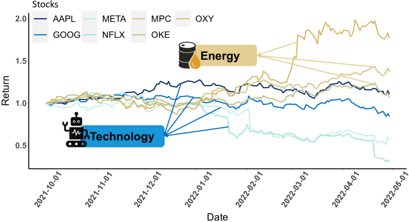
However, stock market analysis based on deep learning faces two important requirements. First, multi-order dynamics of stock movements need to be incorporated. Price movements are often correlated within a specific group of stocks, e.g., companies of the same industry sector that are affected by the same government policies, laws, and tax rates. For instance, as shown in Fig. 1, in early 2022, prices for US technology stocks (APPL (Apple), META (Facebook), GOOG (Google), NFLX (Netflix)) went down due to the general economic trend (inflation, increased interest rates), whereas stocks in the energy sector, like MPC, OKE, or OXY, experienced upward trends due to oil shortages caused by the Russia-Ukraine war. Second, the internal dynamics per stock need to be incorporated. In practice, even when considering highly correlated stocks, there is commonly still some individual behaviour. For example, in Fig. 1, APPL and GOOG stocks decrease less severely than META and NFLX, as the former companies (Apple, Google) maintain a wider and more sustainable portfolio compared to the latter two (Facebook, Netflix) (New York Times, 2022).
Existing work provides only limited support for these requirements. First, to incorporate multi-order dynamics of stock markets, RNNs can be combined with graph neural networks (GNNs) (Kim et al., 2019). Here, state-of-the-art solutions adopt hypergraphs, in which an edge captures the correlation of multiple stocks (Sawhney et al., 2020; Sawhney et al., 2021). Yet, these approaches rely on the Fourier basis in the convolution, which implies costly matrix operations and does not maintain the localization well. This raises the question of how to achieve an efficient and effective convolution process for hypergraphs (Challenge 1). Moreover, state-of-the-art approaches apply a single RNN to all stocks, thereby ignoring their individual behaviour. The reason being that maintaining a separate model per stock would be intractable with existing techniques. This raises the question of how to model the internal dynamics of stocks efficiently (Challenge 2).
In this work, we address the above challenges by proposing Efficient Stock Integration with Temporal Generative Filters and Wavelet Hypergraph Attentions (ESTIMATE), a profit-driven framework for quantitative trading. Based on the aforementioned idea of adopting hypergraphs to capture non-pairwise correlations between stocks, the framework includes two main contributions:
-
•
We present temporal generative filters that implement a hybrid attention-based LSTM architecture to capture the stocks’ individual behavioural patterns (Challenge 2). These patterns are then fed to hypergraph convolution layers to obtain spatio-temporal embeddings that are optimized with respect to the potential of the stocks for short-term profit.
-
•
We propose a mechanism that combines the temporal patterns of stocks with spatial convolutions through hypergraph attention, thereby integrating the internal dynamics and the multi-order dynamics. Our convolution process uses the wavelet basis, which is efficient and also effective in terms of maintaining the localization (Challenge 1).
To evaluate our approach, we report on backtesting experiments for the US market. Here, we try to simulate the real trading actions with a strategy for portfolio management and risk control. The results demonstrate the robustness of our technique compared to existing approaches in terms of stability and return. Our source code and data are available (Github, 2022).
The remainder of the paper is organised as follows. § 2 introduces the problem statement and gives an overview of our approach. We present our new techniques, the temporal generative filters and wavelet hypergraph attentions, in § 3 and § 4. § 5 presents experiments, § 6 reviews related works, and § 7 concludes the paper.
2. Model and approach
2.1. Problem Formulation
In this section, we formulate the problem of predicting the trend of a stock in the short term. We start with some basic notions.
OHCLV data. At timestep , the open-high-low-close-volume (OHLCV) record for a stock is a vector . It denotes the open, high, low, and close price, and the volume of shares that have been traded within that timestep, respectively.
Relative price change. We denote the relative close price change between two timesteps of stock by . The relative price change normalizes the market price variety between different stocks in comparison to the absolute price change.
Following existing work on stock market analysis (Sawhney et al., 2020; Feng et al., 2019a), we focus on the prediction of the change in price rather than the absolute value. The reason being that the timeseries of stock prices are non-stationary, whereas their changes are stationary (Li et al., 2020). Also, this avoids the problem that forecasts often lag behind the actual value (Kim et al., 2019; Hu et al., 2018). We thus define the addressed problem as follows:
Problem 1 (Stock Movement Prediction).
Given a set of stocks and a lookback window of trading days of historic OHLCV records for each stock , the problem of Stock Movement Prediction is to predict the relative price change for each stock in a short-term lookahead window .
We formulate the problem as a short-term regression for several reasons. First, we consider a lookahead window over next-day prediction to be robust against random market fluctuations (Zhang et al., 2017). Second, we opt for short-term prediction, as an estimation of the long-term trend is commonly considered infeasible without the integration of expert knowledge on the intrinsic value of companies and on macroeconomic effects. Third, we focus on a regression problem instead of a classification problem to incorporate the magnitude of a stock’s trend, which is important for interpretation (Gu et al., 2020).
2.2. Design Principles
We argue that any solution to the above problem shall satisfy the following requirements:
-
•
R1: Multi-dimensional data integration: Stock market data is multivariate, covering multiple stocks and multiple features per stock. A solution shall integrate these data dimensions and support the construction of additional indicators from basic OHCLV data.
-
•
R2: Non-stationary awareness: The stock market is driven by various factors, such as socio-economic effects or supply-demand changes. Therefore, a solution shall be robust against non-predictable behaviour of the market.
-
•
R3: Analysis of multi-order dynamics: The relations between stocks are complex (e.g., companies may both, cooperate and compete) and may evolve over time. A solution thus needs to analyse the multi-order dynamics in a market.
-
•
R4: Analysis of internal dynamics: Each stock also shows some individual behaviour, beyond the multi-order correlations induced by market segments. A solution therefore needs to analyse and integrate such behaviour for each stock.
2.3. Approach Overview
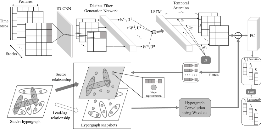
To address the problem of stock movement prediction in the light of the above design principles, we propose the framework shown in Fig. 2. It takes historic data in the form of OHCLV records and derives a model for short-term prediction of price changes per stock.
Our framework incorporates requirement R1 by first extracting the historic patterns per stock using a temporal attention LSTM. Here, the attention mechanism is used along with a 1D-CNN to assess the impact of the previous timesteps. In addition to the OHCLV data, we employ technical indicators to mitigate the impact of noisy market behaviour, thereby addressing requirement R2. Moreover, we go beyond the state of the art by associating the core LSTM parameters with a learnable vector for each stock. It serves as a memory that stores its individual information (requirement R4) and results in a system of temporal generative filters. We explain the details of these filters in § 3.
To handle multi-order dynamics (requirement R3), we model the market with an industry-based hypergraph, which naturally presents non-pairwise relationships. We then develop a wavelet convolution mechanism, which leverages the wavelet basis to achieve a simpler convolution process than existing approaches. We apply a regression loss to steer the model to predict the short-term trend of each stock price. The details of our proposed hypergraph convolution process are given in § 4.
3. Temporal Generative Filters
This section describes our temporal generative filters used to capture the internal dynamics of stocks.
Technical indicators. We first compute various technical indicators from the input data in order to enrich the data and capture the historical context of each stock. These indicators, summarized in Table 1, are widely used in finance. For each stock, we concatenate these indicators to form a stock price feature vector on day . This vector is then forwarded through a multi-layer perceptron (MLP) layer to modulate the input size.
| Type | Indicators |
|---|---|
| Trend Indicators | Arithmetic ratio, Close Ratio, Close SMA, |
| Volume SMA, Close EMA, Volume EMA, ADX | |
| Oscillator Indicators | RSI, MACD, Stochastics, MFI |
| Volatility Indicators | ATR, Bollinger Band, OBV |
Local trends. To capture local trends in stock patterns, we employ convolutional neural networks (CNN). By compressing the length of the series of stock features, they help to mitigate the issue of long-term dependencies. As each feature is a one-dimensional timeseries, we apply one-dimensional filters (1D-CNN) over all timesteps:
| (1) |
where represent the input feature at the neuron of layer ; is the corresponding bias; is the kernel from the neuron at layer to the neuron at layer ; and is the output of the neuron at layer .
Temporal LSTM extractor with Distinct Generative Filter. After forwarding the features through the CNNs, we use an LSTM to capture the temporal dependencies, exploiting its ability to memorize long-term information. Given the concatenated feature of the stocks at time , we feed the feature through the LSTM layer:
| (2) |
where is the hidden state for day and d is the hidden state dimension. The specific computation in each LSTM unit includes:
As mentioned, existing approaches apply the same LSTM to the historical data of different stocks, which results in the learned set of filters () representing the average temporal dynamics. This is insufficient to capture each stock’s distinct behaviour (Challenge 2).
A straightforward solution would be to learn and store a set of LSTM filters, one for each stock. Yet, such an approach quickly becomes intractable, especially when the number of stocks is large.
In our model, we overcome this issue by proposing a memory-based mechanism onto the LSTM network to learn the individual patterns per stock, while not expanding the core LSTM. Specifically, we first assign to each stock a memory in the form of a learnable m-dimensional vector, . Then, for each entity, we feed the memory through a Distinct Generative Filter, denoted by DGF, to obtain the weights () of the LSTM network for each stock:
| (3) |
Note that DGF can be any neural network architecture, such as a CNN or an MLP. In our work, we choose a 2-layer MLP as DGF, as it is simple yet effective. As the DGF is required to generate a set of eight filters from , we generate a concatenation of the filters and then obtain the results by splitting. Finally, replacing the common filters by the specific ones for each stock in Eq. 2, we have:
| (4) |
where is the hidden feature of each stock .
To increase the efficiency of the LSTM, we apply a temporal attention mechanism to guide the learning process towards important historical features. The attention mechanism attempts to aggregate temporal hidden states from previous days into an overall representation using learned attention weights:
| (5) |
where is a linear transformation, are the attention weights using softmax. To handle the non-stationary nature of the stock market, we leverage the Hawkes process (Bacry et al., 2015), as suggested for financial timeseries in (Sawhney et al., 2021), to enhance the temporal attention mechanism in Eq. 5. The Hawkes process is a “self-exciting” temporal point process, where some random event “excites” the process and increases the chance of a subsequent other random event (e.g., a crises or policy change). To realize the Hawke process, the attention mechanism also learns an excitation parameter of the day and a corresponding decay parameter :
| (6) |
Finally, we concatenate the extracted temporal feature of each stock to form , where is the number of stocks and is the embedding dimension.
4. High-order market learning with wavelet hypergraph attentions
To model the groupwise relations between stocks, we aggregate the learned temporal patterns of each stock over a hypergraph that represents multi-order relations of the market.
Industry hypergraph. To model the interdependence between stocks, we first initialize a hypergraph based on the industry of the respective companies. Mathematically, the industry hypergraph is denoted as , where is the set of stocks and is the set of hyperedges; each hyperedge connects the stocks that belong to the same industry. The hyperedge is also assigned a weight that reflects the importance of the industry, which we derive from the market capital of all related stocks.
Price correlation augmentation. Following the Efficient Market Hypothesis (Malkiel, 1989), fundamentally correlated stocks maintain similar price patterns, which can be used to reveal the missing endogenous relations in addition to the industry assignment. To this end, for the start of each training and testing period, we calculate the price correlation between the stocks using the historical price of the last 1-year period. We employ the lead-lag correlation and the clustering method proposed in (Bennett et al., 2021) to simulate the lag of the stock market, where a leading stock affects the trend of the rests. Then, we form hyperedges from the resulting clusters and add them to . The hyperedge weight is, again, derived from the total market capital of the related stocks. We denote the augmented hypergraph by , with A and W being the hypergraph incidence matrix and the hyperedge weights, respectively.
Wavelet Hypergraph Convolution. To aggregate the extracted temporal information of the individual stocks, we develop a hypergraph convolution mechanism on the obtained hypergraph , which consists of multiple convolution layers. At each layer , the latent representations of the stocks in the previous layer are aggregated by a convolution operator HConv(·) using the topology of to generate the current layer representations :
| (7) |
where and with being the number of stocks and as the dimension of the layer-wise latent feature; is a learnable weight matrix for the layer. Following (Yadati et al., 2019), the convolution process requires the calculation of the hypergraph Laplacian , which serves as a normalized presentation of :
| (8) |
where and are the diagonal matrices containing the vertex and hyperedge degrees, respectively. For later usage, we denote by . As is a positive semi-definite matrix, it can be diagonalized as: , where is the diagonal matrix of non-negative eigenvalues and is the set of orthonormal eigenvectors.
Existing work leverages the Fourier basis (Yadati et al., 2019) for this factorization process. However, using the Fourier basis has two disadvantages: (i) the localization during convolution process is not well-maintained (Xu et al., 2019), and (ii) it requires the direct eigen-decomposition of the Laplacian matrix, which is costly for a complex hypergraph, such as those faced when modelling stock markets (Challenge 1). We thus opt to rely on the wavelet basis (Xu et al., 2019), for two reasons: (i) the wavelet basis represents the information diffusion process (Sun et al., 2021), which naturally implements localized convolutions of the vertex at each layer, and (ii) the wavelet basis is much sparser than the Fourier basis, which enables more efficient computation.
Applying the wavelet basis, let be a set of wavelets with scaling parameter . Then, we have as the heat kernel matrix. The hypergraph convolution process for each vertex is computed by:
| (9) |
where is the filter and is its corresponding spectral transformation. Based on the Stone-Weierstrass theorem (Xu et al., 2019), the graph wavelet can be polynomially approximated by:
| (10) |
where is the polynomial order of the approximation.
The approximation facilitates the calculation of without the eigen-decomposition of . Applying it to Eq. 10 and Eq. 7 and choosing LeakyReLU (Agarap, 2018) as the activation function, we have:
| (11) |
To capture the varying degree of influence each relation between stocks on the temporal price evolution of each stock, we also employ an attention mechanism (Sawhney et al., 2021). This mechanism learns to adaptively weight each hyperedge associated with a stock based on its temporal features. For each node and its associated hyperedge , we compute an attention coefficient using the stock’s temporal feature and the aggregated hyperedge features , quantifying how important the corresponding relation is to the stock :
| (12) |
where is a single-layer feed forward network, is concatenation operator and represents a learned linear transform. is the neighbourhood set of the stock , which is derived from the constructed hypergraph . The attention-based learned hypergraph incidence matrix is then used instead of the original in Eq. 11 to learn intermediate representations of the stocks. The representation of the hypergraph is denoted by , which is concatenated with the temporal feature to maintain the stock individual characteristic (Challenge 2), which then goes through the MLP for dimension reduction to obtain the final prediction:
| (13) |
Finally, we use the popular root mean squared error (RMSE) to directly encourage the output to capture the actual relative price change in the short term of each stock , with being the lookahead window size (with a default value of five).
5. Empirical Evaluation
| Model | Phase #1 | Phase #2 | Phase #3 | Phase #4 | Phase #5 | Phase #6 | Phase #7 | Phase #8 | Phase #9 | Phase #10 | Phase #11 | Phase #12 | Mean | |
|---|---|---|---|---|---|---|---|---|---|---|---|---|---|---|
| Return | LSTM | 0.064 | 0.057 | 0.028 | 0.058 | 0.036 | -0.032 | 0.059 | -0.139 | 0.125 | 0.100 | 0.062 | 0.008 | 0.036 |
| ALSTM | 0.056 | 0.043 | 0.022 | 0.053 | 0.009 | -0.068 | 0.036 | -0.121 | 0.115 | 0.097 | 0.066 | 0.009 | 0.026 | |
| HATS | 0.102 | 0.031 | -0.003 | 0.042 | 0.062 | 0.067 | 0.092 | -0.074 | 0.188 | 0.132 | 0.063 | -0.059 | 0.054 | |
| LSTM-RGCN | 0.089 | 0.051 | 0.005 | -0.006 | 0.077 | 0.019 | 0.088 | -0.121 | 0.155 | 0.107 | 0.038 | -0.032 | 0.039 | |
| RSR | 0.065 | 0.043 | -0.009 | -0.016 | 0.014 | -0.007 | 0.059 | -0.113 | 0.089 | 0.056 | 0.038 | -0.052 | 0.014 | |
| STHAN-SR | 0.108 | 0.074 | 0.024 | 0.016 | 0.052 | 0.085 | 0.090 | -0.105 | 0.158 | 0.107 | 0.058 | -0.008 | 0.055 | |
| HIST | 0.080 | 0.020 | -0.020 | -0.030 | -0.050 | 0.010 | -0.030 | 0.020 | 0.200 | 0.100 | 0.020 | -0.050 | 0.022 | |
| ESTIMATE | 0.109 | 0.080 | 0.025 | 0.105 | 0.051 | 0.135 | 0.149 | 0.124 | 0.173 | 0.065 | 0.147 | 0.057 | 0.102 | |
| IC | LSTM | -0.014 | -0.030 | -0.016 | 0.006 | 0.020 | -0.034 | -0.006 | 0.014 | -0.002 | -0.039 | 0.022 | -0.023 | -0.009 |
| ALSTM | -0.024 | -0.025 | 0.025 | -0.009 | 0.029 | -0.018 | -0.033 | -0.024 | 0.045 | -0.046 | 0.016 | -0.015 | -0.007 | |
| HATS | 0.013 | -0.011 | -0.006 | -0.005 | -0.018 | 0.029 | 0.027 | -0.002 | 0.010 | -0.017 | -0.028 | -0.012 | -0.002 | |
| LSTM-RGCN | -0.019 | 0.020 | 0.024 | 0.021 | -0.005 | 0.021 | 0.032 | 0.035 | -0.086 | 0.043 | -0.005 | 0.030 | 0.009 | |
| RSR | 0.008 | -0.009 | -0.003 | -0.017 | -0.009 | 0.018 | 0.011 | -0.005 | -0.036 | 0.018 | -0.058 | 0.003 | -0.007 | |
| STHAN-SR | 0.025 | -0.015 | -0.016 | -0.029 | 0.000 | 0.018 | 0.022 | 0.000 | -0.010 | 0.009 | 0.007 | -0.013 | 0.000 | |
| HIST | 0.003 | 0.000 | 0.005 | -0.010 | 0.006 | 0.008 | 0.005 | -0.017 | 0.006 | 0.009 | 0.011 | 0.006 | 0.003 | |
| ESTIMATE | 0.037 | 0.080 | 0.153 | 0.010 | 0.076 | 0.080 | 0.080 | 0.011 | 0.127 | 0.166 | 0.010 | 0.131 | 0.080 | |
| Rank_IC | LSTM | -0.151 | -0.356 | -0.289 | 0.089 | 0.186 | -1.091 | -0.151 | 0.201 | -0.019 | -0.496 | 0.259 | -0.397 | -0.185 |
| ALSTM | -0.211 | -0.266 | 0.409 | -0.099 | 0.182 | -0.289 | -0.476 | -0.243 | 0.242 | -0.323 | 0.094 | -0.174 | -0.096 | |
| HATS | 0.169 | -0.156 | -0.139 | -0.063 | -0.408 | 0.517 | 0.333 | -0.032 | 0.085 | -0.344 | -0.547 | -0.135 | -0.060 | |
| LSTM-RGCN | -0.271 | 0.210 | 0.223 | 0.152 | -0.035 | 0.279 | 0.261 | 0.273 | -0.416 | 0.329 | -0.036 | 0.354 | 0.110 | |
| RSR | 0.151 | -0.159 | -0.051 | -0.213 | -0.107 | 0.282 | 0.135 | -0.090 | -0.292 | 0.175 | -0.541 | 0.040 | -0.056 | |
| STHAN-SR | 0.690 | -0.357 | -0.365 | -0.714 | 0.008 | 0.369 | 0.523 | 0.005 | -0.265 | 0.169 | 0.141 | -0.276 | -0.006 | |
| HIST | 0.085 | -0.008 | 0.125 | -0.225 | 0.192 | 0.204 | 0.107 | -0.328 | 0.174 | 0.256 | 0.215 | 0.157 | 0.080 | |
| ESTIMATE | 0.386 | 0.507 | 1.613 | 0.059 | 0.284 | 0.585 | 0.412 | 0.062 | 0.704 | 0.936 | 0.054 | 0.595 | 0.516 | |
| ICIR | LSTM | -0.010 | -0.036 | -0.007 | 0.010 | 0.016 | -0.038 | 0.004 | 0.010 | 0.011 | -0.041 | 0.021 | -0.010 | -0.006 |
| ALSTM | -0.057 | -0.041 | 0.030 | -0.012 | 0.033 | -0.015 | -0.028 | -0.034 | 0.057 | -0.053 | 0.009 | -0.002 | -0.009 | |
| HATS | 0.023 | -0.014 | 0.010 | 0.001 | -0.016 | 0.033 | 0.035 | 0.020 | 0.023 | -0.005 | -0.042 | -0.034 | 0.003 | |
| LSTM-RGCN | -0.033 | 0.012 | 0.022 | 0.027 | -0.009 | 0.028 | 0.047 | 0.051 | -0.085 | 0.054 | -0.006 | 0.039 | 0.012 | |
| RSR | 0.031 | -0.018 | -0.005 | -0.033 | -0.009 | 0.029 | 0.001 | -0.007 | -0 .019 | 0.017 | -0.072 | -0.031 | -0.010 | |
| STHAN-SR | 0.018 | -0.011 | -0.016 | -0.021 | 0.005 | 0.016 | 0.023 | 0.008 | -0.003 | 0.004 | 0.009 | -0.007 | 0.002 | |
| HIST | 0.004 | -0.002 | -0.006 | -0.001 | 0.007 | 0.001 | 0.005 | -0.014 | 0.009 | 0.009 | 0.021 | 0.010 | 0.004 | |
| ESTIMATE | 0.033 | 0.081 | 0.148 | 0.032 | 0.076 | 0.103 | 0.064 | 0.058 | 0.103 | 0.142 | 0.020 | 0.098 | 0.080 | |
| Rank_ICIR | LSTM | -0.100 | -0.364 | -0.110 | 0.140 | 0.141 | -0.984 | 0.094 | 0.168 | 0.117 | -0.525 | 0.227 | -0.172 | -0.114 |
| ALSTM | -0.423 | -0.344 | 0.415 | -0.134 | 0.202 | -0.192 | -0.313 | -0.343 | 0.306 | -0.377 | 0.047 | -0.019 | -0.098 | |
| HATS | 0.234 | -0.155 | 0.179 | 0.013 | -0.221 | 0.511 | 0.340 | 0.270 | 0.194 | -0.076 | -0.525 | -0.372 | 0.033 | |
| LSTM-RGCN | -0.387 | 0.111 | 0.197 | 0.170 | -0.058 | 0.313 | 0.284 | 0.326 | -0.354 | 0.318 | -0.034 | 0.427 | 0.109 | |
| RSR | 0.378 | -0.353 | -0.053 | -0.285 | -0.065 | 0.326 | 0.010 | -0.081 | -0.114 | 0.131 | -0.428 | -0.288 | -0.068 | |
| STHAN-SR | 0.435 | -0.211 | -0.310 | -0.573 | 0.107 | 0.386 | 0.478 | 0.271 | -0.068 | 0.075 | 0.230 | -0.149 | 0.056 | |
| HIST | 0.079 | -0.044 | -0.144 | -0.020 | 0.205 | 0.018 | 0.122 | -0.289 | 0.236 | 0.229 | 0.356 | 0.209 | 0.080 | |
| ESTIMATE | 0.315 | 0.446 | 1.344 | 0.178 | 0.307 | 0.587 | 0.329 | 0.311 | 0.541 | 0.885 | 0.100 | 0.488 | 0.486 | |
| Prec@N | LSTM | 0.542 | 0.553 | 0.581 | 0.471 | 0.456 | 0.569 | 0.440 | 0.547 | 0.588 | 0.615 | 0.554 | 0.608 | 0.544 |
| ALSTM | 0.583 | 0.585 | 0.550 | 0.471 | 0.514 | 0.575 | 0.431 | 0.556 | 0.650 | 0.518 | 0.497 | 0.627 | 0.546 | |
| HATS | 0.624 | 0.651 | 0.597 | 0.495 | 0.551 | 0.642 | 0.532 | 0.619 | 0.542 | 0.550 | 0.529 | 0.690 | 0.585 | |
| LSTM-RGCN | 0.565 | 0.589 | 0.600 | 0.505 | 0.505 | 0.628 | 0.522 | 0.583 | 0.517 | 0.538 | 0.566 | 0.592 | 0.559 | |
| RSR | 0.587 | 0.531 | 0.608 | 0.455 | 0.465 | 0.619 | 0.473 | 0.608 | 0.553 | 0.618 | 0.590 | 0.676 | 0.565 | |
| STHAN-SR | 0.554 | 0.614 | 0.573 | 0.463 | 0.562 | 0.611 | 0.530 | 0.575 | 0.553 | 0.626 | 0.534 | 0.510 | 0.559 | |
| HIST | 0.691 | 0.625 | 0.476 | 0.512 | 0.452 | 0.561 | 0.548 | 0.634 | 0.463 | 0.615 | 0.395 | 0.605 | 0.548 | |
| ESTIMATE | 0.619 | 0.631 | 0.673 | 0.524 | 0.540 | 0.739 | 0.568 | 0.669 | 0.611 | 0.679 | 0.547 | 0.724 | 0.627 |
In this section, we empirically evaluate our framework based on four research questions, as follows:
-
(RQ1)
Does our model outperform the baseline methods?
-
(RQ2)
What is the influence of each model component?
-
(RQ3)
Can our model be interpreted in a qualitative sense?
-
(RQ4)
Is our model sensitive to hyperparameters?
Below, we first describe the experimental setting (§ 5.1). We then present our empirical evaluations, including an end-to-end comparison (§ 5.2), a qualitative study (§ 5.4), an ablation test (§ 5.3), and an examination of the hyperparameter sensitivity (§ 5.5).
5.1. Setting
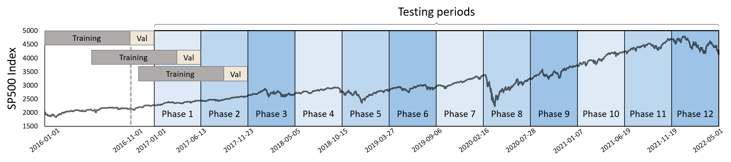
Datasets. We evaluate our approach based on the US stock market. We gathered historic price data and the information about industries in the S&P 500 index from the Yahoo Finance database (Yahoo Finance, 2022), covering 2016/01/01 to 2022/05/01 (1593 trading days). Overall, while the market witnessed an upward trend in this period, it also experienced some considerable correction in 2018, 2020, and 2022. We split the data of this period into 12 phases with varying degrees of volatility, with the period between two consecutive phases being 163 days. Each phase contains 10 month of training data, 2 month of validation data, and 6 month of testing data (see Fig. 3).
Metrics. We adopt the following evaluation metrics: To thoroughly evaluate the performance of the techniques, we employ the following metrics:
-
•
Return: is the estimated profit/loss ratio that the portfolio achieves after a specific period, calculated by , with and being the net asset value of the portfolio before and after the period.
-
•
Information Coefficient (IC): is a coefficient that shows how close the prediction is to the actual result, computed by the average Pearson correlation coefficient.
-
•
Information ratio based IC (ICIR): The information ratio of the IC metric, calculated by
-
•
Rank Information Coefficient (Rank_IC): is the coefficient based on the ranking of the stocks’ short-term profit potential, computed by the average Spearman coefficient (Myers and Sirois, 2004).
-
•
Rank_ICIR: Information ratio based Rank_IC (ICIR): The information ratio of the Rank_IC metric, calculated by:
-
•
Prec@N: evaluates the precision of the top N short-term profit predictions from the model. This way, we assess the capability of the techniques to support investment decisions.
Baselines. We compared the performance of our technique with that of several state-of-the-art baselines, as follows:
-
•
LSTM: (Hochreiter and Schmidhuber, 1997) is a traditional baseline which leverages a vanilla LSTM on temporal price data.
-
•
ALSTM: (Feng et al., 2019a) is a stock movement prediction framework that integrates the adversarial training and stochasticity simulation in an LSTM to better learn the market dynamics.
-
•
HATS: (Kim et al., 2019) is a stock prediction framework that models the market as a classic heterogeneous graph and propose a hierarchical graph attention network to learn a stock representation to classify next-day movements.
-
•
LSTM-RGCN: (Li et al., 2020) is a graph-based prediction framework that constructs the connection among stocks with their price correlation matrix and learns the spatio-temporal relations using a GCN-based encoder-decoder architecture.
-
•
RSR: (Feng et al., 2019b) is a stock prediction framework that combines Temporal Graph Convolution with LSTM to learn the stocks’ relations in a time-sensitive manner.
-
•
HIST: (Xu et al., 2021) is a graph-based stock trend forecasting framework that follows the encoder-decoder paradigm in attempt to capture the shared information between stocks from both predefined concepts as well as revealing hidden concepts.
-
•
STHAN-SR: (Sawhney et al., 2021) is a deep learning-based framework that also models the complex relation of the stock market as a hypergraph and employs vanilla hypergraph convolution to learn directly the stock short-term profit ranking.
Trading simulation. We simulate a trading portfolio using the output prediction of the techniques. At each timestep, the portfolio allocates an equal portion of money for k stocks, as determined by the prediction. We simulate the risk control by applying a trailing stop level of 7% and profit taking level of 20% for all positions. We ran the simulation 1000 times per phase and report average results.
Reproducibility environment. All experiments were conducted on an AMD Ryzen ThreadRipper 3.8 GHz system with 128 GB of main memory and four RTX 3080 graphic cards. We used Pytorch for the implementation and Adam as gradient optimizer.
5.2. End-to-end comparisons
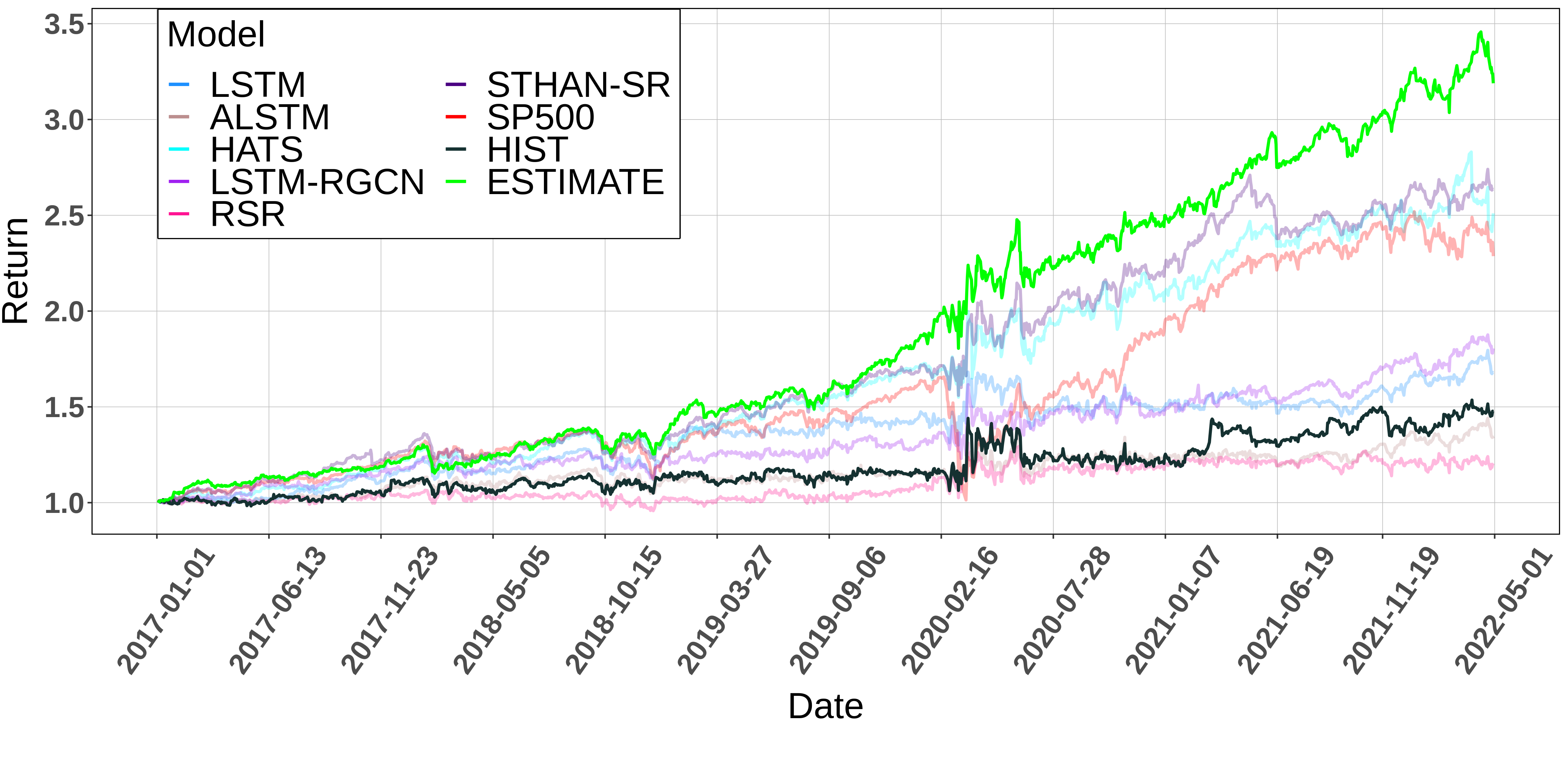
To answer research question RQ1, we report in Table 2 an end-to-end comparison of our approach (ESTIMATE) against the baseline methods. We also visualize the average accumulated return of the baselines and the S&P 500 index during all 12 phases in Fig. 4.
In general, our model outperforms all baseline methods across all datasets in terms of Return, IC, Rank_IC and Prec@10. Our technique consistently achieves a positive return and an average Prec@10 of 0.627 over all 12 phases; and performs significant better than the S&P 500 index with higher overall return. STHAN-SR is the best method among the baselines, yielding a high Return in some phases (#1, #2, #5, #10). This is because STHAN-SR, similar to our approach, models the multi-order relations between the stocks using a hypergraph. However, our technique still outperforms STHAN-SR by a considerable margin for the other periods, including the ranking metric Rank_IC even though our technique does not aim to learn directly the stock rank, like STHAN-SR.
Among the other baseline, models with a relational basis like RSR, HATS, and LSTM-RGCN outperform vanilla LSTM and ALSTM models. However, the gap between classic graph-based techniques like HATS and LSTM-RGCN is small. This indicates that the complex relations in a stock market shall be modelled. An interesting finding is that all the performance of the techniques drops significantly during phase #3 and phase #4, even though the market moves sideways. This observation highlights issues of prediction algorithm when there is no clear trend for the market.
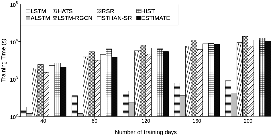
The training times for these techniques are shown in Fig. 5, where we consider the size of training set ranging from 40 to 200 days. As expected, the graph-based techniques (HATS, LSTM-RGCN, RSR, STHAN-R, HIST and ESTIMATE) are slower than the rest, due to the trade-off between accuracy and computation time. Among the graph-based techniques, there is no significant difference between the techniques using classic graphs (HATS, LSTM-RGCN) and those using hypergraphs (ESTIMATE, STHAN-R). Our technique ESTIMATE is faster than STHAN-R by a considerable margin and is one of the fastest among the graph-based baselines, which highlights the efficiency of our wavelet convolution scheme compared to the traditional Fourier basis.
5.3. Ablation Study
To answer question RQ2, we evaluated the importance of individual components of our model by creating four variants: (EST-1) This variant does not employ the hypergraph convolution, but directly uses the extracted temporal features to predict the short-term trend of stock prices. (EST-2) This variant does not employ the generative filters, but relies on a common attention LSTM by existing approaches. (EST-3) This variant does not apply the price-correlation based augmentation, as described in § 4. It employs solely the industry-based hypergraph as input. (EST-4) This variant does not employ the wavelet basis for hypergraph convolution, as introduced in § 4. Rather, the traditional Fourier basis is applied.
| Metric | ESTIMATE | EST-1 | EST-2 | EST-3 | EST-4 |
|---|---|---|---|---|---|
| Return | 0.102 | 0.024 | 0.043 | 0.047 | 0.052 |
| IC | 0.080 | 0.013 | 0.020 | 0.033 | 0.020 |
| RankIC | 0.516 | 0.121 | 0.152 | 0.339 | 0.199 |
| Prec@N | 0.627 | 0.526 | 0.583 | 0.603 | 0.556 |
Table 3 presents the results for several evaluation metrics, averaged over all phases due to space constraints. We observe that our full model ESTIMATE outperforms the other variants, which provides evidence for the the positive impact of each of its components. In particular, it is unsurprising that the removal of the relations between stocks leads to a significant degradation of the final result (approximately 75% of the average return) in EST-1. A similar drop of the average return can be seen for EST-2 and EST-3, which highlights the benefits of using generati +ve filters over a traditional single LSTM temporal extractor (EST-2); and of the proper construction of the representative hypergraph (EST-3). Also, the full model outperforms the variant EST-4 by a large margin in every metric. This underlines the robustness of the convolution with the wavelet basis used in ESTIMATE over the traditional Fourier basis that is used in existing work.
5.4. Qualitative Study
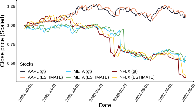
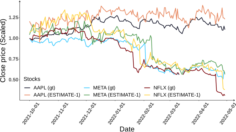
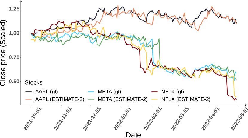
We answer research question RQ3 by visualizing in Fig. 6 the prediction results of our technique ESTIMATE for the technology stocks APPL and META from 01/10/2021 to 01/05/2022. We also compare ESTIMATE’s performance to the variant that does not consider relations between stocks (EST-1) and the variant that does not employ temporal generative filters (EST-2). This way, we illustrate how our technique is able to handle Challenge 1 and Challenge 2.
The results indicate that modelling the complex multi-order dynamics of a stock market (Challenge 1) helps ESTIMATE and EST-2 to correctly predict the downward trend of technology stocks around the start of 2022; while the prediction of EST-1, which uses the temporal patterns of each stock, suffers from a significant delay. Also, the awareness of internal dynamics of ESTIMATE due to the usage of generative filters helps our technique to differentiate the trend observed for APPL from the one of META, especially at the start of the correction period in January 2022.
5.5. Hyperparameter sensitivity
This experiment addresses question RQ4 on the hyperparameter sensitivity. Due to space limitations, we focus on the most important hyperparameters. The backtesting period of this experiment is set from 01/07/2021 to 01/05/2022 for the same reason.
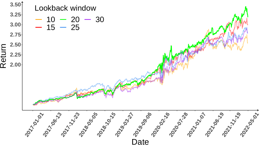

Lookback window length T. We analyze the prediction performance of ESTIMATE when varying the length T of the lookback window in Fig. 7. It can be observed that the best window length is 20, which coincides with an important length commonly used by professional analyses strategies (Adam et al., 2016). The performance drops quickly when the window length is less or equal than 10, due to the lack of information. On the other hand, the performance also degrades when the window length increases above 25. This shows that even when using an LSTM to mitigate the vanishing gradient issue, the model cannot handle very long sequences.
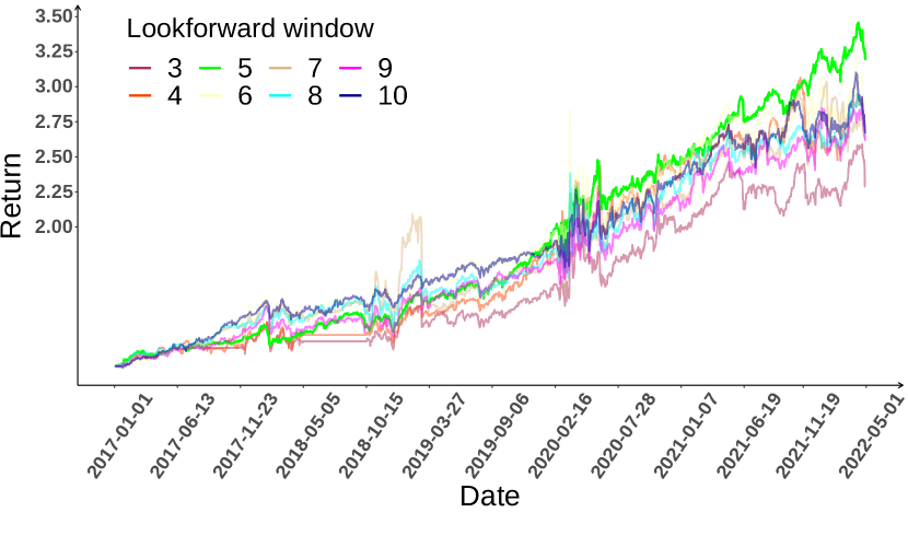
Lookahead window length w. We consider different lengths w of the lookahead window (Fig. 7) and observe that ESTIMATE achieves the best performance for a window of length 5. The results degrade significantly when w exceeds 10. This shows that our model performs well for short-term prediction, it faces issues when considering a long-term view.
Number of selected top-k stocks. We analyze the variance in the profitability depending on the number of selected top-k stocks from the ranking in Fig. 7. We find that ESTIMATE performs generally well, while the best results are obtained for k = 10.
6. Related Work
Traditional Stock Modelling. Traditional techniques often focus on numerical features (Liou et al., 2021; Ruiz et al., 2012), referred to as technical indicators, such as the Moving Average (MA) or the Relative Strength Index (RSI). The features are combined with classical timeseries models, such as ARIMA (Piccolo, 1990), to model the stock movement (Ariyo et al., 2014). However, such techniques often require the careful engineering by experts to identify effective indicator combinations and thresholds. Yet, these configurations are often not robust against market changes.
For individual traders, they often engineer rules based on a specific set of technical indicators (which indicate the trading momentum) to find the buying signals. For instance, a popular strategy is to buy when the moving average of length 5 (MA5) cross above the moving average of length 20 (MA20), and the Moving Average Convergence Divergence (MACD) is positive. However, the engineering of the specific features requires the extensive expertise and experiment of the traders in the market. Also, the traders must continuously tune and backtest the strategy, as the optimized strategy is not only different from the markets but also keeps changing to the evolving of the market. Last but not least, it is exhaustive for the trader to keep track of a large number of indicators of a stock, as well as the movement of multiple stocks in real time. Due to these drawbacks, quantitative trading with the aid of the AI emerges in recent years, especially with the advances of deep neural network (DNN).
DNN-based Stock Modelling. Recent techniques leverage advances in deep learning to capture the non-linear temporal dynamics of stock prices through high-level latent features (Ren and Malik, 2019; Huynh et al., 2021; Bendre et al., 2021). Earlier techniques following this paradigm employ recurrent neural networks (RNN) (Nelson et al., 2017) or convolutional neural networks (CNN) (Tsantekidis et al., 2017) to model a single stock price and predict its short-term trend. Other works employ deep reinforcement learning (DRL), the combination of deep learning with reinforcement learning (RL), a subfield of sequential decision-making. For instance, the quantitative trading problem can be formulated as a Markov decision process (Liu et al., 2021) and be addressed by well-known DRL algorithms (e.g. DQN, DDPG (Lillicrap et al., 2016)). However, these techniques treat the stocks independently and lack a proper scheme to consider the complex relations between stocks in the market.
Graph-based Stock Modelling. Some state-of-the-art techniques address the problem of correlations between stocks and propose graph-based solutions to capture the inter-stock relations. For instance, the market may be modelled as a heterogeneous graph with different type of pairwise relations (Kim et al., 2019), which is then used in an attention-based graph convolution network (GCN) (Duong et al., 2023; Nguyen et al., 2022b, 2021b, 2020; Tam et al., 2021; Trung et al., 2020) to predict the stock price and market index movement. Similarly, a market graph may be constructed and an augmented GCN with temporal convolutions can be employed to learn, at the same time, the stock movement and stock relation evolution (Li et al., 2020). The most recent techniques (Feng et al., 2019b; Sawhney et al., 2021) are based on the argument that the stock market includes multi-order relations, so that the market should be modelled using hypergraphs. Specifically, external knowledge from knowledge graphs enables the construction of a market hypergraph (Sawhney et al., 2021), which is used in a spatiotemporal attention hypergraph network to learn interdependences of stocks and their evolution. Then, a ranking of stocks based on short-term profit is derived.
Different from previous work, we propose a market analysis framework that learns the complex multi-order correlation of stocks derived from a hypergraph representation. We go beyond the state of the art ((Feng et al., 2019b; Sawhney et al., 2021)) by proposing temporal generative filters that implement a memory-based mechanism to recognize better the individual characteristics of each stock, while not over-parameterizing the core LSTM model. Also, we propose a new hypergraph attention convolution scheme that leverages the wavelet basis to mitigate the high complexity and dispersed localization faced in previous hypergraph-based approaches.
7. Conclusion
In this paper, we address two unique characteristics of the stock market prediction problem: (i) multi-order dynamics which implies strong non-pairwise correlations between the price movement of different stocks, and (ii) internal dynamics where each stock maintains its own dedicated behaviour. We propose ESTIMATE, a stock recommendation framework that supports learning of the multi-order correlation of the stocks (i) and their individual temporal patterns (ii), which are then encoded in node embeddings derived from hypergraph representations. The framework provides two novel mechanisms: First, temporal generative filters are incorporated as a memory-based shared parameter LSTM network that facilitates learning of temporal patterns per stock. Second, we presented attention hypergraph convolutional layers using the wavelet basis, i.e., a convolution paradigm that relies on the polynomial wavelet basis to simplify the message passing and focus on the localized convolution.
Extensive experiments on real-world data illustrate the effectiveness of our techniques and highlight its applicability in trading recommendation. Yet, the experiments also illustrate the impact of concept drift, when the market characteristics change from the training to the testing period. In future work, we plan to tackle this issue by exploring time-evolving hypergraphs with the ability to memorize distinct periods of past data and by incorporating external data sources such as earning calls, fundamental indicators, news data (Nguyen et al., 2019b, a, 2015), social networks (Nguyen et al., 2022a; Tam et al., 2019; Tam et al., 2017; Nguyen et al., 2021a), and crowd signals (Nguyen et al., 2013; Hung et al., 2017, 2013).
References
- (1)
- Adam et al. (2016) Klaus Adam, Albert Marcet, and Juan Pablo Nicolini. 2016. Stock market volatility and learning. The Journal of finance 71, 1 (2016), 33–82.
- Agarap (2018) Abien Fred Agarap. 2018. Deep learning using rectified linear units (relu). arXiv preprint arXiv:1803.08375 (2018).
- Ariyo et al. (2014) Adebiyi A Ariyo, Adewumi O Adewumi, and Charles K Ayo. 2014. Stock price prediction using the ARIMA model. In UKSIM. 106–112.
- Bacry et al. (2015) Emmanuel Bacry, Iacopo Mastromatteo, and Jean-François Muzy. 2015. Hawkes processes in finance. Market Microstructure and Liquidity 1, 01 (2015), 1550005.
- Bendre et al. (2021) Mangesh Bendre, Mahashweta Das, Fei Wang, and Hao Yang. 2021. GPR: Global Personalized Restaurant Recommender System Leveraging Billions of Financial Transactions. In WSDM. 914–917.
- Bennett et al. (2021) Stefanos Bennett, Mihai Cucuringu, and Gesine Reinert. 2021. Detection and clustering of lead-lag networks for multivariate time series with an application to financial markets. In MiLeTS. 1–12.
- Chen et al. (2015) Kai Chen, Yi Zhou, and Fangyan Dai. 2015. A LSTM-based method for stock returns prediction: A case study of China stock market. In Big Data. 2823–2824.
- Duong et al. (2023) Chi Thang Duong, Thanh Tam Nguyen, Trung-Dung Hoang, Hongzhi Yin, Matthias Weidlich, and Quoc Viet Hung Nguyen. 2023. Deep MinCut: Learning Node Embeddings from Detecting Communities. Pattern Recognition 133 (2023), 1–12.
- Feng et al. (2019a) Fuli Feng, Huimin Chen, Xiangnan He, Ji Ding, Maosong Sun, and Tat-Seng Chua. 2019a. Enhancing Stock Movement Prediction with Adversarial Training. In IJCAI. 5843–5849.
- Feng et al. (2019b) Fuli Feng, Xiangnan He, Xiang Wang, Cheng Luo, Yiqun Liu, and Tat-Seng Chua. 2019b. Temporal Relational Ranking for Stock Prediction. ACM Trans. Inf. Syst. 37, 2 (2019).
- Github (2022) Github. 2022. {https://github.com/thanhtrunghuynh93/estimate}
- Gu et al. (2020) Yuechun Gu, Da Yan, Sibo Yan, and Zhe Jiang. 2020. Price forecast with high-frequency finance data: An autoregressive recurrent neural network model with technical indicators. In CIKM. 2485–2492.
- Hochreiter and Schmidhuber (1997) Sepp Hochreiter and Jürgen Schmidhuber. 1997. Long Short-term Memory. Neural computation 9 (1997), 1735–80.
- Hu et al. (2018) Ziniu Hu, Weiqing Liu, Jiang Bian, Xuanzhe Liu, and Tie-Yan Liu. 2018. Listening to chaotic whispers: A deep learning framework for news-oriented stock trend prediction. In WSDM. 261–269.
- Hung et al. (2013) Nguyen Quoc Viet Hung, Nguyen Thanh Tam, Lam Ngoc Tran, and Karl Aberer. 2013. An evaluation of aggregation techniques in crowdsourcing. In WISE. 1–15.
- Hung et al. (2017) Nguyen Quoc Viet Hung, Huynh Huu Viet, Nguyen Thanh Tam, Matthias Weidlich, Hongzhi Yin, and Xiaofang Zhou. 2017. Computing crowd consensus with partial agreement. IEEE Transactions on Knowledge and Data Engineering 30, 1 (2017), 1–14.
- Huynh et al. (2021) Thanh Trung Huynh, Chi Thang Duong, Tam Thanh Nguyen, Vinh Van Tong, Abdul Sattar, Hongzhi Yin, and Quoc Viet Hung Nguyen. 2021. Network alignment with holistic embeddings. TKDE (2021).
- Kim et al. (2019) Raehyun Kim, Chan Ho So, Minbyul Jeong, Sanghoon Lee, Jinkyu Kim, and Jaewoo Kang. 2019. Hats: A hierarchical graph attention network for stock movement prediction. arXiv preprint arXiv:1908.07999 (2019).
- Li et al. (2020) Wei Li, Ruihan Bao, Keiko Harimoto, Deli Chen, Jingjing Xu, and Qi Su. 2020. Modeling the Stock Relation with Graph Network for Overnight Stock Movement Prediction. In IJCAI. 4541–4547.
- Lillicrap et al. (2016) Timothy P Lillicrap, Jonathan J Hunt, Alexander Pritzel, Nicolas Heess, Tom Erez, Yuval Tassa, David Silver, and Daan Wierstra. 2016. Continuous control with deep reinforcement learning. ICLR (2016).
- Liou et al. (2021) Yi-Ting Liou, Chung-Chi Chen, Tsun-Hsien Tang, Hen-Hsen Huang, and Hsin-Hsi Chen. 2021. FinSense: an assistant system for financial journalists and investors. In WSDM. 882–885.
- Liu et al. (2021) Xiao-Yang Liu, Hongyang Yang, Jiechao Gao, and Christina Dan Wang. 2021. FinRL: deep reinforcement learning framework to automate trading in quantitative finance. In ICAIF. 1–9.
- Malkiel (1989) Burton G Malkiel. 1989. Efficient market hypothesis. In Finance. Springer, 127–134.
- Myers and Sirois (2004) Leann Myers and Maria J Sirois. 2004. Spearman correlation coefficients, differences between. Encyclopedia of statistical sciences 12 (2004).
- Nelson et al. (2017) David MQ Nelson, Adriano CM Pereira, and Renato A De Oliveira. 2017. Stock market’s price movement prediction with LSTM neural networks. In IJCNN. 1419–1426.
- New York Times (2022) New York Times. 2022. {https://www.nytimes.com/2022/04/26/business/stock-market-today.html}
- Nguyen et al. (2013) Quoc Viet Hung Nguyen, Thanh Tam Nguyen, Ngoc Tran Lam, and Karl Aberer. 2013. Batc: a benchmark for aggregation techniques in crowdsourcing. In SIGIR. 1079–1080.
- Nguyen et al. (2015) Thanh Tam Nguyen, Quoc Viet Hung Nguyen, Matthias Weidlich, and Karl Aberer. 2015. Result selection and summarization for Web Table search. In 2015 IEEE 31st International Conference on Data Engineering. 231–242.
- Nguyen et al. (2020) Tam Thanh Nguyen, Thanh Trung Huynh, Hongzhi Yin, Vinh Van Tong, Darnbi Sakong, Bolong Zheng, and Quoc Viet Hung Nguyen. 2020. Entity alignment for knowledge graphs with multi-order convolutional networks. IEEE Transactions on Knowledge and Data Engineering (2020).
- Nguyen et al. (2022a) Thanh Tam Nguyen, Thanh Trung Huynh, Hongzhi Yin, Matthias Weidlich, Thanh Thi Nguyen, Thai Son Mai, and Quoc Viet Hung Nguyen. 2022a. Detecting rumours with latency guarantees using massive streaming data. The VLDB Journal (2022), 1–19.
- Nguyen et al. (2021a) Thanh Toan Nguyen, Thanh Tam Nguyen, Thanh Thi Nguyen, Bay Vo, Jun Jo, and Quoc Viet Hung Nguyen. 2021a. Judo: Just-in-time rumour detection in streaming social platforms. Information Sciences 570 (2021), 70–93.
- Nguyen et al. (2021b) Thanh Toan Nguyen, Minh Tam Pham, Thanh Tam Nguyen, Thanh Trung Huynh, Quoc Viet Hung Nguyen, Thanh Tho Quan, et al. 2021b. Structural representation learning for network alignment with self-supervised anchor links. Expert Systems with Applications 165 (2021), 113857.
- Nguyen et al. (2022b) Thanh Tam Nguyen, Thanh Cong Phan, Minh Hieu Nguyen, Matthias Weidlich, Hongzhi Yin, Jun Jo, and Quoc Viet Hung Nguyen. 2022b. Model-agnostic and diverse explanations for streaming rumour graphs. Knowledge-Based Systems 253 (2022), 109438.
- Nguyen et al. (2019a) Thanh Tam Nguyen, Thanh Cong Phan, Quoc Viet Hung Nguyen, Karl Aberer, and Bela Stantic. 2019a. Maximal fusion of facts on the web with credibility guarantee. Information Fusion 48 (2019), 55–66.
- Nguyen et al. (2019b) Thanh Tam Nguyen, Matthias Weidlich, Hongzhi Yin, Bolong Zheng, Quoc Viet Hung Nguyen, and Bela Stantic. 2019b. User guidance for efficient fact checking. PVLDB 12, 8 (2019), 850–863.
- Nourbakhsh et al. (2020) Armineh Nourbakhsh, Mohammad M Ghassemi, and Steven Pomerville. 2020. Spread: Automated financial metric extraction and spreading tool from earnings reports. In WSDM. 853–856.
- Piccolo (1990) Domenico Piccolo. 1990. A distance measure for classifying ARIMA models. Journal of time series analysis 11, 2 (1990), 153–164.
- Ren and Malik (2019) Ke Ren and Avinash Malik. 2019. Investment recommendation system for low-liquidity online peer to peer lending (P2PL) marketplaces. In WSDM. 510–518.
- Ruiz et al. (2012) Eduardo J Ruiz, Vagelis Hristidis, Carlos Castillo, Aristides Gionis, and Alejandro Jaimes. 2012. Correlating financial time series with micro-blogging activity. In WSDM. 513–522.
- Sawhney et al. (2021) Ramit Sawhney, Shivam Agarwal, Arnav Wadhwa, Tyler Derr, and Rajiv Ratn Shah. 2021. Stock selection via spatiotemporal hypergraph attention network: A learning to rank approach. In AAAI. 497–504.
- Sawhney et al. (2020) Ramit Sawhney, Shivam Agarwal, Arnav Wadhwa, and Rajiv Ratn Shah. 2020. Spatiotemporal hypergraph convolution network for stock movement forecasting. In ICDM. 482–491.
- Sun et al. (2021) Xiangguo Sun, Hongzhi Yin, Bo Liu, Hongxu Chen, Jiuxin Cao, Yingxia Shao, and Nguyen Quoc Viet Hung. 2021. Heterogeneous hypergraph embedding for graph classification. In WSDM. 725–733.
- Tam et al. (2021) Nguyen Thanh Tam, Huynh Thanh Trung, Hongzhi Yin, Tong Van Vinh, Darnbi Sakong, Bolong Zheng, and Nguyen Quoc Viet Hung. 2021. Entity alignment for knowledge graphs with multi-order convolutional networks. In ICDE. 2323–2324.
- Tam et al. (2017) Nguyen Thanh Tam, Matthias Weidlich, Duong Chi Thang, Hongzhi Yin, and Nguyen Quoc Viet Hung. 2017. Retaining Data from Streams of Social Platforms with Minimal Regret. In IJCAI. 2850–2856.
- Tam et al. (2019) Nguyen Thanh Tam, Matthias Weidlich, Bolong Zheng, Hongzhi Yin, Nguyen Quoc Viet Hung, and Bela Stantic. 2019. From anomaly detection to rumour detection using data streams of social platforms. PVLDB 12, 9 (2019), 1016–1029.
- Trung et al. (2020) Huynh Thanh Trung, Tong Van Vinh, Nguyen Thanh Tam, Hongzhi Yin, Matthias Weidlich, and Nguyen Quoc Viet Hung. 2020. Adaptive network alignment with unsupervised and multi-order convolutional networks. In ICDE. 85–96.
- Tsantekidis et al. (2017) Avraam Tsantekidis, Nikolaos Passalis, Anastasios Tefas, Juho Kanniainen, Moncef Gabbouj, and Alexandros Iosifidis. 2017. Forecasting stock prices from the limit order book using convolutional neural networks. In CBI. 7–12.
- Wang et al. (2021) Guifeng Wang, Longbing Cao, Hongke Zhao, Qi Liu, and Enhong Chen. 2021. Coupling macro-sector-micro financial indicators for learning stock representations with less uncertainty. In AAAI. 4418–4426.
- Xu et al. (2019) Bingbing Xu, Huawei Shen, Qi Cao, Yunqi Qiu, and Xueqi Cheng. 2019. Graph wavelet neural network. ICLR (2019).
- Xu et al. (2021) Wentao Xu, Weiqing Liu, Lewen Wang, Yingce Xia, Jiang Bian, Jian Yin, and Tie-Yan Liu. 2021. HIST: A Graph-based Framework for Stock Trend Forecasting via Mining Concept-Oriented Shared Information. arXiv preprint arXiv:2110.13716 (2021).
- Yadati et al. (2019) Naganand Yadati, Madhav Nimishakavi, Prateek Yadav, Vikram Nitin, Anand Louis, and Partha Talukdar. 2019. HyperGCN: A New Method For Training Graph Convolutional Networks on Hypergraphs. In NIPS. 1–12.
- Yahoo Finance (2022) Yahoo Finance. 2022. {https://finance.yahoo.com/}
- Zhang et al. (2017) Liheng Zhang, Charu Aggarwal, and Guo-Jun Qi. 2017. Stock price prediction via discovering multi-frequency trading patterns. In KDD. 2141–2149.
Appendix A Technical indicators formulation
In this section, we express equations to formulate indicators described in Section 3: Temporal Generative Filters. Let denote the -th time step and represents the open price, high price, low price, close price, and trading volume at -th time step, respectively. Since most of the indicators are calculated within a certain period, we denote as that time window.
-
•
Arithmetic ratio (AR): The open, high, and low price ratio over the close price.
(14) -
•
Close Price Ratio: The ratio of close price over the highest and the lowest close price within a time window.
(15) -
•
Close SMA: The simple moving average of the close price over a time window
(16) -
•
Close EMA: The exponential moving average of the close price over a time window
(17) where:
-
•
Volume SMA: The simple moving average of the volume over a time window
(18) -
•
Volume EMA: The exponential moving average of the close price over a time window
(19) where:
-
•
Average Directional Index (ADX): ADX is used to quantify trend strength. ADX calculations are based on a moving average of price range expansion over a given period of time.
(20) where:
-
–
-
–
-
–
-
–
ATR: Average True Range
-
–
-
•
Relative Strength Index (RSI): measures the magnitude of recent price changes to evaluate overbought or oversold conditions in the price of a stock or other asset. It is the normalized ration of the average gain over the average loss.
(21) where:
-
–
-
–
-
–
-
•
Moving average convergence divergence (MACD): shows the relationship between two moving averages of a stock’s price. It is calculated by the subtraction of the long-term EMA from the short-term EMA.
(22) where:
-
–
: The exponential moving average at -th time step of the close price over 12-time steps.
-
–
: The exponential moving average at -th time step of the close price over 26-time steps.
-
–
-
•
Stochastics: an oscillator indicator that points to buying or selling opportunities based on momentum
(23) where:
-
–
-
–
-
–
-
–
-
–
-
•
Money Flow Index (MFI): an oscillator measures the flow of money into and out over a specified period of time. The MFI is the normalized ratio of accumulating positive money flow (upticks) over negative money flow values (downticks).
(24) where:
-
–
-
–
-
–
-
–
-
–
-
•
Average of True Ranges (ATR): The simple moving average of a series of true range indicators. True range indicators show the max range between (High - Low), (High-Previous_Close), and (Previous_Close - Low).
(25) -
•
Bollinger Band (BB): a set of trendlines plotted two standard deviations (positively and negatively) away from a simple moving average (SMA) of a stock’s price.
(26) where:
-
–
: Upper Bollinger Band at -th time step
-
–
: Lower Bollinger Band at -th time step
-
–
: Moving average at -th time step
-
–
-
–
: number of standard deviations (typically 2)
-
–
: Standard deviation over last w periods of
-
–
-
•
On-Balance Volume (OBV): measures buying and selling pressure as a cumulative indicator that adds volume on up days and subtracts volume on down days.
(27)