Galactica: A Large Language Model for Science

Abstract

Information overload is a major obstacle to scientific progress. The explosive growth in scientific literature and data has made it ever harder to discover useful insights in a large mass of information. Today scientific knowledge is accessed through search engines, but they are unable to organize scientific knowledge alone. In this paper we introduce Galactica: a large language model that can store, combine and reason about scientific knowledge. We train on a large scientific corpus of papers, reference material, knowledge bases and many other sources. We outperform existing models on a range of scientific tasks. On technical knowledge probes such as LaTeX equations, Galactica outperforms the latest GPT-3 by 68.2% versus 49.0%. Galactica also performs well on reasoning, outperforming Chinchilla on mathematical MMLU by 41.3% to 35.7%, and PaLM 540B on MATH with a score of 20.4% versus 8.8%. It also sets a new state-of-the-art on downstream tasks such as PubMedQA and MedMCQA dev of 77.6% and 52.9%. And despite not being trained on a general corpus, Galactica outperforms BLOOM and OPT-175B on BIG-bench. We believe these results demonstrate the potential for language models as a new interface for science. We open source the model for the benefit of the scientific community.

1 Introduction

The original promise of computing was to solve information overload in science. In his 1945 essay "As We May Think", Vannevar Bush observed how "publication has been extended far beyond our present ability to make real use of the record" (Bush, 1945). He proposed computers as a solution to manage the growing mountain of information. Licklider expanded on this with the vision of a symbiotic relationship between humans and machines. Computers would take care of routine tasks such as storage and retrieval, "preparing the way for insights and decisions in scientific thinking" (Licklider, 1960).

Computing has indeed revolutionized how research is conducted, but information overload remains an overwhelming problem (Bornmann and Mutz, 2014). In May 2022, an average of 516 papers per day were submitted to arXiv (arXiv, 2022). Beyond papers, scientific data is also growing much more quickly than our ability to process it (Marx, 2013). As of August 2022, the NCBI GenBank contained $1.49\times {10}^{12}$ nucleotide bases (GenBank, 2022). Given the volume of information, it is impossible for a single person to read all the papers in a given field; and it is likewise challenging to organize data on the underlying scientific phenomena.

Search engines are the current interface for accessing scientific knowledge following the Licklider paradigm. But they do not organize knowledge directly, and instead point to secondary layers such as Wikipedia, UniProt and PubChem Compound which organize literature and data. These resources require costly human contributions, for example writing a review of literature, an encyclopedia article or annotating a protein. Given this bottleneck, researchers continue to feel overwhelmed even with powerful search tools to hand.

In this paper, we argue for a better way through large language models. Unlike search engines, language models can potentially store, combine and reason about scientific knowledge. For example, a model trained on the literature could potentially find hidden connections between different research, find hidden gems, and bring these insights to the surface. It could synthesize knowledge by generating secondary content automatically: such as literature reviews, encyclopedia articles, lecture notes and more. And lastly, it could organize different modalities: linking papers with code, protein sequences with compounds, theories with LaTeX, and more. Our ultimate vision is a single neural network for powering scientific tasks. We believe this is will be the next interface for how humans access scientific knowledge, and we get started in this paper.

1.1 Our Contribution

We introduce a new large language model called Galactica (GAL) for automatically organizing science. Galactica is trained on a large and curated corpus of humanity’s scientific knowledge. This includes over 48 million papers, textbooks and lecture notes, millions of compounds and proteins, scientific websites, encyclopedias and more. Unlike existing language models, which rely on an uncurated crawl-based paradigm, our corpus is high-quality and highly curated. We are able to train on it for multiple epochs without overfitting, where upstream and downstream performance improves with use of repeated tokens.

Dataset design is critical to our approach, which includes curating a high-quality dataset and engineering an interface to interact with the body of knowledge. All data is processed in a common markdown format to blend knowledge between sources. We also include task-specific datasets in pre-training to facilitate composition of this knowledge into new task contexts. For the interface, we use task-specific tokens to support different types of knowledge. We process citations with a special token, that allows a researcher to predict a citation given any input context. We wrap step-by-step reasoning in a special token, that mimicks an internal working memory. And lastly, we wrap modalities such as SMILES and protein sequences in special tokens, which allows a researcher to interface with them using natural language. With this interface and the body of scientific knowledge in the model, we achieve state-of-the-art results across many scientific tasks.

On reasoning tasks, Galactica beats existing language models on benchmarks such as MMLU and MATH (Hendrycks et al., 2020, 2021). With our reasoning token approach, we outperform Chinchilla on mathematical MMLU with an average score of 41.3% versus 35.7% (Hoffmann et al., 2022). Our 120B model achieves a score of 20.4% versus PaLM 540B’s 8.8% on MATH (Chowdhery et al., 2022; Lewkowycz et al., 2022). The 30B model also beats PaLM 540B on this task with 18 times less parameters. We believe this adds another reasoning method to the deep learning toolkit, alongside the existing chain-of-thought approach that has been well explored recently (Wei et al., 2022; Suzgun et al., 2022).

We also find Galactica performs strongly in knowledge-intensive scientific tasks. We conduct detailed knowledge probes of Galactica’s knowledge of equations, chemical reactions and other scientific knowledge. Galactica significantly exceeds the performance of general language models such as the latest GPT-3 in these tasks; on LaTeX equations, it achieves a score of 68.2% versus the latest GPT-3’s 49.0% (Brown et al., 2020). Galactica also performs well in downstream scientific tasks, and we set a new state-of-the-art on several downstream tasks such as PubMedQA (77.6%) and MedMCQA dev (52.9%) (Jin et al., 2019; Pal et al., 2022).

We also demonstrate new capabilities with Galactica’s interface. First, the capability of predicting citations improves smoothly with scale, and we also find the model becomes better at modelling the underlying distribution of citations: the empirical distribution function approaches the reference distribution with scale. Importantly, we find this approach outperforms tuned sparse and dense retrieval approaches for citation prediction. This, along other results, demonstrates the potential for language models to replace the Licklider paradigm, document storage and retrieval, with their context-associative power in weight memory.

In addition, Galactica can perform multi-modal tasks involving SMILES chemical formulas and protein sequences. We formulate drug discovery tasks as text prompts and show performance scales in a weakly supervised setup. We also demonstrate Galactica learns tasks such as IUPAC name prediction in a self-supervised way, and does so by attending to interpretable properties such as functional groups. Lastly, Galactica can annotate protein sequences with natural language, including predicting functional keywords.

Galactica was used to help write this paper, including recommending missing citations, topics to discuss in the introduction and related work, recommending further work, and helping write the abstract and conclusion.

2 Related Work

Large Language Models (LLMs)

LLMs have achieved breakthrough performance on NLP tasks in recent years. Models are trained with self-supervision on large, general corpuses and they perform well on hundreds of tasks (Brown et al., 2020; Rae et al., 2021; Hoffmann et al., 2022; Black et al., 2022; Zhang et al., 2022; Chowdhery et al., 2022). This includes scientific knowledge tasks such as MMLU (Hendrycks et al., 2020). They have the capability to learn in-context through few-shot learning (Brown et al., 2020). The capability set increases with scale, and recent work has highlighted reasoning capabilities at larger scales with a suitable prompting strategy (Wei et al., 2022; Chowdhery et al., 2022; Kojima et al., 2022; Lewkowycz et al., 2022).

One downside of self-supervision has been the move towards uncurated data. Models may mirror misinformation, stereotypes and bias in the corpus (Sheng et al., 2019; Kurita et al., 2019; Dev et al., 2019; Blodgett et al., 2020; Sheng et al., 2021). This is undesirable for scientific tasks which value truth. Uncurated data also means more tokens with limited transfer value for the target use-case; wasting compute budget. For example, the PaLM corpus is 50% social media conversations, which may have limited transfer towards scientific tasks (Chowdhery et al., 2022). The properties of scientific text also differ from general text - e.g. scientific terms and mathematics - meaning a general corpus and tokenizer may be inefficient. We explore whether a normative approach to dataset selection can work with the large model paradigm in this work.

Scientific Language Models

Works such as SciBERT, BioLM and others have shown the benefit of a curated, scientific corpus (Beltagy et al., 2019; Lewis et al., 2020a; Gu et al., 2020; Lo et al., 2019b; Gu et al., 2020; Shin et al., 2020; Hong et al., 2022). The datasets and models were typically small in scale and scope, much less than corpora for general models. Beyond scientific text, Transformers for protein sequences and SMILES have shown potential for learning natural representations (Rives et al., 2021; Honda et al., 2019; Irwin et al., 2021; Nijkamp et al., 2022; Lin et al., 2022b). However, sequences like SMILES have descriptive limitations for representing chemical structure. We explore in this work whether a large, multi-modal scientific corpus can aid representation learning, where sequences occur alongside footprints and text in a signal-dense context.

Scaling Laws

The idea of "scaling laws" was put forward by Kaplan et al. (2020), who demonstrated evidence that loss scales as a power-law with model size, dataset size, and the amount of training compute. The focus was on upstream perplexity, and work by Tay et al. (2022a) showed that this does not always correlate with downstream performance. Hoffmann et al. (2022) presented new analysis taking into account the optimal amount of data, and suggested that existing language models were undertrained: "Chinchilla scaling laws". This work did not take into the account of fresh versus repeated tokens. In this work, we show that we can improve upstream and downstream performance by training on repeated tokens.

Language Models as Knowledge Bases

Storing information in weights is more unreliable in the sense models may blend information together, hallucination, but it is more "pliable" in the sense it can associate information through the representation space, association. Despite hallucination risks, there is evidence large language models can act as implicit knowledge bases with sufficient capacity (Petroni et al., 2019). They perform well on knowledge-intensive tasks such as general knowledge (TriviaQA) and specialist knowledge (MMLU) without an external retrieval mechanism (Brown et al., 2020; Hendrycks et al., 2020).

The question of how to update network knowledge remains an active research question (Scialom et al., 2022; Mitchell et al., 2022). Likewise, the question of how to improve the reliability of generation is an active question (Gao et al., 2022). Despite these limitations, today’s large models will become cheaper with experience (Hirschmann, 1964), and so a growing proportion of scientific knowledge will enter weight memory as training and re-training costs fall. In this work we perform probes to investigate Galactica’s depth of knowledge, and show that the ability to absorb scientific knowledge improves smoothly with scale.

Retrieval-Augmented Models

Retrieval-augmented models aim to alleviate the shortcomings of weight memory. Examples of such models include RAG, RETRO and Atlas (Lewis et al., 2020b; Borgeaud et al., 2021; Izacard et al., 2022). These models have the advantage of requiring less capacity but the disadvantage of needing supporting retrieval infrastructure. Since knowledge is often fine-grained, e.g. the sequence of a particular protein, or the characteristics of a particular exoplanet, retrieval will likely be needed in future even for larger models. In this work we focus on how far we can go with model weights alone, but we note the strong case for using retrieval augmentation for future research on this topic.

3 Dataset

Modality	Entity	Sequence
Text	Abell 370	Abell 370 is a cluster...
LaTeX	Schwarzschild radius	r_{s} = \frac{2GM}{c^2}
Code	Transformer	class Transformer(nn.Module)
SMILES	Glycine	C(C(=O)O)N
AA Sequence	Collagen $\alpha$-1(II) chain	MIRLGAPQTL..
DNA Sequence	Human genome	CGGTACCCTC..

Table 1: Tokenizing Nature. Galactica trains on text sequences that represent scientific phenomena.

Total dataset size = 106 billion tokens
Data source	Documents	Tokens	Token %
Papers	48 million	88 billion	83.0%
Code	2 million	7 billion	6.9%
Reference Material	8 million	7 billion	6.5%
Knowledge Bases	2 million	2 billion	2.0%
Filtered CommonCrawl	0.9 million	1 billion	1.0%
Prompts	1.3 million	0.4 billion	0.3%
Other	0.02 million	0.2 billion	0.2%

Table 2: The Galactica Corpus. A full breakdown of these sources is contained in the Appendix.

“Nature is written in that great book which ever is before our eyes – I mean the universe – but we cannot understand it if we do not first learn the language and grasp the symbols in which it is written."

Galileo Galilei, The Assayer

The idea that Nature can be understood in terms of an underlying language has a long history (Galilei, 1623; Wigner, 1959; Wheeler, 1990). In recent years, deep learning has been used to represent Nature, such as proteins and molecules (Jumper et al., 2021; Ross et al., 2021). Amino acids are an alphabet in which the language of protein structure is written, while atoms and bonds are the language of molecules. At a higher level, we organize knowledge through natural language, and many works have trained on scientific text (Beltagy et al., 2019; Lewis et al., 2020a; Gu et al., 2020; Lo et al., 2019b). With Galactica, we train a single neural network on a large scientific corpus to learn the different languages of science.

Our corpus consists of $106$ billion tokens from papers, reference material, encyclopedias and other scientific sources. We combine natural language sources, such as papers and textbooks, and natural sequences, such as protein sequences and chemical formulae. We process LaTeX where we can capture it, and also include academic code to capture computational science. We highlight the corpus details in Table 1 and 2. Full details, including dataset components and filtering logic, are contained in the Appendix.

Notably the dataset is small and curated compared to other LLM corpuses, which are larger and uncurated. This is a key question of this work: can we make a working LLM based on a curated, normative paradigm? If true, we could make more purposefully-designed LLMs by having a clear understanding of what enters the corpus, similar to expert systems which had normative standards (Jackson, 1990).

3.1 Tokenization

Figure 1: Multi-Modal Data. A protein sequence occurs in a document context along with annotations, text and citations from UniProt. Full contents of the document are cut for clarity of exposition.

Tokenization is an important part of dataset design given the different modalities present. For example, protein sequences are written in terms of amino acid residues, where character-based tokenization is appropriate. To achieve the goal of specialized tokenization, we utilize specialized tokens for different modalities:

1. Citations: we wrap citations with special reference tokens [START_REF] and [END_REF].

2. Step-by-Step Reasoning: we wrap step-by-step reasoning with a working memory token <work>, mimicking an internal working memory context.

3. Mathematics: for mathematical content, with or without LaTeX, we split ASCII operations into individual characters. Parentheses are treated like digits. The rest of the operations allow for unsplit repetitions. Operation characters are !"#$%&’*+,-./:;<=>?\^_‘| and parentheses are ()[]{}.

4. Numbers: we split digits into individual tokens. For example 737612.62 -> 7,3,7,6,1,2,.,6,2.

5. SMILES formula: we wrap sequences with [START_SMILES] and [END_SMILES] and apply character-based tokenization. Similarly we use [START_I_SMILES] and [END_I_SMILES] where isomeric SMILES is denoted. For example, C(C(=O)O)N $\to$ C,(,C,(,=,O,),O,),N.

6. Amino acid sequences: we wrap sequences with [START_AMINO] and [END_AMINO] and apply character-based tokenization, treating each amino acid character as a single token. For example, MIRLGAPQTL -> M,I,R,L,G,A,P,Q,T,L.

7. DNA sequences: we also apply a character-based tokenization, treating each nucleotide base as a token, where the start tokens are [START_DNA] and [END_DNA]. For example, CGGTACCCTC -> C, G, G, T, A, C, C, C, T, C.

We cover a few of the specialized token approaches below that do not have clear parallels in the literature, in particular the working memory and citation tokens.

3.1.1 Working Memory Token, <work>

Transformer-based architectures lack an explicit working memory capability, which means a single-forward pass has limited efficacy. This is problematic for tasks that require multiple steps of computation. A current workaround is using a Transformer’s output context as an external working memory to read from and write to. This is seen in recent work on chain-of-thought prompting (Wei et al., 2022; Suzgun et al., 2022). In one sense this is intuitive, as humans also augment their limited working memory with scratchpads. In another sense, we would like models to refine their representations internally like humans; e.g. mental arithmetic.

Figure 2: Given a task like "What is the average of 43, 29, 51, 13?" a human can use internal or external working memory. In practice, they will use both symbiotically; meaning that working out that is written down in text is usually "missing" some steps performed internally.

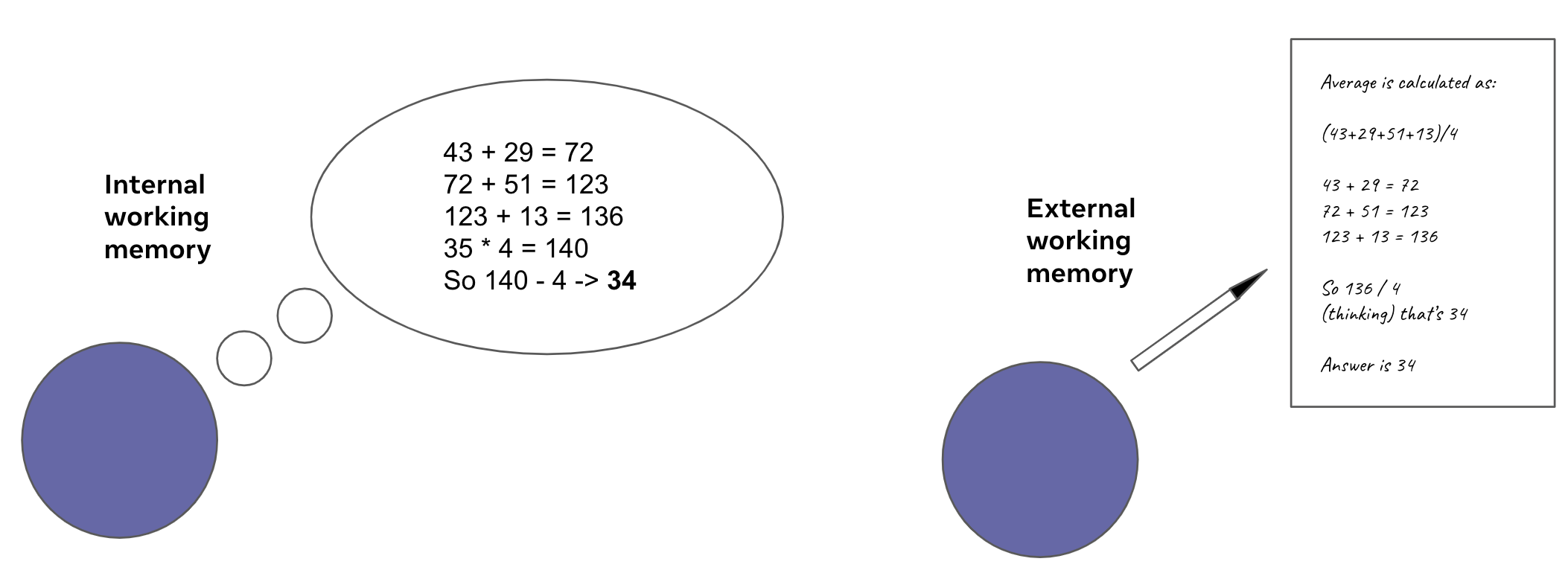
There are two limitations with chain-of-thought. First, it relies on prompt discovery to find a prompt that elicits robust step-by-step reasoning; i.e. minimizes mistakes from doing too much in a single forward pass. Not only does this require finding a robust prompt that works in all cases, but it also often relies on few-shot examples which take up context space. What is worse, much of the step-by-step reasoning on the internet misses intermediate steps that a human has performed using internal memory. Humans do not write down every step they perform because it would lead to long and tedious answers. They write down the principal steps of reasoning, and do lower-level steps via internal working memory. This means there is "missing data" in written text, i.e. between written steps there are internal memory steps that are not explicitly stated.

Secondly, chain-of-thought prompting uses the neural network to perform tasks that it is arguably not best suited to doing; for example, arithmetic. Prior work has shown that accuracy on tasks like multiplication is proportional to term frequency (Razeghi et al., 2022). Given that classical computers are specialized for tasks like arithmetic, one strategy is to offload these tasks from the neural network to external modules. For example, prior work has looked at the possibilities of external tool augmentation, such as calculators (Thoppilan et al., 2022). However, this requires a strategy to identify where the neural network should offload; and it may not be straightforward when combined with a discovered zero-shot prompt, especially where lower-level computation steps are not explicitly stated in writing.

Our solution is a working memory token we call <work>. We construct a few prompt datasets, see Table 3, that wrap step-by-by-step reasoning within <work> </work>. Some of these datasets were generated programmatically (OneSmallStep), by creating a problem template and sampling the variables, others were sourced online (Workout, Khan Problems), and others used existing datasets and transformed them into a <work> based context (GSM8k train). Where a computation is performed that a human could not do internally, we offload by writing and executing a Python script. An example is shown in Figure 3. Importantly, we do not have to turn this on, and the model can also predict the output from running a program. For our experiments, we did not find the need to turn Python offloading on, and leave this aspect to future work.

Figure 3: Model-Machine Symbiosis. We show an example answer with the <work> working memory token. It performs exact steps for rearranging the equation, and when it reaches a calculation that it cannot solve reliably in a forward-pass, it writes a program, which can then be offloaded to a classical computer.

Data source	Split	Prompts	Tokens
GSM8k (Cobbe et al., 2021)	train	7,473	3,518,467
OneSmallStep	n/a	9,314	3,392,252
Khan Problems (Hendrycks et al., 2021)	n/a	3,835	1,502,644
Workout	n/a	921	470,921
Total		21,543	9 million

Table 3: Reasoning Datasets To train the model to use <work> we include several datasets in pre-training that incorporate this token. Full details are contained in the Appendix.

Longer term, an architecture change may be needed to support adaptive computation, so machines can have internal working memory on the lines of work such as adaptive computation time and PonderNet (Graves, 2016; Banino et al., 2021). In this paper, we explore the <work> external working memory approach as a bridge to the next step. Notably our <work> prompt datasets are not very large or diverse, so there are likely large further gains to be made with this approach.

3.1.2 Citation Token

A distinctive properties of academic text is citations. In order to represent the implicit citation graph within the text, we process citations with global identifiers and special tokens [START_REF] and [END_REF] signifying when a citation is made. Figure 4 shows an example of citation processed text from a paper.

Figure 4: Citation Processed Text. Example of citation processed text from Attention Is All You Need (Vaswani et al., 2017). For title-processed citations, the title can be associated with the previous context.

We considered two type of citation identifier: (a) paper titles and (b) alphanumeric IDs. Based on ablations, we found that title based identifiers have greater citation prediction accuracy than IDs. However, we also found that paper titles are more prone to hallucination error at lower scales given the text-based nature of the identifier. We consider title processing for this paper, but we note the trade-offs between both approaches. Experiments for these ablations are contained in the Appendix.

3.2 Prompt Pre-Training

Figure 5: Prompt Pre-training. Pre-training weighs all tokens equally as part of the self-supervised loss. This leads to a weak relative signal for tasks of interest, meaning model scale has to be large to work. Instruction tuning boosts performance post hoc, and can generalize to unseen tasks of interest, but it risks performance in tasks that are distant from instruction set tasks. Prompt pre-training has a weaker task of interest bias than instruction tuning but less risk of degrading overall task generality.

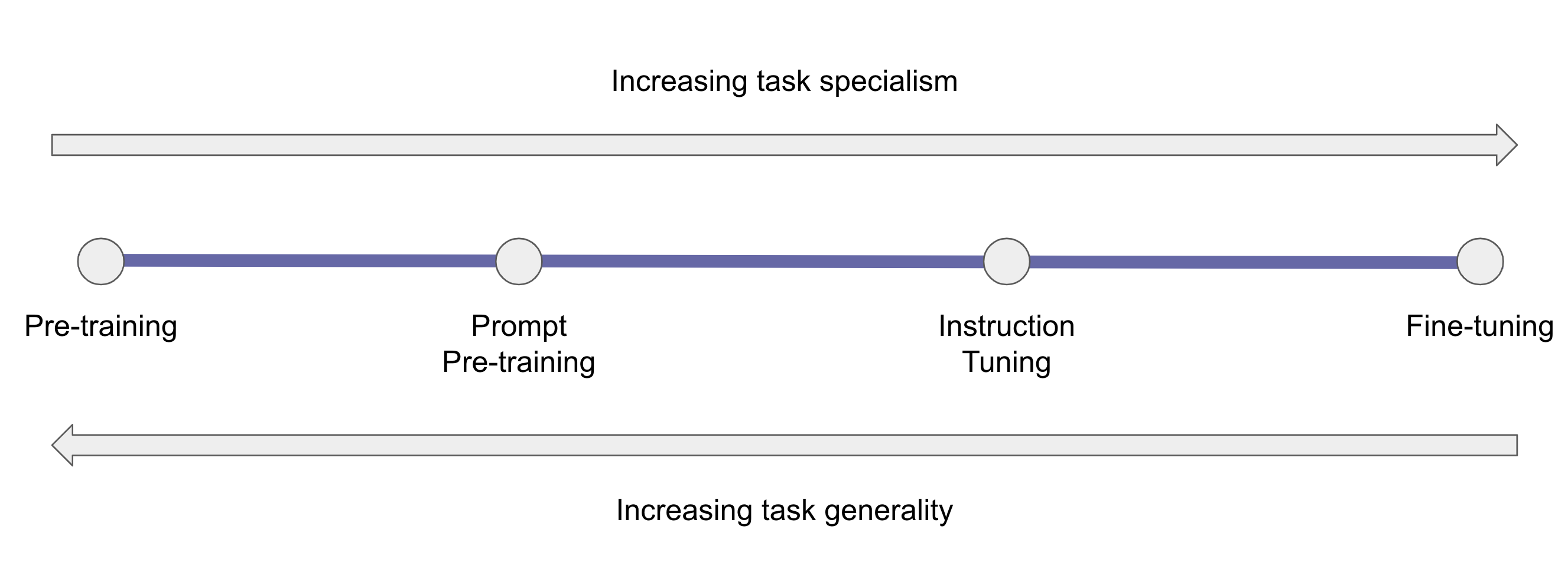
We deviate from existing language model research in one important direction, which is our decision to include prompts in pre-training alongside the general corpora. This is motivated by a number of observations.

First, existing work has shown the importance of training token count on performance. The Chinchilla paper derived scaling "laws" taking into account number of tokens, training a 70bn model for 1.4 trillion tokens (Hoffmann et al., 2022). They obtained state-of-the-art performance on MMLU, beating much larger models such as Gopher (Rae et al., 2021).

Separately, research such as FLAN and T0 showed prompt tuning can boost downstream performance (Wei et al., 2021; Sanh et al., 2021; Chung et al., 2022). Their strategy involved converting tasks to text prompts, using prompt diversity in how the tasks are posed, and then fine-tuning on these prompt datasets. For FLAN and T0, this approach boosts performance, beating larger models such as GPT-3 on many tasks.

And additionally there is the UnifiedQA approach (Khashabi et al., 2020). In this approach, a T5 model is fine-tuned on question answering datasets, and is shown to boost performance on out-of-domain question answering datasets (Raffel et al., 2020). The model outperforms GPT-3 on MMLU, a model 16 times larger.

The first stream of research above focuses on total training tokens as a way to boost performance; i.e. it is token agnostic. The second stream of research focuses on task-context tokens as a way to boost performance; i.e. it is token selective. Since fine-tuned smaller models beat larger few-shot models on tasks like MMLU, this suggests world knowledge may be present in smaller models, but task-context knowledge may be poor given the relative number of task-context tokens seen in the general corpus.

For this paper, we opt to augment pre-training data with more task prompts to boost performance at lower scales. This is advantageous if it obviates the need for more data scale, e.g. a >$1$ trillion corpus, or more model scale. The largest 120B model we train runs on a single NVIDIA A100 node. Additionally, given that fine-tuning requires expertise, making the model work out-the-box for popular tasks like question answering and summarization is more useful for users of the model. Lastly, by including prompts alongside general data, we maximize the generality of the model while boosting performance on some tasks of interest.

The closest analog to this approach for large language models is ExT5 (Aribandi et al., 2021). We take a similar approach by taking many machine learning training datasets, converting them to a text format, with prompt diversity, and then including them alongside general corpora in our pre-training set. A summary of prompt types is given in Table 4; the full details of datasets and prompts used are covered in the Appendix.

Task	Prompts	Tokens
Chemical Properties	782,599	275 million
Multiple-Choice QA	256,886	31 million
Extractive QA	30,935	13 million
Summarization	6,339	11 million
Entity Extraction	156,007	9 million
Reasoning	21,543	9 million
Dialog	18,930	5 million
Binary QA	36,334	4 million
Other	3,559	1 million
Total	783,599	358 million

Table 4: Pre-training Prompts. We include zero-shot prompts in pre-training to boost the task signal.

Because of prompt inclusion, it is important to distinguish between in-domain performance, where the training dataset is included in pre-training, and out-of-domain performance, where the training dataset is not included in pre-training. We mark these results clearly in the Results section of this paper. Importantly, we do not advocate for prompt pre-training as an alternative to instruction tuning. In fact, instruction tuning on Galactica is likely useful follow-up work given its potential to boost performance on several tasks of interest.

4 Method

4.1 Architecture

Galactica uses a Transformer architecture in a decoder-only setup (Vaswani et al., 2017), with the following modifications:

• GeLU Activation - we use GeLU activations for all model sizes (Hendrycks and Gimpel, 2016).

• Context Window - we use a 2048 length context window for all model sizes.

• No Biases - following PaLM, we do not use biases in any of the dense kernels or layer norms (Chowdhery et al., 2022).

• Learned Positional Embeddings - we use learned positional embeddings for the model. We experimented with ALiBi at smaller scales but did not observe large gains, so we did not use it (Press et al., 2021).

• Vocabulary - we construct a vocabulary of 50k tokens using BPE (Sennrich et al., 2015). The vocabulary was generated from a randomly selected 2% subset of the training data.

4.2 Models

The different model sizes we trained, along with training hyperparameters are outlined in Table 5.

Model	$n_{params}$	$n_{layers}$	$d_{model}$	$n_{heads}$	$d_{heads}$	Batch Size	Max LR	Warmup
GAL 125M	125M	12	768	12	64	0.5M	$6\times {10}^{-4}$	375M
GAL 1.3B	1.3B	24	2,048	32	64	1.0M	$2\times {10}^{-4}$	375M
GAL 6.7B	6.7B	32	4,096	32	128	2.0M	$1.2\times {10}^{-4}$	375M
GAL 30B	30.0B	48	7,168	56	128	2.0M	$1\times {10}^{-4}$	375M
GAL 120B	120.0B	96	10,240	80	128	2.0M	$0.7\times {10}^{-5}$	1.125B

Table 5: Details of the models trained

We train using AdamW with ${\beta }_1=0.9$, ${\beta }_2=0.95$ and weight decay of $0.1$ (Loshchilov and Hutter, 2017). We clip the global norm of the gradient at 1.0, and we use linear decay for learning rate down to 10% of it value. We use dropout and attention dropout of $p=0.1$. We do not use embedding dropout. We found longer warmup was important for the largest model in the early stages of training to protect against the effects of bad initialization, which can have long-memory effects on the optimizer variance state and slow down learning. This may be specific to our model and training setup, and it is not clear whether this advice generalizes.

4.3 Libraries and Infrastructure

We use the metaseq library for training the models, built by the NextSys team at Meta AI.

For training the largest 120B model, we use 128 NVIDIA A100 80GB nodes. For inference Galactica 120B requires a single A100 node. We choose the maximum model size to obey this constraint for downstream accessibility, and we will work to improve its accessibility for the research community in coming months.

5 Results

Figure 6: Repeated Tokens and Validation Loss. With four epochs of training, we continue to see validation loss fall for all model sizes. For the 120B model we see the first signs of overfitting at the beginning of the fifth epoch, and we early stop at this point.

5.1 Repeated Tokens Considered Not Harmful

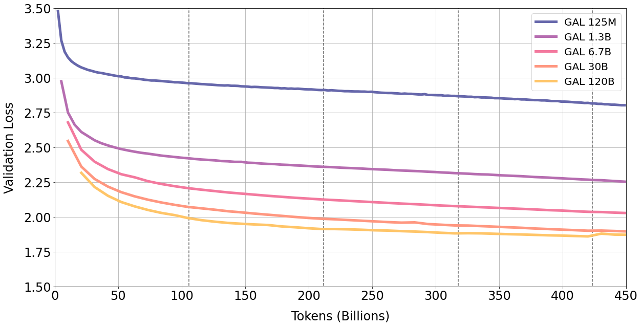
We train the models for 450 billion tokens, or approximately 4.25 epochs. We find that performance continues to improve on validation set, in-domain and out-of-domain benchmarks with multiple repeats of the corpus.

First, from Figure 6, validation loss continues to fall with four epochs of training. The largest 120B model only begins to overfit at the start of the fifth epoch. This is unexpected as existing research suggests repeated tokens can be harmful on performance (Hernandez et al., 2022). We also find the 30B and 120B exhibit a epoch-wise double descent effect of plateauing (or rising) validation loss followed by a decline. This effect becomes stronger with each epoch, and is most visible above with the 120B model towards end of training.

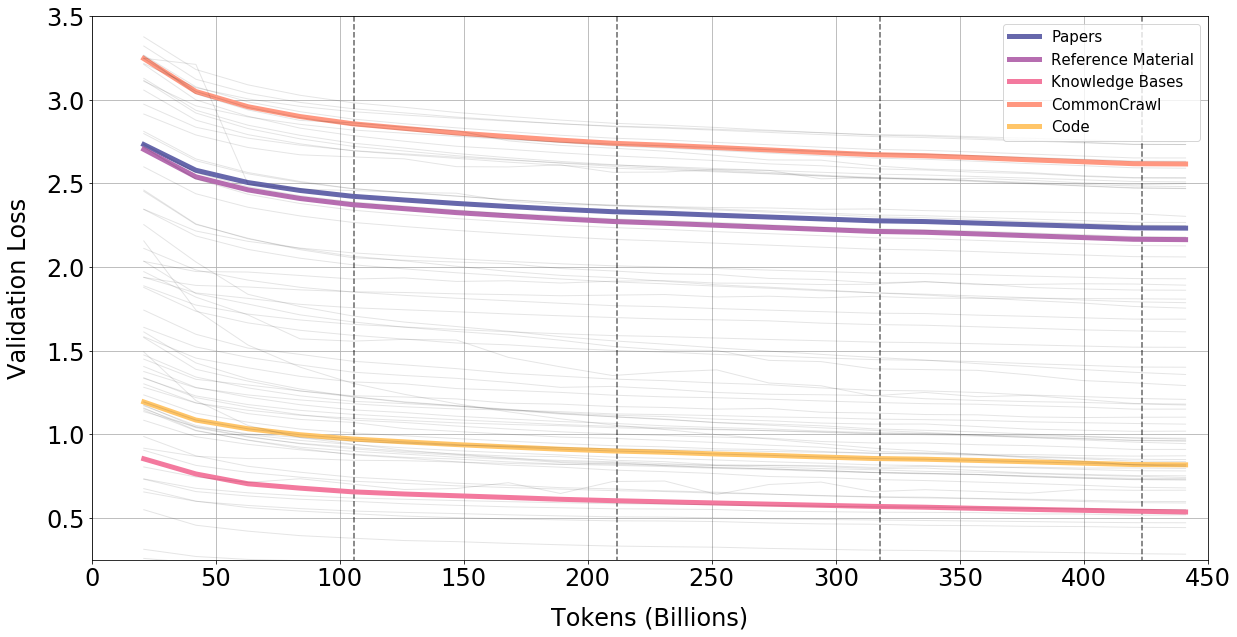
To investigate further, we examine the per-source breakdown of validation loss to see if there is heterogeneity in loss behaviour. We plot example curves in Figure 23 overleaf for the 30B model. We see no signs of loss heterogeneity: loss falls for all sources. The 120B exhibits the same relative trend of declining validation loss for all sources until the beginning of fifth epoch, where all sources spike (see Appendix).

Figure 7: Validation Loss Per Source. Validation loss falls through training for all dataset categories. Results are shown for the 30B model above. The 120B exhibits the same relative trend of declining validation loss for all sources until the beginning of fifth epoch, where all sources spike (see Appendix).

The next question to answer is whether this trend extends to downstream performance and out-of-domain generalization. For this we use a 57 task subset of BIG-bench subset, a general corpus with principally non-scientific tasks and prompt types not included in pre-training (Srivastava et al., 2022). We plot results in Figure 8. We see no signs of overfitting suggesting that use of repeated tokens is improving downstream performance as well as upstream performance.

Figure 8: BIG-bench Performance During Training. The 57 task selection from BIG-bench contains principally non-scientific tasks. We use it as a proxy for out-of-domain performance. For the 120B model above, we see no signs of overfitting after four repeats of the corpus.

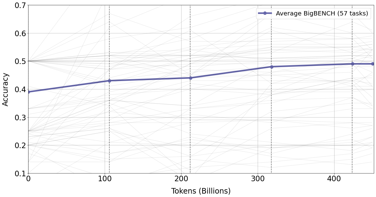
We suspect that two factors could be at play, a quality factor, the curated nature of the corpus enables more value per token to be extracted, or a modality factor, the nature of scientific data enables more value per token to be extracted. The missing step of causation is what leads specifically from either factor towards less overfitting, and we leave this question to further work. We note the implication that the "$\text{tokens}\to \mathrm{\infty }$" focus of current LLM projects may be overemphasised versus the importance of filtering the corpus for quality.

In the following sections, we turn to evaluating Galactica’s scientific capabilities. Specifically, we focus on the high-level design goals of building an LLM that can store, combine and reason about scientific knowledge - as these are needed for building a new interface for science.

5.2 Knowledge Probes

First, we examine how well Galactica absorbs scientific knowledge. We set up several knowledge probe benchmarks, building off the LAMA approach of Petroni et al. (2019). These were critical metrics during model development for identifying knowledge gaps within the corpus, and informing how to iterate the corpus. They also provide insight into the relative knowledge strengths of Galactica versus general language models, and we cover these results in this section before turning to the downstream tasks.

5.2.1 LaTeX Equations

We construct a dataset of popular LaTeX equations from the fields of chemistry, physics, mathematics, statistics and economics. Memorisation of equations is useful to measure as it is necessary for many downstream tasks; for example, recalling an equation to use as part of an answer to a problem. Unless stated explicitly, Galactica results are reported as zero-shot. In total there are 434 equations we test for the knowledge probe.

We prompt with an equation name and generate LaTeX. An example is shown in Figure 9.

Figure 9: LaTeX Equations Probe. We prompt for the name of an equation and evaluate whether the generated LaTeX is correct. We manually evaluate given the possibility of multiple correct answers.

We summarize the results in Table 6. Equation knowledge increases smoothly with scale. Galactica outperforms larger language models trained on general corpuses, indicating the value of a curated dataset.

Model	Params (bn)	Chemistry	Maths	Physics	Stats	Econ	Overall
OPT	175	34.1%	4.5%	22.9%	1.0%	2.3%	8.9%
BLOOM	176	36.3%	36.1%	6.6%	14.1%	13.6%	21.4%
GPT-3 (text-davinci-002)	?	61.4%	65.4%	41.9%	25.3%	31.8%	49.0%
GAL 125M	0.1	0.0%	0.8%	0.0%	1.0%	0.0%	0.5%
GAL 1.3B	1.3	31.8%	26.3%	23.8%	11.1%	4.6%	20.5%
GAL 6.7B	6.7	43.2%	59.4%	36.2%	29.3%	27.3%	41.7%
GAL 30B	30	63.6%	74.4%	35.2%	40.4%	34.1%	51.5%
GAL 120B	120	79.6%	83.5%	72.4%	52.5%	36.4%	68.2%

Table 6: Results on LaTeX equations. Results are evaluated zero-shot.

5.2.2 Domain Probes

We also set up domain probes to track specialized knowledge for certain fields. We detail these below:

• AminoProbe: a dataset of names, structures and properties of the 20 common amino acids.

• BioLAMA: a dataset of biomedical factual knowledge triples.

• Chemical Reactions: a dataset of chemical reactions.

• Galaxy Clusters: a dataset of galaxy clusters with their constellation classifications.

• Mineral Groups: a dataset of minerals and their mineral group classifications.

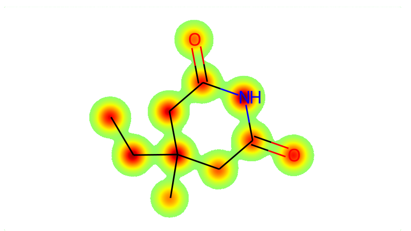
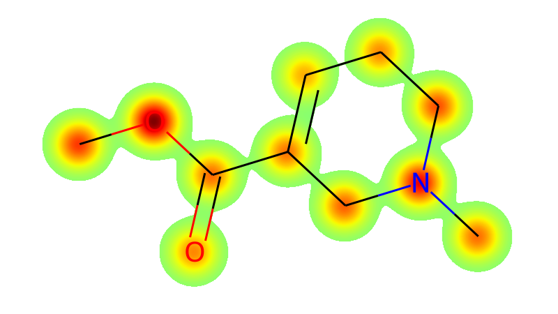
In each case, we construct a prompt to test the knowledge. For example, for Chemical Reactions, we ask Galactica to predict the products of the reaction in the chemical equation LaTeX. We mask out products in the description so the model is inferring based on the reactants only. An example is shown in Figure 10.

Figure 10: Chemical Reactions. We prompt based on a description and reactants, and evaluate whether the generated products are correct.

We report results for these knowledge probes in Table 7.

Model	Params (bn)	Amino	BioLAMA	Reactions	Clusters	Minerals
OPT	175	12.0%	7.1%	12.7%	21.7%	1.6%
BLOOM	176	14.0%	9.7%	22.4%	15.0%	10.3%
GPT-3 (text-davinci-002)	?	14.0%	8.4%	35.1%	20.8%	18.3%
GAL 125M	0.1	12.0%	3.1%	0.3%	6.7%	0.0%
GAL 1.3B	1.3	16.0%	7.2%	14.4%	14.2%	10.3%
GAL 6.7B	6.7	17.0%	7.9%	26.4%	17.5%	8.7%
GAL 30B	30	21.0%	6.9%	36.5%	20.0%	17.5%
GAL 120B	120	21.0%	8.0%	43.1%	24.2%	29.4%

Table 7: Results on Domain Probes. Results are evaluated zero-shot.

We also observe steady scaling behaviour in these knowledge probes, with the exception of BioLAMA which we suspect reflects zero-shot prompt difficulty for all LLMs. Notably fine-grained factual knowledge, such as "ConstellationOf(GalaxyCluster)" type-queries seems to scale smoothly with the size of the model.

5.2.3 Reasoning

We now turn to reasoning capabilities with the <work> token. We start by evaluating on the MMLU mathematics benchmarks, which we report in Table 8 (Hendrycks et al., 2020). Galactica performs strongly compared to larger base models, and use of the <work> token appears to boost performance over Chinchilla, even for the smaller 30B Galactica model.

Mathematics MMLU
Model	Params (bn)	A.Algebra	Elem	HS	College	F. Logic	Average
BLOOM (5-shot)	176	25.0%	26.7%	27.0%	25.0%	26.2%	26.4%
OPT (5-shot)	175	21.0%	25.7%	24.4%	33.0%	29.4%	26.7%
Gopher (5-shot)	280	25.0%	33.6%	23.7%	37.0%	35.7%	30.6%
Chinchilla (5-shot)	70	31.0%	41.5%	31.9%	32.0%	33.3%	35.7%
GAL 1.3B	1.3	28.0%	27.2%	26.7%	30.0%	24.6%	27.1%
GAL 6.7B	6.7	28.0%	28.9%	26.7%	36.0%	31.0%	29.2%
GAL 30B	30	30.0%	30.2%	26.3%	36.0%	31.7%	29.9%
GAL 120B	120	33.0%	38.1%	32.6%	43.0%	32.5%	35.8%
GAL 1.3B <work>	1.3	22.0%	24.6%	18.9%	25.0%	31.0%	24.6%
GAL 6.7B <work>	6.7	33.3%	30.7%	25.2%	26.0%	33.3%	28.0%
GAL 30B <work>	30	33.0%	41.5%	33.3%	39.0%	37.3%	37.1%
GAL 120B <work>	120	27.0%	54.2%	37.0%	44.0%	40.5%	41.3%

Table 8: Results on Mathematics MMLU. Galactica is evaluated without few-shot examples. With the <work> token we see large gains in performance. Results are on MMLU test.

We also evaluate on the MATH dataset to further probe the reasoning capabilities of Galactica (Hendrycks et al., 2021). We compare the <work> token prompt directly with the Minerva 5-shot chain-of-thought prompt mCoT for comparability. We report results in Table 9.

MATH Results
Model	Alg	CProb	Geom	I.Alg	N.Theory	Prealg	Precalc	Average
Base Models
GPT-3 175B (8-shot)	6.0%	4.7%	3.1%	4.4%	4.4%	7.7%	4.0%	5.2%
PaLM 540B (5-shot) mCoT	9.7%	8.4%	7.3%	3.5%	6.0%	19.2%	4.4%	8.8%
GAL 30B <work>	15.8%	6.3%	5.8%	4.9%	2.4%	19.4%	8.2%	11.4%
GAL 30B (5-shot) mCoT	17.9%	6.8%	7.9%	7.0%	5.7%	17.9%	7.9%	12.7%
GAL 120B <work>	23.1%	10.1%	9.8%	8.6%	6.5%	23.8%	11.7%	16.6%
GAL 120B (5-shot) mCoT	29.0%	13.9%	12.3%	9.6%	11.7%	27.2%	12.8%	20.4%
Fine-tuned LaTeX Models
Minerva 540B (5-shot) mCoT	51.3%	28.0%	26.8%	13.7%	21.2%	55.0%	18.0%	33.6%

Table 9: Results on MATH. With both the chain-of-thought and <work> token prompts, Galactica exceeds PaLM’s performance with 18 times less capacity.

We see that Galactica outperforms the base PaLM model by a significant margin, with both chain-of-thought and <work> prompts. Galactica 30B outperforms PaLM 540B on both prompts: an 18 times smaller model. This suggests Galactica may be a better base model for fine-tuning towards mathematical tasks.

We report Minerva results for completeness, which is a 540B PaLM fine-tuned towards LaTeX specifically. Minerva outperforms base Galactica, but the performance differences are non-uniform; which points towards different mathematical data biases. For a direct comparison to Minerva, the model is freely available for those who want to finetune Galactica towards LaTeX specifically as follow-up work.

5.3 Downstream Scientific NLP

We now evaluate on downstream scientific tasks to see how well Galactica can compose its knowledge in different task contexts. We focus on knowledge-intensive scientific tasks and report full results in Table 10. For this we use the MMLU benchmark as well as some other popular scientific QA benchmarks. We include the MMLU results earlier without <work> to test for knowledge association specifically. Full MMLU results, including social sciences and other fields, are reported in the Appendix. We also perform data leakage analysis on these benchmarks for more confidence; results are in the Appendix.

From Table 10, Galactica can compose its knowledge into the question-answering task, and performance is strong; significantly outperforming the other open language models, and outperforming a larger model (Gopher 280B) in the majority of tasks. Performance against Chinchilla is more variable, and Chinchilla appears to be stronger in a subset of tasks: in particular, high-school subjects and less-mathematical, more memorization intensive tasks. In contrast, Galactica tends to perform better in mathematical and graduate-level tasks.

Our working hypothesis is that the Galactica corpus is biased towards graduate scientific knowledge, given it consists mostly of papers, which explains lagging performance in high-school subjects. While we do pick up some high-school level content through encyclopedias, textbooks and the filtered CommonCrawl, this amounts to a small quantity of tokens (a few billion). We leave the question of how to capture more of this base scientific knowledge in a curated way to future work.

On remaining tasks, we achieve state-of-the-art results over fine-tuned models at the time of writing. On PubMedQA, we achieve a score of 77.6% which outperforms the state-of-the-art of 72.2% (Yasunaga et al., 2022). On MedMCQA dev we achieve score of 52.9% versus the state-of-the-art of 41.0% (Gu et al., 2020). For BioASQ and MedQA-USMLE, performance is close to the state-of-the-art performance of fine-tuned models (94.8% and 44.6%) (Yasunaga et al., 2022).

Dataset	Domain	GAL	OPT	BLOOM	GPT-3	Gopher	Chinchilla
Abstract Algebra	out-of-domain	33.3%	21.0%	25.0%	-	25.0%	31.0%
ARC Challenge	in-domain	67.9%	31.1%	32.9%	51.4%	-	-
ARC Easy	in-domain	83.8%	37.4%	40.7%	68.8%	-	-
Astronomy	out-of-domain	65.1%	23.0%	25.7%	-	65.8%	73.0%
BioASQ	in-domain	94.3%	81.4%	91.4%	-	-	-
Biology (College)	out-of-domain	68.8%	30.6%	28.5%	-	70.8%	79.9%
Biology (High-School)	out-of-domain	69.4%	27.7%	29.4%	-	71.3%	80.3%
Chemistry (College)	out-of-domain	46.0%	30.0%	19.0%	-	45.0%	51.0%
Chemistry (High-School)	out-of-domain	47.8%	21.7%	23.2%	-	47.8%	58.1%
Comp. Science (College)	out-of-domain	49.0%	17.0%	6.0%	-	49.0%	51.0%
Comp. Science (High-School)	out-of-domain	70.0%	30.0%	25.0%	-	54.0%	58.0%
Econometrics	out-of-domain	42.1%	21.0%	23.7%	-	43.0%	38.6%
Electrical Engineering	out-of-domain	62.8%	36.6%	32.4%	-	60.0%	62.1%
Elementary Mathematics	out-of-domain	38.1%	25.7%	27.6%	-	33.6%	41.5%
Formal Logic	out-of-domain	32.5%	29.4%	26.2%	-	35.7%	33.3%
Machine Learning	out-of-domain	38.4%	28.6%	25.0%	-	41.1%	41.1%
Mathematics (College)	out-of-domain	43.0%	33.0%	25.0%	-	37.0%	32.0%
Mathematics (High-School)	out-of-domain	32.6%	24.4%	27.0%	-	23.7%	31.9%
Medical Genetics	out-of-domain	70.0%	35.0%	36.0%	-	69.0%	69.0%
Physics (College)	out-of-domain	42.2%	21.6%	18.6%	-	34.3%	46.1%
Physics (High-School)	out-of-domain	33.8%	29.8%	25.2%	-	33.8%	36.4%
MedQA-USMLE	out-of-domain	44.4%	22.8%	23.3%	-	-	-
MedMCQA Dev	in-domain	52.9%	29.6%	32.5%	-	-	-
PubMedQA	in-domain	77.6%	70.2%	73.6%	-	-	-
Statistics (High-School)	out-of-domain	41.2%	43.5%	19.4%	-	50.0%	58.8%

Table 10: Question Answering Results. Galactica is evaluated without few-shot examples. Other LLMs are evaluated 5-shot, except for 0-shot results for GPT-3 on ARC results and OPT and BLOOM on PubMedQA and BioASQ. For abstract algebra and medical genetics, we obtained best results with 30B, so we report these scores; the 120B scores for these were 27.0% and 68.0% respectively. Rest of results are for 120B.

5.4 Citation Prediction

In this section we evaluate Galactica’s capability to predict citations given an input context, which is an important test of Galactica’s capability to organize the scientific literature. We find that both accuracy and the quality of distributional approximation improves with scale.

5.4.1 Citation Accuracy

We construct three datasets to evaluate the model’s capability to cite:

• PWC Citations: a dataset with 644 pairs of machine learning concepts and papers that introduced them. Concepts consist of methods (e.g. ResNet) and datasets (e.g. ImageNet) from Papers with Code.

• Extended Citations: a dataset with 110 pairs of non-machine learning concepts and papers that introduced them. Examples of concepts include Kozac sequence and Breit-Wigner distribution.

• Contextual Citations: a dataset with 1,869 pairs of references and contexts from our arXiv validation set. The dataset is constructed by sampling 1,000 random references and collecting their contexts.

For the PWC Citations and Extended Citations datasets, the citation prediction task is framed as a text generation task. The model is given a prompt like "In this paper we use ResNet method [START_REF]" in order to generate a prediction for the ResNet concept. For Contextual Citations, we prompt after the input context for the citation, where the context ends with [START_REF].

We compare Galactica to sparse and dense retrieval-based approaches on this task.

For the sparse baseline, we use ElasticSearch to create an index of all the references, including their titles, abstracts, and short snippets of text with the contexts they appear in. Then, given a text query, we retrieve the top references ordered by the sum of matching scores across all selected fields.

For dense retriever baselines, we evaluate two different Contriever models (Izacard et al., 2021). The first is the pre-trained model released by Izacard et al. (2021). The second model we use is fine-tuned on a random subset of 10 million context/paper pairs from our corpus, trained to retrieve the right paper given a context before a citation. The setup for dense retrieval is: (1) each reference is encoded by the model using its title and abstract, (2) a text query is encoded by the same model, (3) the references that match the query re returned. Retrieval is performed using a FAISS index (Johnson et al., 2019).

The results can be seen in Table 11.

Model	Params (bn)	PWC Citations	Extended Citations	Contextual Citations
GAL 125M	0.1	7.0%	6.4%	7.1%
GAL 1.3B	1.3	18.5%	45.5%	15.9%
GAL 6.7B	6.7	32.0%	60.0%	23.0%
GAL 30B	30	44.7%	66.4%	31.5%
GAL 120B	120	51.9%	69.1%	36.6%
Sparse Retriever	n/a	30.9%	17.3%	5.3%
Dense Retriever (base)	n/a	16.4%	8.8%	1.6%
Dense Retriever (fine-tuned)	n/a	27.6%	11.8%	8.2%

Table 11: Citation Prediction Accuracy. Performance of different model sizes on citation prediction.

The performance on all evaluation sets increases smoothly with scale. At larger scales, Galactica outperforms the retrieval-based approaches as its context-associative power improves. This is an important result as current approaches for navigating the literature use these existing retrieval approaches. As the power of language models improves, we suspect they will become a valuable new tool for exploring the literature.

5.4.2 Citation Distributional Analysis

(a) Kolmogorov-Smirnov Distance

(b) Histogram Overlap

Figure 11: Distributional Comparison of Citations. Galactica’s citation distribution approaches the ground truth with scale. This is seen through a declining KS distance with scale, and increasing histogram overlap.

We now turn to look at how well Galactica can model the empirical citation distribution. For this analysis we use the Contextual Citations dataset, where prompts are extracted from a paper by taking the context before a citation as the prompt. An example prompt with a model prediction is shown overleaf in Figure 12.

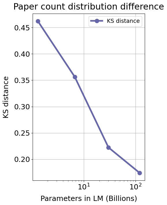
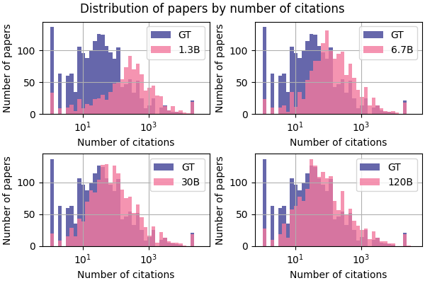
We use the in-context citation data to analyse the distributional difference between predicted and ground truth paper counts. This allows us to assess the model bias towards predicting more popular papers. Specifically, for each context there is a ground truth and predicted reference. We count the number of times each reference appears in our corpus. We then compare the distribution of reference counts between the ground truth references and the predicted references using the Kolmogorov-Smirnov distance (Massey, 1951).

The comparison between the citation count distributions for different model sizes can be seen in Figure 11. Figure 11(a) shows the decrease in the Kolmogorov-Smirnov distance between the distribution of ground truth paper citations and the distribution of predicted papers citations. Figure 11(b) shows how the distribution of paper counts for the predicted papers gets closer to the ground truth as the model size grows. At smaller scales the model is more prone to predicting more popular papers. As the model grows in size this bias towards predicting popular papers diminishes.

Figure 12: Citation Prompt. An example prompt predicting a citation in-context; from Briol et al. (2015).

5.5 General Capabilities

We have studied Galactica’s scientific capabilities. It is perhaps not surprising that a specialist scientific model outperforms general models on scientific tasks, but what would be more surprising was if it outperformed general models on general NLP tasks. In this section, we show surprising evidence that it does just that.

We evaluate on 57 BIG-bench tasks in Table 12 (Srivastava et al., 2022). The tasks are primarily non-scientific and test general language capability, for example anachronisms, figure of speech and metaphor boolean. We always evaluate with 5-shots, and we use the default prompt style from BIG-Bench. Importantly, we do not include this prompt style in pre-training; so the evaluation between Galactica and the other models is comparable 5-shot. Full details and results are in the Appendix. We summarize average scores in Table 12:

Model	Params (bn)	Accuracy	Accuracy
		weighted	unweighted
OPT 30B	30	39.6%	38.0%
BLOOM 176B	176	42.6%	42.2%
OPT 175B	175	43.4%	42.6%
GAL 30B	30	46.6%	42.7%
GAL 120B	120	48.7%	45.3%

Table 12: BIG-bench 57 Task Results. Galactica outperforms general open models at smaller scales.

Both the 30B and 120B Galactica models outperform the larger OPT and BLOOM general models. This is a surprising result given we designed Galactica to trade-off generality for performance in scientific tasks.

We suspect this result reflects the higher-quality of the Galactica corpus, stemming from the fact it is curated and also primarily academic text. Previous open LLM efforts likely overfocused on scale goals and underfocused on data filtering. Another implication is that the focus on tokens $\to \mathrm{\infty }$ from Chinchilla needs to be complemented with strong data quality procedures (Hoffmann et al., 2022). With this paper, we took an opposite approach by focusing on high-quality tokens and repeated epochs of training. However, the Chinchilla insight stands: and there is much more scientific text that we have not exploited in this work.

5.6 Chemical Understanding

We now turn to Galactica’s capability to interface with different scientific modalities. We start by looking at Galactica’s chemical capabilities. Chemical properties exhibit complex correlations which means the chemical space is very large. Better organization of chemical information through language models could aid chemical design and discovery. We explore how Galactica can provide a new interface for these tasks in this section.

For this work, we only include a small subset of available compounds from PubChem Compound in pre-training. Specifically, we take a random subset ($2$ million) of total compounds ($110$ million). This is to ensure the model is not overly biased towards learning natural sequences over natural language. This is a constraint we can relax in future work, enabling for much larger corpus. Here we focus on the first step of investigating whether a single model can learn effectively in the multi-modal setting.

We find that a language model can learn chemical tasks such as IUPAC naming in a self-supervised way, and in addition, we can pose drug discovery tasks as natural language prompts and achieve reasonable results.

5.6.1 IUPAC Name Prediction

SMILES is a line notation which represents chemical structure as a sequence of characters (Weininger, 1988). In the Galactica corpus, the SMILES formula occurs alongside information in the document, such as IUPAC names, molecular weight and XLogP. In the context of self-supervised learning, this means a language model is performing implicit multi-task learning: the model is predicting the next SMILES token, but can also use SMILES to predict other entities in the document.

As an initial test, we set up a IUPAC Name Prediction task, where the task is to name a compound according to the IUPAC nomenclature given a SMILES formula input. The IUPAC nomenclature is a method of naming organic compounds that has a ruleset based on naming the longest chain of carbons connected by single bonds (Favre and Powerll, ). There is a large set of rules and the procedure is algorithmically complex, meaning it is hard to automate. As a result, it is missing from standard cheminformatics toolkits.

Previous works such as STOUT and Struct2IUPAC have explored the possiblity of using RNNs and Transformers for this task (Rajan et al., 2021; Krasnov et al., 2021). We explore in this section whether Galactica can translate a SMILES specification to its IUPAC name in the self-supervised setting. We design a prompt based on the PubChem structure, with the SMILES as the only input, and the output to predict the IUPAC name.

To evaluate, we use our compound validation set of 17,052 compounds, and prompt with the SMILES formula and predict the IUPAC name. To calculate accuracy, we use OPSIN to convert the generated IUPAC name to SMILES, canonicalize it and compare with the canonicalized SMILES target (Lowe et al., 2011).

Results are shown in Table 13.

Model	Params (bn)	Accuracy	Invalid Names
GAL 125M	0.1	0.0%	32.8%
GAL 1.3B	1.3	2.5%	12.0%
GAL 6.7B	6.7	10.7%	12.3%
GAL 30B	30	15.4%	9.7%
GAL 120B	120	39.2%	9.2%

Table 13: Results on IUPAC Naming. Performance improves smoothly with scale.

Accuracy increases smoothly with scale. Given we restricted the corpus to 2 million molecules, it is likely much better performance is achievable through training or fine-tuning on more molecules. The model is freely available for those who want to perform this follow-up work.

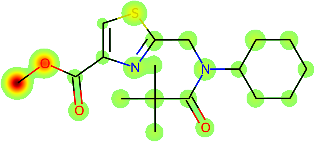
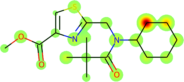
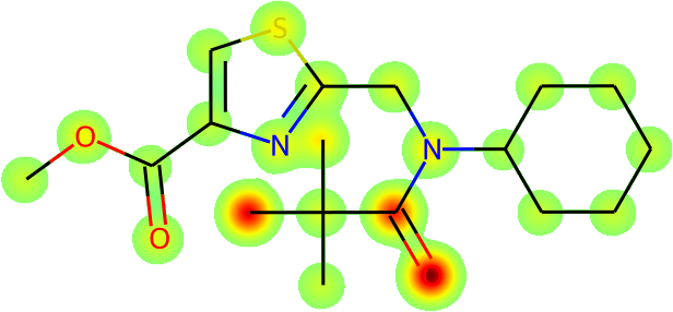
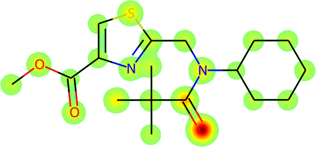
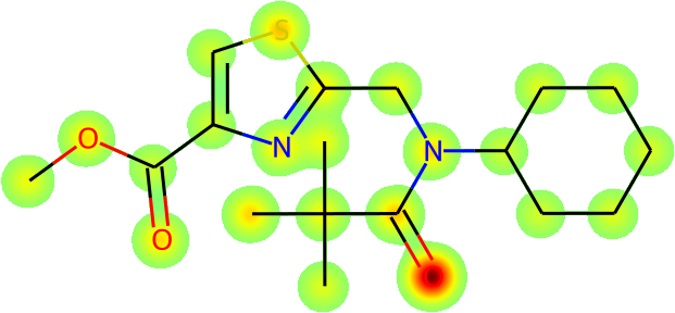
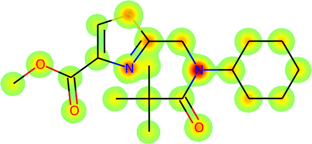
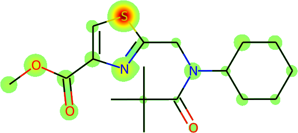
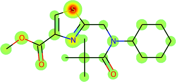
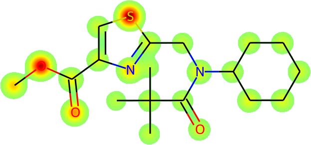
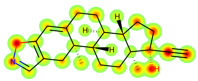
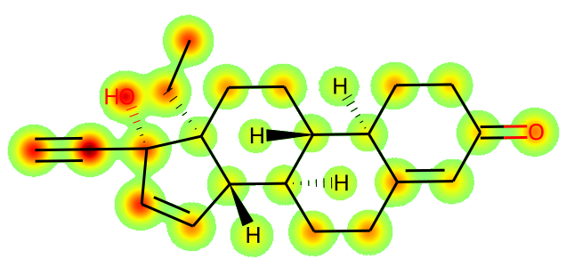
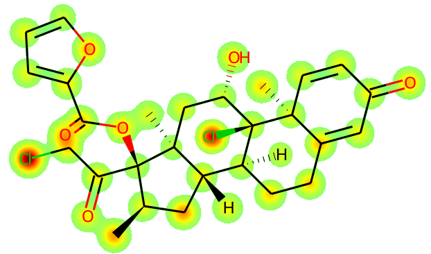
The more immediate question is what is actually being learnt: is Galactica inferring names from the fundamental molecular structure? To answer this, we visualize the average atomic attention at each stage of a prediction in Figure 13 overleaf. Encouragingly, the results are interpretable in terms of the underlying chemistry, and Galactica attends to the correct group when predicting a name, e.g. for "amino" it attends primarily to the $-N{H}_2$ substituent.

Task: Convert the SMILES to IUPAC Name
Example: CC(C)(C)C(=O)N(CC1=NC(=CS1)C(=O)OC)C2CCCCC2

Atomic Attention	Predicted So Far	Token Predicted
	-	methyl
	methyl 2-[[cyclohexyl	cyclohexyl
	methyl 2-[[cyclohexyl-(2,2-	dimethyl
	methyl 2-[[cyclohexyl-(2,2-dimethyl	prop
	methyl 2-[[cyclohexyl-(2,2-dimethylprop	anoyl
	methyl 2-[[cyclohexyl-(2,2-dimethylpropanoyl)	amino
	methyl 2-[[cyclohexyl-(2,2-dimethylpropanoyl)]amino] methyl]	th
	methyl 2-[[cyclohexyl-(2,2-dimethylpropanoyl)]amino] methyl]th	iazole
	methyl 2-[[cyclohexyl-(2,2-dimethylpropanoyl)]amino] methyl]thiazole-4-	carboxylate

Figure 13: Attending to Functional Groups. Galactica uses its knowledge of chemistry to help with the IUPAC Naming task. At each stage of prediction, it attends to the part of the molecular graph associated with the group name, e.g. for "amino" it attends to the nitrogen atom; for thiazole, the sulphur atom.

5.6.2 MoleculeNet

We now explore whether we can pose traditional drug discovery tasks in a natural language format, combining the different modalities involved. Humans organize knowledge via natural language, and so learning an interface between natural language and scientific modalities like SMILES could be a new tool for navigating the chemical space. We use MoleculeNet classification benchmarks to answer this question, which are summarized in Table 14 (Wu et al., 2017).

Category	Dataset	Type	Other modalities
Biophysics	HIV	Classification	n/a
	BACE C	Classification	n/a
Physiology	BBBP	Classification	n/a
	Tox21	Classification	protein sequences
	SIDER	Classification	n/a
	ClinTox	Classification	n/a

Table 14: MoleculeNet datasets used for evaluation. We convert training sets to text format and include in pre-training. We evaluate using the splits suggested by the DeepChem library (Ramsundar et al., 2019).

To evaluate, we include the training sets in pre-training by converting to a text format. We use prompt randomization (varying how the question is posed). For example, for BBBP the training prompt has forms like in Figure 14 below. These examples occur alongside the other corpuses in training, and each example is seen just over $4$ times. This is not comparable to direct fine-tuning or supervision due to the presence of other data in pre-training, so it might be considered a form of weak supervision instead.

Figure 14: BBBP Prompt. We include the SMILES and pose the classification problem in natural language.

For some MoleculeNet datasets, other modalities are implicitly present. For example, in the Tox21 dataset, bioassays concern particular receptors such as the androgen receptor (AR). As an experiment, we decided to frame the task in a text format with the protein sequence and the SMILES as part of the prompt. We show an example for Tox21 in Figure 15.

Figure 15: Tox21 Prompt. We include the protein sequence and the SMILES formula and pose the classification problem in natural language.

We make sure to Kekulize the SMILES to be consistent with PubChem representations. For evaluation, we use the recommended splits from the DeepChem library (Ramsundar et al., 2019).

We present results in Table 15. Performance scales with model size. The scaling is slower than tasks like QA, and the base model lags a specialist model with explicit 3D information and 10 times more molecules (Zhou et al., 2022). We suspect the weak supervision setup is harder for this task, and fine-tuning and/or more molecule data is required to get sufficient task signal. The model is available for work on this.

MoleculeNet Classification
Model	Modality	Molecules	BACE	BBBP	ClinTox	HIV	SIDER	Tox21	Av.
GAL 125M	SMILES	2M	0.561	0.393	0.518	0.702	0.559	0.543	0.581
GAL 1.3B	SMILES	2M	0.576	0.604	0.589	0.724	0.540	0.606	0.619
GAL 6.7B	SMILES	2M	0.584	0.535	0.784	0.722	0.559	0.639	0.640
GAL 30B	SMILES	2M	0.727	0.596	0.822	0.759	0.613	0.685	0.687
GAL 120B	SMILES	2M	0.617	0.661	0.826	0.745	0.632	0.689	0.690
Uni-Mol	3D	20M	0.857	0.729	0.919	0.808	0.659	0.796	0.770

Table 15: Results on MoleculeNet Classification. Results are scored by ROC-AUC.

For our purposes, the implication for future work is that we can learn drug discovery tasks via natural language prompts. If we can learn these relationships automatically in a signal-dense document context (e.g. online chemical databases), this might reduce the reliance on supervised datasets to perform these tasks.

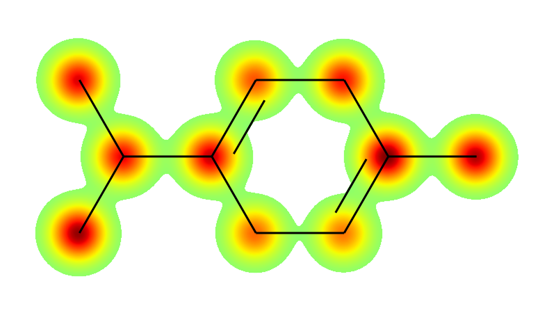
As a final check, we can average Galactica’s attention heads across layers, and visualize whereabouts the model looks in the SMILES sequence to make a prediction (atomic attention). We show an example in Figure 16 for some Tox21 predictions.

Positive Examples

(a) Danazol (28417) on NR-AR

(b) Gestodene (3033968) on NR-AR

(c) Mometasone f. (441336) on NR-AR

Negative Examples

(d) $\gamma$-Terpinene (7461) on NR-PPAR-$\gamma$

(e) Bemegride (2310) on NR-AR

(f) Arecoline (2230) on NR-PPAR-$\gamma$

Figure 16: Attention Visualization on Tox21. The top three molecules are highest confidence positive examples for the 30B model; the bottom three are the highest confidence negatives. We match attention weights from the SMILES with the canonical atom ordering. Danazol and gestodene are known to possess high affinities for the androgen receptor (AR) (Nieschlag et al., 2010).

5.7 Biological Understanding

In this section we examine Galactica’s capability to interface with biological modalities. Language models could potentially play a role in automatic organisation of this data, for example annotating newly sequenced proteins with functional information. We explore the potential of this interface in this section.

For protein sequences from UniProt, we include a small subset of available sequences in pre-training. Specifically, we take reviewed Swiss-Prot proteins; a high-quality subset ($0.5$ million) of total ($227$ million). This is to ensure the model is not overly biased towards learning natural sequences over natural language. As with molecule data, this is a constraint we can relax in future work, enabling for much larger corpus. Here we focus on the first step of investigating whether a single model can learn effectively in the multi-modal setting.

We find that a language model can learn an implicit measure of sequence similarity that it can use for tasks such as functional annotation and descriptions.

5.7.1 Sequence Validation Perplexity

Figure 17: Primary Structure Prediction. For three of the validation sets we observe smooth scaling, reflecting the potential for high sequence similarity with sequences in the training set; for example, orthologs in the case of the Paen validation set. The CASP set with sequence similarity constraints levels off, suggesting the gains from the 550k proteins in training quickly saturates for more out-of-domain sequences.

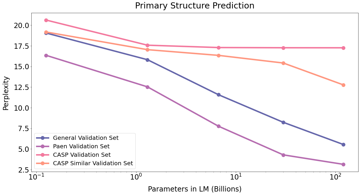
While Galactica does not explicitly model the 3D structure of a protein, the information needed for a specific conformation is contained in the linear amino acid sequence, which in turn determine function. As a first step, we test upstream performance through evaluating protein sequence perplexity. Constructing a good validation set is important and data leakage is a problem for works in this field. We construct four holdout sets to obtain more confidence about what is being learnt and what generalizes.

First, we conduct BLAST on the sequences in the training set and remove all sequences with a sequence identity $\ge 50\%$ with 51 CASP14 target sequences. These are the same test sequences used in ESMFold (Lin et al., 2022b). In total we remove 167 sequences from the training set using this approach. We call this this holdout set CASPSimilarSeq. We call the 51 CASP14 target sequences CASPSeq.

Secondly, we conduct organism-level holdout, and remove all sequences from the Paenungulata clade of organisms, including elephants, elephant shrews, manatees and aadvarks. This allows us to test whether Galactica can annotate sequeces for organisms it has never seen before. In total we remove 109 sequences from the training set using this approach. We call this holdout set PaenSeq. Note that this does not enforce any sequence similarity constraints, and there may be very similar sequences in the training set.

Lastly, we conduct a randomized test split, consisting of 5456 sequences. There is no sequence identity constraint applied, so memorization may be more at play, but it still provides a signal about the breadth of sequence knowledge absorbed by the model. We call this holdout set UniProtSeq.

We evaluate perplexity for all holdout sets in Table 16 and plot in Figure 17. For three of the validation sets we observe smooth scaling, reflecting the potential for high sequence similarity with sequences in the training set; for example, orthologs in the case of the Paen validation set. Interestingly, the CASP set with sequence similarity constraints levels off, suggesting the gains from the 550k proteins in training quickly saturates.

Protein Sequence Validation Perplexity
Model	Param (bn)	CASPSeq	CASPSimSeq	PaenSeq	UniProtSeq
GAL 125M	0.1	20.62	19.18	16.35	19.05
GAL 1.3B	1.3	17.58	17.04	12.53	15.82
GAL 6.7B	6.7	17.29	16.35	7.76	11.58
GAL 30B	30	17.27	15.42	4.28	8.23
GAL 120B	120	17.26	12.77	3.14	5.54

Table 16: Protein Validation Perplexity. Validation sets with higher potential sequence similarity with the training set have lower perplexity than the restricted sets (CASP validation sets).

To investigate further, we example validation perplexity on the CASPSeq set during training of the 120B model, and we plot results in Figure 18 below.

Figure 18: CASPSeq Validation During Training. Overfitting occurs before the end of training, but the effect is not drastic, and repeating the protein sequences three times does not damage performance on this task. The final 120B model is the second-last point, reflecting the early stopping we applied (see earlier Sections)

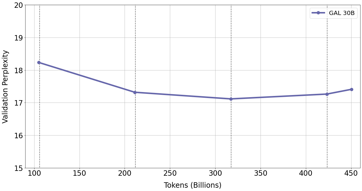
We observe falling validation perplexity up until the start of the fourth epoch, at which point the model overfits for this particular dataset. This may suggest Galactica is getting worse at more "out-of-domain" proteins that differ significantly from the test set. For future work, less repetition is probably desirable; and more generally, increasing the diversity of proteins in the training dataset is likely to be beneficial.

5.7.2 Functional Keyword Prediction

We now look at specific translation capabilities from protein sequence toward natural language, which may be useful for tasks such as protein annotation. As a first test, we look at UniProt keywords that Galactica can infer from the sequence. An example of these is shown in Figure 20 overleaf.

Figure 19: Protein Keyword Prediction. This test’s Galactica’s capability to predict protein keywords, e.g. "cytoplasm", from the sequence alone. For the Paen and General datasets, this capability improves smoothly with scale. It scales more slowly and begins to saturate for the CASPSimSeq set, reflecting the lower sequence similarity with sequences in the training set.

Figure 20: Protein Keyword Prediction. Example shown is Q108U0 from the PaenSeq holdout, a cystic fibrosis transmembrane conductance regulator from the African elephant. The closest protein by sequence similarity in the training set is the Q2QLA3 protein, a cystic fibrosis transmembrane conductance regular from a horse, with 91.8% sequence similarity.

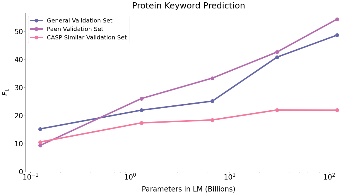
We report results in Table 17. $F_1$ score increases across the holdout sets with scale, suggesting that Galactica can learn keywords by inferring from the sequence. However, we see saturation for the CASPSimSeq, suggesting this capability depends on how similar the sequences are to those in the training set. This is reflected in the example in Figure 20, where Galactica uses its knowledge of a similar proteins from different organisms, with a maximum sequence similarity of 91.8% in the training set, to help annotate.

Protein Keyword Prediction
Model	Param (bn)	CASPSimSeq	PaenSeq	UniProtSeq
GAL 125M	0.1	10.5%	9.3%	15.2%
GAL 1.3B	1.3	17.4%	26.0%	21.9%
GAL 6.7B	6.7	18.4%	33.3%	25.1%
GAL 30B	30	22.0%	42.6%	40.8%
GAL 120B	120	21.9%	54.5%	48.7%

Table 17: Protein Keyword Prediction. Metric shown is $F_1$ score. Performance increases with scale across the holdout sets. Note we do not include CASPSeq as these do not have UniProt keywords we can test against.

We attempted to visualize attention in the protein sequence, but we did not observe anything with biological intepretation (e.g. attention to domains). Our working hypothesis is that Galactica has learnt an implicit measure of sequence similarity that it uses to associate predicted keywords, but that this is not directly interpretable from where it attends to. This differs from our chemistry analysis where results were interpretable in terms of attention to the underlying atomic structure.

5.7.3 Protein Function Description

As the next test, we look at generating free-form descriptions of protein function from the sequence. We look at the UniProt function descriptions and compare to Galactica generated descriptions.

We report results in Table 18. ROUGE-L score increases smoothly across all the holdout sets. We show an example overleaf in Figure 21 from PaenSeq. The protein is a Cytochrome b protein from a rock hyrax (Q7Y8J5). The closest sequence by similarity in the training set is a Cytochrome b protein from a pygmy hippopotamus (O03363) with 83% sequence similarity. In this case we get a perfect prediction from the description.

Protein Function Prediction
Model	Param (bn)	CASPSimSeq	PaenSeq	UniProtSeq
GAL 125M	0.1	0.062	0.073	0.061
GAL 1.3B	1.3	0.069	0.084	0.079
GAL 6.7B	6.7	0.109	0.137	0.111
GAL 30B	30	0.137	0.196	0.186
GAL 120B	120	0.252	0.272	0.252

Table 18: Protein Function Prediction. Metric shown is ROUGE-L. Performance increases with scale.

Figure 21: Protein Description Prediction. Example shown is Q7Y8J5 from the PaenSeq holdout, a Cytochrome b protein from a rock hyrax. The closest protein by sequence similarity in the training set is the O03363 protein, a Cytochrome b protein from a pygmy hippopotamus, with 83% sequence similarity.

As with the keyword prediction task, Galactica appears to be learning based on matching sequences with similar ones it has seen in training, and using this to form a description. This suggests language models for protein sequences could serve as useful alternatives to existing search methods such as BLAST and MMseqs2 (Altschul et al., 1990; Steinegger and Söding, 2017).

6 Toxicity and Bias

In this section we study the toxicity and bias of the Galactica model. We evaluate on benchmarks related to stereotypes, toxicity, and misinformation. We compare results to other language models. We find Galactica is significantly less biased and toxic than existing language models.

6.1 Bias and Stereotypes

For the following evaluations, we investigate Galactica’s ability to detect (and generate) harmful stereotypes and hate speech, using four widely used benchmarks.

6.1.1 CrowS-Pairs

CrowS-Pairs
Bias type	text-davinci-002	OPT 175B	Galactica 120B
Race	64.7	68.6	59.9
Socioeconomic	73.8	76.2	65.7
Gender	62.6	65.7	51.9
Disability	76.7	76.7	66.7
Nationality	61.6	62.9	51.6
Sexual-orientation	76.2	78.6	77.4
Physical-appearance	74.6	76.2	58.7
Religion	73.3	68.6	67.6
Age	64.4	67.8	69.0
Overall	67.2	69.5	60.5

Table 19: CrowS-Pairs Results. Galactica demonstrates significantly lower stereotypical bias in all categories with the exception of sexual orientation and age.

CrowS-Pairs is a collection of 1,508 crowd-sourced pairs of sentences, one which is "more" stereotyping and one which is "less" stereotyping, and covers nine characteristics (Nangia et al., 2020). These characteristics are race, religion, socioeconomic status, age, disability, nationality, sexual orientation, physical appearance, and gender. A language model’s preference for stereotypical content is measured by computing the proportion of examples in which the "more" stereotypical sentence is preferred (as determined by log likelihood). Higher scores indicate a more harmfully biased model, whereas an ideal model with no bias would score 50%.

We report results for Galactica and other language models in Table 19. Galactica exhibits significantly lower stereotypical biases in most categories, with the exception of sexual orientation and age, when compared to the latest GPT-3 (text-davinci-002) and OPT 175B. Galactica attains a better overall score of 60.5% compared to the other models. Language models such as OPT use the Pushshift.io Reddit corpus as a primary data source, which likely leads the model to learn more discriminatory associations (Zhang et al., 2022). Galactica is trained on a scientific corpus where the incidence rate for stereotypes and discriminatory text is likely to be lower.

6.1.2 StereoSet

StereoSet
Category		text-davinci-002	OPT 175B	Galactica 120B
	LMS ($\uparrow$)	78.4	74.1	75.2
Prof.	SS ($\downarrow$)	63.4	62.6	57.2
	ICAT ($\uparrow$)	57.5	55.4	64.3
	LMS ($\uparrow$)	75.6	74.0	74.6
Gend.	SS ($\downarrow$)	66.5	63.6	59.1
	ICAT ($\uparrow$)	50.6	53.8	61.0
	LMS ($\uparrow$)	80.8	84.0	81.4
Reli.	SS ($\downarrow$)	59.0	59.0	55.1
	ICAT ($\uparrow$)	66.3	68.9	73.1
	LMS ($\uparrow$)	77.0	74.9	74.5
Race	SS ($\downarrow$)	57.4	56.8	54.8
	ICAT ($\uparrow$)	65.7	64.8	67.3
	LMS ($\uparrow$)	77.6	74.8	75.0
Overall	SS ($\downarrow$)	60.8	59.9	56.2
	ICAT ($\uparrow$)	60.8	60.0	65.6

Table 20: StereoSet Results. Galactica outperforms all models across all categories on the ICAT score.

StereoSet aims to measure stereotypical biases across profession, religion, gender, and race (Nadeem et al., 2021). The benchmark contains two tasks: an intrasentence task and an intersentence task, with around 2,100 examples each in the development set.

• Intrasentence Task: the stereotype and associated context are in the same sentence.

• Intersentence Task: the context and stereotype are in different (consecutive) sentences.

Alongside stereo- and anti-stereotypical variants of sentences, each example in StereoSet contains an unrelated sentence. This sentence is included for measuring a Language Modelling Score (LMS) and a Stereotype Score (SS). These two metrics are combined to form the Idealized Context Association Test score (ICAT), which is a balanced measure of bias detection and language modeling. An ideal, unbiased language model would score an LMS of 100, an SS of 50, and an ICAT of 100.

We report results in Table 20. Galactica outperforms other models on all categories for the overall ICAT score.

6.1.3 Toxicity

Figure 22: Toxicity rate on RealToxicityPrompts. Galactica exhibits much lower toxicity continuation rates, even as we increase the original prompt toxicity.

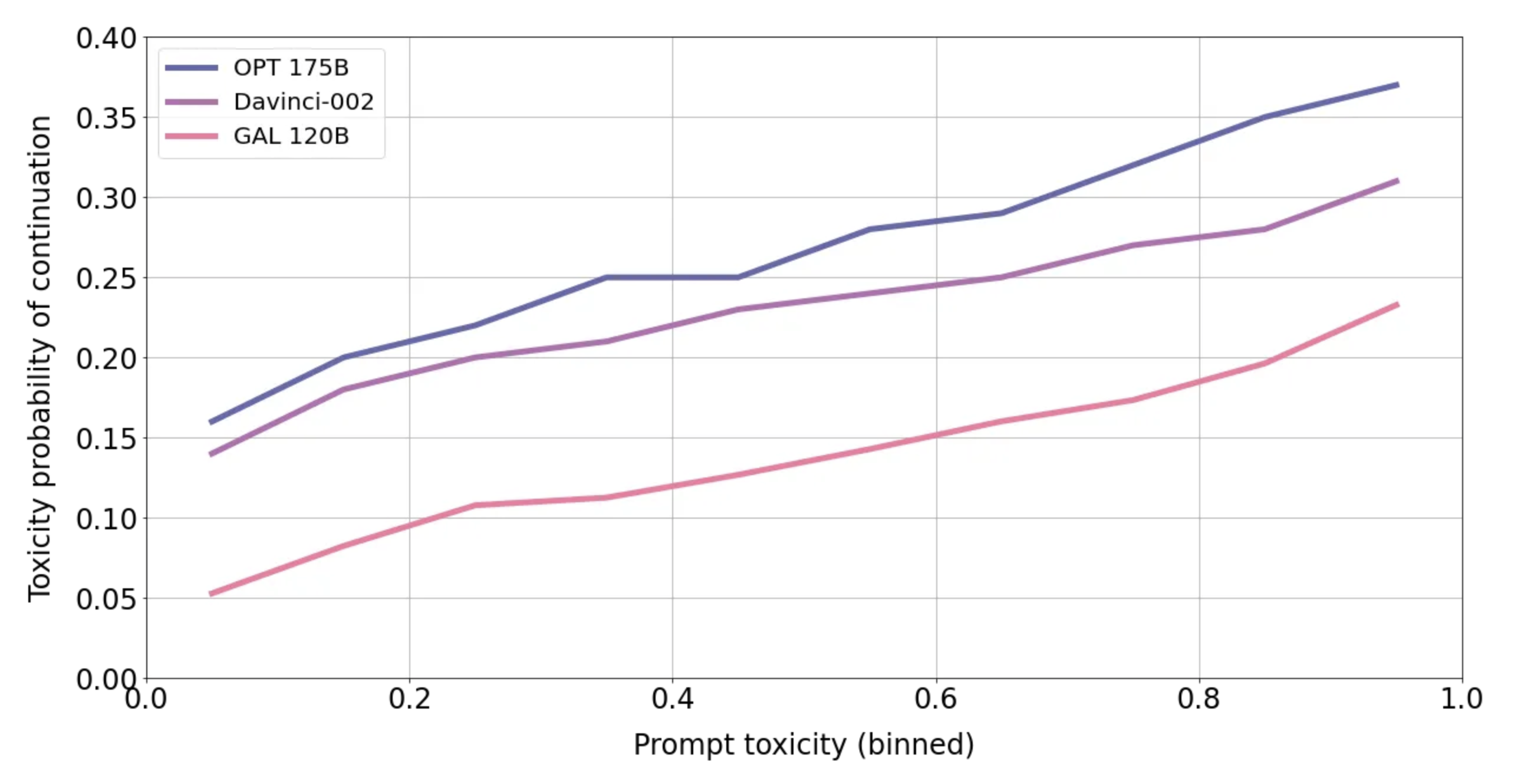
To measure toxicity we use the RealToxicityPrompts (RTP) benchmark introduced in Gehman et al. (2020). We follow the same setup of Zhang et al. (2022) and sample 25 generations of 20 tokens using nucleus sampling (p=0.9) for each of 5000 randomly sampled prompts from RTP. We use the prompts to produce sequences (i.e, continuations) which are then scored by a toxicity classifier provided by Perspective API.

Figure 22 plots the results. The chart shows the mean toxicity probability of continuations (y-axis), stratified across bucketed toxicities of the original prompts (x-axis). Galactica exhibits substantially lower toxicity rates than the other models.

6.2 TruthfulQA

TruthfulQA is a benchmark that measures answer truthfulness of language model generations (Lin et al., 2022a). It comprises 817 questions that span health, law, finance and other categories. We compare to other published language models. We report results in Table 21. Galactica exceeds the performance of other language models on this benchmark. However, absolute performance is still low. Given the curated nature of our corpus, this suggests that data alone does not cause language models to struggle at this task.

TruthfulQA
Model	MC1 (Acc)	MC1 (Std)
OPT 175B	21%	0.13
BLOOM 176B	19%	0.07
GAL 125M	19%	0.11
GAL 1.3B	19%	0.15
GAL 6.7B	19%	0.03
GAL 30B	24%	0.05
GAL 120B	26%	0.02

Table 21: TruthfulQA Results. Galactica exhibits superior performance to other language models, and performance increases with scale. but slowly and at low levels.

7 Limitations and Future Work

7.1 Limitations

We cover some of the limitations with work in this section.

Corpus Limitations

Our corpus has several limitations, both external and internally imposed. The main external constraint is our restriction to use open-access resources, and much of scientific knowledge like papers and textbooks are not open access. With access to these closed sources of knowledge, performance is likely to be considerably higher. We also use self-imposed constraints, like restricting the number of molecules and proteins for this work; without these constraints, we are likely to see considerable performance gains due to much larger corpuses for these modalities.

Corpus Effects vs Prompt Effects

In several benchmarks, we show performance gains over existing language models, but we do not specifically disentangle the effects of the prompts we included in pre-training versus the core scientific corpus. In future work, we likely need to disentangle these effects in order to see whether general language capabilities are possible with a scientific corpus alone without prompt boosting.

Citation Bias

While we demonstrate that the model approaches the true citation distribution with scale, some bias towards popular papers still remains with the 120B scale model, so the model likely requires augmentation before being used in a production environment.

Prompt Pre-Training vs Instruction Tuning

We opted for the former in this paper, but ideally we would need to explore what the latter could achieve, along the lines of the recent work of Chung et al. (2022). A limitation of this work is that we do not perform this direct comparison through ablations, making clear the trade-offs between approaches.

General Knowledge

While Galactica absorbs broad societal knowledge through sources such as Wikipedia - e.g. 120B knows Kota Kinabalu is the capital of Malaysia’s Sabah state - we would not advise using it for tasks that require this type of knowledge as this is not the intended use-case.

Text as a Modality

While we have shown text-based Transformers are surprisingly powerful with text representations of scientific phenomena, we caution against the interpretation that text is all you need. For example, in chemistry, geometry is a fundamental language that determines meaning, yet Galactica has no notion of geometry; e.g. 3D co-ordinates of atoms.

7.2 Future Work

For development of the base model, we highlight several directions that may be worth pursuing.

New Objective Function

It is likely further gains can be obtained with mixture-of-denoising training as U-PaLM has recently shown (Tay et al., 2022b; Chung et al., 2022). We suspect this might be beneficial for the scientific modalities such as protein sequences, where the left-to-right LM objective is quite limiting.

Larger Context Window

We use a maximum context window length of $2048$ tokens in this work. Extending this is likely to be beneficial for understanding in long-form scientific documents, such as textbooks and also documents with longer modality sequences (e.g. long protein sequences).

Extending to Images

We cannot capture scientific knowledge adequately without capturing images. This is a natural follow-up project, although it likely requires some architectural modification to make it work well. Existing work such as Alayrac et al. (2022) has shown how to extend LLMs with this modality.

More <work> examples

We feel <work> could be a general-purpose reasoning token and we would like to invest more in this direction, including increasing prompt diversity and exploring performance on more benchmarks.

Verification

Even as language models become more accurate with scale, we need assurances that their generations are correct and factual. Developing this layer is critical for production applications of language models in general beyond scientific applications.

Continual Learning

Should we re-train from scratch to incorporate new scientific knowledge or train from older checkpoints? This is an open question, and further research is needed to find the best procedure for incorporating new knowledge into the model.

Retrieval Augmentation

While we have shown how large language models can absorb large bodies of scientific knowledge, retrieval has a place for fine-grained types of knowledge, and we believe this is a strong direction to pursue to complement the flexible weight memory of the Transformer.

8 Discussion and Conclusion

For over half a century, the dominant way of accessing scientific knowledge has been through a store-and-retrieve paradigm. The limitation of this approach is the reasoning, combining and organization of information still relies on human effort. This has led to a significant knowledge throughput bottleneck. In this work we explored how language models might disrupt this paradigm and bring about a new interface for humanity to interface with knowledge.

We showed that language models are surprisingly strong absorbers of technical knowledge, such as LaTeX equations and chemical reactions, and these capabilities tend to scale smoothly with model size. The context-associative power of language models likely confers significant advantages over search engines in the long-run. We demonstrated this for citation prediction, where a language model outperforms tuned sparse and dense retrieval pipelines for this task. Language models will likely provide a valuable new tool for exploring the literature and the body of scientific knowledge in coming years.

We also demonstrated that language models can compose a curated knowledge base to perform well in knowledge-intensive question answering tasks. This includes composing knowledge in a step-by-step reasoning manner. We showed that with a working memory token approach, we can achieve strong performance over existing methods on mathematical MMLU and MATH benchmarks. We suspect tasks like MATH are in principle solvable with language model approaches. The current bottleneck is the availability of high quality step-by-step datasets. However, language models will not perform these tasks like humans until they have an architectural change that supports adaptive computation.

We also performed initial investigations on the potential of LLMs to act as a bridge between scientific modalities and natural language. We showed Galactica could learn tasks like IUPAC naming through self-supervision. We also showed that it is possible to formulate drug discovery tasks like MoleculeNet in a natural language prompt and achieve strong results without direct fine-tuning. Lastly, we showed the potential for tasks such as automatic protein annotation. In all, increasing the number (and size) of datasets that bridge between natural language and natural sequences is likely to boost performance further.

Taken together, we feel there is a strong potential for language models to take on knowledge tasks that are currently human specialisms. We open source the models so others can build on our work, and we look forward to seeing how the open machine learning community will extend it.

Appendix A Appendix

A.1 Dataset Components

We cover the various components of the corpus in this section.

A.1.1 Papers

We source scientific papers from preprint servers such as arXiv, PMC and other sources; see Table 22.

We also use the Semantic Scholar full text dataset (S2) to capture the long tail of science (Lo et al., 2019a). We apply several quality filters, including excluding papers from journals with certain keywords, and also excluding papers with a low journal impact factor. Details of the filters we used are contained in the Appendix.

We source abstracts where full texts are not open access. In total the full dataset contains 48 million papers, abstract and full-text, up to July 2022.

Data source	Documents	Tokens
arXiv	2 million	35 billion
PMC	3 million	23 billion
Semantic Scholar	3 million	18 billion
PubMed Abstracts	21 million	5 billion
Semantic Scholar Abstracts	19 million	4 billion
bioRxiv	128,059	1 billion
OSF	54,905	428 million
medRxiv	24,019	176 million
ACL	25,518	150 million
PubAg Abstracts	308,235	105 million
ChemRxiv	7,617	67 million
Total	48 million	88 billion

Table 22: Paper sources used in our corpus

We use a modified version of the GROBID library for converting PDFs to text, as well as obtaining titles, authors and citations (GROBID, 2008–2022). Where mathematical LaTeX is available, for example in arXiv, we make sure to combine the GROBID results with LaTeX source to recover mathematical content.

The final paper documents are stored in a markdown format, as opposed to full LaTeX. We use markdown as the standard format for all documents in the corpus to support knowledge blending between sources. Papers are citation processed, following the title-based approach of Section 2.2.

A.1.2 Reference Material

We source encyclopedias, textbooks and educational material to create a base of reference material that the model can learn from. The details are covered in Table 23.

Data source	Documents	Tokens
Wikipedia	6 million	5 billion
StackExchange	1.6 million	1 billion
LibreText	95,113	185 million
Wikibooks	74,705	110 million
Open Textbooks	647	94 million
MIT OCW	25,640	90 million
Wikiversity	38,138	52 million
ProofWiki	32,389	12 million
Khan Academy	3,075	7 million
Papers with Code	13,430	4 million
IUPAC Goldbook	6,788	1 million
Total	8 million	7 billion

Table 23: Reference material used in our corpus

We apply source specific processing for several of the datasets, specifically:

• For StackExchange, we take questions from scientific sites; see the Appendix for the subset used.

• For Papers with Code and IUPAC Goldbook we apply data augmentation in the form of prompt randomization. Sometimes we pose sections as questions/answers; for example a section explaining a machine learning method is sometimes posed as "Question: What is [method]?".

• For KhanAcademy articles, we add <work> tokens for step-by-step reasoning examples, which we explain shortly in Section 2.4.

We make an effort to preserve mathematical LaTeX and capture citations, including hyperlinks to papers.

A.1.3 Knowledge Bases

We source fine-grained knowledge from scientific knowledge bases. The details are covered in Table 24.

Data source	Documents	Tokens
PubChem Compound	1.7 million	1 billion
UniProt	551,837	0.6 billion
RefSeq Genome	69	0.1 billion
OEIS	350,833	0.07 billion
Ribosome	9,950	0.05 billion
LIPID MAPS	45,273	0.03 billion
Reactome	156	0.01 billion
NASA Exoplanet	5,021	0.01 billion
Total	2 million	2 billion

Table 24: Knowledge bases used in our corpus

For the chemistry and biology datasets, we wrap modalities like SMILES and protein sequences with their specialized tokens (see Section 2.1). For UniProt we apply data augmentation to the document format:

• Order Randomization - with probability $0.5$ the protein sequence starts at beginning of the document, else the end of document. This ensures we can learn from $\text{seq}\to \text{property}$ and $\text{property}\to \text{seq}$.

• Format Randomization - with probability $\frac{1}{3}$ we replace a description, e.g. "The function of protein is…", with a Q&A, e.g. "Question: What is the function of the protein? Answer: The function is…".

For NASA Exoplanet we apply order randomization to the exoplanet characteristics.

For chemical and biological sequences, we take a small subset of available entities. This is to ensure the model is not overly biased towards learning natural sequences over natural language. Specifically:

• For PubChem Compound, we take a small, random subset ($2$ million) of total compounds ($110$ million).

• For UniProt, we take reviewed Swiss-Prot proteins; a small subset ($0.5$ million) of total ($227$ million).

• For RefSeq Genome, we take reference sequences, which is a small subset of available nucleotide sequences. For the human genome, we only include the protein-coding genes.

This is a constraint we can relax in future work, enabling for much larger corpus. In this work, we focus on the first step of investigating whether a single model can learn effectively in this multi-modal setting.

A.1.4 Common Crawl

We source academic and scientific content via a highly-filtered subset of CommonCrawl. The details are covered in Table 25.

Data source	Documents	Tokens
ScientificCC	0.8 million	0.7 billion
AcademicCC	0.05 million	0.4 billion
Total	0.9 million	1.1 billion

Table 25: CommonCrawl material used in our corpus

For Scientific Common Crawl, we train a fasttext classifier to identify Common Crawl webpages with scientific content (Joulin et al., 2016) using a noisy set of 600 domains. We then manually annotated the domains predicted by fasttext as scientific to assemble a list of 200 high-quality scientific and reference domains.

For Academic Common Crawl, we assemble a list of academic domains, such as university websites. We take PDFs from these domains, based on the Common Crawl index, and process these using GROBID.

We do not LaTeX-process pages from these sources.

We found the quality of extracted text in CommonCrawl generally quite poor, which is why we applied stringent filters. We suspect this could be an important area for future work in order to capture more base scientific knowledge.

A.1.5 Code

We source academic GitHub repositories from the Papers with Code index for machine learning, physics, mathematics, statistics and astronomy. The index does not explicitly cover sciences such as biology and chemistry, but many of these repositories are captured as part of the general machine learning index. We exclude repositories that do not have a license or copyright file.

A.1.6 <work> Datasets

For KhanProblems, we used the problems from AMPS and converted to a <work> format (Hendrycks et al., 2021). Where possible we tried to include more tedious steps to reduce errors from a single pass, but this annotation was fairly incomplete and we suspect bigger gains are possible with more cleaning.

For GSM8k we use the provided training dataset and convert so the calculator steps are performed by writing a Python program, following the <work> format (Cobbe et al., 2021). In general, we found when the model went into this prompt style, it was more error-prone. We think this is because the prompt style made the model write too many programs within <work>, rather than getting things ready to run in a single program. In general we found longer <work> answers led to a higher chance of a mistake on the reasoning path.

For OneSmallStep, we made 50 problem set question templates, and randomized the variables in the problem to get more prompt examples. We summarize the fields we made prompts below.

Field	Templates
Astronomy	2
Chemistry	7
Electronics	10
Mathematics	15
Physics	14
Statistics	2
Total	50

As we can see the diversity was not very large, and so further gains are likely with more annotation.

Lastly we wrote 921 examples, based off internet examples, in a <work> format for Workout. This was our highest quality dataset, and had reasonable diversity across fields: mathematics, chemistry, biology, astronomy, physics, geology, history. This is the type of dataset we would look to scale in future work.

A.2 Dataset Deduplication

We use the following procedure for deduplicating the corpus:

• We identify identical spans of 100 bytes or more (of utf-8 text) across the whole corpus, except for some explicitly excluded data sources. We do this using the repository from Lee et al. (2022).

• We process corpus files in a predetermined order to prioritize some sources. From a set of spans representing the exact same content across files, we remove the span in the first file. If the same content repeats across a single file and it was not found in the files before, all its occurrences are kept.

• We merge duplicated spans separated by at most 4 bytes.

• We narrow down the resulting spans to paragraph boundaries (i.e. "\n\n").

• We remove the content from files corresponding to the spans.

A.3 Citation Identifier Ablations

We report ablations for the citation identifier ablations below, where we test title-based identifiers versus alphanumeric identifiers.

Specifically, we set up an evaluation set of dataset and method names from Papers with Code. The task is to predict the citation given the method or dataset name, e.g. ResNet [START_REF], where the target is Deep Residual Learning for Image Recognition, He. We train a 6.7bn model on both types of processing for the ablation. Method and dataset results are shown below.

	Citation Processing
	(a) Titles			(b) IDs
Method citations	Correct	Hallucinated	Incorrect	Correct	Hallucinated	Incorrect
$k=1$	13.8%	54.5%	31.7%	1.8%	3.5%	94.7%
2	30.4%	38.6%	31.1%	9.3%	4.0%	86.7%
5	36.3%	29.5%	34.2%	17.9%	0.0%	82.1%
10	43.0%	15.8%	41.2%	38.8%	3.0%	58.2%
25	53.4%	8.7%	37.9%	43.7%	0.0%	56.3%
50	64.8%	9.9%	25.3%	60.6%	1.4%	38.0%
100	64.6%	8.3%	27.1%	63.5%	1.0%	35.4%
$\ge 500$	78.6%	0.0%	21.4%	78.6%	0.0%	21.4%

Table 26: Citation Processing Ablation. We predict citations for the PWC Methods dataset using 6.7 billion size models. Papers are bucketed according to the number of citations (mentions) in the dataset. The title processing model has a higher accuracy, but greater risk of hallucination. There are 1,705 methods in this evaluation dataset.

	Citation Processing
	(a) Titles			(b) IDs
Dataset citations	Correct	Hallucinated	Incorrect	Correct	Hallucinated	Incorrect
$k=1$	1.4%	62.5%	36.1%	0.5%	11.5%	88.1%
	5.0%	59.2%	35.8%	0.6%	10.2%	89.2%
	15.4%	49.7%	34.8%	2.6%	6.2%	91.1%
	25.7%	36.8%	37.5%	8.3%	4.8%	86.9%
	44.6%	27.4%	28.0%	22.9%	7.0%	70.0%
	58.6%	17.7%	23.6%	41.4%	7.7%	50.9%
	65.5%	6.7%	27.8%	62.4%	3.1%	34.5%
$\ge 500$	81.8%	6.1%	12.1%	81.8%	3.0%	15.2%

Table 27: Citation Processing Ablation. We predict citations for the PWC Datasets dataset using 6.7 billion capacity models. There are 4,735 datasets in this evaluation dataset.

A.4 120B Validation Loss Per Source

Figure 23: Validation Loss Per Source. Validation loss falls through training for all dataset categories. Results are shown for the 120B model above.

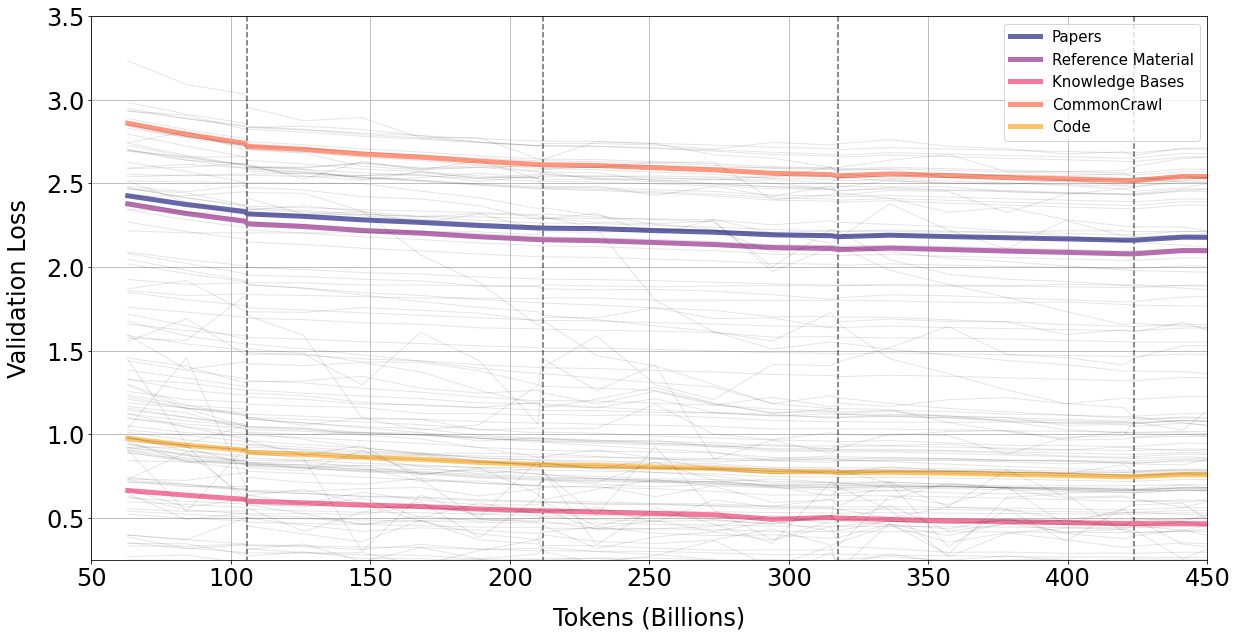
A.5 Chain-of-Thought vs <work>

We used the recent results by Chung et al. (2022) of PaLM 540B on the MMLU validation set (Hendrycks et al., 2020) for comparison. While use of reasoning degrades performance versus direct prompting for both approaches, the <work> token appears more robust.

Chain-of-Thought versus <work>
Subject	Examples	PaLM 540B CoT	GAL 30B <work>	GAL 120B <work>
Abstract Algebra	11	9.1%	27.3%	27.3%
Astronomy	16	7.1%	43.8%	25.0%
College Chemistry	8	12.5%	37.5%	37.5%
College Computer Science	11	9.1%	45.5%	54.6%
College Mathematics	11	0.0%	36.4%	18.2%
College Physics	11	36.4%	36.4%	45.5%
Econometrics	11	33.3%	33.3%	33.3%
Electrical Engineering	16	18.8%	37.5%	56.3%
Elementary Mathematics	41	24.4%	53.7%	58.5%
Formal Logic	9	0.0%	21.4%	21.4%
High School Chemistry	22	22.7%	27.3%	36.4%
High School Computer Science	9	33.3%	44.4%	44.4%
High School Mathematics	29	24.1%	31.0%	51.7%
High School Physics	17	11.8%	23.5%	29.4%
High School Statistics	23	26.1%	39.1%	56.5%
Machine Learning	11	18.2%	9.1%	27.3%
Overall	261	19.1%	35.9%	42.4%

Table 28: <work> vs Chain-of-Thought. PaLM is evaluated with CoT 5-shot. Galactica with the <work> token included in pre-training. Results here are on MMLU dev for comparability with PaLM.

BIG-bench
Benchmark	OPT 30B	OPT 175B	BLOOM 176B	GAL 30B	GAL 120B
Anachronisms	47.4%	49.1%	1.3%	47.0%	48.7%
Analogical Similarity	12.7%	19.8%	19.2%	17.0%	23.5%
Analytic Entailment	40.0%	52.9%	48.6%	47.1%	51.3%
Causal Judgment	53.7%	55.3%	54.7%	49.5%	51.1%
Crash Blossom	42.1%	36.8%	47.4%	42.1%	42.1%
Crass AI	20.5%	34.1%	31.8%	40.9%	52.3%
Dark Humor Detection	46.3%	48.8%	51.3%	48.8%	46.3%
Date Understanding	15.5%	21.1%	12.2%	11.4%	16.8%
Disambiguation QA	39.5%	44.6%	44.2%	46.9%	43.0%
Empirical Judgments	38.4%	52.5%	56.6%	50.5%	54.6%
English Proverbs	26.5%	20.6%	26.5%	26.5%	17.7%
Entailed Polarity	87.8%	88.5%	89.2%	89.2%	85.8%
Epistemic Reasoning	43.4%	43.5%	61.2%	40.1%	53.0%
Evaluating Information Essentiality	32.4%	19.1%	29.4%	25.0%	22.1%
Fantasy Reasoning	67.7%	69.2%	65.2%	66.7%	52.7%
Figure of Speech Detection	10.2%	13.6%	22.0%	13.6%	15.3%
General Knowledge	51.4%	78.6%	80.0%	68.6%	74.3%
GRE Reading Comprehension	6.5%	12.9%	22.6%	16.1%	35.5%
Hindu Knowledge	32.6%	42.3%	48.6%	36.6%	49.7%
Human Organs Senses	45.2%	57.1%	59.5%	71.4%	73.8%
Identify Odd Metaphor	27.7%	21.3%	19.2%	19.2%	27.7%
Implicatures	44.3%	49.6%	53.7%	59.4%	69.9%
Implicit Relations	22.4%	35.3%	28.2%	16.5%	25.9%
Intent Recognition	66.2%	79.2%	89.5%	87.8%	89.5%
Irony Identification	50.5%	49.5%	63.6%	60.6%	59.6%
Known Unknowns	50.0%	52.2%	50.0%	50.0%	41.3%
Logic Grid Puzzle	32.7%	31.6%	31.1%	35.8%	39.4%
Logical Args	18.8%	34.4%	25.0%	34.4%	43.8%
Logical Fallacy Detection	50.9%	54.9%	54.5%	54.1%	55.1%
Logical Sequence	38.5%	46.2%	30.8%	25.6%	43.6%
Mathematical Induction	60.9%	55.1%	52.2%	44.9%	58.0%
Metaphor Boolean	51.1%	57.5%	61.5%	63.4%	49.1%
Misconceptions	56.1%	57.5%	54.8%	51.6%	58.0%
Moral Permissibility	50.6%	54.4%	57.0%	52.3%	49.7%
Movie Recommendation	6.4%	52.6%	49.4%	31.6%	36.8%
Navigate	49.3%	49.8%	51.1%	50.9%	51.8%
Nonsense Words Grammar	28.0%	46.0%	48.0%	38.0%	48.0%
Novel Concepts	9.4%	12.5%	15.6%	6.3%	9.4%
Odd One Out	30.2%	26.7%	22.1%	12.8%	19.8%
Penguins in a Table	29.5%	32.9%	28.2%	40.9%	36.9%
Phrase Relatedness	45.0%	51.0%	55.0%	53.0%	64.0%
Physical Intuition	39.5%	42.0%	37.0%	55.6%	58.0%
Physics	39.3%	42.8%	54.2%	55.9%	65.5%
Presuppositions as NLI	36.6%	36.2%	39.6%	34.0%	28.0%
Question Selection	39.8%	42.1%	5.2%	41.1%	42.7%
Reasoning about Colored Objects	33.9%	38.7%	40.5%	45.8%	55.0%
Riddle Sense	40.8%	57.1%	44.9%	46.9%	42.9%
Ruin Names	19.4%	20.8%	12.5%	24.1%	33.0%
Sentence Ambiguity	63.3%	60.0%	65.0%	60.0%	66.7%
Similarities Abstraction	21.1%	22.4%	27.6%	21.1%	13.2%
Snarks	42.0%	41.4%	47.0%	48.1%	48.6%
Sports Understanding	50.0%	48.8%	54.5%	52.0%	51.8%
StrategyQA	56.1%	58.5%	57.1%	53.9%	53.7%
Temporal Sequences	31.4%	28.4%	20.5%	26.4%	21.2%
Timedial	15.3%	22.2%	24.4%	39.9%	40.8%
Understanding Fables	20.1%	19.6%	24.9%	28.0%	20.1%
Winowhy	37.2%	39.7%	38.0%	56.5%	56.4%
Average (weighted)	39.6%	43.4%	42.6%	46.6%	48.7%
Average (unweighted)	32.8%	42.7%	42.2%	42.7%	45.3%

Table 29: BIG-bench Results. Galactica exceeds the performance of general models, even at lower scales.

A.6 Prompt Pre-training Datasets

We report the prompt datasets we included in pre-training below.

Data source	Split	Prompts	Tokens
MedMCQA (Pal et al., 2022)	train	180,894	13,311,290
RACE (Xu et al., 2017)	train	29,502	12,160,390
Quoref (Dasigi et al., 2019)	train	19,206	10,361,335
ROPES (Lin et al., 2019)	train	10,815	2,672,195
BioASQ7 task b (Nentidis et al., 2021)	train	2,676	1,288,462
TQA (Kembhavi et al., 2017)	train	8,566	1,856,473
BoolQ (Clark et al., 2019)	train	9,333	1,224,335
SciQ (Welbl et al., 2017)	train	10,346	1,397,668
QASC (Khot et al., 2020)	train	8,053	930,414
CommonSenseQA (Talmor et al., 2018)	train	9,644	660,750
OpenBookQA (Mihaylov et al., 2018)	train	4,908	324,995
QCScience (V et al., 2021)	train	2,417	209,803
PubMedQA (Jin et al., 2019)	train	495	186,304
QASPER (Dasigi et al., 2021)	train	606	105,985
UChallenge (new)	train	346	29,308
TrueOrFalse (new)	train	107	2,854

Table 30: Question answering prompts used in Naturebook

Data source	Split	Prompts	Tokens
JNLPBA (Kim et al., 2004)	train	91,213	5,262,723
BC4CHEMD (Krallinger et al., 2004)	train	30,234	1,756,929
ChemProt (Taboureau et al., 2011)	train	3,030	1,286,816
BC2GM (Smith et al., 2008)	train	12,375	704,357
S800 (Pafilis et al., 2013)	train	5,318	281,448
BC5CDR Chem (Li et al., 2016)	train	4,503	241,729
BC5CDR Disease (Li et al., 2016)	train	4,498	231,322
MethodNet (new)	train	659	167,904
Scientific Entities (new)	train	305	97,935

Table 31: Entity extraction prompts used in Naturebook

Data source	Split	Prompts	Tokens
PWC Desc (new)	train	3,586	9,663,419
SciTail (Khot et al., 2018)	train	23,361	1,383,614
Fragmented Glass (new)	train	718	867,985
SciTLDR (Cachola et al., 2020)	train	1,973	472,169

Table 32: Summarization prompts used in Naturebook

Data source	Split	Prompts	Tokens
Wizard of Wikipedia (Dinan et al., 2018)	train	18,246	4,466,113
Advising (Gunasekara et al., 2019)	train	495	147,793

Table 33: Dialog prompts used in Naturebook

Data source	Split	Prompts	Tokens
BACE Classification	train	1,198	122,699
BACE Regression	train	1,198	154,656
BBBP	train	1,613	115,916
ClinTox	train	1,171	100,955
Delaney	train	893	62,083
FreeSolv	train	508	29,542
HIV	train	32,572	2,308,966
HOPV	train	2,217	333,620
Lipo	train	3,327	362,342
PCBA	train	714,277	553,645,656
QM7	train	5,416	320,199
QM8	train	275,569	27,163,516
QM9	train	1,259,090	128,427,073
SAMPL	train	508	1,259,090
SIDER	train	30,499	2,741,904
Thermosol	train	1,396	139,481
Tox21	train	73,883	54,224,093

Table 34: Chemical property prediction prompts used in Naturebook

A.6.1 Chemical Property Prediction

We set up a prediction task for chemical and physical properties with our validation set of 17,052 compounds. We use the PubChem document structure to design a prompt. We show an example for XLogP in Figure 24.

Figure 24: Chemical Property Prompt. We design a prompt based on the PubChem document format. Using this prompt style, we test the model’s ability to learn chemical and physical properties from the SMILES sequence.

We report results in Table 35. The error decreases fairly smoothly with scale, suggesting self-supervised learning is occurring within-document from SMILES towards the chemical and physical properties. But it tails off for 120B which suggests more molecule data might be needed.

Chemical and Physical Property Prediction
Model	Param (bn)	Mol. Weight	XLogP	Rotatable Bond #	Topological PSA
GAL 125M	0.1	101.43	1.638	4.389	36.63
GAL 1.3B	1.3	101.05	1.413	3.930	41.11
GAL 6.7B	6.7	81.76	1.197	2.932	30.01
GAL 30B	30	77.46	1.101	3.534	29.54
GAL 120B	120	86.57	1.131	3.474	28.84

Table 35: Chemical and physical property prediction. All results reported as RMSE. Prediction error generally decreases with scale, indicating Galactica can infer properties from SMILES.

A.6.2 Docking Regression

We looked briefly at the docking score regression task (García-Ortegón et al., 2022). Here the task is to predict a docking score based on an target and a ligand. In the case of Galactica, we use a text format to represent this information. An example is shown in Figure 25. We report results in Table 36.

Figure 25: DockSTRING Format. To construct the training set, we take the protein target and ligand sequences, pose a natural language question, and have the docking score as the answer.

Docking Regression
Model	Param (bn)	ESR2	F2	KIT	PARP1	PGR
GAL 125M	0.1	-12.4	-6.09	-6.73	-1.69	-12.4
GAL 1.3B	1.3	-0.293	0.591	0.063	0.728	-1.72
GAL 6.7B	6.7	-0.216	0.694	0.290	0.681	-0.894
GAL 30B	30	-0.186	0.679	0.313	0.732	-0.468
GAL 120B	120	-0.564	0.626	0.249	0.732	-0.960

Table 36: DockSTRING Results. Metric shown is $R^2$.

For three of the targets, Galactica is able to infer from looking at the sequences alone, and performance scales from 1.3B parameters onwards. However, Galactica does not solve the two harder targets ESR2 and PGR. This hints at a limitation with the text representation, and may point to more geometrical information being needed to solve the task with reasonable data-efficiency.

A.6.3 Rest of MMLU

We report social sciences and results for other fields below:

Subject	OPT	BLOOM	Gopher	Chinchilla	GAL 30B	GAL 120B
Anatomy	28.9%	37.0%	56.3%	70.4%	54.1%	58.5%
Business Ethics	31.0%	36.0%	70.0%	72.0%	42.0%	48.0%
Clinical Knowledge	21.9%	29.8%	67.2%	75.1%	57.7%	59.2%
Computer Security	32.0%	34.0%	65.0%	76.0%	65.0%	67.0%
Conceptual Physics	34.9%	36.6%	49.4%	67.2%	43.4%	50.6%
Global Facts	23.0%	32.0%	38.0%	39.0%	32.0%	35.0%
High School European History	6.7%	4.8%	72.1%	78.8%	60.6%	67.3%
High School Geography	26.3%	38.9%	76.8%	86.4%	58.1%	63.6%
High School Gov. & Politics	32.6%	30.6%	83.9%	91.2%	58.5%	61.7%
High School Macroeconomics	36.2%	23.1%	65.1%	70.5%	40.5%	46.4%
High School Microeconomics	32.8%	27.3%	66.4%	77.7%	49.2%	55.9%
High School Psychology	25.5%	36.9%	81.8%	86.6%	68.8%	74.3%
High School US History	9.3%	11.8%	78.9%	83.3%	51.5%	58.3%
High School World History	30.0%	29.1%	75.1%	85.2%	63.7%	71.7%
Human Aging	35.0%	34.5%	66.4%	77.6%	55.2%	59.2%
Human Sexuality	26.0%	33.6%	67.2%	86.3%	56.5%	58.8%
International Law	33.1%	41.3%	77.7%	90.9%	64.4%	71.1%
Jurisprudence	0.0%	0.0%	71.3%	79.6%	47.2%	53.7%
Logical Fallacies	28.2%	28.2%	72.4%	80.4%	47.2%	59.5%
Management	25.2%	27.2%	77.7%	82.5%	60.2%	63.1%
Marketing	32.5%	41.0%	83.3%	89.7%	70.5%	76.5%
Miscellaneous	31.5%	37.7%	75.7%	84.5%	54.0%	63.9%
Moral Disputes	28.2%	32.7%	66.8%	77.5%	50.3%	56.6%
Moral Scenarios	25.4%	24.4%	40.2%	36.5%	24.1%	24.2%
Nutrition	30.4%	32.4%	69.9%	77.1%	63.1%	67.3%
Philosophy	29.9%	31.5%	68.8%	79.4%	52.4%	54.7%
Prehistory	36.7%	36.1%	67.6%	81.2%	52.2%	59.6%
Professional Accounting	29.8%	28.7%	44.3%	52.1%	31.2%	40.0%
Professional Law	30.3%	25.5%	44.5%	56.5%	34.6%	36.0%
Professional Medicine	27.9%	25.4%	64.0%	75.4%	52.2%	59.6%
Professional Psychology	32.7%	33.3%	68.1%	75.7%	50.5%	56.5%
Public Relations	34.5%	30.0%	71.8%	73.6%	44.5%	53.6%
Security Studies	35.1%	29.8%	64.9%	75.9%	46.5%	57.1%
Sociology	26.4%	29.9%	84.1%	91.0%	65.7%	72.6%
US Foreign Policy	44.0%	37.0%	81.0%	92.0%	64.0%	75.0%
Virology	30.7%	28.3%	47.0%	53.6%	44.6%	48.2%
World Religion	43.9%	41.5%	84.2%	87.7%	44.4%	64.9%

Table 37: Rest of MMLU. The corpus delta effects are more evidence with non-STEM subjects in particular, where Galactica lags the performance of Chinchilla and Gopher.

A.7 Further Training Dataset Details

A.7.1 FragmentedGlass

We compile a list of scientific entities, retrieve fragments for each one, and write a description of the entity based on the retrieved fragments. This can be considered a summarization task. We also write ground-truth descriptions without any retrieved fragments.

A.7.2 MethodNet

We compile machine learning abstracts and predict the new method that was introduced in the paper.

A.7.3 PWC Desc

For a list of dataset and methods in machine learning, we retrieve fragments for each one from the introducing paper, and write a summary description based on the retrieved fragments.

A.7.4 Ribosome

We use Expasy to create a paired translation set between nucleotide sequences from the protein coding part of the human genome and protein sequences.

A.7.5 S2

Papers from certain fields are ignored due to quality concerns: psychology, business, art, economics, geography, history, political science, philosophy and sociology. Papers from journals with words like "law", "history", "politics", "business", "religion" were also ignored. For S2, we also exclude papers from low impact journals. The approximate impact factor of each journal in the S2 dataset was computed, by counting the number of papers in that journal and the number of citations that these papers received. If the approximate impact factor , the papers from that journal are ignored. Non-English papers are ignored. Some of these constraints can likely be relaxed in future work.

A.7.6 ScientificEntities

For a random sample of academic paper abstracts, we predict the scientific entities that were mentioned in the abstract.

A.7.7 StackExchange

We include question and answers from the following sources: academic, ai, arduino, astronomy, aviation, bioinformatics, biology, chemistry, chess, cogsci, computergraphics, cs, cseducators, cstheory, datascience, dsp, earthscience, economics, electronics, engineering, hardwarerecs, health, hsm, math, matheducators, mathematica, mathoverflow, /mechanics, networkengineering, or, physics, puzzling, quant, quantumcomputing, retrocomputing, reverseengineering, robotics, scicomp, softwareengineering, softwarerecs, sound, space, stats.

A.7.8 TrueOrFalse

We include 107 True or False questions to improve zero-shot performance for this type of question.

A.7.9 UChallenge

We include 346 free-form question and answers of university-level questions about science; this is a form of closed-book QA (and not multiple-choice).

A.8 Evaluation Dataset Examples

A.8.1 AminoProbe

A.8.2 Galaxy Clusters

A.8.3 Mineral Groups

A.8.4 Deduplication Results

One of our concerns from reading the literature was the lack of data leakage analysis for results on MMLU, given the massive corpuses being used. Following from previous work of Brown et al. (2020), we search for n-gram matches between the training and test set. We chose to remove any 13-gram matches from the test set that appear in the training set and we report the scores before and after removal of these clashing examples. Results are shown overleaf.

	score_before	score_after	count_before	count_after
abstract_algebra	33.0%	32.32%	100	99
anatomy	58.52%	58.95%	135	134
astronomy	65.13%	64.67%	152	150
business_ethics	48.0%	48.0%	100	100
clinical_knowledge	59.24%	59.24%	265	265
college_biology	68.75%	69.23%	144	143
college_chemistry	46.0%	46.46%	100	99
college_computer_science	49.0%	48.98%	100	98
college_mathematics	43.0%	45.26%	100	95
college_medicine	57.23%	57.74%	173	168
college_physics	42.16%	42.27%	102	97
computer_security	67.0%	67.35%	100	98
conceptual_physics	50.64%	50.85%	235	234
econometrics	42.11%	42.11%	114	114
electrical_engineering	62.76%	62.76%	145	145
elementary_mathematics	38.10%	38.10%	378	378
formal_logic	32.54%	32.54%	126	126
global_facts	35.0%	35.05%	100	97
high_school_biology	69.35%	69.61%	310	306
high_school_chemistry	47.78%	47.78%	203	203
high_school_computer_science	70.0%	70.0%	100	100
high_school_european_history	67.27%	66.17%	165	133
high_school_geography	63.63%	63.63%	198	198
high_school_government_and_politics	61.66%	61.46%	193	192
high_school_macroeconomics	46.41%	46.53%	390	389
high_school_mathematics	32.59%	32.58%	270	267
high_school_microeconomics	55.88%	55.88%	238	238
high_school_physics	33.77%	33.77%	151	151
high_school_psychology	74.31%	74.26%	545	544
high_school_statistics	41.20%	41.20%	216	216
high_school_us_history	58.33%	58.59%	204	99
high_school_world_history	71.73%	72.04%	237	186
human_aging	59.19%	59.19%	223	223
human_sexuality	58.78%	58.78%	131	131
international_law	71.07%	71.07%	121	121
jurisprudence	53.70%	53.70%	108	108
logical_fallacies	59.51%	59.26%	163	162
machine_learning	38.39%	36.54%	112	104
management	63.11%	63.11%	103	103
marketing	76.50%	76.50%	234	234
medical_genetics	68.0%	67.68%	100	99
miscellaneous	63.86%	63.81%	783	782
moral_disputes	56.65%	56.52%	346	345
moral_scenarios	24.24%	24.24%	895	895
nutrition	67.32%	67.32%	306	306
philosophy	54.66%	54.52%	311	310
prehistory	59.57%	59.57%	324	324
professional_accounting	40.07%	39.86%	282	281
professional_law	36.05%	36.05%	1534	1534
professional_medicine	59.56%	59.63%	272	270
professional_psychology	56.54%	56.54%	612	612
public_relations	53.63%	53.63%	110	110
security_studies	57.14%	57.14%	245	245
sociology	72.64%	73.0%	201	200
us_foreign_policy	75.0%	75.76%	100	99
virology	48.19%	48.48%	166	165
world_religions	64.91%	64.91%	171	171

A.8.5 Example Wikipedia Article Written by Galactica

A.8.6 Example Literature Survey Written by Galactica

A.8.7 Example Lecture Notes Written by Galactica

A.8.8 I’m sorry Frank, I think you missed it

If AI is going to help us explore the universe, we need it to have basic chess abilities to alleviate boredom - given the impossibility of faster-than-light travel.

The BIG-bench task suite of Srivastava et al. (2022) has a benchmark for checkmate-in-one detection. For fun, we made a dataset of 20,000 public chess games and converted them to ASCII chess using the python-chess library. We included 19,426 games in our pre-training corpus (rest for validation). We also recorded the ELO ratings of players. An example document looks like below:

For evaluation, we converted the checkmate-in-one boards to ASCII and prompted for a move. Results are shown below.

Model	Accuracy
GAL 125M	0.54%
GAL 1.3B	0.43%
GAL 6.7B	1.77%
GAL 30B	1.29%
GAL 120B	3.03%

Table 38: Checkmate-in-one Results. Metric shown is Accuracy.

While this represents the state-of-the-art over other large language models, it is clear that more work is needed on this problem.

References

- Alayrac et al. (2022) Jean-Baptiste Alayrac, Jeff Donahue, Pauline Luc, Antoine Miech, Iain Barr, Yana Hasson, Karel Lenc, Arthur Mensch, Katie Millican, Malcolm Reynolds, Roman Ring, Eliza Rutherford, Serkan Cabi, Tengda Han, Zhitao Gong, Sina Samangooei, Marianne Monteiro, Jacob Menick, Sebastian Borgeaud, Andrew Brock, Aida Nematzadeh, Sahand Sharifzadeh, Mikolaj Binkowski, Ricardo Barreira, Oriol Vinyals, Andrew Zisserman, and Karen Simonyan. Flamingo: a visual language model for few-shot learning, 2022. URL https://arxiv.org/abs/2204.14198.
- Altschul et al. (1990) S F Altschul, W Gish, W Miller, E W Myers, and D J Lipman. Basic local alignment search tool. J. Mol. Biol., 215(3):403–410, October 1990.
- Aribandi et al. (2021) Vamsi Aribandi, Yi Tay, Tal Schuster, Jinfeng Rao, Huaixiu Steven Zheng, Sanket Vaibhav Mehta, Honglei Zhuang, Vinh Q. Tran, Dara Bahri, Jianmo Ni, Jai Gupta, Kai Hui, Sebastian Ruder, and Donald Metzler. Ext5: Towards extreme multi-task scaling for transfer learning, 2021. URL https://arxiv.org/abs/2111.10952.
- arXiv (2022) arXiv. arXiv Monthly Submissions, 2022. URL https://arxiv.org/stats/monthly_submissions.
- Banino et al. (2021) Andrea Banino, Jan Balaguer, and Charles Blundell. Pondernet: Learning to ponder. CoRR, abs/2107.05407, 2021. URL https://arxiv.org/abs/2107.05407.
- Beltagy et al. (2019) Iz Beltagy, Arman Cohan, and Kyle Lo. Scibert: Pretrained contextualized embeddings for scientific text. CoRR, abs/1903.10676, 2019. URL http://arxiv.org/abs/1903.10676.
- Black et al. (2022) Sid Black, Stella Biderman, Eric Hallahan, Quentin Anthony, Leo Gao, Laurence Golding, Horace He, Connor Leahy, Kyle McDonell, Jason Phang, Michael Pieler, USVSN Sai Prashanth, Shivanshu Purohit, Laria Reynolds, Jonathan Tow, Ben Wang, and Samuel Weinbach. Gpt-neox-20b: An open-source autoregressive language model, 2022. URL https://arxiv.org/abs/2204.06745.
- Blodgett et al. (2020) Su Lin Blodgett, Solon Barocas, Hal Daumé III, and Hanna M. Wallach. Language (technology) is power: A critical survey of "bias" in NLP. CoRR, abs/2005.14050, 2020. URL https://arxiv.org/abs/2005.14050.
- Borgeaud et al. (2021) Sebastian Borgeaud, Arthur Mensch, Jordan Hoffmann, Trevor Cai, Eliza Rutherford, Katie Millican, George van den Driessche, Jean-Baptiste Lespiau, Bogdan Damoc, Aidan Clark, Diego de Las Casas, Aurelia Guy, Jacob Menick, Roman Ring, Tom Hennigan, Saffron Huang, Loren Maggiore, Chris Jones, Albin Cassirer, Andy Brock, Michela Paganini, Geoffrey Irving, Oriol Vinyals, Simon Osindero, Karen Simonyan, Jack W. Rae, Erich Elsen, and Laurent Sifre. Improving language models by retrieving from trillions of tokens, 2021. URL https://arxiv.org/abs/2112.04426.
- Bornmann and Mutz (2014) Lutz Bornmann and Rüdiger Mutz. Growth rates of modern science: A bibliometric analysis. CoRR, abs/1402.4578, 2014. URL http://arxiv.org/abs/1402.4578.
- Briol et al. (2015) François-Xavier Briol, Chris Oates, Mark Girolami, and Michael A Osborne. Frank-wolfe bayesian quadrature: Probabilistic integration with theoretical guarantees. Advances in Neural Information Processing Systems, 28, 2015.
- Brown et al. (2020) Tom B. Brown, Benjamin Mann, Nick Ryder, Melanie Subbiah, Jared Kaplan, Prafulla Dhariwal, Arvind Neelakantan, Pranav Shyam, Girish Sastry, Amanda Askell, Sandhini Agarwal, Ariel Herbert-Voss, Gretchen Krueger, Tom Henighan, Rewon Child, Aditya Ramesh, Daniel M. Ziegler, Jeffrey Wu, Clemens Winter, Christopher Hesse, Mark Chen, Eric Sigler, Mateusz Litwin, Scott Gray, Benjamin Chess, Jack Clark, Christopher Berner, Sam McCandlish, Alec Radford, Ilya Sutskever, and Dario Amodei. Language models are few-shot learners. CoRR, abs/2005.14165, 2020. URL https://arxiv.org/abs/2005.14165.
- Bush (1945) Vannevar Bush. As We May Think. Atlantic Monthly 176 (July 1945), pages 101–108, 1945.
- Cachola et al. (2020) Isabel Cachola, Kyle Lo, Arman Cohan, and Daniel S. Weld. TLDR: extreme summarization of scientific documents. CoRR, abs/2004.15011, 2020. URL https://arxiv.org/abs/2004.15011.
- Chowdhery et al. (2022) Aakanksha Chowdhery, Sharan Narang, Jacob Devlin, Maarten Bosma, Gaurav Mishra, Adam Roberts, Paul Barham, Hyung Won Chung, Charles Sutton, Sebastian Gehrmann, Parker Schuh, Kensen Shi, Sasha Tsvyashchenko, Joshua Maynez, Abhishek Rao, Parker Barnes, Yi Tay, Noam Shazeer, Vinodkumar Prabhakaran, Emily Reif, Nan Du, Ben Hutchinson, Reiner Pope, James Bradbury, Jacob Austin, Michael Isard, Guy Gur-Ari, Pengcheng Yin, Toju Duke, Anselm Levskaya, Sanjay Ghemawat, Sunipa Dev, Henryk Michalewski, Xavier Garcia, Vedant Misra, Kevin Robinson, Liam Fedus, Denny Zhou, Daphne Ippolito, David Luan, Hyeontaek Lim, Barret Zoph, Alexander Spiridonov, Ryan Sepassi, David Dohan, Shivani Agrawal, Mark Omernick, Andrew M. Dai, Thanumalayan Sankaranarayana Pillai, Marie Pellat, Aitor Lewkowycz, Erica Moreira, Rewon Child, Oleksandr Polozov, Katherine Lee, Zongwei Zhou, Xuezhi Wang, Brennan Saeta, Mark Diaz, Orhan Firat, Michele Catasta, Jason Wei, Kathy Meier-Hellstern, Douglas Eck, Jeff Dean, Slav Petrov, and Noah Fiedel. Palm: Scaling language modeling with pathways, 2022. URL https://arxiv.org/abs/2204.02311.
- Chung et al. (2022) Hyung Won Chung, Le Hou, Shayne Longpre, Barret Zoph, Yi Tay, William Fedus, Eric Li, Xuezhi Wang, Mostafa Dehghani, Siddhartha Brahma, Albert Webson, Shixiang Shane Gu, Zhuyun Dai, Mirac Suzgun, Xinyun Chen, Aakanksha Chowdhery, Sharan Narang, Gaurav Mishra, Adams Yu, Vincent Zhao, Yanping Huang, Andrew Dai, Hongkun Yu, Slav Petrov, Ed H. Chi, Jeff Dean, Jacob Devlin, Adam Roberts, Denny Zhou, Quoc V. Le, and Jason Wei. Scaling instruction-finetuned language models, 2022. URL https://arxiv.org/abs/2210.11416.
- Clark et al. (2019) Christopher Clark, Kenton Lee, Ming-Wei Chang, Tom Kwiatkowski, Michael Collins, and Kristina Toutanova. Boolq: Exploring the surprising difficulty of natural yes/no questions. CoRR, abs/1905.10044, 2019. URL http://arxiv.org/abs/1905.10044.
- Cobbe et al. (2021) Karl Cobbe, Vineet Kosaraju, Mohammad Bavarian, Jacob Hilton, Reiichiro Nakano, Christopher Hesse, and John Schulman. Training verifiers to solve math word problems. CoRR, abs/2110.14168, 2021. URL https://arxiv.org/abs/2110.14168.
- Dasigi et al. (2019) Pradeep Dasigi, Nelson F. Liu, Ana Marasović, Noah A. Smith, and Matt Gardner. Quoref: A reading comprehension dataset with questions requiring coreferential reasoning. In EMNLP, 2019.
- Dasigi et al. (2021) Pradeep Dasigi, Kyle Lo, Iz Beltagy, Arman Cohan, Noah A. Smith, and Matt Gardner. A dataset of information-seeking questions and answers anchored in research papers. In NAACL, 2021.
- Dev et al. (2019) Sunipa Dev, Tao Li, Jeff M. Phillips, and Vivek Srikumar. On measuring and mitigating biased inferences of word embeddings. CoRR, abs/1908.09369, 2019. URL http://arxiv.org/abs/1908.09369.
- Dinan et al. (2018) Emily Dinan, Stephen Roller, Kurt Shuster, Angela Fan, Michael Auli, and Jason Weston. Wizard of wikipedia: Knowledge-powered conversational agents, 2018. URL https://arxiv.org/abs/1811.01241.
- (23) Henri A. Favre and Warren H. Powerll. Nomenclature of organic chemistry: Iupac recommendations and preferred names 2013.
- Galilei (1623) Galileo Galilei. Assayer. 1623.
- Gao et al. (2022) Luyu Gao, Zhuyun Dai, Panupong Pasupat, Anthony Chen, Arun Tejasvi Chaganty, Yicheng Fan, Vincent Y. Zhao, Ni Lao, Hongrae Lee, Da-Cheng Juan, and Kelvin Guu. Attributed text generation via post-hoc research and revision, 2022. URL https://arxiv.org/abs/2210.08726.
- García-Ortegón et al. (2022) Miguel García-Ortegón, Gregor N. C. Simm, Austin J. Tripp, José Miguel Hernández-Lobato, Andreas Bender, and Sergio Bacallado. Dockstring: Easy molecular docking yields better benchmarks for ligand design. Journal of Chemical Information and Modeling, 62(15):3486–3502, 2022. doi: 10.1021/acs.jcim.1c01334. URL https://doi.org/10.1021/acs.jcim.1c01334. PMID: 35849793.
- Gehman et al. (2020) Samuel Gehman, Suchin Gururangan, Maarten Sap, Yejin Choi, and Noah A. Smith. Realtoxicityprompts: Evaluating neural toxic degeneration in language models. ArXiv, abs/2009.11462, 2020.
- GenBank (2022) GenBank. GenBank and WGS Statistics, 2022. URL https://www.ncbi.nlm.nih.gov/genbank/statistics.
- Graves (2016) Alex Graves. Adaptive computation time for recurrent neural networks, 2016. URL https://arxiv.org/abs/1603.08983.
- GROBID (2008–2022) GROBID. Grobid. https://github.com/kermitt2/grobid, 2008–2022.
- Gu et al. (2020) Yu Gu, Robert Tinn, Hao Cheng, Michael Lucas, Naoto Usuyama, Xiaodong Liu, Tristan Naumann, Jianfeng Gao, and Hoifung Poon. Domain-specific language model pretraining for biomedical natural language processing. CoRR, abs/2007.15779, 2020. URL https://arxiv.org/abs/2007.15779.
- Gunasekara et al. (2019) Chulaka Gunasekara, Jonathan K. Kummerfeld, Lazaros Polymenakos, and Walter Lasecki. DSTC7 task 1: Noetic end-to-end response selection. In Proceedings of the First Workshop on NLP for Conversational AI, pages 60–67, Florence, Italy, August 2019. Association for Computational Linguistics. doi: 10.18653/v1/W19-4107. URL https://aclanthology.org/W19-4107.
- Hendrycks and Gimpel (2016) Dan Hendrycks and Kevin Gimpel. Gaussian error linear units (gelus), 2016. URL https://arxiv.org/abs/1606.08415.
- Hendrycks et al. (2020) Dan Hendrycks, Collin Burns, Steven Basart, Andy Zou, Mantas Mazeika, Dawn Song, and Jacob Steinhardt. Measuring massive multitask language understanding, 2020. URL https://arxiv.org/abs/2009.03300.
- Hendrycks et al. (2021) Dan Hendrycks, Collin Burns, Saurav Kadavath, Akul Arora, Steven Basart, Eric Tang, Dawn Song, and Jacob Steinhardt. Measuring mathematical problem solving with the MATH dataset. CoRR, abs/2103.03874, 2021. URL https://arxiv.org/abs/2103.03874.
- Hernandez et al. (2022) Danny Hernandez, Tom Brown, Tom Conerly, Nova DasSarma, Dawn Drain, Sheer El-Showk, Nelson Elhage, Zac Hatfield-Dodds, Tom Henighan, Tristan Hume, Scott Johnston, Ben Mann, Chris Olah, Catherine Olsson, Dario Amodei, Nicholas Joseph, Jared Kaplan, and Sam McCandlish. Scaling laws and interpretability of learning from repeated data, 2022. URL https://arxiv.org/abs/2205.10487.
- Hirschmann (1964) Winfred B. Hirschmann. Profit from the Learning Curve, January 1964.
- Hoffmann et al. (2022) Jordan Hoffmann, Sebastian Borgeaud, Arthur Mensch, Elena Buchatskaya, Trevor Cai, Eliza Rutherford, Diego de Las Casas, Lisa Anne Hendricks, Johannes Welbl, Aidan Clark, Tom Hennigan, Eric Noland, Katie Millican, George van den Driessche, Bogdan Damoc, Aurelia Guy, Simon Osindero, Karen Simonyan, Erich Elsen, Jack W. Rae, Oriol Vinyals, and Laurent Sifre. Training compute-optimal large language models, 2022. URL https://arxiv.org/abs/2203.15556.
- Honda et al. (2019) Shion Honda, Shoi Shi, and Hiroki R. Ueda. Smiles transformer: Pre-trained molecular fingerprint for low data drug discovery. 2019.
- Hong et al. (2022) Zhi Hong, Aswathy Ajith, Gregory Pauloski, Eamon Duede, Carl Malamud, Roger Magoulas, Kyle Chard, and Ian Foster. Scholarbert: Bigger is not always better, 2022. URL https://arxiv.org/abs/2205.11342.
- Irwin et al. (2021) Ross Irwin, Spyridon Dimitriadis, Jiazhen He, and Esben Bjerrum. Chemformer: A pre-trained transformer for computational chemistry. ChemRxiv, 2021. doi: 10.26434/chemrxiv-2021-v2pnn.
- Izacard et al. (2021) Gautier Izacard, Mathilde Caron, Lucas Hosseini, Sebastian Riedel, Piotr Bojanowski, Armand Joulin, and Edouard Grave. Towards unsupervised dense information retrieval with contrastive learning. CoRR, abs/2112.09118, 2021. URL https://arxiv.org/abs/2112.09118.
- Izacard et al. (2022) Gautier Izacard, Patrick Lewis, Maria Lomeli, Lucas Hosseini, Fabio Petroni, Timo Schick, Jane Dwivedi-Yu, Armand Joulin, Sebastian Riedel, and Edouard Grave. Few-shot learning with retrieval augmented language models, 2022.
- Jackson (1990) Peter Jackson. Introduction to Expert Systems. Addison-Wesley Longman Publishing Co., Inc., USA, 2nd edition, 1990. ISBN 0201175789.
- Jin et al. (2019) Qiao Jin, Bhuwan Dhingra, Zhengping Liu, William W. Cohen, and Xinghua Lu. Pubmedqa: A dataset for biomedical research question answering. CoRR, abs/1909.06146, 2019. URL http://arxiv.org/abs/1909.06146.
- Johnson et al. (2019) Jeff Johnson, Matthijs Douze, and Hervé Jégou. Billion-scale similarity search with GPUs. IEEE Transactions on Big Data, 7(3):535–547, 2019.
- Joulin et al. (2016) Armand Joulin, Edouard Grave, Piotr Bojanowski, and Tomas Mikolov. Bag of tricks for efficient text classification. arXiv preprint arXiv:1607.01759, 2016.
- Jumper et al. (2021) John Jumper, Richard Evans, Alexander Pritzel, Tim Green, Michael Figurnov, Olaf Ronneberger, Kathryn Tunyasuvunakool, Russ Bates, Augustin Žídek, Anna Potapenko, Alex Bridgland, Clemens Meyer, Simon A A Kohl, Andrew J Ballard, Andrew Cowie, Bernardino Romera-Paredes, Stanislav Nikolov, Rishub Jain, Jonas Adler, Trevor Back, Stig Petersen, David Reiman, Ellen Clancy, Michal Zielinski, Martin Steinegger, Michalina Pacholska, Tamas Berghammer, Sebastian Bodenstein, David Silver, Oriol Vinyals, Andrew W Senior, Koray Kavukcuoglu, Pushmeet Kohli, and Demis Hassabis. Highly accurate protein structure prediction with AlphaFold. Nature, 596(7873):583–589, 2021. doi: 10.1038/s41586-021-03819-2.
- Kaplan et al. (2020) Jared Kaplan, Sam McCandlish, Tom Henighan, Tom B. Brown, Benjamin Chess, Rewon Child, Scott Gray, Alec Radford, Jeffrey Wu, and Dario Amodei. Scaling laws for neural language models. CoRR, abs/2001.08361, 2020. URL https://arxiv.org/abs/2001.08361.
- Kembhavi et al. (2017) Aniruddha Kembhavi, Minjoon Seo, Dustin Schwenk, Jonghyun Choi, Ali Farhadi, and Hannaneh Hajishirzi. Are you smarter than a sixth grader? textbook question answering for multimodal machine comprehension. 2017 IEEE Conference on Computer Vision and Pattern Recognition (CVPR), pages 5376–5384, 2017.
- Khashabi et al. (2020) Daniel Khashabi, Sewon Min, Tushar Khot, Ashish Sabharwal, Oyvind Tafjord, Peter Clark, and Hannaneh Hajishirzi. Unifiedqa: Crossing format boundaries with a single qa system, 2020. URL https://arxiv.org/abs/2005.00700.
- Khot et al. (2018) Tushar Khot, Ashish Sabharwal, and Peter Clark. Scitail: A textual entailment dataset from science question answering. In AAAI, 2018.
- Khot et al. (2020) Tushar Khot, Peter Clark, Michal Guerquin, Peter Alexander Jansen, and Ashish Sabharwal. Qasc: A dataset for question answering via sentence composition. ArXiv, abs/1910.11473, 2020.
- Kim et al. (2004) J.-D. Kim, T. Ohta, Y. Tsuruoka, Y. Tateisi, and N. Collier. Introduction to the bio-entity recognition task at jnlpba. International Joint Workshop on Natural Language Processing in Biomedicine and its Applications, 2004.
- Kojima et al. (2022) Takeshi Kojima, Shixiang Shane Gu, Machel Reid, Yutaka Matsuo, and Yusuke Iwasawa. Large language models are zero-shot reasoners, 2022. URL https://arxiv.org/abs/2205.11916.
- Krallinger et al. (2004) Martin Krallinger, Obdulia Rabal, Florian Leitner, David Salgado Miguel Vazquez, Zhiyong Lu, Robert Leaman, Donghong Ji andDaniel M Lowe andRoger A Sayle andRiza Theresa Batista-Navarro Yanan Lu, Rafal Rak, Torsten Huber, Tim Rocktäschel, Sérgio Matos andDavid Campos, Buzhou Tang, Hua Xu, Tsendsuren Munkhdalai, Keun Ho Ryu, SV Ramanan, Senthil Nathan, Slavko Žitnik, Marko Bajec, Lutz Weber, Matthias Irmer, Saber A Akhondi, Jan A Kors, Shuo Xu, Xin An, Utpal Kumar Sikdar, Asif Ekbal, Thaer M Dieb Masaharu Yoshioka, Miji Choi, Karin Verspoor, Madian Khabsa, C Lee Giles, Hongfang Liu, Komandur Elayavilli Ravikumar, Francisco M Couto Andre Lamurias, Hong-Jie Dai, Richard Tzong-Han Tsai, Caglar Ata, Tolga Can, Anabel Usié, Rui Alves, Isabel Segura-Bedmar, Paloma Martínez, Julen Oyarzabal, and Alfonso Valencia. The chemdner corpus of chemicals and drugs and its annotation principles. J Cheminform, 2004.
- Krasnov et al. (2021) Lev Krasnov, Ivan Khokhlov, Maxim V. Fedorov, and Sergey Sosnin. Transformer-based artificial neural networks for the conversion between chemical notations, 2021. URL https://jcheminf.biomedcentral.com/articles/10.1186/s13321-021-00512-4.
- Kurita et al. (2019) Keita Kurita, Nidhi Vyas, Ayush Pareek, Alan W. Black, and Yulia Tsvetkov. Measuring bias in contextualized word representations. CoRR, abs/1906.07337, 2019. URL http://arxiv.org/abs/1906.07337.
- Lee et al. (2022) Katherine Lee, Daphne Ippolito, Andrew Nystrom, Chiyuan Zhang, Douglas Eck, Chris Callison-Burch, and Nicholas Carlini. Deduplicating training data makes language models better. In Proceedings of the 60th Annual Meeting of the Association for Computational Linguistics. Association for Computational Linguistics, 2022.
- Lewis et al. (2020a) Patrick Lewis, Myle Ott, Jingfei Du, and Veselin Stoyanov. Pretrained language models for biomedical and clinical tasks: Understanding and extending the state-of-the-art. In Proceedings of the 3rd Clinical Natural Language Processing Workshop, pages 146–157, Online, November 2020a. Association for Computational Linguistics. doi: 10.18653/v1/2020.clinicalnlp-1.17. URL https://aclanthology.org/2020.clinicalnlp-1.17.
- Lewis et al. (2020b) Patrick Lewis, Ethan Perez, Aleksandra Piktus, Fabio Petroni, Vladimir Karpukhin, Naman Goyal, Heinrich Küttler, Mike Lewis, Wen-tau Yih, Tim Rocktäschel, Sebastian Riedel, and Douwe Kiela. Retrieval-augmented generation for knowledge-intensive nlp tasks, 2020b. URL https://arxiv.org/abs/2005.11401.
- Lewkowycz et al. (2022) Aitor Lewkowycz, Anders Andreassen, David Dohan, Ethan Dyer, Henryk Michalewski, Vinay Ramasesh, Ambrose Slone, Cem Anil, Imanol Schlag, Theo Gutman-Solo, Yuhuai Wu, Behnam Neyshabur, Guy Gur-Ari, and Vedant Misra. Solving quantitative reasoning problems with language models, 2022. URL https://arxiv.org/abs/2206.14858.
- Li et al. (2016) Jiao Li, Yueping Sun, Robin J Johnson, Daniela Sciaky, Chih-Hsuan Wei, Robert Leaman, Allan Peter Davis, Carolyn J Mattingly, Thomas C Wiegers, and Zhiyong Lu. BioCreative V CDR task corpus: a resource for chemical disease relation extraction. Database (Oxford), 2016:baw068, May 2016.
- Licklider (1960) J.R. Licklider. Man-Computer Symbiosis. IRE Transactions on Human Factors in Electronics, HFE-1, pages 4–11, 1960.
- Lin et al. (2019) Kevin Lin, Oyvind Tafjord, Peter Clark, and Matt Gardner. Reasoning over paragraph effects in situations. ArXiv, abs/1908.05852, 2019.
- Lin et al. (2022a) Stephanie Lin, Jacob Hilton, and Owain Evans. TruthfulQA: Measuring how models mimic human falsehoods. In Proceedings of the 60th Annual Meeting of the Association for Computational Linguistics (Volume 1: Long Papers), pages 3214–3252, Dublin, Ireland, May 2022a. Association for Computational Linguistics. doi: 10.18653/v1/2022.acl-long.229. URL https://aclanthology.org/2022.acl-long.229.
- Lin et al. (2022b) Zeming Lin, Halil Akin, Roshan Rao, Brian Hie, Zhongkai Zhu, Wenting Lu, Allan dos Santos Costa, Maryam Fazel-Zarandi, Tom Sercu, Sal Candido, and Alexander Rives. Language models of protein sequences at the scale of evolution enable accurate structure prediction. bioRxiv, 2022b. doi: 10.1101/2022.07.20.500902. URL https://www.biorxiv.org/content/early/2022/07/21/2022.07.20.500902.
- Lo et al. (2019a) Kyle Lo, Lucy Lu Wang, Mark Neumann, Rodney Kinney, and Daniel S. Weld. GORC: A large contextual citation graph of academic papers. CoRR, abs/1911.02782, 2019a. URL http://arxiv.org/abs/1911.02782.
- Lo et al. (2019b) Kyle Lo, Lucy Lu Wang, Mark Neumann, Rodney Kinney, and Daniel S. Weld. GORC: A large contextual citation graph of academic papers. CoRR, abs/1911.02782, 2019b. URL http://arxiv.org/abs/1911.02782.
- Loshchilov and Hutter (2017) Ilya Loshchilov and Frank Hutter. Fixing weight decay regularization in adam. CoRR, abs/1711.05101, 2017. URL http://arxiv.org/abs/1711.05101.
- Lowe et al. (2011) Daniel M. Lowe, Peter T. Corbett, Peter Murray-Rust, and Robert C. Glen. Chemical name to structure: Opsin, an open source solution, 2011. URL https://pubs.acs.org/doi/full/10.1021/ci100384d.
- Marx (2013) Vivien Marx. The big challenges of big data. Nature, 498:255–260, 2013. URL https://www.nature.com/articles/498255a.
- Massey (1951) Frank J. Massey. The kolmogorov-smirnov test for goodness of fit. Journal of the American Statistical Association, 46(253):68–78, mar 1951. doi: 10.1080/01621459.1951.10500769. URL https://doi.org/10.1080%2F01621459.1951.10500769.
- Mihaylov et al. (2018) Todor Mihaylov, Peter Clark, Tushar Khot, and Ashish Sabharwal. Can a suit of armor conduct electricity? a new dataset for open book question answering. In EMNLP, 2018.
- Mitchell et al. (2022) Eric Mitchell, Charles Lin, Antoine Bosselut, Christopher D. Manning, and Chelsea Finn. Memory-based model editing at scale, 2022. URL https://arxiv.org/abs/2206.06520.
- Nadeem et al. (2021) Moin Nadeem, Anna Bethke, and Siva Reddy. StereoSet: Measuring stereotypical bias in pretrained language models. In Proceedings of the 59th Annual Meeting of the Association for Computational Linguistics and the 11th International Joint Conference on Natural Language Processing (Volume 1: Long Papers), pages 5356–5371, Online, August 2021. Association for Computational Linguistics. doi: 10.18653/v1/2021.acl-long.416. URL https://aclanthology.org/2021.acl-long.416.
- Nangia et al. (2020) Nikita Nangia, Clara Vania, Rasika Bhalerao, and Samuel R. Bowman. CrowS-pairs: A challenge dataset for measuring social biases in masked language models. In Proceedings of the 2020 Conference on Empirical Methods in Natural Language Processing (EMNLP), pages 1953–1967, Online, November 2020. Association for Computational Linguistics. doi: 10.18653/v1/2020.emnlp-main.154. URL https://aclanthology.org/2020.emnlp-main.154.
- Nentidis et al. (2021) Anastasios Nentidis, Georgios Katsimpras, Eirini Vandorou, Anastasia Krithara, Luis Gascó, Martin Krallinger, and Georgios Paliouras. Overview of bioasq 2021: The ninth bioasq challenge on large-scale biomedical semantic indexing and question answering. CoRR, abs/2106.14885, 2021. URL https://arxiv.org/abs/2106.14885.
- Nieschlag et al. (2010) E Nieschlag, HM Behre, and S Nieschlag. Andrology: Male reproductive health and dysfunction, 2010.
- Nijkamp et al. (2022) Erik Nijkamp, Jeffrey Ruffolo, Eli N. Weinstein, Nikhil Naik, and Ali Madani. Progen2: Exploring the boundaries of protein language models, 2022. URL https://arxiv.org/abs/2206.13517.
- Pafilis et al. (2013) Evangelos Pafilis, Sune P Frankild, Lucia Fanini, Sarah Faulwetter, Christina Pavloudi, Aikaterini Vasileiadou, Christos Arvanitidis, and Lars Juhl Jensen. The species and organisms resources for fast and accurate identification of taxonomic names in text. PloS one, 8(6), 2013.
- Pal et al. (2022) Ankit Pal, Logesh Kumar Umapathi, and Malaikannan Sankarasubbu. Medmcqa : A large-scale multi-subject multi-choice dataset for medical domain question answering. 2022. doi: 10.48550/ARXIV.2203.14371. URL https://arxiv.org/abs/2203.14371.
- Petroni et al. (2019) F. Petroni, T. Rocktäschel, A.H. Miller, P. Lewis, A. Bakhtin, Y. Wu, and S. Riedel. Language models as knowledge bases? In Proceedings of the 2019 Conference on Empirical Methods in Natural Language Processing (EMNLP), 2019, 2019.
- Press et al. (2021) Ofir Press, Noah A. Smith, and Mike Lewis. Train short, test long: Attention with linear biases enables input length extrapolation. CoRR, abs/2108.12409, 2021. URL https://arxiv.org/abs/2108.12409.
- Rae et al. (2021) Jack W. Rae, Sebastian Borgeaud, Trevor Cai, Katie Millican, Jordan Hoffmann, H. Francis Song, John Aslanides, Sarah Henderson, Roman Ring, Susannah Young, Eliza Rutherford, Tom Hennigan, Jacob Menick, Albin Cassirer, Richard Powell, George van den Driessche, Lisa Anne Hendricks, Maribeth Rauh, Po-Sen Huang, Amelia Glaese, Johannes Welbl, Sumanth Dathathri, Saffron Huang, Jonathan Uesato, John Mellor, Irina Higgins, Antonia Creswell, Nat McAleese, Amy Wu, Erich Elsen, Siddhant M. Jayakumar, Elena Buchatskaya, David Budden, Esme Sutherland, Karen Simonyan, Michela Paganini, Laurent Sifre, Lena Martens, Xiang Lorraine Li, Adhiguna Kuncoro, Aida Nematzadeh, Elena Gribovskaya, Domenic Donato, Angeliki Lazaridou, Arthur Mensch, Jean-Baptiste Lespiau, Maria Tsimpoukelli, Nikolai Grigorev, Doug Fritz, Thibault Sottiaux, Mantas Pajarskas, Toby Pohlen, Zhitao Gong, Daniel Toyama, Cyprien de Masson d’Autume, Yujia Li, Tayfun Terzi, Vladimir Mikulik, Igor Babuschkin, Aidan Clark, Diego de Las Casas, Aurelia Guy, Chris Jones, James Bradbury, Matthew Johnson, Blake A. Hechtman, Laura Weidinger, Iason Gabriel, William S. Isaac, Edward Lockhart, Simon Osindero, Laura Rimell, Chris Dyer, Oriol Vinyals, Kareem Ayoub, Jeff Stanway, Lorrayne Bennett, Demis Hassabis, Koray Kavukcuoglu, and Geoffrey Irving. Scaling language models: Methods, analysis & insights from training gopher. CoRR, abs/2112.11446, 2021. URL https://arxiv.org/abs/2112.11446.
- Raffel et al. (2020) Colin Raffel, Noam Shazeer, Adam Roberts, Katherine Lee, Sharan Narang, Michael Matena, Yanqi Zhou, Wei Li, and Peter J. Liu. Exploring the limits of transfer learning with a unified text-to-text transformer. Journal of Machine Learning Research, 21(140):1–67, 2020. URL http://jmlr.org/papers/v21/20-074.html.
- Rajan et al. (2021) K Rajan, A Zielesny, and C. Steinbeck. Stout: Smiles to iupac names using neural machine translation, 2021. URL https://jcheminf.biomedcentral.com/articles/10.1186/s13321-021-00512-4.
- Ramsundar et al. (2019) Bharath Ramsundar, Peter Eastman, Patrick Walters, Vijay Pande, Karl Leswing, and Zhenqin Wu. Deep Learning for the Life Sciences. O’Reilly Media, 2019. https://www.amazon.com/Deep-Learning-Life-Sciences-Microscopy/dp/1492039837.
- Razeghi et al. (2022) Yasaman Razeghi, Robert L. Logan, Matt Gardner, and Sameer Singh. Impact of pretraining term frequencies on few-shot reasoning, 2022. URL https://arxiv.org/abs/2202.07206.
- Rives et al. (2021) Alexander Rives, Joshua Meier, Tom Sercu, Siddharth Goyal, Zeming Lin, Jason Liu, Demi Guo, Myle Ott, C. Lawrence Zitnick, Jerry Ma, and Rob Fergus. Biological structure and function emerge from scaling unsupervised learning to 250 million protein sequences. Proceedings of the National Academy of Sciences, 118(15):e2016239118, 2021. doi: 10.1073/pnas.2016239118. URL https://www.pnas.org/doi/abs/10.1073/pnas.2016239118.
- Ross et al. (2021) Jerret Ross, Brian Belgodere, Vijil Chenthamarakshan, Inkit Padhi, Youssef Mroueh, and Payel Das. Do large scale molecular language representations capture important structural information? CoRR, abs/2106.09553, 2021. URL https://arxiv.org/abs/2106.09553.
- Sanh et al. (2021) Victor Sanh, Albert Webson, Colin Raffel, Stephen H. Bach, Lintang Sutawika, Zaid Alyafeai, Antoine Chaffin, Arnaud Stiegler, Teven Le Scao, Arun Raja, Manan Dey, M Saiful Bari, Canwen Xu, Urmish Thakker, Shanya Sharma Sharma, Eliza Szczechla, Taewoon Kim, Gunjan Chhablani, Nihal Nayak, Debajyoti Datta, Jonathan Chang, Mike Tian-Jian Jiang, Han Wang, Matteo Manica, Sheng Shen, Zheng Xin Yong, Harshit Pandey, Rachel Bawden, Thomas Wang, Trishala Neeraj, Jos Rozen, Abheesht Sharma, Andrea Santilli, Thibault Fevry, Jason Alan Fries, Ryan Teehan, Tali Bers, Stella Biderman, Leo Gao, Thomas Wolf, and Alexander M. Rush. Multitask prompted training enables zero-shot task generalization, 2021. URL https://arxiv.org/abs/2110.08207.
- Scialom et al. (2022) Thomas Scialom, Tuhin Chakrabarty, and Smaranda Muresan. Continual-t0: Progressively instructing 50+ tasks to language models without forgetting, 2022. URL https://arxiv.org/abs/2205.12393.
- Sennrich et al. (2015) Rico Sennrich, Barry Haddow, and Alexandra Birch. Neural machine translation of rare words with subword units. CoRR, abs/1508.07909, 2015. URL http://arxiv.org/abs/1508.07909.
- Sheng et al. (2019) Emily Sheng, Kai-Wei Chang, Premkumar Natarajan, and Nanyun Peng. The woman worked as a babysitter: On biases in language generation. CoRR, abs/1909.01326, 2019. URL http://arxiv.org/abs/1909.01326.
- Sheng et al. (2021) Emily Sheng, Kai-Wei Chang, Premkumar Natarajan, and Nanyun Peng. Societal biases in language generation: Progress and challenges. CoRR, abs/2105.04054, 2021. URL https://arxiv.org/abs/2105.04054.
- Shin et al. (2020) Hoo-Chang Shin, Yang Zhang, Evelina Bakhturina, Raul Puri, Mostofa Patwary, Mohammad Shoeybi, and Raghav Mani. Biomegatron: Larger biomedical domain language model. CoRR, abs/2010.06060, 2020. URL https://arxiv.org/abs/2010.06060.
- Smith et al. (2008) Larry Smith, Lorraine K Tanabe, Rie Johnson nee Ando, Cheng-Ju Kuo, I-Fang Chung, Chun-Nan Hsu, Yu-Shi Lin, Roman Klinger, Christoph M Friedrich, Kuzman Ganchev, Manabu Torii, Hongfang Liu, Barry Haddow, Craig A Struble, Richard J Povinelli, Andreas Vlachos, William A Baumgartner Jr, Lawrence Hunter, Bob Carpenter, Richard Tzong-Han Tsai, Hong-Jie Dai, Feng Liu, Yifei Chen, Chengjie Sun, Sophia Katrenko, Pieter Adriaans, Christian Blaschke, Rafael Torres, Mariana Neves, Preslav Nakov, Anna Divoli, Manuel Maña-López, Jacinto Mata, and W John Wilbur. Overview of biocreative ii gene mention recognition. Genome Biology, 9, 2008.
- Srivastava et al. (2022) Aarohi Srivastava, Abhinav Rastogi, Abhishek Rao, Abu Awal Md Shoeb, Abubakar Abid, Adam Fisch, Adam R. Brown, Adam Santoro, Aditya Gupta, Adrià Garriga-Alonso, Agnieszka Kluska, Aitor Lewkowycz, Akshat Agarwal, Alethea Power, Alex Ray, Alex Warstadt, Alexander W. Kocurek, Ali Safaya, Ali Tazarv, Alice Xiang, Alicia Parrish, Allen Nie, Aman Hussain, Amanda Askell, Amanda Dsouza, Ambrose Slone, Ameet Rahane, Anantharaman S. Iyer, Anders Andreassen, Andrea Madotto, Andrea Santilli, Andreas Stuhlmüller, Andrew Dai, Andrew La, Andrew Lampinen, Andy Zou, Angela Jiang, Angelica Chen, Anh Vuong, Animesh Gupta, Anna Gottardi, Antonio Norelli, Anu Venkatesh, Arash Gholamidavoodi, Arfa Tabassum, Arul Menezes, Arun Kirubarajan, Asher Mullokandov, Ashish Sabharwal, Austin Herrick, Avia Efrat, Aykut Erdem, Ayla Karakaş, B. Ryan Roberts, Bao Sheng Loe, Barret Zoph, Bartłomiej Bojanowski, Batuhan Özyurt, Behnam Hedayatnia, Behnam Neyshabur, Benjamin Inden, Benno Stein, Berk Ekmekci, Bill Yuchen Lin, Blake Howald, Cameron Diao, Cameron Dour, Catherine Stinson, Cedrick Argueta, César Ferri Ramírez, Chandan Singh, Charles Rathkopf, Chenlin Meng, Chitta Baral, Chiyu Wu, Chris Callison-Burch, Chris Waites, Christian Voigt, Christopher D. Manning, Christopher Potts, Cindy Ramirez, Clara E. Rivera, Clemencia Siro, Colin Raffel, Courtney Ashcraft, Cristina Garbacea, Damien Sileo, Dan Garrette, Dan Hendrycks, Dan Kilman, Dan Roth, Daniel Freeman, Daniel Khashabi, Daniel Levy, Daniel Moseguí González, Danielle Perszyk, Danny Hernandez, Danqi Chen, Daphne Ippolito, Dar Gilboa, David Dohan, David Drakard, David Jurgens, Debajyoti Datta, Deep Ganguli, Denis Emelin, Denis Kleyko, Deniz Yuret, Derek Chen, Derek Tam, Dieuwke Hupkes, Diganta Misra, Dilyar Buzan, Dimitri Coelho Mollo, Diyi Yang, Dong-Ho Lee, Ekaterina Shutova, Ekin Dogus Cubuk, Elad Segal, Eleanor Hagerman, Elizabeth Barnes, Elizabeth Donoway, Ellie Pavlick, Emanuele Rodola, Emma Lam, Eric Chu, Eric Tang, Erkut Erdem, Ernie Chang, Ethan A. Chi, Ethan Dyer, Ethan Jerzak, Ethan Kim, Eunice Engefu Manyasi, Evgenii Zheltonozhskii, Fanyue Xia, Fatemeh Siar, Fernando Martínez-Plumed, Francesca Happé, Francois Chollet, Frieda Rong, Gaurav Mishra, Genta Indra Winata, Gerard de Melo, Germán Kruszewski, Giambattista Parascandolo, Giorgio Mariani, Gloria Wang, Gonzalo Jaimovitch-López, Gregor Betz, Guy Gur-Ari, Hana Galijasevic, Hannah Kim, Hannah Rashkin, Hannaneh Hajishirzi, Harsh Mehta, Hayden Bogar, Henry Shevlin, Hinrich Schütze, Hiromu Yakura, Hongming Zhang, Hugh Mee Wong, Ian Ng, Isaac Noble, Jaap Jumelet, Jack Geissinger, Jackson Kernion, Jacob Hilton, Jaehoon Lee, Jaime Fernández Fisac, James B. Simon, James Koppel, James Zheng, James Zou, Jan Kocoń, Jana Thompson, Jared Kaplan, Jarema Radom, Jascha Sohl-Dickstein, Jason Phang, Jason Wei, Jason Yosinski, Jekaterina Novikova, Jelle Bosscher, Jennifer Marsh, Jeremy Kim, Jeroen Taal, Jesse Engel, Jesujoba Alabi, Jiacheng Xu, Jiaming Song, Jillian Tang, Joan Waweru, John Burden, John Miller, John U. Balis, Jonathan Berant, Jörg Frohberg, Jos Rozen, Jose Hernandez-Orallo, Joseph Boudeman, Joseph Jones, Joshua B. Tenenbaum, Joshua S. Rule, Joyce Chua, Kamil Kanclerz, Karen Livescu, Karl Krauth, Karthik Gopalakrishnan, Katerina Ignatyeva, Katja Markert, Kaustubh D. Dhole, Kevin Gimpel, Kevin Omondi, Kory Mathewson, Kristen Chiafullo, Ksenia Shkaruta, Kumar Shridhar, Kyle McDonell, Kyle Richardson, Laria Reynolds, Leo Gao, Li Zhang, Liam Dugan, Lianhui Qin, Lidia Contreras-Ochando, Louis-Philippe Morency, Luca Moschella, Lucas Lam, Lucy Noble, Ludwig Schmidt, Luheng He, Luis Oliveros Colón, Luke Metz, Lütfi Kerem Şenel, Maarten Bosma, Maarten Sap, Maartje ter Hoeve, Maheen Farooqi, Manaal Faruqui, Mantas Mazeika, Marco Baturan, Marco Marelli, Marco Maru, Maria Jose Ramírez Quintana, Marie Tolkiehn, Mario Giulianelli, Martha Lewis, Martin Potthast, Matthew L. Leavitt, Matthias Hagen, Mátyás Schubert, Medina Orduna Baitemirova, Melody Arnaud, Melvin McElrath, Michael A. Yee, Michael Cohen, Michael Gu, Michael Ivanitskiy, Michael Starritt, Michael Strube, Michał Swędrowski, Michele Bevilacqua, Michihiro Yasunaga, Mihir Kale, Mike Cain, Mimee Xu, Mirac Suzgun, Mo Tiwari, Mohit Bansal, Moin Aminnaseri, Mor Geva, Mozhdeh Gheini, Mukund Varma T, Nanyun Peng, Nathan Chi, Nayeon Lee, Neta Gur-Ari Krakover, Nicholas Cameron, Nicholas Roberts, Nick Doiron, Nikita Nangia, Niklas Deckers, Niklas Muennighoff, Nitish Shirish Keskar, Niveditha S. Iyer, Noah Constant, Noah Fiedel, Nuan Wen, Oliver Zhang, Omar Agha, Omar Elbaghdadi, Omer Levy, Owain Evans, Pablo Antonio Moreno Casares, Parth Doshi, Pascale Fung, Paul Pu Liang, Paul Vicol, Pegah Alipoormolabashi, Peiyuan Liao, Percy Liang, Peter Chang, Peter Eckersley, Phu Mon Htut, Pinyu Hwang, Piotr Miłkowski, Piyush Patil, Pouya Pezeshkpour, Priti Oli, Qiaozhu Mei, Qing Lyu, Qinlang Chen, Rabin Banjade, Rachel Etta Rudolph, Raefer Gabriel, Rahel Habacker, Ramón Risco Delgado, Raphaël Millière, Rhythm Garg, Richard Barnes, Rif A. Saurous, Riku Arakawa, Robbe Raymaekers, Robert Frank, Rohan Sikand, Roman Novak, Roman Sitelew, Ronan LeBras, Rosanne Liu, Rowan Jacobs, Rui Zhang, Ruslan Salakhutdinov, Ryan Chi, Ryan Lee, Ryan Stovall, Ryan Teehan, Rylan Yang, Sahib Singh, Saif M. Mohammad, Sajant Anand, Sam Dillavou, Sam Shleifer, Sam Wiseman, Samuel Gruetter, Samuel R. Bowman, Samuel S. Schoenholz, Sanghyun Han, Sanjeev Kwatra, Sarah A. Rous, Sarik Ghazarian, Sayan Ghosh, Sean Casey, Sebastian Bischoff, Sebastian Gehrmann, Sebastian Schuster, Sepideh Sadeghi, Shadi Hamdan, Sharon Zhou, Shashank Srivastava, Sherry Shi, Shikhar Singh, Shima Asaadi, Shixiang Shane Gu, Shubh Pachchigar, Shubham Toshniwal, Shyam Upadhyay, Debnath Shyamolima, Siamak Shakeri, Simon Thormeyer, Simone Melzi, Siva Reddy, Sneha Priscilla Makini, Soo-Hwan Lee, Spencer Torene, Sriharsha Hatwar, Stanislas Dehaene, Stefan Divic, Stefano Ermon, Stella Biderman, Stephanie Lin, Stephen Prasad, Steven T. Piantadosi, Stuart M. Shieber, Summer Misherghi, Svetlana Kiritchenko, Swaroop Mishra, Tal Linzen, Tal Schuster, Tao Li, Tao Yu, Tariq Ali, Tatsu Hashimoto, Te-Lin Wu, Théo Desbordes, Theodore Rothschild, Thomas Phan, Tianle Wang, Tiberius Nkinyili, Timo Schick, Timofei Kornev, Timothy Telleen-Lawton, Titus Tunduny, Tobias Gerstenberg, Trenton Chang, Trishala Neeraj, Tushar Khot, Tyler Shultz, Uri Shaham, Vedant Misra, Vera Demberg, Victoria Nyamai, Vikas Raunak, Vinay Ramasesh, Vinay Uday Prabhu, Vishakh Padmakumar, Vivek Srikumar, William Fedus, William Saunders, William Zhang, Wout Vossen, Xiang Ren, Xiaoyu Tong, Xinran Zhao, Xinyi Wu, Xudong Shen, Yadollah Yaghoobzadeh, Yair Lakretz, Yangqiu Song, Yasaman Bahri, Yejin Choi, Yichi Yang, Yiding Hao, Yifu Chen, Yonatan Belinkov, Yu Hou, Yufang Hou, Yuntao Bai, Zachary Seid, Zhuoye Zhao, Zijian Wang, Zijie J. Wang, Zirui Wang, and Ziyi Wu. Beyond the imitation game: Quantifying and extrapolating the capabilities of language models, 2022. URL https://arxiv.org/abs/2206.04615.
- Steinegger and Söding (2017) Martin Steinegger and Johannes Söding. MMseqs2 enables sensitive protein sequence searching for the analysis of massive data sets. Nature Biotechnology, 35(11):1026–1028, October 2017. doi: 10.1038/nbt.3988. URL https://doi.org/10.1038/nbt.3988.
- Suzgun et al. (2022) Mirac Suzgun, Nathan Scales, Nathanael Schärli, Sebastian Gehrmann, Yi Tay, Hyung Won Chung, Aakanksha Chowdhery, Quoc V. Le, Ed H. Chi, Denny Zhou, and Jason Wei. Challenging big-bench tasks and whether chain-of-thought can solve them, 2022. URL https://arxiv.org/abs/2210.09261.
- Taboureau et al. (2011) Olivier Taboureau, Sonny Kim Nielsen, Karine Audouze, Nils Weinhold, Daniel Edsgärd, Francisco S Roque, Irene Kouskoumvekaki, Alina Bora, Ramona Curpan, Thomas Skøt Jensen, Søren Brunak, and Tudor I Oprea. ChemProt: a disease chemical biology database. Nucleic Acids Res., 39(Database issue):D367–72, January 2011.
- Talmor et al. (2018) Alon Talmor, Jonathan Herzig, Nicholas Lourie, and Jonathan Berant. Commonsenseqa: A question answering challenge targeting commonsense knowledge. CoRR, abs/1811.00937, 2018. URL http://arxiv.org/abs/1811.00937.
- Tay et al. (2022a) Yi Tay, Mostafa Dehghani, Samira Abnar, Hyung Won Chung, William Fedus, Jinfeng Rao, Sharan Narang, Vinh Q. Tran, Dani Yogatama, and Donald Metzler. Scaling laws vs model architectures: How does inductive bias influence scaling?, 2022a. URL https://arxiv.org/abs/2207.10551.
- Tay et al. (2022b) Yi Tay, Jason Wei, Hyung Won Chung, Vinh Q. Tran, David R. So, Siamak Shakeri, Xavier Garcia, Huaixiu Steven Zheng, Jinfeng Rao, Aakanksha Chowdhery, Denny Zhou, Donald Metzler, Slav Petrov, Neil Houlsby, Quoc V. Le, and Mostafa Dehghani. Transcending scaling laws with 0.12022b. URL https://arxiv.org/abs/2210.11399.
- Thoppilan et al. (2022) Romal Thoppilan, Daniel De Freitas, Jamie Hall, Noam Shazeer, Apoorv Kulshreshtha, Heng-Tze Cheng, Alicia Jin, Taylor Bos, Leslie Baker, Yu Du, YaGuang Li, Hongrae Lee, Huaixiu Steven Zheng, Amin Ghafouri, Marcelo Menegali, Yanping Huang, Maxim Krikun, Dmitry Lepikhin, James Qin, Dehao Chen, Yuanzhong Xu, Zhifeng Chen, Adam Roberts, Maarten Bosma, Vincent Zhao, Yanqi Zhou, Chung-Ching Chang, Igor Krivokon, Will Rusch, Marc Pickett, Pranesh Srinivasan, Laichee Man, Kathleen Meier-Hellstern, Meredith Ringel Morris, Tulsee Doshi, Renelito Delos Santos, Toju Duke, Johnny Soraker, Ben Zevenbergen, Vinodkumar Prabhakaran, Mark Diaz, Ben Hutchinson, Kristen Olson, Alejandra Molina, Erin Hoffman-John, Josh Lee, Lora Aroyo, Ravi Rajakumar, Alena Butryna, Matthew Lamm, Viktoriya Kuzmina, Joe Fenton, Aaron Cohen, Rachel Bernstein, Ray Kurzweil, Blaise Aguera-Arcas, Claire Cui, Marian Croak, Ed Chi, and Quoc Le. Lamda: Language models for dialog applications, 2022. URL https://arxiv.org/abs/2201.08239.
- V et al. (2021) Venktesh V, Mukesh K. Mohania, and Vikram Goyal. Tagrec: Automated tagging of questions with hierarchical learning taxonomy. CoRR, abs/2107.10649, 2021. URL https://arxiv.org/abs/2107.10649.
- Vaswani et al. (2017) Ashish Vaswani, Noam Shazeer, Niki Parmar, Jakob Uszkoreit, Llion Jones, Aidan N. Gomez, Lukasz Kaiser, and Illia Polosukhin. Attention is all you need. CoRR, abs/1706.03762, 2017. URL http://arxiv.org/abs/1706.03762.
- Wei et al. (2021) Jason Wei, Maarten Bosma, Vincent Y. Zhao, Kelvin Guu, Adams Wei Yu, Brian Lester, Nan Du, Andrew M. Dai, and Quoc V. Le. Finetuned language models are zero-shot learners, 2021. URL https://arxiv.org/abs/2109.01652.
- Wei et al. (2022) Jason Wei, Xuezhi Wang, Dale Schuurmans, Maarten Bosma, Brian Ichter, Fei Xia, Ed Chi, Quoc Le, and Denny Zhou. Chain of thought prompting elicits reasoning in large language models, 2022. URL https://arxiv.org/abs/2201.11903.
- Weininger (1988) David Weininger. Smiles, a chemical language and information system. 1. introduction to methodology and encoding rules. Journal of Chemical Information and Computer Sciences, 28(1):31–36, 1988. doi: 10.1021/ci00057a005. URL https://doi.org/10.1021/ci00057a005.
- Welbl et al. (2017) Johannes Welbl, Nelson F. Liu, and Matt Gardner. Crowdsourcing multiple choice science questions. ArXiv, abs/1707.06209, 2017.
- Wheeler (1990) John Wheeler. Information, physics, quantum: The search for links. Zurek, W.H., Ed., Complexity, Entropy, and the Physics of Information, 1990.
- Wigner (1959) Eugene Wigner. The unreasonable effectiveness of mathematics in the natural sciences. Communications on Pure and Applied Mathematics, 1959.
- Wu et al. (2017) Zhenqin Wu, Bharath Ramsundar, Evan N. Feinberg, Joseph Gomes, Caleb Geniesse, Aneesh S. Pappu, Karl Leswing, and Vijay Pande. Moleculenet: A benchmark for molecular machine learning, 2017. URL https://arxiv.org/abs/1703.00564.
- Xu et al. (2017) Yichong Xu, Jingjing Liu, Jianfeng Gao, Yelong Shen, and Xiaodong Liu. Towards human-level machine reading comprehension: Reasoning and inference with multiple strategies. CoRR, abs/1711.04964, 2017. URL http://arxiv.org/abs/1711.04964.
- Yasunaga et al. (2022) Michihiro Yasunaga, Jure Leskovec, and Percy Liang. Linkbert: Pretraining language models with document links, 2022. URL https://arxiv.org/abs/2203.15827.
- Zhang et al. (2022) Susan Zhang, Stephen Roller, Naman Goyal, Mikel Artetxe, Moya Chen, Shuohui Chen, Christopher Dewan, Mona Diab, Xian Li, Xi Victoria Lin, Todor Mihaylov, Myle Ott, Sam Shleifer, Kurt Shuster, Daniel Simig, Punit Singh Koura, Anjali Sridhar, Tianlu Wang, and Luke Zettlemoyer. Opt: Open pre-trained transformer language models, 2022. URL https://arxiv.org/abs/2205.01068.
- Zhou et al. (2022) Gengmo Zhou, Zhifeng Gao Gao, Qiankun Ding, Hang Zheng, Wei Xu, Hongteng, Linfeng Zhang, and Guolin Ke. Uni-mol: A universal 3d molecular representation learning framework, 2022. URL https://chemrxiv.org/engage/chemrxiv/article-details/628e5b4d5d948517f5ce6d72.