Filtering, Distillation, and Hard Negatives for Vision-Language Pre-Training

Abstract

Vision-language models trained with contrastive learning on large-scale noisy data are becoming increasingly popular for zero-shot recognition problems. In this paper we improve the following three aspects of the contrastive pre-training pipeline: dataset noise, model initialization and the training objective. First, we propose a straightforward filtering strategy titled Complexity, Action, and Text-spotting (CAT) that significantly reduces dataset size, while achieving improved performance across zero-shot vision-language tasks. Next, we propose an approach titled Concept Distillation to leverage strong unimodal representations for contrastive training that does not increase training complexity while outperforming prior work. Finally, we modify the traditional contrastive alignment objective, and propose an importance-sampling approach to up-sample the importance of hard-negatives without adding additional complexity. On an extensive zero-shot benchmark of 29 tasks, our Distilled and Hard-negative Training (DiHT) approach improves on 20 tasks compared to the baseline. Furthermore, for few-shot linear probing, we propose a novel approach that bridges the gap between zero-shot and few-shot performance, substantially improving over prior work. Models are available at github.com/facebookresearch/diht.

1 Introduction

An increasingly popular paradigm in multimodal learning is contrastive pre-training [11, 43, 62, 28, 41, 76, 85, 87], which involves training multimodal models on very large-scale noisy datasets of image-text pairs sourced from the web. It has been shown to be incredibly effective for a variety of vision-language tasks without any task-specific fine-tuning (i.e., zero-shot), such as image classification [65], text and image retrieval [45, 59], visual question answering [21], among several others. In this paper, we study the problem of contrastive pre-training for dual-encoder architectures [62] with the objective of improving image-text alignment for zero-shot tasks. We revisit three important aspects of the contrastive pre-training pipeline – noise in datasets, model initialization, and contrastive training, and present strategies that significantly improve model performance on a variety of zero-shot benchmarks, see Figure 1.

Figure 1: DiHT trained on 438M LAION-CAT samples vs. CLIP [62] trained on 400M OpenAI samples.

Most image-text datasets are noisy and poorly-aligned. Few recent efforts [27] have tried to clean the noise by filtering samples based on alignment scores from an existing model like CLIP [62]. However, this approach is limited by the biases and flaws of the model itself. On the other hand, momentum-based approaches [41] to reduce noise are infeasible for large-scale training due to their increased compute and memory requirements. To this end, we provide a scalable and effective approach titled Complexity, Action and Text-spotting (CAT) filtering. CAT is a filtering strategy to select only informative text-image pairs from noisy web-scale datasets. We show that training on a CAT-filtered version of large-scale noisy datasets such as LAION [66] can provide up to 12% relative improvements across vision-language tasks despite removing almost 80% of the training data, see Section 4.2 and Table 1 for more details.

A common strategy [58, 89] to further improve multimodal training is to warm-start it with image and text models pre-trained at large scale on their respective modalities. However, due to the increased noise in image-text data, fine-tuning the entire model undermines the benefits of the warm-start. One can alternatively use model freezing strategies like locked-image tuning [89], but they are unable to adapt to the complex queries present in multimodal problems (e.g., cross-modal retrieval) and the models perform poorly on retrieval benchmarks (see Section 4.2). We propose an entirely different approach, concept distillation (CD), to leverage strong pre-trained vision models. The key idea behind concept distillation is to train a linear classifier on the image encoder to predict the distilled concepts from a pre-trained teacher model, inspired by results in weakly-supervised large-scale classification [49, 71].

Finally, we revisit the training objective: almost all prior work has utilized noise-contrastive estimation via the InfoNCE loss [55], shortcomings have been identified in the standard InfoNCE formulation [12, 30]. We demonstrate that by using a model-based importance sampling technique to emphasize harder negatives, one can obtain substantial improvements in performance.

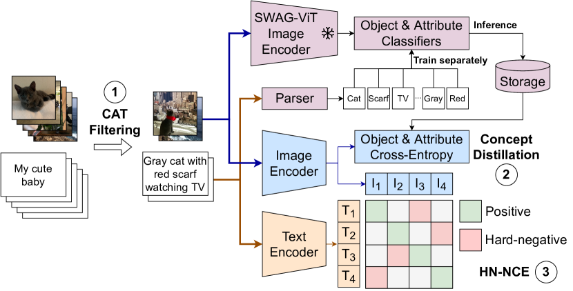
A summary of our pipeline is available in Figure 2. Our combined approach obtains significant improvements over the baseline for dual-encoder architectures on an elaborate benchmark of 29 tasks. Specifically, with the ViT-B/16 [17] architecture, we improve zero-shot performance on 20 out of 29 tasks, over CLIP training on the LAION-2B dataset [27, 66], despite training on a subset that is 80% smaller, see Figure 4. Furthermore, we demonstrate that even when trained with the smaller (but relatively less noisy) pretraining dataset PMD, our performance is better on 28 out of 29 tasks than CLIP trained on the same data, often with a large margin, see Figure 5.

Additionally, we present a simple yet effective approach to maintain the performance continuum as one moves from zero-shot to few-shot learning in the low data regime. Prior work [62] has shown a substantial drop in performance as one moves from zero-shot to $k$-shot learning, which is undesirable for practical scenarios. We propose an alternate linear probing approach that initializes the linear classifier with zero-shot text prompts and ensures that final weights do not drift away too much via projected gradient descent [5]. On ImageNet1K, we show huge improvements over prior work for small $k$ values. For example, our approach improves 5-shot top-1 accuracy by an absolute margin of 7% (see Figure 6) compared to the baseline strategy of linear probing with a random initialization.

Figure 2: Summary of our pipeline. We propose improvements to the standard vision-language pre-training: (1) Complexity, Action and Text-spotting (CAT) filtering that removes non-informative text-image pairs; (2) Concept distillation from a frozen (❄) pre-trained image encoder; (3) Hard-negative contrastive loss.

2 Related work

Dataset curation for contrastive pretraining.

Large-scale contrastive pretraining [11, 43, 62, 28, 41, 76, 85, 87] typically requires dataset sizes of the order of hundreds of millions to billions. Seminal works in this area, e.g., CLIP [62] and ALIGN [28], have largely relied on image-text pairs crawled from the web. Subsequently, versions of large-scale image-text datasets have been created but not released publicly, including WIT-400M [62], ALIGN-1.8B [28], FILIP-340M [85], FLD-900M [87], BASIC-6.6B [58], PaLI-10B [10]. These datasets often use unclear or primitive cleaning strategies, e.g., removing samples with short or non-English captions. Recently, LAION-400M [67] used CLIP-based scores to filter down a large dataset. The authors later released an English-only LAION-2B and a LAION-5B unfiltered dataset sourced from Common Crawl. Apart from LAION-400M and BLIP [40] which uses the bootstrapped image-grounded text encoder to filter out noisy captions, there has not been a significant investment in systematic curation strategies to improve zero-shot alignment performance on large-scale pretraining. In contrast to the previous work, we use quality-motivated filters that retain images whose captions are sufficiently complex, contain semantic concepts (actions), and do not contain text that can be spotted in the image [38].

Distillation from pre-trained visual models.

Knowledge distillation [25] aims to transfer knowledge from one model to another and has been used in many contexts ranging from improving performance and efficiency [6, 7, 42, 64, 81, 74, 68] to improving generalization capabilities [16, 44, 43]. Several approaches use self-distillation to improve performance with lower computational overhead [23, 82, 88]. For vision and language pre-training, [2, 41, 31] use soft-labels computed using embeddings from a moving average momentum model with the goal to reduce the adverse effects of noisy image-text pairs in the training data. Our concept distillation approach is a cheaper and more effective alternative, since it does not require us to run the expensive teacher model throughout the training while retaining the most useful information from the visual concepts.

Another approach to take advantage of pre-trained visual models is to use them to initialize the image encoder, and continue pre-training either by locking the image encoder [58, 89] or fine-tuning [58]. However, these approaches lack the ability to align complex text to a fully-trained image encoder, and thus perform poorly on multimodal tasks, e.g. cross-modal retrieval (see Section 4.3).

Contrastive training with hard negatives.

Noise-contrastive estimation (NCE) [22] is the typical objective for vision-text learning, with applications across large-scale multimodal alignment [62, 28, 11, 43] and unsupervised visual representation learning [53, 24]. Several lines of work have studied the shortcomings of the original InfoNCE objective [55], specifically, the selection and importance of negative samples. Chuang et al. [12] present a debiasing approach to account for false negatives at very large batch sizes, typical in large-scale pretraining. Kalantidis et al. [30] present a MixUp approach to improve the quality of hard negative samples for unsupervised alignment. Using model-specific hard negatives in the training objective is proven to reduce the estimation bias of the model as well [90]. Contrary to prior semi-supervised work, we extend the model-based hard negative objective, first proposed in Robinson et al. [63] to multimodal alignment.

3 Method

Background.

We consider the task of contrastive image-text pretraining. Given a dataset $𝒟={\{(I_i,T_i)\}}_{i=1}^N$ of image-text pairs, we want to learn a dual encoder model $\mathit{\varphi }=\{{\mathit{\varphi }}_{\text{image}},{\mathit{\varphi }}_{\text{text}}\}$, where ${\mathit{\varphi }}_{\text{image}}$ represents the image encoder, and ${\mathit{\varphi }}_{\text{text}}$ denotes the text encoder. We use the shorthand $𝒙={\mathit{\varphi }}_{\text{image}}(I)$ and $𝒕={\mathit{\varphi }}_{\text{text}}(T)$ to denote the encoded images and texts, respectively, for an image-text pair $(I,T)$. We will now describe the three crucial components of our approach followed by the final training objective.

3.1 Complexity, Action, and Text (CAT) filtering

Our complexity, action, and text spotting (CAT) filtering is a combination of two filters: a caption complexity filter that removes image-caption pairs if a caption is not sufficiently complex, and an image filter that removes pairs if the image contains text matching the caption to prevent polysemy during alignment. We use the LAION-2B pre-cleaned obtained after using filters in [69] as the base dataset.

Filtering captions via complexity & actions.

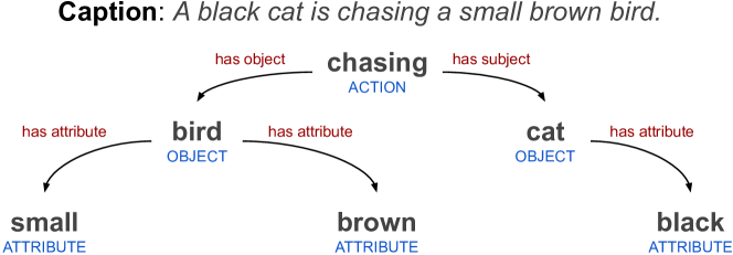
Noisy web-scale datasets do not have any semantic-based curation, and hence captions can be irrelevant, ungrammatical and unaligned. Our motivation is to decrease such noise by simply selecting captions that possess sufficient complexity, so that the training distribution matches the target tasks. To this end, we build a fast rule-based parser that extracts objects, attributes and action relations (see Figure 3 for an example) from text and we use the resulting semantic graph to estimate the complexity of the image captions. Specifically, we define the complexity of a caption as the maximum number of relations to any object present in the parse graph. For example, in the caption “A black cat is chasing a small brown bird,” the object “bird” has the attributes “small”, “brown” and “A black cat is chasing”, and hence, the complexity of the caption is C$3$. We only retain samples that at least have a C$1$ caption complexity. To further remove pairs likely containing products, we filter out captions if they do not contain at least one action (as obtained from the parser).

Figure 3: An example caption and its parse. The caption has C$3$ complexity (due to bird) and has 1 action (chasing).

Filtering images via text-spotting.

Image-caption pairs in web-scale datasets often display part of the caption as text in the image (on visual inspection, we found up to $\sim$30% such examples for LAION [66]). Minimizing the objective, in these cases, can correspond to spotting text (e.g., optical character recognition) rather than the high-level visual semantics (e.g., objects, attributes) we would like the model to align to. This will reduce performance on object-centric and scene-centric downstream zero-shot tasks, and hence we remove such images from the training set using an off-the-shelf text spotter [38]. We remove image-text pairs with a text spotting confidence of at least $0.8$ and at least $5$ predicted characters matching the caption in a sliding window. We observe (by inspection) that this approach is efficient at identifying images with text, and failure cases are primarily in non-English text. Filtering with multilingual text spotters trained can fix this issue, however, we leave this as future work. Filtering statistics can be found in the supplement.

3.2 Concept distillation

Recognizing visual concepts in images that correspond to objects and attributes in corresponding captions is crucial for alignment. We therefore propose to distill these concepts from a pre-trained teacher model to our image encoder. Specifically, we add two auxiliary linear classifiers on top of the encoded image embeddings $𝒙$ to predict (i) objects and (ii) visual attributes and use the teacher model to generate the pseudo-labels for training them. These classifiers are trained jointly with the contrastive loss.

We parse image captions using a semantic parser that extracts objects and attributes from text (Section 3.1) and use these as pseudo-labels. We then train the linear classifiers on the teacher model embeddings with a soft-target cross-entropy loss [20], after square-root upsampling low-frequency concepts [49]. It is important to freeze the backbone of the teacher model to make sure we retain the advantages of using a stronger model for distillation. For each image, we then use these trained linear classifiers to generate two softmax probability vectors – ${𝒑}^{\text{obj}}$ for objects, and ${𝒑}^{\text{attr}}$ for attributes, respectively. To minimize the storage overhead, we further sparsify them by retaining only the top-$k$ predicted class values and re-normalizing them to generate the final pseudo-labels. During multimodal training, we use the cross-entropy loss with these pseudo-label vectors as targets. Unless specified otherwise, we use the ViT-H/14 [17] architecture pretrained from SWAG [71] as the teacher model. See Section 4.2 and the supplementary material for ablations on the effect of different backbones and retaining top-$k$ predictions, and further details.

There are several advantages of our concept distillation approach. First, the teacher predictions capture correlations from the strong vision encoding, making them more informative as labels compared to the captions themselves. The captions are limited to a few objects and attributes, while the teacher predictions yield a more exhaustive list. Moreover, our approach reaps the benefits of the recently proposed and publicly-available strong unimodal vision models more effectively than other distillation approaches, as training linear classifiers on a frozen teacher model is inexpensive. After predictions are stored, we discard the teacher model and thus bypass the memory and compute limitations of simultaneously running the student and teacher model in standard distillation approaches [25, 74], which is critical for large teacher models. We demonstrate empirically (see Section 4.2) that our strategy works better than distilling teacher embeddings directly. Additionally, compared to approaches that warm-start the image encoder with pre-trained models, our method can leverage higher capacity teacher models without difficulty and unlike locked-image tuning [58, 89], our approach gives the flexibility of training the image encoder for better alignment, while retaining the strength of the pre-trained visual features.

3.3 Multimodal alignment with hard negatives

Contrastive learning [55] has quickly become the de-facto approach for multimodal alignment, where most prior work focuses on the multimodal InfoNCE [55] objective, given for any batch $𝐗={\{({𝒙}_i,{𝒕}_i)\}}_{i=1}^n$ of featurized image-text pairs as (for some learnable temperature $\tau >0$),

${ℒ}_{\text{NCE}}\left(𝐗\right)=-{\displaystyle \sum _{i=1}^n}\left[\log {\displaystyle \frac{e^{{𝒙}_i^{\top }{𝒕}_i/\tau }}{{\sum }_j{e}^{{𝒙}_i^{\top }{𝒕}_j/\tau }}}+\log {\displaystyle \frac{e^{{𝒙}_i^{\top }{𝒕}_i/\tau }}{{\sum }_j{e}^{{𝒙}_j^{\top }{𝒕}_i/\tau }}}\right].$

While this approach has enjoyed immense success in multimodal alignment [62, 28], when learning from large-scale noisy datasets, uniform sampling as applied in noise-contrastive estimation can often provide negative samples that are not necessarily discriminative, necessitating very large batch sizes. For the problem of contrastive self-supervised learning, Robinson et al. [63] propose an importance-sampling approach to reweight negative samples within a batch so that “harder” negatives are up-sampled in proportion to their difficulty. We present a similar strategy for multimodal alignment. Specifically, for some $\alpha \in (0,1],\beta \ge 0$, we propose the following hard-negative noise contrastive multimodal alignment objective:

${ℒ}_{\text{HN-NCE}}\left(𝐗\right)=-$ ${\displaystyle \sum _{i=1}^n}\log \left[{\displaystyle \frac{e^{{𝒙}_i^{\top }{𝒕}_i/\tau }}{\alpha \cdot e^{{𝒙}_i^{\top }{𝒕}_i/\tau }+\sum _{j\ne i}{e}^{{𝒙}_i^{\top }{𝒕}_j/\tau }{w}_{{𝒙}_i,{𝒕}_j}^{i\to t}}}\right]$

$-$ ${\displaystyle \sum _{i=1}^n}\log \left[{\displaystyle \frac{e^{{𝒙}_i^{\top }{𝒕}_i/\tau }}{\alpha \cdot e^{{𝒙}_i^{\top }{𝒕}_i/\tau }+\sum _{j\ne i}{e}^{{𝒙}_j^{\top }{𝒕}_i/\tau }{w}_{{𝒙}_j,{𝒕}_i}^{t\to i}}}\right].$

Where the weighing functions are given as:

$w_{{𝒙}_i,{𝒕}_j}^{i\to t}={\displaystyle \frac{\left(n-1\right)\cdot e^{\beta {𝒙}_i^{\top }{𝒕}_j/\tau }}{{\sum }_{k\ne i}{e}^{\beta {𝒙}_i^{\top }{𝒕}_k/\tau }}},w_{{𝒙}_j,{𝒕}_i}^{t\to i}={\displaystyle \frac{\left(n-1\right)\cdot e^{\beta {𝒙}_j^{\top }{𝒕}_i/\tau }}{{\sum }_{k\ne i}{e}^{\beta {𝒙}_k^{\top }{𝒕}_i/\tau }}}.$

The weights $w_{\beta }$ are designed such that difficult negative pairs (with higher similarity) are emphasized, and easier pairs are ignored. Furthermore, $\alpha$ rescales the normalization with the positive terms to account for the case when false negatives are present within the data. The form of weights $w_{\beta }$ is an unnormalized von Mises-Fisher distribution [50] with concentration parameter $\beta$. Observe that we obtain the original objective when setting $\alpha =1$ and $\beta =0$. There are several key differences with the original formulation of [63] and the HN-NCE objective presented above. First, we utilize only cross-modal alignment terms, instead of the unimodal objective presented in [63]. Next, we employ separate penalties for text-to-image and image-to-text alignment. Finally, we incorporate a learnable temperature parameter $\tau$ to assist in the learning process. We discuss our design choices in more detail with additional theoretical and experimental justifications in the supplementary material.

3.4 Training objective

For any batch $𝐗=\{{({𝒙}_i,{𝒕}_i)}_{i=1}^n\}$ of $n$ image-text pairs, we minimize the following objective:

${ℒ}_{\text{HN-NCE}}(𝐗)+{ℒ}_{\text{CE-O}}(𝐗)+{ℒ}_{\text{CE-A}}(𝐗),\text{where,}$

${ℒ}_{\text{CE-O}}(𝐗)={\displaystyle \sum _{i=1}^n}\text{Cross-Entropy}({𝒑}_i^{\text{obj}},f_{\text{obj}}({𝒙}_i)),\text{and,}$

${ℒ}_{\text{CE-A}}(𝐗)={\displaystyle \sum _{i=1}^n}\text{Cross-Entropy}({𝒑}_i^{\text{attr}},f_{\text{attr}}({𝒙}_i)).$

Here, both $f_{\text{obj}}$ and $f_{\text{attr}}$ are linear classifiers, the vectors ${𝒑}^{\text{obj}},{𝒑}^{\text{attr}}$ are the top-k predicted objects and attributes from the teacher model (Section 3.2), and ${ℒ}_{\text{hn-nce}}$ is the hard-negative contrastive alignment loss (Section 3.3).

4 Experiments

Here we evaluate our approach across a broad range of vision and vision-language tasks. We provide extensive ablations on 29 tasks over the design choices in Section 4.2, and compare with state-of-the-art approaches on popular zero-shot benchmarks in Section 4.3. Finally, we present an alternate approach to do few-shot classification with prompt-based initialization in Section 4.4.

4.1 Experimental setup

Training datasets.

We use a 2.1B English caption subset of the LAION-5B dataset [66]. Prior to training, we filter out sample pairs with NSFW images, toxic words in the text, or images with a watermark probability larger than $0.5$, following [69]. This leaves us with 1.98B images, which we refer to throughout the paper as the LAION-2B dataset. Additionally, we explore training our models on a collection of Public Multimodal Datasets (PMD) from [70]. PMD contains training splits of various public datasets. After downloading the data we are left with 63M (vs. 70M reported in [70]) image-text pairs due to missing samples and SBU Captions [56] (originally in PMD) going offline.

Training details.

For our model architecture, we closely follow CLIP by Radford et al. [62]. We utilize Vision Transformers (ViT) [17] for images and Text Transformers [75] for captions. We experiment with 3 different architectures, denoted as B/32, B/16, and L/14, where 32, 16, and 14 denote the input image patch size. See the supplementary for architecture details. For distillation and fine-tuning experiments, we utilize the public SWAG-ViT models [71], pre-trained with weak supervision from hashtags.

We use the Adam [33] optimizer with a decoupled weight decay [48] and a cosine learning rate schedule [47]. The input image size is 224$\times$224 pixels. To accelerate training and save memory, we use mixed-precision training [51]. All hyperparameters are presented in the supplementary. They are selected by training B/32 on a small scale setup, and reused for all architectures. For objects and attributes classifiers, we found that scaling the learning rate by 10.0 and weight decay by 0.01 gave better results. We train our models on 4B, 8B, 16B, and 32B total samples. For ViT-L/14, we further train the model at a higher 336px resolution for 400M samples, denoting this model as L/14@336. We trained L/14 for 6 days on 512 A100 GPUs with 16B processed samples for a total of $7.4\times {10}^4$ GPU hours.

Evaluation benchmarks.

We evaluate our models on a zero-shot benchmark of 29 tasks: (i) 17 image classification, (ii) 10 cross-modal retrieval, (iii) 2 visual question answering. Dataset details are presented in the supplement.

4.2 Ablations on zero-shot benchmarks

In this section, we ablate our three pretraining contributions: dataset filtering, distillation from objects and attributes predictions, and, hard negative contrastive objective. Ablations are performed over zero-shot Accuracy@1 on the ImageNet1K [65] (IN) validation set, text-to-image (T2I) and image-to-text (I2T) zero-shot Recall@1 on the COCO [60] and Flickr [59] test sets. We also report the change in accuracy (%) over 29 zero-shot tasks between our model and baselines. For a fair comparison, we train all approaches presented in this section (including baselines).

Effect of dataset filtering.

We apply our filters, as well as filtering based on CLIP [62] alignment score (0.35), and ablate the baseline performance, without distillation or hard negative contrastive training, in Table 1 for ViT-B/32 model architecture. All models see 4B total samples during training, while the number of unique samples drops after each filtering step. Complexity filter (C) in row (3) reduces the dataset size by around 270M, while slightly increasing image-text alignment as observed on T2I task. Next, action filter (A) in row (4) reduces the size by more than 1B, while it has a large benefit in aligning complex text. However, as expected, it hurts performance on object-centric ImageNet. Finally, text-spotting (T) filter in row (5) boosts alignment across the board, due to the fact that it removes the need to learn a bimodal visual representation of the text. We also compare with filtering based on CLIP score in row (2), which was selected such that the dataset size is comparable to ours, and show that it is too strict and removes plenty of useful training pairs, thus hurting the performance. Finally, LAION-CAT, with only 22% of the original dataset size, significantly boosts image-text zero-shot performance. We also observed that gains hold as we train for longer training schedules. See the supplementary for details.

Table 1: Evaluating effect of using LAION-2B subset filtered on complexity (C), actions (A), and text-spotting (T). CLIP denotes filtering pairs with CLIP score bellow 0.35. Evaluation performed on ViT-B/32 model architecture trained for 4B processed samples.

#	Filter				Size	IN	COCO		Flickr
	CLIP	C	A	T			T2I	I2T	T2I	I2T
1					1.98B	60.8	33.7	52.1	59.3	77.7
2	✓				440M	52.5	29.8	46.1	54.8	72.0
3		✓			1.71B	60.8	33.9	52.5	60.8	77.8
4		✓	✓		642M	58.7	35.9	53.8	64.3	82.0
5		✓	✓	✓	438M	61.5	37.6	55.9	66.5	83.2

Effect of distillation approach.

To understand the effect of direct distillation from a pre-trained SWAG-ViT visual encoder [71], we investigate two baseline approaches:

(1) Embedding distillation (ED) borrows from SimSiam [9] and uses an auxiliary negative cosine similarity loss between the image representation from the student visual encoder and the pre-trained SWAG model.
(2) Distribution distillation (DD) borrows ideas from momentum distillation in ALBEF [41] and computes the cross-modal similarities between the SWAG image representation and the student text representation and uses them as soft-labels for student image representation and text alignment. The soft-labels are linearly combined with the hard $0-1$ labels before applying the InfoNCE [55] loss.

A comparison of our distillation from predicted concepts (CD) with the aforementioned distillation approaches is presented in Table 2 (upper section). Note that for a fair comparison, we do not use our hard-negative contrastive loss for these experiments. Our distillation approach performs the best, even though it has virtually no training overhead as the predicted concepts are pre-computed, while, e.g., ED is 60% slower with an 8% increase in GPU memory due to the need of running an additional copy of the vision tower. One could pre-compute embeddings for ED and DD as well, but that increases dataset size by 1.2TB and creates a data loading bottleneck, while our pre-computed predictions take only 32.6GB additional storage space when saving the top-10 predictions (see supplementary). We additionally show that our approach is robust to the number of top-$k$ predictions used, details in the supplementary.

One could also use an external unimodal image model and fine-tune it on the image-text alignment task instead of using distillation. We follow [89] and explore three fine-tuning options as baselines: (i) locked-image tuning (LiT) where the image encoder is locked, and only the text encoder is trained, (ii) fine-tuning (FT) where the image encoder is trained with a learning rate scaled by 0.01 compared to the text encoder, (iii) fine-tuning with delay (FT-delay) where the image encoder is locked for half of the pre-training epochs following (i), and then fine-tuned for the rest following (ii). Results of these setups are ablated in Table 2 (lower section). LiT vs. FT is a trade-off between strong performance on image recognition tasks (as measured with ImageNet1K) and better image-text alignment (as measured by COCO and Flickr). Locking the image encoder makes the alignment very hard to achieve, but fine-tuning it hurts its original image recognition power. On the other hand, we show that our concept distillation is the best of both worlds, it surpasses LiT or FT in 4 out of 5 metrics. Another drawback of FT is that it requires the same architecture in the final setup, while CD can be effortlessly combined with any architecture or training setup, by using stored predictions as metadata. To conclude, unlike related approaches, our proposed distillation: (i) has almost no cost at training, (ii) is architecture agnostic, (iii) improves both image recognition and complex image-text alignment.

Table 2: Evaluating effect of using different initialization or distillation approaches. Evaluation performed on ViT-B/16 model architecture trained for 16B processed samples on LAION-CAT. Init: Initialization with random or SWAG-B/16 weights. ED: Embedding distillation. DD: Distribution distillation. LiT: Locked image tuning. FT: Fine-tuning. FT-delay: Locked image tuning for 50% followed by fine-tuning for the rest. CD: Our concept distillation using teacher-predicted objects and attributes.

Init	Method	SWAG	IN	COCO		Flickr
		(teacher)		T2I	I2T	T2I	I2T
Random	Baseline	—	68.7	42.8	60.5	72.8	89.7
	ED	B/16	69.2	42.6	59.4	72.8	86.8
	DD	B/16	68.6	41.8	57.4	71.7	87.0
	CD (ours)	B/16	71.0	42.8	59.5	72.3	86.5
	CD (ours)	H/14	72.3	43.4	60.4	73.8	87.6
SWAG	LiT	—	73.0	32.5	50.6	60.8	79.6
	FT	—	71.2	43.1	60.3	73.1	87.7
	FT-delay	—	72.0	42.7	60.7	72.5	86.2

Effect of hard negative contrastive training.

We present the ablation when using hard negative contrastive objective (HN-NCE) in Table 3. Performance suggests that using the newly proposed loss is beneficial compared to the vanilla InfoNCE, and that its positive effects are complementary to the gains from the proposed distillation from objects and attributes predictions. Please see the supplementary for ablations on the effect of the hyperparameters $\alpha$ and $\beta$.

Table 3: Evaluating effect of using hard negative contrastive loss. Evaluation performed on ViT-B/16 model architecture trained for 16B processed samples on LAION-CAT. CD: Our concept distillation using SWAG-H/14 predicted objects and attributes. HN: Our proposed hard negative contrastive loss.

#	Method		IN	COCO		Flickr
	CD	HN		T2I	I2T	T2I	I2T
1			68.7	42.8	60.5	72.8	89.7
2	✓		72.3	43.4	60.4	73.8	87.6
3	✓	✓	72.0	43.7	62.0	73.2	89.5

Effect when pre-training on PMD.

Finally, we analyze our proposed recipes when training visual-language models on a much smaller dataset, i.e. PMD with 63M training samples. Results are shown in Table 4. All contributions improve the performance over baseline significantly, hence we conclude that using the proposed pipeline is very beneficial in low-resource training regimes. Note that, the PMD dataset contains COCO and Flickr training samples, hence, it is not strictly zero-shot evaluation. For that reason, we do not compare our models trained on PMD dataset with state-of-the-art models in the following section. However, we believe these strong findings will motivate usage of our approach on smaller and cleaner datasets, as well.

Table 4: Evaluating effect when pre-training on PMD using our approaches. Evaluation performed on ViT-B/32 and ViT-B/16 models trained for 4B processed samples. CD: Our concept distillation using SWAG-H/14 predicted objects (-O) and attributes (-A). HN: Our proposed hard negative contrastive loss.

Arch.	#	Method			IN	COCO		Flickr
		CD-O	CD-A	HN		T2I	I2T	T2I	I2T
B/32	1				49.0	28.9	50.2	62.0	80.3
	2	✓			57.8	32.2	54.0	65.6	85.7
	3	✓	✓		59.7	34.4	55.7	68.3	87.8
	4	✓	✓	✓	62.4	37.3	60.4	71.8	89.9
B/16	5				54.6	33.1	55.7	67.4	85.5
	6	✓	✓		65.5	37.4	59.9	72.4	88.7
	7	✓	✓	✓	67.8	42.7	65.5	77.6	92.5

Zero-shot benchmarks.

We denote model trained with our proposed concept distillation and hard-negative loss as DiHT. To showcase our model’s performance in more detail, we report our DiHT-B/16 trained on LAION-CAT with 438M samples vs. CLIP-B/16 baseline trained by us on LAION-2B with 2B samples in Figure 4. Additionally, we report DiHT-B/16 vs. CLIP-B/16 baseline, where both models are trained on PMD dataset with 63M samples in Figure 5. When trained on LAION-CAT or LAION-2B, respectively, DiHT wins on 20 out of 29 benchmark tasks. Impressively, when trained on PMD, DiHT wins on 28 out of 29 benchmarks tasks, usually with a very large margin.

Figure 4: DiHT-B/16 trained on LAION-CAT with 438M samples vs. CLIP-B/16 trained on LAION-2B with 2B samples. Both models trained by us with 32B total processed samples.

Figure 5: DiHT-B/16 vs. CLIP-B/16. Both models trained by us on PMD with 63M images and 4B total processed samples.

Robustness to distribution shift.

We evaluate the ImageNet-related robustness on different datasets in Table 5, for DiHT-B/16 vs. CLIP-B/16 baseline, trained by us on PMD and LAION datasets. Our proposed approach improves on robustness over vanilla CLIP, in some cases by a significant margin, e.g. ImageNet-A and ObjectNet.

Table 5: ImageNet robustness performance on ViT-B/16 models.

Method	Train Data	#D	IN	IN-V2	IN-A	IN-R	IN-Sketch	ObjectNet
CLIP	PMD	63M	54.6	47.9	35.5	56.3	30.8	38.5
DiHT	PMD	63M	67.8	61.5	54.3	74.4	44.7	52.8
CLIP	LAION-2B	1.98B	70.3	62.7	39.3	81.0	57.1	56.2
DiHT	LAION-CAT	438M	72.2	64.3	49.2	85.1	58.3	62.3

4.3 Comparison with zero-shot state of the art

We compare our DiHT models against state-of-the-art dual-encoder models in Table 6. Given that all models use different architectures, input image resolutions, training databases, and number of processed samples at training, we outline those details in the table, for easier comparison.

Our approach is most similar to CLIP [62] and OpenCLIP [27], and has same training complexity and inference complexity. We outperform models with same architecture by substantial margins, even when our training dataset is much smaller. Our best models DiHT-L/14 and DiHT-L/14@336 trained at higher $336$px resolution for additional 400M samples outperform models with significantly more complexity on popular text-image COCO and Flickr benchmarks. Compared to ALIGN [28] that has approximately twice the number of parameters compared to our DiHT-L/14 model and is trained on 4x bigger data, we improve the performance substantially for all the retrieval benchmarks. Our model also performs better than FILIP [85] which utilizes token-wise similarity to compute the final alignment, thus noticeably increasing the training speed and memory cost. We also outperform Florence [87] on all $4$ retrieval benchmarks. Note that Florence [87] utilizes a more recent and powerful Swin-H Vision Transformer architecture [46] with convolutional embeddings [78], and a unified contrastive objective [84]. Our proposed contributions are complementary to FILIP [85] and Florence [87], and we believe additional gains can be achieved when combined. Finally, LiT [89] and BASIC [58] first pre-train model on an large-scale image annotation dataset with cross-entropy before further training with contrastive loss on an image-text dataset. Though this strategy results in state-of-the-art performance on ImageNet1K [65] and image classification benchmarks, it has severe downsides on multi-modal tasks such as cross-modal retrieval. Our ablation in Section 4.2 also confirms this issue. On the other hand, our approach does not suffer from such negative effects.

Table 6: Comparison with zero-shot state-of-the-art dual-encoder models. px: input image size; #P: model size; #D: training dataset size; #S: total samples processed at training. We evaluate CLIP [62] and OpenCLIP [27] using our codebase, other numbers are copied from respective papers. Grouped models (e.g., ViT-B/32) share same vision and language architecture as our model, following CLIP [62], others have different architectures and we outline the vision one. ^∗FILIP uses token-wise similarity, which is more expensive than global-token similarity and requires adapting the architecture, hence we put it in “Other”.

Method	px	#P	#D	#S	IN	COCO		Flickr
						T2I	I2T	T2I	I2T
ViT-B/32
CLIP [62]	224	151M	400M	12.8B	63.4	31.4	49.0	59.5	79.9
OpenCLIP [27]	224	151M	400M	12.8B	62.9	34.8	52.3	61.7	79.2
OpenCLIP [27]	224	151M	2.3B	34B	66.6	39.0	56.7	65.7	81.7
DiHT	224	151M	438M	16B	67.5	40.3	56.3	67.9	83.8
DiHT	224	151M	438M	32B	68.0	40.6	59.3	68.6	84.4
ViT-B/16
CLIP [62]	224	150M	400M	12.8B	68.4	33.7	51.3	63.3	81.9
OpenCLIP [27]	224	150M	400M	12.8B	67.1	37.8	55.4	65.2	84.1
OpenCLIP [27]	240	150M	400M	12.8B	69.2	40.5	57.8	67.7	85.3
DiHT	224	150M	438M	16B	71.9	43.7	62.0	73.2	89.5
DiHT	224	150M	438M	32B	72.2	43.3	60.3	72.9	89.8
ViT-L/14
CLIP [62]	224	428M	400M	12.8B	75.6	36.5	54.9	66.1	84.5
CLIP [62]	336	428M	400M	13.2B	76.6	37.7	57.1	68.6	86.6
OpenCLIP [27]	224	428M	400M	12.8B	72.8	42.1	60.1	70.4	86.8
OpenCLIP [27]	224	428M	2.3B	32B	75.2	46.2	64.3	75.4	90.4
DiHT	224	428M	438M	16B	77.0	48.0	65.1	76.7	92.0
DiHT	336	428M	438M	16.4B	77.9	49.3	65.3	78.2	91.1
Other
ALIGN [28] EfficientNet-L2	289	820M	1.8B	19.7B	76.4	45.6	58.6	75.7	88.6
FILIP [85]∗ ViT-L/14	224	428M	340M	10.2B	77.1	45.9	61.3	75.0	89.8
OpenCLIP [27] ViT-H/14	224	986M	2.3B	32B	77.9	49.0	67.5	76.8	91.3
Florence [87] CoSwin-H	384	893M	900M	31B	83.7	47.2	64.7	76.7	90.9
LiT [89] ViT-g/14	288	2.0B	3.6B	18.2B	85.2	41.9	59.3	—	—
BASIC [58] CoAtNet-7	224	3.1B	6.6B	32.8B	85.7	—	—	—	—

4.4 Few-shot linear probing

The ideal scenario for leveraging zero-shot recognition models is to warm start the task without training data and then improve the performance (by training a linear probe) via few-shot learning as more and more data is seen. However, in practice, few-shot models perform significantly worse than zero-shot models in the low-data regime.

We present an alternate approach to do few-shot classification with prompt-based initialization. The key idea of our approach is to initialize the classifier with the zero-shot text prompts for each class, but to also ensure that the final weights do not drift much from the prompt using projected gradient descent (PGD) [5]. While few-shot models have been initialized with prompt priors in the past with naive $L_2$ penalties for weight to prevent catastrophic forgetting [34], these approaches do not improve performance and the model simply ignores the supervision. In contrast, for any target dataset ${𝒟}_{\text{target}}=\{{({𝒙}_i,y_i)}_{i=1}^n\}$, where ${𝒙}_i={\mathit{\varphi }}_{\text{image}}(I_i)$ denotes the image features from the trained image tower, we solve the following optimization problem, for some $\delta ,{\delta }_b>0$:

$$\underset{{\parallel 𝐖\parallel }_2\le \delta ,{\parallel 𝒃\parallel }_2\le {\delta }_b}{\min }\sum _{i=1}^n{ℒ}_{\text{CE}}(y_i,{𝒙}_i^{\top }\left(𝐖+{𝐖}_{\text{0}}\right)+𝒃).$$

Here ${𝐖}_0\in {ℝ}^{d\times n_c}$ denotes the prompt initialization from the text encoder. To optimize the objective, one can use projected gradient descent [5]. We observe that our approach is able to bridge the gap between zero-shot and 1-shot classification, a common issue in prior linear probe evaluations.

Figure 6 presents the full summary of results on the ImageNet1K [65] $k$-shot classification task. Hyperparameters $\delta$ and ${\delta }_b$ for our approach, and weight decay for the baseline approach of training linear probes from scratch are found using grid search. Note that compared to the baseline, our method performs substantially better at very low values of $k$ and maintains the performance continuum from zero-shot to 1-shot, and so on. At large $k$ values, both approaches perform similarly, since there are sufficient data samples to render the zero-shot initialization ineffective. To further showcase the strength of our approach, we also compare our performance with linear probes trained on powerful SWAG [71] models that are especially suited for this task. Note that our approach outperforms the much larger SWAG ViT-H/14 model up to 25-shot classification. We would like to emphasize that this albeit straightforward approach is one of the first to resolve this discontinuity problem between zero-shot and few-shot learning.

Figure 6: $k$-shot linear probing performance on ImageNet1K.

5 Conclusion and future work

In this paper, we demonstrate that with careful dataset filtering and simple but effective modeling changes, it is possible to achieve substantial improvements in zero-shot performance on retrieval and classification tasks through large-scale pre-training. Our CAT filtering approach can be applied generically to any large-scale dataset for improved performance with smaller training schedules. Moreover, our concept distillation approach presents a compute and storage efficient way of leveraging very large capacity pre-trained image models for multimodal training. Finally, our simple projected gradient approach covers the crucial performance gap between zero-shot and few-shot learning.

In future, we would like to extend our approach to multi-modal encoder/decoder [1, 86, 10, 41, 83] architectures that although expensive, have better zero-shot performance compared to dual encoders. We also observe that benefits of our hard-negatives loss are less on noisier LAION dataset compared to PMD. It would be interesting to explore how to make it more effective in these very noisy settings. We hope that our improvements and extensive large-scale ablations will further advance the vision-language research.

Appendix A Appendix

A.1 Method details

A.1.1 Semantic parser

To enable a rich complexity and semantic filtering, we built a fast custom semantic parser that converts a given textual caption to a semantic graph similar to the one in Visual Genome[36]. In particular, we extract objects, their parts, their attributes, and the actions that they are involved in (see Figure 3 for example). The parser is built on top of the English language dependency parser from Spacy[26] combined with multiple rules to infer common object relations. The aim of the parser is high speed with high precision of common object relations such as ‘has_attribute‘ and ‘has_part‘ and basic ‘action‘ support. Below, we describe the structured relations that we extract from natural language text.

We support the following semantic relations:

Object (_obj).

We extract objects that are supposedly presented in an image. We consider nouns that are not attributes of another noun (not part of a noun phrase). E.g. in birthday cake and baby stroller, the nouns cake and stroller are parsed as objects, and the nouns birthday and baby are considered attributes. We do not consider proper nouns.

Attribute (has_attr).

Denotes attributes that characterize an object or another attribute. For example, dark green, would result in a fact green - has_attr - dark, and yellow candles results in candles - has_attr - yellow.

Part (has_part).

Characterizes a visual part of an object. E.g. cake with 21 yellow candles would result in a part fact cake - has_part - candles.

Action (_act).

Verbs that do not entail attributes or parts (e.g. forms of be, looks, seems, and have are excluded) are considered actions. For actions, we also parse the subject and object arguments.

Subject of an action (act_has_subj, is_act_subj).

We use the act_has_subj and is_act_subj relation to represent arguments (nouns) that are the subject of an action. E.g. for the text a person is eating an apple, we add the object-centric and corresponding action-centric symmetric facts: person - is_subj_act - eating and eating act_has_subj person.

Object of an action (act_has_obj, is_act_obj).

We also include the relations that specify the object arguments of an action. E.g. for the text a person is eating an apple, we add the object-centric and corresponding action-centric symmetric facts: apple - is_obj_act - eating and eating act_has_obj apple.

We recognize the following limitations of ours approach:

Semantic attributes.

In this work, we focus on object-centric visual and action characteristics and we do not process spatial relations ( X next to Y) or additional action arguments (read a book *in* the library). Spatial relations and additional arguments of verbs usually involve more complex semantic reasoning and require more robust approaches and task-specific models such as one trained on Semantic Role Labeling which are usually compute-heavy. We leave these for future work.

Dependency parser errors.

In the current version of the parser, we also parse potential attributes as actions, which are not likely to be always visual. E.g. In the phrase “running person”, running is an action and an attribute, and we parse them as such. However, sometimes the underlying parser would also parse attributes in phrases such as “striped mug” as verbs, where we process the attribute “striped” as both an attribute and an action (without arguments).

A.1.2 Concept distillation

The teacher model is built by training linear classifiers - which predict objects and attributes - on top of a frozen SWAG [71] backbone. SWAG is trained in a weakly-supervised manner by predicting hashtags from Instagram images. We use the publicly available weights, and adopt a training procedure that is similar to the one from SWAG for learning the linear classifiers. The procedure for training the object classifier is as follows. First, we parse the captions to extract nouns. Next, we canonicalize the nouns via WordNet [52] synsets and remove ones which occur less than 250 times in the dataset. The resulting vocabulary contains $\sim$10K unique synsets. Finally, we optimize the linear layer’s weights through a cross-entropy loss. Each entry in the target distribution of the cross-entropy is either $1/K$ or $0$ depending on whether the corresponding synset is present or not, where $K$ is the number of synsets for that image. We apply inverse square-root resampling of images to upsample the tail classes following [71]. The target length of the dataset is set to 50 million samples during resampling . We train the linear layer using SGD with momentum 0.9 and weight decay 1e-4. The learning rate is set following the linear scaling rule: lr$=$0.001$\cdot$$\frac{bs}{256}$. To speedup training, we use 64 GPUs with batch size of 256 per GPU. The attribute classifiers are build in a similar way, but the WordNet adjective synsets require additional filtering to remove non-visual attributes, e.g., claustrophobic, experienced. Following [61], we select the attributes based on their sharedness and visualness. We rank the attributes based on the aforementioned scores, and keep $\sim$1200 attributes.

A.2 Training details

For our model architecture, we closely follow CLIP by Radford et al. [62]. We utilize Vision Transformers (ViT) [17] for images and Text Transformers [75] for captions. We experiment with 3 different architectures, denoted as B/32, B/16, and L/14, where 32, 16, and 14 denote the input image patch size. Other architecture scaling parameters are in Table A.1. For distillation and fine-tuning experiments, we utilize the public SWAG-ViT models [71], pre-trained with weak supervision from hashtags.

Table A.1: DiHT architecture hyperparameters.

Model	Dim	Vision			Language
		layers	width	heads	layers	width	heads
B/32	512	12	768	12	12	512	8
B/16	512	12	768	12	12	512	8
L/14	768	24	1024	16	12	768	12

We use the Adam [33] optimizer with a decoupled weight decay [48] and a cosine learning rate schedule [47]. Input image size is 224$\times$224 pixels, for pre-training runs. All hyperparameters are presented in Table A.2. They are selected by training on a small scale setup, and reused for other experiments. For objects and attributes classifiers in concept distillation (CD), we found that scaling the learning rate by 10.0 and weight decay by 0.01 gave better results.

Table A.2: DiHT common hyperparameters.

Shared
Learning rate (LR)	1e-3
Warm-up	1%
Vocabulary size	49408
Temperature (init, max)	($\frac{1}{0.07}$, 100.0)
Adam (${\beta }_1$, ${\beta }_2$)	(0.9, 0.98)
Adam $ϵ$	1e-6
High resolution LR	1e-4
Dataset specific	LAION		PMD
CD learning rate scale	10.0		1.0
CD weight decay scale	0.01		1.0
HN-NCE $\alpha$	1.0		0.999
HN-NCE $\beta$	0.25		0.5
	LAION		PMD
Model specific	L/14	B/16,B/32	B/16,B/32
Batch size	98304	49152	32768
Weight decay	0.2	0.1	0.1

We pre-train the models on 4B, 8B, 16B, or 32B processed samples, depending on the experiment. For L/14 we train at a higher 336px resolution for additional 400M samples, denoting this models as L/14@336. We trained L/14 for 6 days on 512 A100 GPUs with 16B processed samples for a total of $7.4\times {10}^4$ GPU hours.

To accelerate training and save memory, we use mixed-precision training [51]. For L/14 we use grad checkpointing [8] and BFLOAT16 [14, 29] format, all the other models are trained using FP16 [51] format. Contrastive loss is computed on the local subset of the pairwise similarities [62].

Figure A.1: Evaluating effect of using our LAION-CAT subset filtered on complexity (C), actions (A), and text spotting (T). Evaluation performed on ViT-B/32 architecture trained for a varying number of processed samples.

A.3 Evaluation details

We evaluate our models on a zero-shot benchmark of 24 datasets: (i) 17 image classification: Birdsnap [3], CIFAR10 [37], CIFAR100 [37], Caltech101 [19], Country211 [62], DTD [13], Flowers102 [54], Food101 [4], ImageNet1K [65], OxfordPets [57], STL10 [15], SUN397 [79], StanfordCars [35], UCF101 [72], HatefulMemes [32], PascalVOC2007 [18], OpenImages [39]; (ii) 5 cross-modal retrieval (text-to-image T2I, image-to-text I2T): COCO [45], Flickr [59], LN-COCO [60], LN-Flickr [60], Winoground [73]; (iii) 2 visual question answering: SNLI-VE [80], VQAv2 [21]. Note that, cross-modal retrieval datasets have 2 tasks (T2I and I2T), so in total we evaluate across 29 tasks.

We follow zero-shot CLIP benchmark implementation for most of the datasets, and implement the ones that are missing. For most image classification tasks we compute Accuracy@1, except HatefulMemes where we compute AUROC because it is binary classification, OpenImages where we compute FlatHit@1 following [77], and PascalVOC2007 where we compute mean average precision (mAP) because it is multi-label classification. We use the same prompt ensembling method as CLIP [62] to improve zero-shot image classification. For cross-modal retrieval (T2I and I2T), we compute Recall@1. For COCO and Flickr we apply a simple prompt pretext “a photo of {caption}”, for LN-COCO, LN-Flickr, and Winoground no prompt is applied. We cast visual question answering (VQA) as binary prediction task and compute AP on the cosine similarity between an image and a text (a hypothesis or a question). For SNLI-VE, we take a subset which has agreement among annotators, we use “entailement” and “contradiction” as binary classes, and drop the “neutral” class. For VQAv2, we take the subset with yes/no questions. No prompt is applied for SNLI-VE and VQAv2.

A.4 Additional ablations

Effect of dataset filtering.

In Figure A.1 we observe that gains from our proposed complexity, action, and text-spotting (CAT) dataset filtering hold as we train for longer training schedules. We ran small scale experiments with several complexity filters (see Table A.3) and we found that CAT with minimum complexity C1 performed the best.

Table A.3: Number of examples after filtering with different filters.

Filter						# examples	% of full
[69]	C0	C1	C2	A	T
						2,121,505,329	100.00
✓						1,983,345,180	93.49
✓	✓					1,891,725,045	89.17
✓		✓				1,709,522,548	80.58
✓			✓			1,143,660,096	53.91
✓				✓		691,535,901	32.60
✓		✓		✓		642,162,957	30.27
✓			✓	✓		487,493,190	22.98
✓		✓		✓	✓	438,358,791	20.66

Effect of top-k predicted objects and attributes.

In Table A.4, we show that our concept distillation approach is quite robust to the choice of the number of predicted objects and attributes. For $k=10$ strong accuracy is achieved with a small increase in dataset memory.

Table A.4: Evaluating effect of using different number of top-$k$ predicted objects and attributes. Evaluation on ViT-B/16 model architecture trained for 8B processed samples on LAION-CAT. Memory denotes storage needed to store predicted concepts.

top-k	Memory	IN	COCO		Flickr
			T2I	I2T	T2I	I2T
5	16.3GB	71.4	42.9	59.4	72.2	86.5
10	32.6GB	71.9	42.9	60.3	73.3	87.0
25	81.6GB	71.4	43.1	60.0	72.9	87.9

Effect of $\alpha$ and $\beta$ on HN-Nce.

From intuition, one can see that the term $\alpha$ controls the mass of the positive alignment term in the loss function, and the term $\beta$ controls the difficulty of the negatives. The need for the term $\alpha$ can be attributed as follows. If there are false negatives within the dataset, dampening the positive alignment term can prevent the model from becoming overly discriminative with the true and false positive pairs. Hence, we would like to reduce $\alpha$ as the likelihood of having false positives increases (e.g., smaller datasets, less noisy training). The need for $\beta$ is straightforward: higher $\beta$ pushes the weighing function to be “sharper”, with more mass on the hardest negatives. Table A.5 shows the effect of different values of $\alpha$ and $\beta$ on LAION-CAT.

Table A.5: Evaluating effect of different hyperparameters $\alpha$ and $\beta$ for the HN-NCE loss. Evaluation on ViT-B/16 model architecture trained for 16B processed samples on LAION-CAT.

$\alpha$	$\beta$	IN	COCO		Flickr
			T2I	I2T	T2I	I2T
1	0	68.7	42.8	60.5	72.8	87.6
1	0.25	69.2	42.9	61.2	72.6	87.8
1	0.5	66.5	40.3	59.7	71.4	84.9
0.999	0.25	69.0	42.6	60.9	72.3	87.9
0.9	0.25	68.6	42.1	59.2	71.2	85.5

Additional results on few-shot probing.

We examine the performance of our models on linear probing with the full training set for ImageNet1K [65]. We compare the performance of DiHT-L/14 and CLIP-L/14 [62] architectures for both the 224px and 336px input sizes in Table A.6. We observe that the PGD approach with the DiHT model outperforms prior work, and also find that there is no notable difference in performance between SGD-trained and PGD-trained models, as there is no need for regularization when training with the full dataset. We reproduce the reported numbers for CLIP [62] and train our models with a learning rate of 24, no weight decay, and batch size of 96,000 for 160 epochs.

Table A.6: Evaluating linear probing with the complete training set for ImageNet1K on the ViT-L/14 architecture.

Model	Optimizer	ImageNet-1K Accuracy (%)
CLIP-L/14 @ 224px	SGD	83.60
DiHT-L/14 @ 224px	SGD	85.40
DiHT-L/14 @ 224px	PGD	85.41
CLIP-L/14 @ 336px	SGD	85.40
DiHT-L/14 @ 336px	SGD	85.87
DiHT-L/14 @ 336px	PGD	85.89

Table A.7: Zero-shot state-of-the-art dual-encoder models comparison. We evaluate CLIP [62] and OpenCLIP [27] using our codebase.

Method	Birdsnap	CIFAR10	CIFAR100	Caltech101	Country211	DTD	Flowers102	Food101	ImageNet1K	OxfordPets	STL10	SUN397	StanfordCars	UCF101	HatefulMemes	PascalVOC	OpenImages	COCO T2I	COCO I2T	Flickr T2I	Flickr I2T	LN-COCO T2I	LN-COCO I2T	LN-Flickr T2I	LN-Flickr I2T	Winoground T2I	Winoground I2T	SNLI-VE	VQAv2
ViT-B/32 @ 224
CLIP	40.3	89.8	65.1	83.9	17.2	43.8	66.6	83.9	63.4	87.4	97.2	62.3	59.7	64.2	58.1	84.2	27.8	31.4	49.0	59.5	79.9	16.8	24.6	30.2	38.1	28.1	27.4	77.6	57.3
OpenCLIP	50.5	93.6	75.8	86.4	16.7	56.1	71.7	82.7	66.6	90.6	96.6	68.5	86.0	66.1	53.4	85.4	34.6	39.0	56.7	65.7	81.7	29.5	35.1	44.0	51.4	32.0	30.2	78.6	59.3
DiHT	46.5	92.0	73.6	80.4	16.3	55.3	69.8	84.1	68.0	91.7	97.2	66.5	79.6	68.3	53.5	78.9	32.4	40.6	59.3	68.6	84.4	29.8	35.7	46.1	54.0	30.9	33.0	79.1	59.9
ViT-B/16 @ 224
CLIP	43.2	90.8	68.3	84.7	22.8	44.9	71.2	88.7	68.4	89.1	98.3	64.4	64.7	69.5	59.3	85.3	29.3	33.7	51.3	63.3	81.9	18.7	25.2	31.3	37.4	31.0	30.2	77.9	57.7
OpenCLIP	52.1	91.7	71.4	86.2	18.1	50.8	69.3	86.1	67.1	89.4	97.0	69.6	83.8	67.7	55.7	84.2	35.2	37.8	55.4	65.2	84.1	26.1	33.1	43.5	46.9	30.5	30.2	78.4	59.3
DiHT	54.5	92.7	77.5	81.2	19.1	59.4	70.5	89.1	72.2	92.7	98.2	68.4	86.0	70.3	56.2	79.5	34.6	43.3	60.3	72.9	89.8	32.4	38.2	52.9	57.7	32.0	33.4	80.8	60.3
ViT-L/14 @ 224
CLIP	52.5	95.6	78.2	86.7	31.9	55.5	79.1	93.1	75.6	93.5	99.4	67.6	77.8	77.0	60.4	85.5	30.6	36.5	54.9	66.1	84.5	20.8	28.6	36.2	44.2	31.9	32.0	78.2	58.4
OpenCLIP	62.9	96.6	83.4	88.0	26.3	62.9	75.5	91.0	75.2	93.2	98.9	74.3	92.6	75.2	55.1	87.5	38.0	46.2	64.3	75.4	90.4	34.6	39.9	50.9	57.7	33.4	36.4	80.8	60.0
DiHT	60.4	91.7	81.3	81.6	26.0	60.3	77.6	92.7	77.0	93.8	98.0	70.2	91.1	77.9	56.5	79.3	35.0	48.0	65.1	76.7	92.0	35.6	40.7	52.7	60.3	31.8	33.4	81.3	61.0
ViT-L/14 @ 336
CLIP	53.7	95.0	77.0	87.2	34.4	56.0	78.6	93.8	76.6	93.8	99.5	68.7	79.2	77.6	61.6	86.2	31.8	37.7	57.1	68.6	86.6	20.2	28.6	38.1	45.7	32.3	21.4	78.7	58.5
DiHT	62.0	92.2	81.2	82.4	27.8	61.1	77.0	92.9	77.9	94.0	98.2	71.2	91.5	77.7	56.3	81.0	36.5	49.3	65.3	78.2	91.1	36.7	41.2	54.5	61.6	35.0	38.5	81.7	61.4

Additional results on zero-shot benchmark.

We report performance of CLIP [62], OpenCLIP [27], and DiHT on all 29 zero-shot tasks in Table A.7.

A.5 Contrastive Alignment with Hard Negatives

Convergence guarantees

Proposition 1.

Let ${ℒ}^{\star }({\mathbf{\varphi }}_i,{\mathbf{\varphi }}_t)={sup}_{q\in \mathrm{\Pi }}{ℒ}_{(}{\mathbf{\varphi }}_i,{\mathbf{\varphi }}_t,q)$. Then for any measurable ${\mathbf{\varphi }}_i,{\mathbf{\varphi }}_t:𝒳\to {𝕊}^{d-1}$ and $\tau =𝒪(1)$ we observe the convergence ${ℒ}_{(}{\mathbf{\varphi }}_i,{\mathbf{\varphi }}_t,q)\to ℒ{}^{\star }({\mathbf{\varphi }}_i,{\mathbf{\varphi }}_t)$ as $\beta \to \mathrm{\infty }$.

Proof.

Follows from Proposition 6 of [63] with the loss function $ℒ({\mathit{\varphi }}_i,{\mathit{\varphi }}_t,q_{\beta })$ defined as follows for any $\beta$.

$ℒ({\mathit{\varphi }}_i,{\mathit{\varphi }}_t,q_{\beta })=$

$\log \left[{\displaystyle \frac{e^{{\mathit{\varphi }}_i{(x)}^{\top }{\mathit{\varphi }}_t(x)/\tau }}{e^{{\mathit{\varphi }}_i{(x)}^{\top }{\mathit{\varphi }}_t(x)/\tau }+Q\cdot {𝔼}_{y\sim q_{\beta }}\left[e^{{\mathit{\varphi }}_i{(x)}^{\top }{\mathit{\varphi }}_t(y)/\tau }\right]}}\right]$

$+\log \left[{\displaystyle \frac{e^{{\mathit{\varphi }}_i{(x)}^{\top }{\mathit{\varphi }}_t(x)/\tau }}{e^{{\mathit{\varphi }}_i{(x)}^{\top }{\mathit{\varphi }}_t(x)/\tau }+Q\cdot {𝔼}_{y\sim q_{\beta }}\left[e^{{\mathit{\varphi }}_i{(x)}^{\top }{\mathit{\varphi }}_t(y)/\tau }\right]}}\right].$

∎

References

- [1] Jean-Baptiste Alayrac, Jeff Donahue, Pauline Luc, Antoine Miech, Iain Barr, Yana Hasson, Karel Lenc, Arthur Mensch, Katie Millican, Malcolm Reynolds, Roman Ring, Eliza Rutherford, Serkan Cabi, Tengda Han, Zhitao Gong, Sina Samangooei, Marianne Monteiro, Jacob Menick, Sebastian Borgeaud, Andrew Brock, Aida Nematzadeh, Sahand Sharifzadeh, Mikolaj Binkowski, Ricardo Barreira, Oriol Vinyals, Andrew Zisserman, and Karen Simonyan. Flamingo: a visual language model for few-shot learning. arXiv:2204.14198, 2022.
- [2] Alex Andonian, Shixing Chen, and Raffay Hamid. Robust cross-modal representation learning with progressive self-distillation. In CVPR, 2022.
- [3] Thomas Berg, Jiongxin Liu, Seung Woo Lee, Michelle L Alexander, David W Jacobs, and Peter N Belhumeur. Birdsnap: Large-scale fine-grained visual categorization of birds. In CVPR, 2014.
- [4] Lukas Bossard, Matthieu Guillaumin, and Luc Van Gool. Food-101–mining discriminative components with random forests. In ECCV, 2014.
- [5] Stephen Boyd, Stephen P Boyd, and Lieven Vandenberghe. Convex optimization. Cambridge University, 2004.
- [6] Cristian Buciluǎ, Rich Caruana, and Alexandru Niculescu-Mizil. Model compression. In SIGKDD, 2006.
- [7] Guobin Chen, Wongun Choi, Xiang Yu, Tony Han, and Manmohan Chandraker. Learning efficient object detection models with knowledge distillation. In NeurIPS, 2017.
- [8] Tianqi Chen, Bing Xu, Chiyuan Zhang, and Carlos Guestrin. Training deep nets with sublinear memory cost. arXiv:1604.06174, 2016.
- [9] Xinlei Chen and Kaiming He. Exploring simple siamese representation learning. In CVPR, 2021.
- [10] Xi Chen, Xiao Wang, Soravit Changpinyo, AJ Piergiovanni, Piotr Padlewski, Daniel Salz, Sebastian Goodman, Adam Grycner, Basil Mustafa, Lucas Beyer, Alexander Kolesnikov, Joan Puigcerver, Nan Ding, Keran Rong, Hassan Akbari, Gaurav Mishra, Linting Xie, Ashish Thapliyal, James Bradbury, Weicheng Kuo, Mojtaba Seyedhosseini, Chao Jia, Burcu K Ayan, Carlos Riquelme, Andreas Steiner, Anelia Angelova, Xiaohua Zhai, Neil Houlsby, and Radu Soricut. PaLI: A jointly-scaled multilingual language-image model. arXiv:2209.06794, 2022.
- [11] Yen-Chun Chen, Linjie Li, Licheng Yu, Ahmed El Kholy, Faisal Ahmed, Zhe Gan, Yu Cheng, and Jingjing Liu. UNITER: UNiversal Image-TExt Representation Learning. In ECCV, 2020.
- [12] Ching-Yao Chuang, Joshua Robinson, Yen-Chen Lin, Antonio Torralba, and Stefanie Jegelka. Debiased contrastive learning. In NeurIPS, 2020.
- [13] Mircea Cimpoi, Subhransu Maji, Iasonas Kokkinos, Sammy Mohamed, and Andrea Vedaldi. Describing textures in the wild. In CVPR, 2014.
- [14] Google Cloud. Using bfloat16 with tensorflow models. cloud.google.com/tpu/docs/bfloat16, 2022.
- [15] Adam Coates, Andrew Ng, and Honglak Lee. An analysis of single-layer networks in unsupervised feature learning. In AISTATS, 2011.
- [16] Qianggang Ding, Sifan Wu, Hao Sun, Jiadong Guo, and Shu-Tao Xia. Adaptive regularization of labels. arXiv:1908.05474, 2019.
- [17] Alexey Dosovitskiy, Lucas Beyer, Alexander Kolesnikov, Dirk Weissenborn, Xiaohua Zhai, Thomas Unterthiner, Mostafa Dehghani, Matthias Minderer, Georg Heigold, Sylvain Gelly, Jakob Uszkoreit, and Neil Houlsby. An image is worth 16x16 words: Transformers for image recognition at scale. In ICLR, 2020.
- [18] Mark Everingham, Luc Van Gool, Christopher KI Williams, John Winn, and Andrew Zisserman. The pascal visual object classes (voc) challenge. IJCV, 2010.
- [19] Li Fei-Fei, Rob Fergus, and Pietro Perona. Learning generative visual models from few training examples: An incremental bayesian approach tested on 101 object categories. In CVPR, 2004.
- [20] Ian Goodfellow, Yoshua Bengio, and Aaron Courville. Deep learning. MIT press, 2016.
- [21] Yash Goyal, Tejas Khot, Douglas Summers-Stay, Dhruv Batra, and Devi Parikh. Making the v in vqa matter: Elevating the role of image understanding in visual question answering. In CVPR, 2017.
- [22] Michael Gutmann and Aapo Hyvärinen. Noise-contrastive estimation: A new estimation principle for unnormalized statistical models. In AISTATS, 2010.
- [23] Sangchul Hahn and Heeyoul Choi. Self-knowledge distillation in natural language processing. In RANLP, 2019.
- [24] Kaiming He, Haoqi Fan, Yuxin Wu, Saining Xie, and Ross Girshick. Momentum contrast for unsupervised visual representation learning. In CVPR, 2020.
- [25] Geoffrey Hinton, Oriol Vinyals, and Jeff Dean. Distilling the knowledge in neural network. arXiv:1503.02531, 2015.
- [26] Matthew Honnibal, Ines Montani, Sofie Van Landeghem, and Adriane Boyd. spaCy. github.com/explosion/spaCy, 2020.
- [27] Gabriel Ilharco, Mitchell Wortsman, Ross Wightman, Cade Gordon, Nicholas Carlini, Rohan Taori, Achal Dave, Vaishaal Shankar, Hongseok Namkoong, John Miller, Hannaneh Hajishirzi, Ali Farhadi, and Ludwig Schmidt. OpenCLIP. github.com/mlfoundations/open_clip, 2021.
- [28] Chao Jia, Yinfei Yang, Ye Xia, Yi-Ting Chen, Zarana Parekh, Hieu Pham, Quoc Le, Yun-Hsuan Sung, Zhen Li, and Tom Duerig. Scaling up visual and vision-language representation learning with noisy text supervision. In ICML, 2021.
- [29] Dhiraj Kalamkar, Dheevatsa Mudigere, Naveen Mellempudi, Dipankar Das, Kunal Banerjee, Sasikanth Avancha, Dharma Teja Vooturi, Nataraj Jammalamadaka, Jianyu Huang, Hector Yuen, Jiyan Yang, Jongsoo Park, Alexander Heineckel, Evangelos Georganas, Sudarshan Srinivasan, Abhisek Kundu, Misha Smelyanskiy, Bharat Kaul, and Pradeep Dubey. A study of bfloat16 for deep learning training. arXiv:1905.12322, 2019.
- [30] Yannis Kalantidis, Mert Bulent Sariyildiz, Noe Pion, Philippe Weinzaepfel, and Diane Larlus. Hard negative mixing for contrastive learning. In NeurIPS, 2020.
- [31] Zaid Khan, BG Vijay Kumar, Xiang Yu, Samuel Schulter, Manmohan Chandraker, and Yun Fu. Single-stream multi-level alignment for vision-language pretraining. In ECCV, 2022.
- [32] Douwe Kiela, Hamed Firooz, Aravind Mohan, Vedanuj Goswami, Amanpreet Singh, Pratik Ringshia, and Davide Testuggine. The hateful memes challenge: Detecting hate speech in multimodal memes. In NeurIPS, 2020.
- [33] Diederik P Kingma and Jimmy Ba. Adam: A method for stochastic optimization. In ICLR, 2015.
- [34] James Kirkpatrick, Razvan Pascanu, Neil Rabinowitz, Joel Veness, Guillaume Desjardins, Andrei A Rusu, Kieran Milan, John Quan, Tiago Ramalho, Agnieszka Grabska-Barwinska, Demis Hassabis, Claudia Clopath, Dharshan Kumaran, and Raia Hadsell. Overcoming catastrophic forgetting in neural networks. PNAS, 2017.
- [35] Jonathan Krause, Michael Stark, Jia Deng, and Li Fei-Fei. 3d object representations for fine-grained categorization. In ICCVW, 2013.
- [36] Ranjay Krishna, Yuke Zhu, Oliver Groth, Justin Johnson, Kenji Hata, Joshua Kravitz, Stephanie Chen, Yannis Kalantidis, Li-Jia Li, David A Shamma, Michael S Bernstein, and Li Fei-Fei. Visual genome: Connecting language and vision using crowdsourced dense image annotations. IJCV, 2017.
- [37] Alex Krizhevsky and Geoffrey Hinton. Learning multiple layers of features from tiny images. Canada, 2009.
- [38] Zhanghui Kuang, Hongbin Sun, Zhizhong Li, Xiaoyu Yue, Tsui Hin Lin, Jianyong Chen, Huaqiang Wei, Yiqin Zhu, Tong Gao, Wenwei Zhang, Kai Chen, Wayne Zhang, and Dahua Lin. Mmocr: A comprehensive toolbox for text detection, recognition and understanding. In MM, 2021.
- [39] Alina Kuznetsova, Hassan Rom, Neil Alldrin, Jasper Uijlings, Ivan Krasin, Jordi Pont-Tuset, Shahab Kamali, Stefan Popov, Matteo Malloci, Alexander Kolesnikov, Tom Duerig, and Vittorio Ferrari. The open images dataset v4. IJCV, 2020.
- [40] Junnan Li, Dongxu Li, Caiming Xiong, and Steven Hoi. BLIP: Bootstrapping language-image pre-training for unified vision-language understanding and generation. In ICML, 2022.
- [41] Junnan Li, Ramprasaath Selvaraju, Akhilesh Gotmare, Shafiq Joty, Caiming Xiong, and Steven Chu Hong Hoi. Align before fuse: Vision and language representation learning with momentum distillation. In NeurIPS, 2021.
- [42] Tianhong Li, Jianguo Li, Zhuang Liu, and Changshui Zhang. Few sample knowledge distillation for efficient network compression. In CVPR, 2020.
- [43] Xiujun Li, Xi Yin, Chunyuan Li, Pengchuan Zhang, Xiaowei Hu, Lei Zhang, Lijuan Wang, Houdong Hu, Li Dong, Furu Wei, Yejin Choi, and Jianfeng Gao. Oscar: Object-semantics aligned pre-training for vision-language tasks. In ECCV, 2020.
- [44] Yuncheng Li, Jianchao Yang, Yale Song, Liangliang Cao, Jiebo Luo, and Li-Jia Li. Learning from noisy labels with distillation. In ICCV, 2017.
- [45] Tsung-Yi Lin, Michael Maire, Serge Belongie, James Hays, Pietro Perona, Deva Ramanan, Piotr Dollár, and C Lawrence Zitnick. Microsoft coco: Common objects in context. In ECCV, 2014.
- [46] Ze Liu, Yutong Lin, Yue Cao, Han Hu, Yixuan Wei, Zheng Zhang, Stephen Lin, and Baining Guo. Swin transformer: Hierarchical vision transformer using shifted windows. In CVPR, 2021.
- [47] Ilya Loshchilov and Frank Hutter. SGDR: Stochastic gradient descent with warm restarts. In ICLR, 2017.
- [48] Ilya Loshchilov and Frank Hutter. Decoupled weight decay regularization. In ICLR, 2019.
- [49] Dhruv Kumar Mahajan, Ross B. Girshick, Vignesh Ramanathan, Kaiming He, Manohar Paluri, Yixuan Li, Ashwin Bharambe, and Laurens van der Maaten. Exploring the limits of weakly supervised pretraining. In ECCV, 2018.
- [50] Kanti V Mardia and Peter E Jupp. Directional statistics. Wiley Online Library, 2000.
- [51] Paulius Micikevicius, Sharan Narang, Jonah Alben, Gregory Diamos, Erich Elsen, David Garcia, Boris Ginsburg, Michael Houston, Oleksii Kuchaiev, Ganesh Venkatesh, and Hao Wu. Mixed precision training. In ICLR, 2018.
- [52] George A Miller. WordNet: An electronic lexical database. MIT press, 1998.
- [53] Ishan Misra and Laurens van der Maaten. Self-supervised learning of pretext-invariant representations. In CVPR, 2020.
- [54] Maria-Elena Nilsback and Andrew Zisserman. Automated flower classification over a large number of classes. In ICVGIP, 2008.
- [55] Aaron van den Oord, Yazhe Li, and Oriol Vinyals. Representation learning with contrastive predictive coding. arXiv:1807.03748, 2018.
- [56] Vicente Ordonez, Girish Kulkarni, and Tamara Berg. Im2text: Describing images using 1 million captioned photographs. In NeurIPS, 2011.
- [57] Omkar M Parkhi, Andrea Vedaldi, Andrew Zisserman, and CV Jawahar. Cats and dogs. In CVPR, 2012.
- [58] Hieu Pham, Zihang Dai, Golnaz Ghiasi, Kenji Kawaguchi, Hanxiao Liu, Adams Wei Yu, Jiahui Yu, Yi-Ting Chen, Minh-Thang Luong, Yonghui Wu, Mingxing Tan, and Quoc V Le. Combined scaling for open-vocabulary image classification. arXiv:2111.10050, 2021.
- [59] Bryan A Plummer, Liwei Wang, Chris M Cervantes, Juan C Caicedo, Julia Hockenmaier, and Svetlana Lazebnik. Flickr30k entities: Collecting region-to-phrase correspondences for richer image-to-sentence models. In ICCV, 2015.
- [60] Jordi Pont-Tuset, Jasper Uijlings, Soravit Changpinyo, Radu Soricut, and Vittorio Ferrari. Connecting vision and language with localized narratives. In ECCV, 2020.
- [61] Filip Radenovic, Animesh Sinha, Albert Gordo, Tamara Berg, and Dhruv Mahajan. Large-scale attribute-object compositions. arXiv:2105.11373, 2021.
- [62] Alec Radford, Jong Wook Kim, Chris Hallacy, Aditya Ramesh, Gabriel Goh, Sandhini Agarwal, Girish Sastry, Amanda Askell, Pamela Mishkin, Jack Clark, Gretchen Krueger, and Ilya Sutskever. Learning transferable visual models from natural language supervision. In ICML, 2021.
- [63] Joshua Robinson, Ching-Yao Chuang, Suvrit Sra, and Stefanie Jegelka. Contrastive learning with hard negative samples. ICLR, 2021.
- [64] Adriana Romero, Nicolas Ballas, Samira Ebrahimi Kahou, Antoine Chassang, Carlo Gatta, and Yoshua Bengio. Fitnets: Hints for thin deep nets. arXiv:1412.6550, 2014.
- [65] Olga Russakovsky, Jia Deng, Hao Su, Jonathan Krause, Sanjeev Satheesh, Sean Ma, Zhiheng Huang, Andrej Karpathy, Aditya Khosla, Michael Bernstein, Alexander C Berg, and Li Fei-Fei. Imagenet large scale visual recognition challenge. IJCV, 2015.
- [66] Christoph Schuhmann, Romain Beaumont, Richard Vencu, Cade Gordon, Ross Wightman, Mehdi Cherti, Theo Coombes, Aarush Katta, Clayton Mullis, Mitchell Wortsman, Mitchell Wortsman, Patrick Schramowski, Srivatsa Kundurthy, Katherine Crowson, Ludwig Scmidth, Robert Kaczmarcyk, and Jitsev Jenia. LAION-5B: An open large-scale dataset for training next generation image-text models. arXiv:2210.08402, 2022.
- [67] Christoph Schuhmann, Richard Vencu, Romain Beaumont, Robert Kaczmarczyk, Clayton Mullis, Aarush Katta, Theo Coombes, Jenia Jitsev, and Aran Komatsuzaki. LAION-400M: Open dataset of clip-filtered 400 million image-text pairs. arXiv:2111.02114, 2021.
- [68] Zhiqiang Shen and Eric Xing. A fast knowledge distillation framework for visual recognition. In ECCV, 2022.
- [69] Uriel Singer, Adam Polyak, Thomas Hayes, Xi Yin, Jie An, Songyang Zhang, Qiyuan Hu, Harry Yang, Oron Ashual, Oran Gafni, Devi Parikh, Sonal Gupta, and Yaniv Taigman. Make-a-video: Text-to-video generation without text-video data. arXiv:2209.14792, 2022.
- [70] Amanpreet Singh, Ronghang Hu, Vedanuj Goswami, Guillaume Couairon, Wojciech Galuba, Marcus Rohrbach, and Douwe Kiela. FLAVA: A foundational language and vision alignment model. In CVPR, 2022.
- [71] Mannat Singh, Laura Gustafson, Aaron Adcock, Vinicius de Freitas Reis, Bugra Gedik, Raj Prateek Kosaraju, Dhruv Mahajan, Ross Girshick, Piotr Dollár, and Laurens van der Maaten. Revisiting weakly supervised pre-training of visual perception models. In CVPR, 2022.
- [72] Khurram Soomro, Amir Roshan Zamir, and Mubarak Shah. UCF101: A dataset of 101 human actions classes from videos in the wild. arXiv:1212.0402, 2012.
- [73] Tristan Thrush, Ryan Jiang, Max Bartolo, Amanpreet Singh, Adina Williams, Douwe Kiela, and Candace Ross. Winoground: Probing vision and language models for visio-linguistic compositionality. In CVPR, 2022.
- [74] Hugo Touvron, Matthieu Cord, Matthijs Douze, Francisco Massa, Alexandre Sablayrolles, and Hervé Jégou. Training data-efficient image transformers & distillation through attention. In ICML, 2021.
- [75] Ashish Vaswani, Noam Shazeer, Niki Parmar, Jakob Uszkoreit, Llion Jones, Aidan N Gomez, Łukasz Kaiser, and Illia Polosukhin. Attention is all you need. In NeurIPS, 2017.
- [76] Zirui Wang, Jiahui Yu, Adams Wei Yu, Zihang Dai, Yulia Tsvetkov, and Yuan Cao. SimVLM: Simple visual language model pretraining with weak supervision. arXiv:2108.10904, 2021.
- [77] Bichen Wu, Ruizhe Cheng, Peizhao Zhang, Peter Vajda, and Joseph E Gonzalez. Data efficient language-supervised zero-shot recognition with optimal transport distillation. arXiv:2112.09445, 2021.
- [78] Haiping Wu, Bin Xiao, Noel Codella, Mengchen Liu, Xiyang Dai, Lu Yuan, and Lei Zhang. Cvt: Introducing convolutions to vision transformers. In ICCV, 2021.
- [79] Jianxiong Xiao, Krista A Ehinger, James Hays, Antonio Torralba, and Aude Oliva. Sun database: Exploring a large collection of scene categories. IJCV, 2016.
- [80] Ning Xie, Farley Lai, Derek Doran, and Asim Kadav. Visual entailment: A novel task for fine-grained image understanding. arXiv:1901.06706, 2019.
- [81] Qizhe Xie, Minh-Thang Luong, Eduard Hovy, and Quoc V Le. Self-training with noisy student improves imagenet classification. In CVPR, 2020.
- [82] Ting-Bing Xu and Cheng-Lin Liu. Data-distortion guided self-distillation for deep neural networks. In AAAI, 2019.
- [83] Jinyu Yang, Jiali Duan, Son Tran, Yi Xu, Sampath Chanda, Liqun Chen, Belinda Zeng, Trishul Chilimbi, and Junzhou Huang. Vision-language pre-training with triple contrastive learning. In CVPR, 2022.
- [84] Jianwei Yang, Chunyuan Li, Pengchuan Zhang, Bin Xiao, Ce Liu, Lu Yuan, and Jianfeng Gao. Unified contrastive learning in image-text-label space. In CVPR, 2022.
- [85] Lewei Yao, Runhui Huang, Lu Hou, Guansong Lu, Minzhe Niu, Hang Xu, Xiaodan Liang, Zhenguo Li, Xin Jiang, and Chunjing Xu. FILIP: Fine-grained interactive language-image pre-training. arXiv:2111.07783, 2021.
- [86] Jiahui Yu, Zirui Wang, Vijay Vasudevan, Legg Yeung, Mojtaba Seyedhosseini, and Yonghui Wu. Coca: Contrastive captioners are image-text foundation models. arXiv:2205.01917, 2022.
- [87] Lu Yuan, Dongdong Chen, Yi-Ling Chen, Noel Codella, Xiyang Dai, Jianfeng Gao, Houdong Hu, Xuedong Huang, Boxin Li, Chunyuan Li, Ce Liu, Mengchen Liu, Zicheng Liu, Yumao Lu, Yu Shi, Lijuan Wang, Jianfeng Wang, Bin Xiao, Xiao Zhen, Jianwei Yang, Michael Zeng, Luowei Zhou, and Pengchuan Zhang. Florence: A new foundation model for computer vision. arXiv:2111.11432, 2021.
- [88] Sukmin Yun, Jongjin Park, Kimin Lee, and Jinwoo Shin. Regularizing class-wise predictions via self-knowledge distillation. In CVPR, 2020.
- [89] Xiaohua Zhai, Xiao Wang, Basil Mustafa, Andreas Steiner, Daniel Keysers, Alexander Kolesnikov, and Lucas Beyer. LiT: Zero-shot transfer with locked-image text tuning. In CVPR, 2022.
- [90] Wenzheng Zhang and Karl Stratos. Understanding hard negatives in noise contrastive estimation. In NAACL, 2021.