Run, Don’t Walk: Chasing Higher FLOPS for Faster Neural Networks

Abstract

To design fast neural networks, many works have been focusing on reducing the number of floating-point operations (FLOPs). We observe that such reduction in FLOPs, however, does not necessarily lead to a similar level of reduction in latency. This mainly stems from inefficiently low floating-point operations per second (FLOPS). To achieve faster networks, we revisit popular operators and demonstrate that such low FLOPS is mainly due to frequent memory access of the operators, especially the depthwise convolution. We hence propose a novel partial convolution (PConv) that extracts spatial features more efficiently, by cutting down redundant computation and memory access simultaneously. Building upon our PConv, we further propose FasterNet, a new family of neural networks, which attains substantially higher running speed than others on a wide range of devices, without compromising on accuracy for various vision tasks. For example, on ImageNet-1k, our tiny FasterNet-T0 is $2.8\times$, $3.3\times$, and $2.4\times$ faster than MobileViT-XXS on GPU, CPU, and ARM processors, respectively, while being 2.9% more accurate. Our large FasterNet-L achieves impressive 83.5% top-1 accuracy, on par with the emerging Swin-B, while having 36% higher inference throughput on GPU, as well as saving 37% compute time on CPU. Code is available at https://github.com/JierunChen/FasterNet.

1 Introduction

Neural networks have undergone rapid development in various computer vision tasks such as image classification, detection and segmentation. While their impressive performance has powered many applications, a roaring trend is to pursue fast neural networks with low latency and high throughput for great user experiences, instant responses, safety reasons, etc.

How to be fast? Instead of asking for more costly computing devices, researchers and practitioners prefer to design cost-effective fast neural networks with reduced computational complexity, mainly measured in the number of floating-point operations (FLOPs). MobileNets [25, 54, 24], ShuffleNets [84, 46] and GhostNet [17], among others, leverage the depthwise convolution (DWConv) [55] and/or group convolution (GConv) [31] to extract spatial features. However, in the effort to reduce FLOPs, the operators often suffer from the side effect of increased memory access. MicroNet [33] further decomposes and sparsifies the network to push its FLOPs to an extremely low level. Despite its improvement in FLOPs, this approach experiences inefficient fragmented computation. Besides, the above networks are often accompanied by additional data manipulations, such as concatenation, shuffling, and pooling, whose running time tends to be significant for tiny models.

Figure 1: Our partial convolution (PConv) is fast and efficient by applying filters on only a few input channels while leaving the remaining ones untouched. PConv obtains lower FLOPs than the regular convolution and higher FLOPS than the depthwise/group convolution.

Figure 2: (a) FLOPS under varied FLOPs on CPU. Many existing neural networks suffer from low computational speed issues. Their effective FLOPS are lower than the popular ResNet50. By contrast, our FasterNet attains higher FLOPS. (b) Latency under varied FLOPs on CPU. Our FasterNet obtains lower latency than others with the same amount of FLOPs.

Apart from the above pure convolutional neural networks (CNNs), there is an emerging interest in making vision transformers (ViTs) [12] and multilayer perceptrons (MLPs) architectures [64] smaller and faster. For example, MobileViTs [48, 49, 70] and MobileFormer [6] reduce the computational complexity by combining DWConv with a modified attention mechanism. However, they still suffer from the aforementioned issue with DWConv and also need dedicated hardware support for the modified attention mechanism. The use of advanced yet time-consuming normalization and activation layers may also limit their speed on devices.

All these issues together lead to the following question: Are these “fast” neural networks really fast? To answer this, we examine the relationship between latency and FLOPs, which is captured by

$$Latency=\frac{FLOPs}{FLOPS},$$ (1)

where FLOPS is short for floating-point operations per second, as a measure of the effective computational speed. While there are many attempts to reduce FLOPs, they seldom consider optimizing FLOPS at the same time to achieve truly low latency. To better understand the situation, we compare the FLOPS of typical neural networks on an Intel CPU. The results in Fig. 2 show that many existing neural networks suffer from low FLOPS, and their FLOPS is generally lower than the popular ResNet50. With such low FLOPS, these “fast” neural networks are actually not fast enough. Their reduction in FLOPs cannot be translated into the exact amount of reduction in latency. In some cases, there is no improvement, and it even leads to worse latency. For example, CycleMLP-B1 [5] has half of FLOPs of ResNet50 [20] but runs more slowly (i.e., CycleMLP-B1 vs. ResNet50: 116.1ms vs. 73.0ms). Note that this discrepancy between FLOPs and latency has also been noticed in previous works [46, 48] but remains unresolved partially because they employ the DWConv/GConv and various data manipulations with low FLOPS. It is deemed there are no better alternatives available.

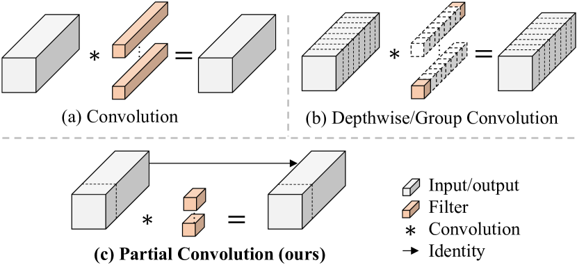
This paper aims to eliminate the discrepancy by developing a simple yet fast and effective operator that maintains high FLOPS with reduced FLOPs. Specifically, we reexamine existing operators, particularly DWConv, in terms of the computational speed – FLOPS. We uncover that the main reason causing the low FLOPS issue is frequent memory access. We then propose a novel partial convolution (PConv) as a competitive alternative that reduces the computational redundancy as well as the number of memory access. Fig. 1 illustrates the design of our PConv. It takes advantage of redundancy within the feature maps and systematically applies a regular convolution (Conv) on only a part of the input channels while leaving the remaining ones untouched. By nature, PConv has lower FLOPs than the regular Conv while having higher FLOPS than the DWConv/GConv. In other words, PConv better exploits the on-device computational capacity. PConv is also effective in extracting spatial features as empirically validated later in the paper.

We further introduce FasterNet, which is primarily built upon our PConv, as a new family of networks that run highly fast on various devices. In particular, our FasterNet achieves state-of-the-art performance for classification, detection, and segmentation tasks while having much lower latency and higher throughput. For example, our tiny FasterNet-T0 is $2.8\times$, $3.3\times$, and $2.4\times$ faster than MobileViT-XXS [48] on GPU, CPU, and ARM processors, respectively, while being 2.9% more accurate on ImageNet-1k. Our large FasterNet-L achieves 83.5% top-1 accuracy, on par with the emerging Swin-B [41], while offering 36% higher throughput on GPU and saving 37% compute time on CPU. To summarize, our contributions are as follows:

• We point out the importance of achieving higher FLOPS beyond simply reducing FLOPs for faster neural networks.

• We introduce a simple yet fast and effective operator called PConv, which has a high potential to replace the existing go-to choice, DWConv.

• We introduce FasterNet which runs favorably and universally fast on a variety of devices such as GPU, CPU, and ARM processors.

• We conduct extensive experiments on various tasks and validate the high speed and effectiveness of our PConv and FasterNet.

2 Related Work

We briefly review prior works on fast and efficient neural networks and differentiate this work from them.

CNN.  CNNs are the mainstream architecture in the computer vision field, especially when it comes to deployment in practice, where being fast is as important as being accurate. Though there have been numerous studies [55, 56, 7, 8, 83, 33, 21, 86] to achieve higher efficiency, the rationale behind them is more or less to perform a low-rank approximation. Specifically, the group convolution [31] and the depthwise separable convolution [55] (consisting of depthwise and pointwise convolutions) are probably the most popular ones. They have been widely adopted in mobile/edge-oriented networks, such as MobileNets [25, 54, 24], ShuffleNets [84, 46], GhostNet [17], EfficientNets [61, 62], TinyNet [18], Xception [8], CondenseNet [27, 78], TVConv [4], MnasNet[60], and FBNet [74]. While they exploit the redundancy in filters to reduce the number of parameters and FLOPs, they suffer from increased memory access when increasing the network width to compensate for the accuracy drop. By contrast, we consider the redundancy in feature maps and propose a partial convolution to reduce FLOPs and memory access simultaneously.

ViT, MLP, and variants.  There is a growing interest in studying ViT ever since Dosovitskiy et al. [12] expanded the application scope of transformers [69] from machine translation [69] or forecasting [73] to the computer vision field. Many follow-up works have attempted to improve ViT in terms of training setting [65, 66, 58] and model design [41, 40, 72, 15, 85]. One notable trend is to pursue a better accuracy-latency trade-off by reducing the complexity of the attention operator [1, 68, 29, 45, 63], incorporating convolution into ViTs [10, 6, 57], or doing both [3, 34, 52, 49]. Besides, other studies [64, 35, 5] propose to replace the attention with simple MLP-based operators. However, they often evolve to be CNN-like [39]. In this paper, we focus on analyzing the convolution operations, particularly DWConv, due to the following reasons: First, the advantage of attention over convolution is unclear or debatable [71, 42]. Second, the attention-based mechanism generally runs slower than its convolutional counterparts and thus becomes less favorable for the current industry [48, 26]. Finally, DWConv is still a popular choice in many hybrid models, so it is worth a careful examination.

3 Design of PConv and FasterNet

In this section, we first revisit DWConv and analyze the issue with its frequent memory access. We then introduce PConv as a competitive alternative operator to resolve the issue. After that, we introduce FasterNet and explain its details, including design considerations.

3.1 Preliminary

DWConv is a popular variant of Conv and has been widely adopted as a key building block for many neural networks. For an input $𝐈\in {ℝ}^{c\times h\times w}$, DWConv applies $c$ filters $𝐖\in {ℝ}^{k\times k}$ to compute the output $𝐎\in {ℝ}^{c\times h\times w}$. As shown in Fig. 1(b), each filter slides spatially on one input channel and contributes to one output channel. This depthwise computation makes DWConv have as low FLOPs as $h\times w\times k^2\times c$ compared to a regular Conv with $h\times w\times k^2\times c^2$. While effective in reducing FLOPs, a DWConv, which is typically followed by a pointwise convolution, or PWConv, cannot be simply used to replace a regular Conv as it would incur a severe accuracy drop. Thus, in practice the channel number $c$ (or the network width) of DWConv is increased to $c^{\prime }\left(c^{\prime }>c\right)$ to compensate the accuracy drop, e.g., the width is expanded by six times for the DWConv in the inverted residual blocks [54]. This, however, results in much higher memory access that can cause non-negligible delay and slow down the overall computation, especially for I/O-bound devices. In particular, the number of memory access now escalates to

$$h\times w\times 2c^{\prime }+k^2\times c^{\prime }\approx h\times w\times 2c^{\prime },$$ (2)

which is higher than that of a regular Conv, i.e.,

$$h\times w\times 2c+k^2\times c^2\approx h\times w\times 2c.$$ (3)

Note that the $h\times w\times 2c^{\prime }$ memory access is spent on the I/O operation, which is deemed to be already the minimum cost and hard to optimize further.

Figure 3: Visualization of feature maps in an intermediate layer of a pre-trained ResNet50, with the top-left image as the input. Qualitatively, we can see the high redundancies across different channels.

3.2 Partial convolution as a basic operator

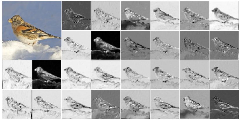
We below demonstrate that the cost can be further optimized by leveraging the feature maps’ redundancy. As visualized in Fig. 3, the feature maps share high similarities among different channels. This redundancy has also been covered in many other works [17, 82], but few of them make full use of it in a simple yet effective way.

Figure 4: Overall architecture of our FasterNet. It has four hierarchical stages, each with a stack of FasterNet blocks and preceded by an embedding or merging layer. The last three layers are used for feature classification. Within each FasterNet block, a PConv layer is followed by two PWConv layers. We put normalization and activation layers only after the middle layer to preserve the feature diversity and achieve lower latency.

Figure 5: Comparison of convolutional variants. A PConv followed by a PWConv (a) resembles a T-shaped Conv (b), which spends more computation on the center position compared to a regular Conv (c).

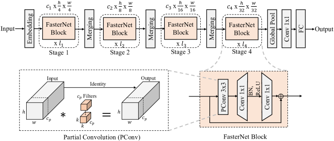
Specifically, we propose a simple PConv to reduce computational redundancy and memory access simultaneously. The bottom-left corner in Fig. 4 illustrates how our PConv works. It simply applies a regular Conv on only a part of the input channels for spatial feature extraction and leaves the remaining channels untouched. For contiguous or regular memory access, we consider the first or last consecutive $c_p$ channels as the representatives of the whole feature maps for computation. Without loss of generality, we consider the input and output feature maps to have the same number of channels. Therefore, the FLOPs of a PConv are only

$$h\times w\times k^2\times c_p^2.$$ (4)

With a typical partial ratio $r=\frac{c_p}{c}=\frac{1}{4}$, the FLOPs of a PConv is only $\frac{1}{16}$ of a regular Conv. Besides, PConv has a smaller amount of memory access, i.e.,

$$h\times w\times 2c_p+k^2\times c_p^2\approx h\times w\times 2c_p,$$ (5)

which is only $\frac{1}{4}$ of a regular Conv for $r=\frac{1}{4}$.

Since there are only $c_p$ channels utilized for spatial feature extraction, one may ask if we can simply remove the remaining $(c-c_p)$ channels? If so, PConv would degrade to a regular Conv with fewer channels, which deviates from our objective to reduce redundancy. Note that we keep the remaining channels untouched instead of removing them from the feature maps. It is because they are useful for a subsequent PWConv layer, which allows the feature information to flow through all channels.

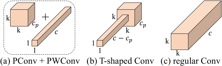
3.3 PConv followed by PWConv

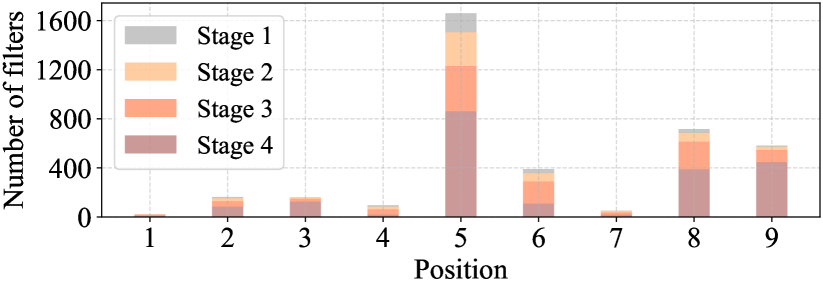
To fully and efficiently leverage the information from all channels, we further append a pointwise convolution (PWConv) to our PConv. Their effective receptive field together on the input feature maps looks like a T-shaped Conv, which focuses more on the center position compared to a regular Conv uniformly processing a patch, as shown in Fig. 5. To justify this T-shaped receptive field, we first evaluate the importance of each position by calculating the position-wise Frobenius norm. We assume that a position tends to be more important if it has a larger Frobenius norm than other positions. For a regular Conv filter $𝐅\in {ℝ}^{k^2\times c}$, the Frobenius norm at position $i$ is calculated by $\Vert {𝐅}_i\Vert =\sqrt{{\sum }_{j=1}^c{|f_{ij}|}^2},$ for $i=1,2,3\mathrm{\dots },k^2$. We consider a salient position to be the one with the maximum Frobenius norm. We then collectively examine each filter in a pre-trained ResNet18, find out their salient positions, and plot a histogram of the salient positions. Results in Fig. 6 show that the center position turns out to be the salient position most frequently among the filters. In other words, the center position weighs more than its surrounding neighbors. This is consistent with the T-shaped computation which concentrates on the center position.

While the T-shaped Conv can be directly used for efficient computation, we show that it is better to decompose the T-shaped Conv into a PConv and a PWConv because the decomposition exploits the inter-filter redundancy and further saves FLOPs. For the same input $𝐈\in {ℝ}^{c\times h\times w}$ and output $𝐎\in {ℝ}^{c\times h\times w}$, a T-shaped Conv’s FLOPs can be calculated as

$$h\times w\times \left(k^2\times c_p\times c+c\times \left(c-c_p\right)\right),$$ (6)

which is higher than the FLOPs of a PConv and a PWConv, i.e.,

$$h\times w\times (k^2\times c_p^2+c^2),$$ (7)

where $(k^2-1)c>k^2{c}_p,$ e.g. when $c_p=\frac{c}{4}$ and $k=3.$ Besides, we can readily leverage the regular Conv for the two-step implementation.

3.4 FasterNet as a general backbone

Given our novel PConv and off-the-shelf PWConv as the primary building operators, we further propose FasterNet, a new family of neural networks that runs favorably fast and is highly effective for many vision tasks. We aim to keep the architecture as simple as possible, without bells and whistles, to make it hardware-friendly in general.

We present the overall architecture in Fig. 4. It has four hierarchical stages, each of which is preceded by an embedding layer (a regular Conv $4\times 4$ with stride 4) or a merging layer (a regular Conv $2\times 2$ with stride 2) for spatial downsampling and channel number expanding. Each stage has a stack of FasterNet blocks. We observe that the blocks in the last two stages consume less memory access and tend to have higher FLOPS, as empirically validated in Tab. 1. Thus, we put more FasterNet blocks and correspondingly assign more computations to the last two stages. Each FasterNet block has a PConv layer followed by two PWConv (or Conv $1\times 1$) layers. Together, they appear as inverted residual blocks where the middle layer has an expanded number of channels, and a shortcut connection is placed to reuse the input features.

In addition to the above operators, the normalization and activation layers are also indispensable for high-performing neural networks. Many prior works [20, 54, 17], however, overuse such layers throughout the network, which may limit the feature diversity and thus hurt the performance. It can also slow down the overall computation. By contrast, we put them only after each middle PWConv to preserve the feature diversity and achieve lower latency. Besides, we use the batch normalization (BN) [30] instead of other alternative ones [2, 67, 75]. The benefit of BN is that it can be merged into its adjacent Conv layers for faster inference while being as effective as the others. As for the activation layers, we empirically choose GELU [22] for smaller FasterNet variants and ReLU [51] for bigger FasterNet variants, considering both running time and effectiveness. The last three layers, i.e. a global average pooling, a Conv $1\times 1$, and a fully-connected layer, are used together for feature transformation and classification.

To serve a wide range of applications under different computational budgets, we provide tiny, small, medium, and large variants of FasterNet, referred to as FasterNet-T0/1/2, FasterNet-S, FasterNet-M, and FasterNet-L, respectively. They share a similar architecture but vary in depth and width. Detailed architecture specifications are provided in the appendix.

Figure 6: Histogram of salient position distribution for the regular Conv $3\times 3$ filters in a pre-trained ResNet18. The histogram contains four kinds of bars, corresponding to different stages in the network. In all stages, the center position (position 5) appears as a salient position most frequently.

4 Experimental Results

We first examine the computational speed of our PConv and its effectiveness when combined with a PWConv. We then comprehensively evaluate the performance of our FasterNet for classification, detection, and segmentation tasks. Finally, we conduct a brief ablation study.

To benchmark the latency and throughput, we choose the following three typical processors, which cover a wide range of computational capacity: GPU (2080Ti), CPU (Intel i9-9900X, using a single thread), and ARM (Cortex-A72, using a single thread). We report their latency for inputs with a batch size of 1 and throughput for inputs with a batch size of 32. During inference, the BN layers are merged to their adjacent layers wherever applicable.

4.1 PConv is fast with high FLOPS

Operator	Feature map size	FLOPs (M), $\times$10 layers	GPU		CPU		ARM
			Throughput (fps)	FLOPS (G/s)	Latency (ms)	FLOPS (G/s)	Latency (ms)	FLOPS (G/s)
Conv 3$\times$3	96$\times$56$\times$56	2601	3010	7824	35.67	72.90	779.57	3.33
	192$\times$28$\times$28	2601	4893	12717	28.41	91.53	619.64	4.19
	384$\times$14$\times$14	2601	4558	11854	31.85	81.66	595.09	4.37
	768$\times$7$\times$7	2601	3159	8212	62.71	41.47	662.17	3.92
	Average		-	10151	-	71.89	-	3.95
GConv 3$\times$3 (16 groups)	96$\times$56$\times$56	162	2888	469	21.90	7.42	166.30	0.97
	192$\times$28$\times$28	162	10811	1754	7.58	21.44	96.22	1.68
	384$\times$14$\times$14	162	15534	2514	4.40	36.88	63.57	2.55
	768$\times$7$\times$7	162	16000	2598	4.28	37.97	65.20	2.49
	Average		-	1833	-	25.93	-	1.92
DWConv 3$\times$3	96$\times$56$\times$56	27.09	11940	323	3.59	7.52	108.70	0.24
	192$\times$28$\times$28	13.54	23358	315	1.97	6.86	82.01	0.16
	384$\times$14$\times$14	6.77	46377	313	1.06	6.35	94.89	0.07
	768$\times$7$\times$7	3.38	88889	302	0.68	4.93	150.89	0.02
	Average		-	313	-	6.42	-	0.12
PConv 3$\times$3 (ours, with $r=\frac{1}{4}$)	96$\times$56$\times$56	162	9215	1493	5.46	29.67	85.30	1.90
	192$\times$28$\times$28	162	14360	2326	3.09	52.43	66.46	2.44
	384$\times$14$\times$14	162	24408	3954	3.58	45.25	49.98	3.24
	768$\times$7$\times$7	162	32866	5324	5.02	32.27	48.30	3.35
	Average		-	3274	-	39.91	-	2.73

Table 1: On-device FLOPS for different operations. PConv appears as an appealing choice for high FLOPS with reduced FLOPs.

We below show that our PConv is fast and better exploits the on-device computational capacity. Specifically, we stack 10 layers of pure PConv and take feature maps of typical dimensions as inputs. We then measure FLOPs and latency/throughput on GPU, CPU, and ARM processors, which also allow us to further compute FLOPS. We repeat the same procedure for other convolutional variants and make comparisons.

Results in Tab. 1 show that PConv is overall an appealing choice for high FLOPS with reduced FLOPs. It has only $\frac{1}{16}$ FLOPs of a regular Conv and achieves $10.5\times$, $6.2\times$, and $22.8\times$ higher FLOPS than the DWConv on GPU, CPU, and ARM, respectively. We are unsurprised to see that the regular Conv has the highest FLOPS as it has been constantly optimized for years. However, its total FLOPs and latency/throughput are unaffordable. GConv and DWConv, despite their significant reduction in FLOPs, suffer from a drastic decrease in FLOPS. In addition, they tend to increase the number of channels to compensate for the performance drop, which, however, increase their latency.

4.2 PConv is effective together with PWConv

We next show that a PConv followed by a PWConv is effective in approximating a regular Conv to transform the feature maps. To this end, we first build four datasets by feeding the ImageNet-1k val split images into a pre-trained ResNet50, and extract the feature maps before and after the first Conv $3\times 3$ in each of the four stages. Each feature map dataset is further spilt into the train (70%), val (10%), and test (20%) subsets. We then build a simple network consisting of a PConv followed by a PWConv and train it on the feature map datasets with a mean squared error loss. For comparison, we also build and train networks for DWConv + PWConv and GConv + PWConv under the same setting.

Tab. 2 shows that PConv + PWConv achieve the lowest test loss, meaning that they better approximate a regular Conv in feature transformation. The results also suggest that it is sufficient and efficient to capture spatial features from only a part of the feature maps. PConv shows a great potential to be the new go-to choice in designing fast and effective neural networks.

Stage	DWConv+PWConv	GConv+PWConv (16 groups)	PConv+PWConv $r=\frac{1}{4}$
1	0.0089	0.0065	0.0069
2	0.0158	0.0137	0.0136
3	0.0214	0.0202	0.0172
4	0.0130	0.0128	0.0115
Average	0.0148	0.0133	0.0123

Table 2: A PConv followed by a PWConv well approximates the regular Conv $3\times 3$ at different stages of a pre-trained ResNet50. PConv + PWConv together have the lowest test loss on average.

4.3 FasterNet on ImageNet-1k classification

Figure 7: FasterNet has the highest efficiency in balancing accuracy-throughput and accuracy-latency trade-offs for different devices. To save space and make the plots more proportionate, we showcase network variants within a certain range of latency. Full plots can be found in the appendix, which show consistent results.

Network	Params (M)	FLOPs (G)	Throughput on GPU (fps) $\uparrow$	Latency on CPU (ms) $\downarrow$	Latency on ARM (ms) $\downarrow$	Acc. (%)
ShuffleNetV2 $\times$1.5 [46]	3.5	0.30	4878	12.1	266	72.6
MobileNetV2 [54]	3.5	0.31	4198	12.2	442	72.0
MobileViT-XXS [48]	1.3	0.42	2393	30.8	348	69.0
EdgeNeXt-XXS [47]	1.3	0.26	2765	15.7	239	71.2
FasterNet-T0	3.9	0.34	6807	9.2	143	71.9
GhostNet $\times$1.3 [17]	7.4	0.24	2988	17.9	481	75.7
ShuffleNetV2 $\times$2 [46]	7.4	0.59	3339	17.8	403	74.9
MobileNetV2 $\times$1.4 [54]	6.1	0.60	2711	22.6	650	74.7
MobileViT-XS [48]	2.3	1.05	1392	40.8	648	74.8
EdgeNeXt-XS [47]	2.3	0.54	1738	24.4	434	75.0
PVT-Tiny [72]	13.2	1.94	1266	55.6	708	75.1
FasterNet-T1	7.6	0.85	3782	17.7	285	76.2
CycleMLP-B1 [5]	15.2	2.10	865	116.1	892	79.1
PoolFormer-S12 [79]	11.9	1.82	1439	49.0	665	77.2
MobileViT-S [48]	5.6	2.03	1039	56.7	941	78.4
EdgeNeXt-S [47]	5.6	1.26	1128	39.2	743	79.4
ResNet50 [20, 42]	25.6	4.11	959	73.0	1131	78.8
FasterNet-T2	15.0	1.91	1991	33.5	497	78.9
CycleMLP-B2 [5]	26.8	3.90	528	186.3	1502	81.6
PoolFormer-S24 [79]	21.4	3.41	748	92.8	1261	80.3
PoolFormer-S36 [79]	30.9	5.00	507	138.0	1860	81.4
ConvNeXt-T [42]	28.6	4.47	657	86.3	1889	82.1
Swin-T [41]	28.3	4.51	609	122.2	1424	81.3
PVT-Small [72]	24.5	3.83	689	89.6	1345	79.8
PVT-Medium [72]	44.2	6.69	438	143.6	2142	81.2
FasterNet-S	31.1	4.56	1029	71.2	1103	81.3
PoolFormer-M36 [79]	56.2	8.80	320	215.0	2979	82.1
ConvNeXt-S [42]	50.2	8.71	377	153.2	3484	83.1
Swin-S [41]	49.6	8.77	348	224.2	2613	83.0
PVT-Large [72]	61.4	9.85	306	203.4	3101	81.7
FasterNet-M	53.5	8.74	500	129.5	2092	83.0
PoolFormer-M48 [79]	73.5	11.59	242	281.8	OOM	82.5
ConvNeXt-B [42]	88.6	15.38	253	257.1	OOM	83.8
Swin-B [41]	87.8	15.47	237	349.2	OOM	83.5
FasterNet-L	93.5	15.52	323	219.5	OOM	83.5

Table 3: Comparison on ImageNet-1k benchmark. Models with similar top-1 accuracy are grouped together. For each group, our FasterNet achieves the highest throughput on GPU and the lowest latency on CPU and ARM. All models are evaluated at $224\times 224$ resolution except for the MobileViT and EdgeNeXt with $256\times 256$. OOM is short for out of memory.

Backbone	Params (M)	FLOPs (G)	Latency on GPU (ms)	$A{P}^b$	$A{P}_{50}^b$	$A{P}_{75}^b$	$A{P}^m$	$A{P}_{50}^m$	$A{P}_{75}^m$
ResNet50 [20]	44.2	253	54.9	38.0	58.6	41.4	34.4	55.1	36.7
PoolFormer-S24 [79]	41.0	233	111.0	40.1	62.2	43.4	37.0	59.1	39.6
PVT-Small [72]	44.1	238	89.5	40.4	62.9	43.8	37.8	60.1	40.3
FasterNet-S	49.0	258	54.3	39.9	61.2	43.6	36.9	58.1	39.7
ResNet101 [20]	63.2	329	68.9	40.4	61.1	44.2	36.4	57.7	38.8
ResNeXt101-32$\times$4d [77]	62.8	333	80.5	41.9	62.5	45.9	37.5	59.4	40.2
PoolFormer-S36 [79]	50.5	266	146.9	41.0	63.1	44.8	37.7	60.1	40.0
PVT-Medium [72]	63.9	295	117.3	42.0	64.4	45.6	39.0	61.6	42.1
FasterNet-M	71.2	344	71.4	43.0	64.4	47.4	39.1	61.5	42.3
ResNeXt101-64$\times$4d [77]	101.9	487	112.9	42.8	63.8	47.3	38.4	60.6	41.3
PVT-Large [72]	81.0	358	152.2	42.9	65.0	46.6	39.5	61.9	42.5
FasterNet-L	110.9	484	93.8	44.0	65.6	48.2	39.9	62.3	43.0

Table 4: Results on COCO object detection and instance segmentation benchmarks. FLOPs are calculated with image size (1280, 800).

Ablation	Variant	Throughput on GPU (fps)	Latency on CPU (ms)	Latency on ARM (ms)	Acc. (%)
Partial ratio	${\text{T0}}^{\ast }$ w/ $r=1/2$	6626	9.6	145	71.7
	T0 w/ $r=1/4$	6807	9.2	143	71.9
	${\text{T0}}^{\ast }$ w/ $r=1/8$	6204	8.9	140	71.3
Normalization	T0 w/ BN	6807	9.2	143	71.9
	T0 w/ LN	5515	10.7	159	71.9
Activation	T0 w/ ReLU	6929	8.2	114	71.3
	${\text{T0}}^{\ast }$ w/ ReLU	5866	9.3	143	71.7
	T0 w/ GELU	6807	9.2	143	71.9
	T2 w/ ReLU	1991	33.5	497	78.9
	T2 w/ GELU	1985	35.4	557	78.7

Table 5: Ablation on the partial ratio, normalization, and activation of FasterNet. Rows highlighted in grey are the default settings. ${\text{T0}}^{\ast }$ denotes T0 variants with modified network width and depth.

To verify the effectiveness and efficiency of our FasterNet, we first conduct experiments on the large-scale ImageNet-1k classification dataset [53]. It covers 1k categories of common objects and contains about 1.3M labeled images for training and 50k labeled images for validation. We train our models for 300 epochs using AdamW optimizer [44]. We set the batch size to 2048 for the FasterNet-M/L and 4096 for other variants. We use cosine learning rate scheduler [43] with a peak value of $0.001\cdot \text{batch size}/1024$ and a 20-epoch linear warmup. We apply commonly-used regularization and augmentation techniques, including Weight Decay [32], Stochastic Depth [28], Label Smoothing [59], Mixup [81], Cutmix [80] and Rand Augment [9], with varying magnitudes for different FasterNet variants. To reduce the training time, we use $192\times 192$ resolution for the first 280 training epochs and $224\times 224$ for the remaining 20 epochs. For fair comparison, we do not use knowledge distillation [23] and neural architecture search [87]. We report our top-1 accuracy on the validation set with a center crop at $224\times 224$ resolution and a 0.9 crop ratio. Detailed training and validation settings are provided in the appendix.

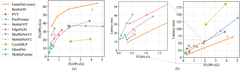
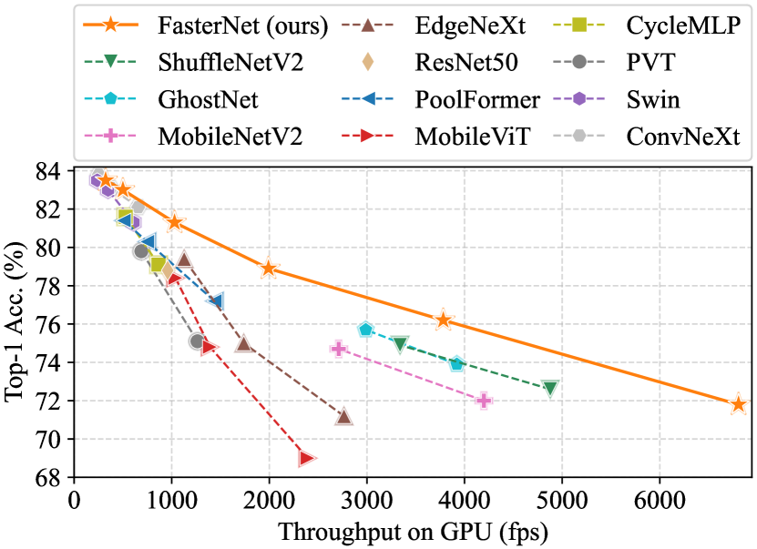
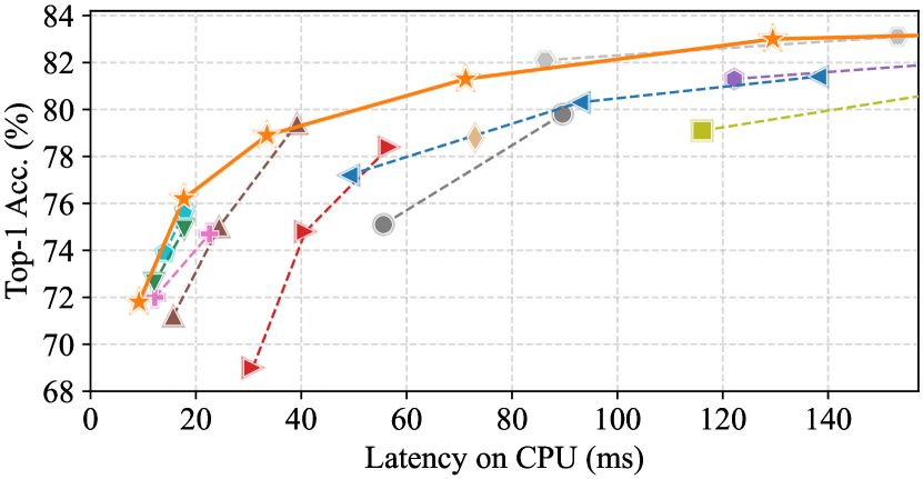
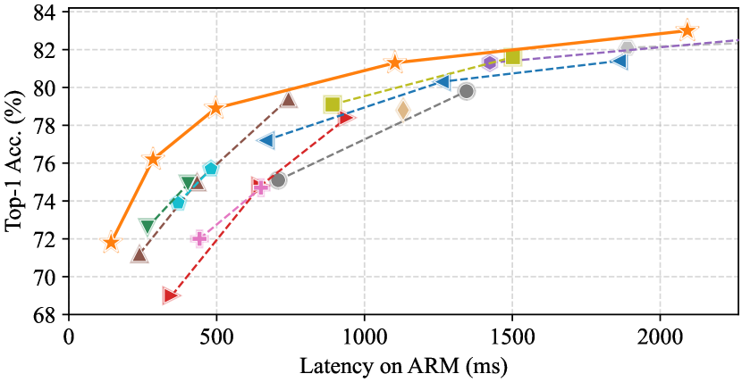
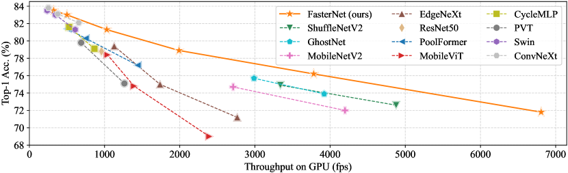
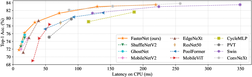
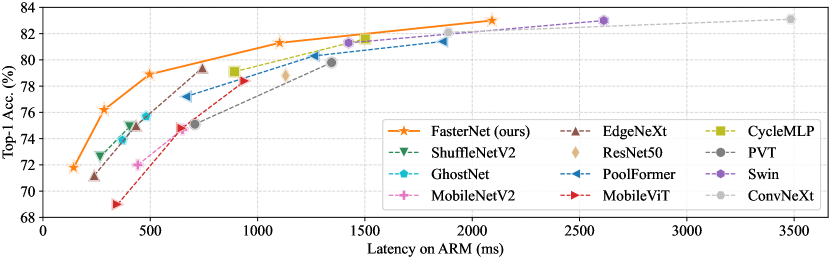
Fig. 7 and Tab. 3 demonstrate the superiority of our FasterNet over state-of-the-art classification models. The trade-off curves in Fig. 7 clearly show that FasterNet sets the new state-of-the-art in balancing accuracy and latency/throughput among all the networks examined. From another perspective, FasterNet runs faster than various CNN, ViT and MLP models on a wide range of devices, when having similar top-1 accuracy. As quantitatively shown in Tab. 3, FasterNet-T0 is $2.8\times$, $3.3\times$, and $2.4\times$ faster than MobileViT-XXS [48] on GPU, CPU, and ARM processors, respectively, while being 2.9% more accurate. Our large FasterNet-L achieves 83.5% top-1 accuracy, comparable to the emerging Swin-B [41] and ConvNeXt-B [42] while having 36% and 28% higher inference throughput on GPU, as well as saving 37% and 15% compute time on CPU. Given such promising results, we highlight that our FasterNet is much simpler than many other models in terms of architectural design, which showcases the feasibility of designing simple yet powerful neural networks.

4.4 FasterNet on downstream tasks

To further evaluate the generalization ability of FasterNet, we conduct experiments on the challenging COCO dataset [36] for object detection and instance segmentation. As a common practice, we employ the ImageNet pre-trained FasterNet as a backbone and equip it with the popular Mask R-CNN detector [19]. To highlight the effectiveness of the backbone itself, we simply follow PoolFormer [79] and adopt an AdamW optimizer, a $1\times$ training schedule (12 epochs), a batch size of 16, and other training settings without further hyper-parameter tuning.

Tab. 4 shows the results for comparison between FasterNet and representative models. FasterNet consistently outperforms ResNet and ResNext by having higher average precision (AP) with similar latency. Specifically, FasterNet-S yields $+1.9$ higher box AP and $+2.4$ higher mask AP compared to the standard baseline ResNet50. FasterNet is also competitive against the ViT variants. Under similar FLOPs, FasterNet-L reduces PVT-Large’s latency by 38%, i.e., from 152.2 ms to 93.8 ms on GPU, and achieves $+1.1$ higher box AP and $+0.4$ higher mask AP.

4.5 Ablation study

We conduct a brief ablation study on the value of partial ratio $r$ and the choices of activation and normalization layers. We compare different variants in terms of ImageNet top-1 accuracy and on-device latency/throughput. Results are summarized in Tab. 5. For the partial ratio $r$, we set it to $\frac{1}{4}$ for all FasterNet variants by default, which achieves higher accuracy, higher throughput, and lower latency at similar complexity. A too large partial ratio $r$ would make PConv degrade to a regular Conv, while a too small value would render PConv less effective in capturing the spatial features. For the normalization layers, we choose BatchNorm over LayerNorm because BatchNorm can be merged into its adjacent convolutional layers for faster inference while it is as effective as LayerNorm in our experiment. For the activation function, interestingly, we empirically found that GELU fits FasterNet-T0/T1 models more efficiently than ReLU. It, however, becomes opposite for FasterNet-T2/S/M/L. Here we only show two examples in Tab. 5 due to space constraint. We conjecture that GELU strengthens FasterNet-T0/T1 by having higher non-linearity, while the benefit fades away for larger FasterNet variants.

5 Conclusion

In this paper, we have investigated the common and unresolved issue that many established neural networks suffer from low floating-point operations per second (FLOPS). We have revisited a bottleneck operator, DWConv, and analyzed its main cause for a slowdown – frequent memory access. To overcome the issue and achieve faster neural networks, we have proposed a simple yet fast and effective operator, PConv, that can be readily plugged into many existing networks. We have further introduced our general-purpose FasterNet, built upon our PConv, that achieves state-of-the-art speed and accuracy trade-off on various devices and vision tasks. We hope that our PConv and FasterNet would inspire more research on simple yet effective neural networks, going beyond academia to impact the industry and community directly.

Acknowledgement  This work was supported, in part, by Hong Kong General Research Fund under grant number 16200120. The work of C.-H. Lee was supported, in part, by the NSF under Grant IIS-2209921.

Appendix

In this appendix, we provide further details on the experimental settings, full comparison plots, architectural configurations, PConv implementations, comparisons with related work, limitations, and future work.

Appendix A ImageNet-1k experimental settings

We provide ImageNet-1k training and evaluation settings in Tab. 6. They can be used for reproducing our main results in Tab. 3 and Fig. 7. Different FasterNet variants vary in the magnitude of regularization and augmentation techniques. The magnitude increases as the model becomes larger to alleviate overfitting and improve accuracy. Note that most of the compared works in Tab. 3 and Fig. 7, e.g., MobileViT, EdgeNext, PVT, CycleMLP, ConvNeXt, Swin, etc., also adopt such advanced training techniques (ADT). Some even heavily rely on the hyper-parameter search. For others w/o ADT, i.e., ShuffleNetV2, MobileNetV2, and GhostNet, though the comparison is not totally fair, we include them for reference.

Appendix B Downstream tasks experimental settings

For object detection and instance segmentation on the COCO2017 dataset, we equip our FasterNet backbone with the popular Mask R-CNN detector. We use ImageNet-1k pre-trained weights to initialize the backbone and Xavier to initialize the add-on layers. Detailed settings are summarized in Tab. 7.

Appendix C Full comparison plots on ImageNet-1k

Fig. 8 shows the full comparison plots on ImageNet-1k, which is the extension of Fig. 7 in the main paper with a larger range of latency. Fig. 8 shows consistent results that FasterNet strikes better trade-offs than others in balancing accuracy and latency/throughput on GPU, CPU, and ARM processors.

Appendix D Detailed architectural configurations

We present the detailed architectural configurations in Tab. 8. While different FasterNet variants share a unified architecture, they vary in the network width (the number of channels) and network depth (the number of FasterNet blocks at each stage). The classifier at the end of the architecture is used for classification tasks but removed for other downstream tasks.

Variants	T0	T1	T2	S	M	L
Train Res	192 for epoch 1$\sim$280, 224 for epoch 281$\sim$300
Test Res	224
Epochs	300
# of forward pass	188k
Batch size	4096	4096	4096	4096	2048	2048
Optimizer	AdamW
Momentum	0.9/0.999
LR	0.004	0.004	0.004	0.004	0.002	0.002
LR decay	cosine
Weight decay	0.005	0.01	0.02	0.03	0.05	0.05
Warmup epochs	20
Warmup schedule	linear
Label smoothing	0.1
Dropout	✗
Stoch. Depth	✗	0.02	0.05	0.1	0.2	0.3
Repeated Aug	✗
Gradient Clip.	✗	✗	✗	✗	1	0.01
H. flip	✓
RRC	✓
Rand Augment	✗	3/0.5	5/0.5	7/0.5	7/0.5	7/0.5
Auto Augment	✗
Mixup alpha	0.05	0.1	0.1	0.3	0.5	0.7
Cutmix alpha	1.0
Erasing prob.	✗
Color Jitter	✗
PCA lighting	✗
SWA	✗
EMA	✗
Layer scale	✗
CE loss	✓
BCE loss	✗
Mixed precision	✓
Test crop ratio	0.9
Top-1 acc. (%)	71.9	76.2	78.9	81.3	83.0	83.5

Table 6: ImageNet-1k training and evaluation settings for different FasterNet variants.

Variants	S	M	L
Train and test Res	shorter side $=$ 800, longer side $\le$ 1333
Batch size	16 (2 on each GPU)
Optimizer	AdamW
Train schedule	1$\times$ schedule (12 epochs)
Weight decay	0.0001
Warmup schedule	linear
Warmup iterations	500
LR decay	StepLR at epoch 8 and 11 with decay rate 0.1
LR	0.0002	0.0001	0.0001
Stoch. Depth	0.15	0.2	0.3

Table 7: Experimental settings of object detection and instance segmentation on the COCO2017 dataset.

Figure 8: Comparison of FasterNet with state-of-the-art networks. FasterNet consistently achieves better accuracy-throughput (the top plot) and accuracy-latency (the medium and bottom plots) trade-offs than others.

Appendix E More comparisons with related work

Improving FLOPS.  There are a few other works [11, 76] also looking into the FLOPS issue and trying to improve it. They generally follow existing operators and try to find their proper configurations, e.g., RepLKNet [11] simply increases the kernel size while TRT-ViT [76] reorders different blocks in the architecture. By contrast, this paper advances the field by proposing a novel and efficient PConv, opening up new directions and potentially larger room for FLOPS improvement.

Name	Output size	Layer specification		T0	T1	T2	S	M	L
Embedding	$\frac{h}{4}\times \frac{w}{4}$	Conv_4_$c$_4, BN	# Channels $c$	40	64	96	128	144	192
Stage 1	$\frac{h}{4}\times \frac{w}{4}$	$\left[\begin{array}{c}\text{PConv\_3\_}c\text{\_1\_1/4,}\\ \text{Conv\_1\_}2c\text{\_1,}\\ \text{BN, Acti,}\\ \text{Conv\_1\_}c\text{\_1}\end{array}\right]\times b_1$	# Blocks $b_1$	1	1	1	1	3	3
Merging	$\frac{h}{8}\times \frac{w}{8}$	Conv_2_$2c$_2, BN	# Channels $2c$	80	128	192	256	288	384
Stage 2	$\frac{h}{8}\times \frac{w}{8}$	$\left[\begin{array}{c}\text{PConv\_3\_}2c\text{\_1\_1/4,}\\ \text{Conv\_1\_}4c\text{\_1,}\\ \text{BN, Acti,}\\ \text{Conv\_1\_}2c\text{\_1}\end{array}\right]\times b_2$	# Blocks $b_2$	2	2	2	2	4	4
Merging	$\frac{h}{16}\times \frac{w}{16}$	Conv_2_$4c$_2, BN	# Channels $4c$	160	256	384	512	576	768
Stage 3	$\frac{h}{16}\times \frac{w}{16}$	$\left[\begin{array}{c}\text{PConv\_3\_}4c\text{\_1\_1/4,}\\ \text{Conv\_1\_}8c\text{\_1,}\\ \text{BN, Acti,}\\ \text{Conv\_1\_}4c\text{\_1}\end{array}\right]\times b_3$	# Blocks $b_3$	8	8	8	13	18	18
Merging	$\frac{h}{32}\times \frac{w}{32}$	Conv_2_$8c$_2, BN	# Channels $8c$	320	512	768	1024	1152	1536
Stage 4	$\frac{h}{32}\times \frac{w}{32}$	$\left[\begin{array}{c}\text{PConv\_3\_}8c\text{\_1\_1/4,}\\ \text{Conv\_1\_}16c\text{\_1,}\\ \text{BN, Acti,}\\ \text{Conv\_1\_}8c\text{\_1}\end{array}\right]\times b_4$	# Blocks $b_4$	2	2	2	2	3	3
Classifier	$1\times 1$	Global average pool, Conv_1_1280_1, Acti, FC_1000	Acti	GELU	GELU	ReLU	ReLU	ReLU	ReLU
FLOPs (G)				0.34	0.85	1.90	4.55	8.72	15.49
Params (M)				3.9	7.6	15.0	31.1	53.5	93.4

Table 8: Configurations of different FasterNet variants. “Conv_$k$_$c$_$s$” means a convolutional layer with the kernel size of $k$, the output channels of $c$, and the stride of $s$. “PConv$\mathrm{\_}k\mathrm{\_}c\mathrm{\_}s\mathrm{\_}r$” means a partial convolution with an extra parameter, the partial ratio of $r$. “FC_1000” means a fully connected layer with 1000 output channels. $h\times w$ is the input size while $b_i$ is the number of FasterNet blocks at stage $i$. The FLOPs are calculated given the input size of $224\times 224$.

PConv vs. GConv.  PConv is schematically equivalent to a modified GConv [31] that operates on a single group and leaves other groups untouched. Though simple, such a modification remains unexplored before. It’s also significant in the sense that it prevents the operator from excessive memory access and is computationally more efficient. From the perspective of low-rank approximations, PConv improves GConv by further reducing the intra-filter redundancy beyond the inter-filter redundancy [16].

FasterNet vs. ConvNeXt.  Our FasterNet appears similar to ConvNeXt [42] after substituting DWConv with our PConv. However, they are different in motivations. While ConvNeXt searches for a better structure by trial and error, we append PWConv after PConv to better aggregate information from all channels. Moreover, ConvNeXt follows ViT to use fewer activation functions, while we intentionally remove them from the middle of PConv and PWConv, to minimize their error in approximating a regular Conv.

Other paradigms for efficient inference.  Our work focuses on efficient network design, orthogonal to the other paradigms, e.g., neural architecture search (NAS) [13], network pruning [50], and knowledge distillation [23]. They can be applied in this paper for better performance. However, we opt not to do so to keep our core idea centered and to make the performance gain clear and fair.

Other partial/masked convolution works.  There are several works [38, 14, 37] sharing similar names with our PConv. However, they differ a lot in objectives and methods. For example, they apply filters on partial pixels to exclude invalid patches [38], enable self-supervised learning [14], or synthesize novel images [37], while we target at the channel dimension for efficient inference.

Appendix F Limitations and future work

We have demonstrated that PConv and FasterNet are fast and effective, being competitive with existing operators and networks. Yet there are some minor technical limitations of this paper. For one thing, PConv is designed to apply a regular convolution on only a part of the input channels while leaving the remaining ones untouched. Thus, the stride of the partial convolution should always be 1, in order to align the spatial resolution of the convolutional output and that of the untouched channels. Note that it is still feasible to down-sample the spatial resolution as there can be additional downsampling layers in the architecture. And for another, our FasterNet is simply built upon convolutional operators with a possibly limited receptive field. Future efforts can be made to enlarge its receptive field and combine it with other operators to pursue higher accuracy.

References

- [1] Alaaeldin Ali, Hugo Touvron, Mathilde Caron, Piotr Bojanowski, Matthijs Douze, Armand Joulin, Ivan Laptev, Natalia Neverova, Gabriel Synnaeve, Jakob Verbeek, et al. Xcit: Cross-covariance image transformers. Advances in neural information processing systems, 34:20014–20027, 2021.
- [2] Jimmy Lei Ba, Jamie Ryan Kiros, and Geoffrey E Hinton. Layer normalization. arXiv preprint arXiv:1607.06450, 2016.
- [3] Han Cai, Chuang Gan, and Song Han. Efficientvit: Enhanced linear attention for high-resolution low-computation visual recognition. arXiv preprint arXiv:2205.14756, 2022.
- [4] Jierun Chen, Tianlang He, Weipeng Zhuo, Li Ma, Sangtae Ha, and S-H Gary Chan. Tvconv: Efficient translation variant convolution for layout-aware visual processing. In Proceedings of the IEEE/CVF Conference on Computer Vision and Pattern Recognition, pages 12548–12558, 2022.
- [5] Shoufa Chen, Enze Xie, Chongjian Ge, Ding Liang, and Ping Luo. Cyclemlp: A mlp-like architecture for dense prediction. arXiv preprint arXiv:2107.10224, 2021.
- [6] Yinpeng Chen, Xiyang Dai, Dongdong Chen, Mengchen Liu, Xiaoyi Dong, Lu Yuan, and Zicheng Liu. Mobile-former: Bridging mobilenet and transformer. In Proceedings of the IEEE/CVF Conference on Computer Vision and Pattern Recognition, pages 5270–5279, 2022.
- [7] Yunpeng Chen, Haoqi Fan, Bing Xu, Zhicheng Yan, Yannis Kalantidis, Marcus Rohrbach, Shuicheng Yan, and Jiashi Feng. Drop an octave: Reducing spatial redundancy in convolutional neural networks with octave convolution. In Proceedings of the IEEE/CVF International Conference on Computer Vision, pages 3435–3444, 2019.
- [8] François Chollet. Xception: Deep learning with depthwise separable convolutions. In Proceedings of the IEEE conference on computer vision and pattern recognition, pages 1251–1258, 2017.
- [9] Ekin D Cubuk, Barret Zoph, Jonathon Shlens, and Quoc V Le. Randaugment: Practical automated data augmentation with a reduced search space. In Proceedings of the IEEE/CVF conference on computer vision and pattern recognition workshops, pages 702–703, 2020.
- [10] Zihang Dai, Hanxiao Liu, Quoc V Le, and Mingxing Tan. Coatnet: Marrying convolution and attention for all data sizes. Advances in Neural Information Processing Systems, 34:3965–3977, 2021.
- [11] Xiaohan Ding et al. Scaling up your kernels to 31x31: Revisiting large kernel design in cnns. In CVPR, 2022.
- [12] Alexey Dosovitskiy, Lucas Beyer, Alexander Kolesnikov, Dirk Weissenborn, Xiaohua Zhai, Thomas Unterthiner, Mostafa Dehghani, Matthias Minderer, Georg Heigold, Sylvain Gelly, et al. An image is worth 16x16 words: Transformers for image recognition at scale. arXiv preprint arXiv:2010.11929, 2020.
- [13] Thomas Elsken, Jan Hendrik Metzen, and Frank Hutter. Neural architecture search: A survey. The Journal of Machine Learning Research, 20(1):1997–2017, 2019.
- [14] Peng Gao, Teli Ma, Hongsheng Li, Jifeng Dai, and Yu Qiao. Convmae: Masked convolution meets masked autoencoders. arXiv preprint arXiv:2205.03892, 2022.
- [15] Benjamin Graham, Alaaeldin El-Nouby, Hugo Touvron, Pierre Stock, Armand Joulin, Hervé Jégou, and Matthijs Douze. Levit: a vision transformer in convnet’s clothing for faster inference. In Proceedings of the IEEE/CVF international conference on computer vision, pages 12259–12269, 2021.
- [16] Daniel Haase et al. Rethinking depthwise separable convolutions: How intra-kernel correlations lead to improved mobilenets. In CVPR, 2020.
- [17] Kai Han, Yunhe Wang, Qi Tian, Jianyuan Guo, Chunjing Xu, and Chang Xu. Ghostnet: More features from cheap operations. In Proceedings of the IEEE/CVF conference on computer vision and pattern recognition, pages 1580–1589, 2020.
- [18] Kai Han, Yunhe Wang, Qiulin Zhang, Wei Zhang, Chunjing Xu, and Tong Zhang. Model rubik’s cube: Twisting resolution, depth and width for tinynets. Advances in Neural Information Processing Systems, 33:19353–19364, 2020.
- [19] Kaiming He, Georgia Gkioxari, Piotr Dollár, and Ross Girshick. Mask r-cnn. In Proceedings of the IEEE international conference on computer vision, pages 2961–2969, 2017.
- [20] Kaiming He, Xiangyu Zhang, Shaoqing Ren, and Jian Sun. Deep residual learning for image recognition. In Proceedings of the IEEE conference on computer vision and pattern recognition, pages 770–778, 2016.
- [21] Tianlang He, Jiajie Tan, Weipeng Zhuo, Maximilian Printz, and S-H Gary Chan. Tackling multipath and biased training data for imu-assisted ble proximity detection. In IEEE INFOCOM 2022-IEEE Conference on Computer Communications, pages 1259–1268. IEEE, 2022.
- [22] Dan Hendrycks and Kevin Gimpel. Gaussian error linear units (gelus). arXiv preprint arXiv:1606.08415, 2016.
- [23] Geoffrey Hinton, Oriol Vinyals, Jeff Dean, et al. Distilling the knowledge in a neural network. arXiv preprint arXiv:1503.02531, 2(7), 2015.
- [24] Andrew Howard, Mark Sandler, Grace Chu, Liang-Chieh Chen, Bo Chen, Mingxing Tan, Weijun Wang, Yukun Zhu, Ruoming Pang, Vijay Vasudevan, et al. Searching for mobilenetv3. In Proceedings of the IEEE/CVF international conference on computer vision, pages 1314–1324, 2019.
- [25] Andrew G Howard, Menglong Zhu, Bo Chen, Dmitry Kalenichenko, Weijun Wang, Tobias Weyand, Marco Andreetto, and Hartwig Adam. Mobilenets: Efficient convolutional neural networks for mobile vision applications. arXiv preprint arXiv:1704.04861, 2017.
- [26] Han Hu, Zheng Zhang, Zhenda Xie, and Stephen Lin. Local relation networks for image recognition. In Proceedings of the IEEE/CVF International Conference on Computer Vision, pages 3464–3473, 2019.
- [27] Gao Huang, Shichen Liu, Laurens Van der Maaten, and Kilian Q Weinberger. Condensenet: An efficient densenet using learned group convolutions. In Proceedings of the IEEE conference on computer vision and pattern recognition, pages 2752–2761, 2018.
- [28] Gao Huang, Yu Sun, Zhuang Liu, Daniel Sedra, and Kilian Q Weinberger. Deep networks with stochastic depth. In European conference on computer vision, pages 646–661. Springer, 2016.
- [29] Tao Huang, Lang Huang, Shan You, Fei Wang, Chen Qian, and Chang Xu. Lightvit: Towards light-weight convolution-free vision transformers. arXiv preprint arXiv:2207.05557, 2022.
- [30] Sergey Ioffe and Christian Szegedy. Batch normalization: Accelerating deep network training by reducing internal covariate shift. In International conference on machine learning, pages 448–456. PMLR, 2015.
- [31] Alex Krizhevsky, Ilya Sutskever, and Geoffrey E Hinton. Imagenet classification with deep convolutional neural networks. Advances in neural information processing systems, 25, 2012.
- [32] Anders Krogh and John Hertz. A simple weight decay can improve generalization. Advances in neural information processing systems, 4, 1991.
- [33] Yunsheng Li, Yinpeng Chen, Xiyang Dai, Dongdong Chen, Mengchen Liu, Lu Yuan, Zicheng Liu, Lei Zhang, and Nuno Vasconcelos. Micronet: Improving image recognition with extremely low flops. In Proceedings of the IEEE/CVF International Conference on Computer Vision, pages 468–477, 2021.
- [34] Yanyu Li, Geng Yuan, Yang Wen, Eric Hu, Georgios Evangelidis, Sergey Tulyakov, Yanzhi Wang, and Jian Ren. Efficientformer: Vision transformers at mobilenet speed. arXiv preprint arXiv:2206.01191, 2022.
- [35] Dongze Lian, Zehao Yu, Xing Sun, and Shenghua Gao. As-mlp: An axial shifted mlp architecture for vision. arXiv preprint arXiv:2107.08391, 2021.
- [36] Tsung-Yi Lin, Michael Maire, Serge Belongie, James Hays, Pietro Perona, Deva Ramanan, Piotr Dollár, and C Lawrence Zitnick. Microsoft coco: Common objects in context. In European conference on computer vision, pages 740–755. Springer, 2014.
- [37] Guilin Liu, Aysegul Dundar, Kevin J Shih, Ting-Chun Wang, Fitsum A Reda, Karan Sapra, Zhiding Yu, Xiaodong Yang, Andrew Tao, and Bryan Catanzaro. Partial convolution for padding, inpainting, and image synthesis. IEEE Transactions on Pattern Analysis and Machine Intelligence, 2022.
- [38] Guilin Liu, Fitsum A Reda, Kevin J Shih, Ting-Chun Wang, Andrew Tao, and Bryan Catanzaro. Image inpainting for irregular holes using partial convolutions. In Proceedings of the European conference on computer vision (ECCV), pages 85–100, 2018.
- [39] Ruiyang Liu, Yinghui Li, Linmi Tao, Dun Liang, and Hai-Tao Zheng. Are we ready for a new paradigm shift? a survey on visual deep mlp. Patterns, 3(7):100520, 2022.
- [40] Ze Liu, Han Hu, Yutong Lin, Zhuliang Yao, Zhenda Xie, Yixuan Wei, Jia Ning, Yue Cao, Zheng Zhang, Li Dong, et al. Swin transformer v2: Scaling up capacity and resolution. In Proceedings of the IEEE/CVF Conference on Computer Vision and Pattern Recognition, pages 12009–12019, 2022.
- [41] Ze Liu, Yutong Lin, Yue Cao, Han Hu, Yixuan Wei, Zheng Zhang, Stephen Lin, and Baining Guo. Swin transformer: Hierarchical vision transformer using shifted windows. In Proceedings of the IEEE/CVF International Conference on Computer Vision, pages 10012–10022, 2021.
- [42] Zhuang Liu, Hanzi Mao, Chao-Yuan Wu, Christoph Feichtenhofer, Trevor Darrell, and Saining Xie. A convnet for the 2020s. In Proceedings of the IEEE/CVF Conference on Computer Vision and Pattern Recognition, pages 11976–11986, 2022.
- [43] Ilya Loshchilov and Frank Hutter. Sgdr: Stochastic gradient descent with warm restarts. arXiv preprint arXiv:1608.03983, 2016.
- [44] Ilya Loshchilov and Frank Hutter. Decoupled weight decay regularization. arXiv preprint arXiv:1711.05101, 2017.
- [45] Jiachen Lu, Jinghan Yao, Junge Zhang, Xiatian Zhu, Hang Xu, Weiguo Gao, Chunjing Xu, Tao Xiang, and Li Zhang. Soft: softmax-free transformer with linear complexity. Advances in Neural Information Processing Systems, 34:21297–21309, 2021.
- [46] Ningning Ma, Xiangyu Zhang, Hai-Tao Zheng, and Jian Sun. Shufflenet v2: Practical guidelines for efficient cnn architecture design. In Proceedings of the European conference on computer vision (ECCV), pages 116–131, 2018.
- [47] Muhammad Maaz, Abdelrahman Shaker, Hisham Cholakkal, Salman Khan, Syed Waqas Zamir, Rao Muhammad Anwer, and Fahad Shahbaz Khan. Edgenext: efficiently amalgamated cnn-transformer architecture for mobile vision applications. arXiv preprint arXiv:2206.10589, 2022.
- [48] Sachin Mehta and Mohammad Rastegari. Mobilevit: light-weight, general-purpose, and mobile-friendly vision transformer. arXiv preprint arXiv:2110.02178, 2021.
- [49] Sachin Mehta and Mohammad Rastegari. Separable self-attention for mobile vision transformers. arXiv preprint arXiv:2206.02680, 2022.
- [50] Pavlo Molchanov, Stephen Tyree, Tero Karras, Timo Aila, and Jan Kautz. Pruning convolutional neural networks for resource efficient inference. arXiv preprint arXiv:1611.06440, 2016.
- [51] Vinod Nair and Geoffrey E Hinton. Rectified linear units improve restricted boltzmann machines. In Icml, 2010.
- [52] Junting Pan, Adrian Bulat, Fuwen Tan, Xiatian Zhu, Lukasz Dudziak, Hongsheng Li, Georgios Tzimiropoulos, and Brais Martinez. Edgevits: Competing light-weight cnns on mobile devices with vision transformers. arXiv preprint arXiv:2205.03436, pages 1–6, 2022.
- [53] Olga Russakovsky, Jia Deng, Hao Su, Jonathan Krause, Sanjeev Satheesh, Sean Ma, Zhiheng Huang, Andrej Karpathy, Aditya Khosla, Michael Bernstein, et al. Imagenet large scale visual recognition challenge. International journal of computer vision, 115(3):211–252, 2015.
- [54] Mark Sandler, Andrew Howard, Menglong Zhu, Andrey Zhmoginov, and Liang-Chieh Chen. Mobilenetv2: Inverted residuals and linear bottlenecks. In Proceedings of the IEEE conference on computer vision and pattern recognition, pages 4510–4520, 2018.
- [55] Laurent Sifre and Stéphane Mallat. Rigid-motion scattering for texture classification. arXiv preprint arXiv:1403.1687, 2014.
- [56] Pravendra Singh, Vinay Kumar Verma, Piyush Rai, and Vinay P Namboodiri. Hetconv: Heterogeneous kernel-based convolutions for deep cnns. In Proceedings of the IEEE/CVF Conference on Computer Vision and Pattern Recognition, pages 4835–4844, 2019.
- [57] Aravind Srinivas, Tsung-Yi Lin, Niki Parmar, Jonathon Shlens, Pieter Abbeel, and Ashish Vaswani. Bottleneck transformers for visual recognition. In Proceedings of the IEEE/CVF conference on computer vision and pattern recognition, pages 16519–16529, 2021.
- [58] Andreas Steiner, Alexander Kolesnikov, Xiaohua Zhai, Ross Wightman, Jakob Uszkoreit, and Lucas Beyer. How to train your vit? data, augmentation, and regularization in vision transformers. arXiv preprint arXiv:2106.10270, 2021.
- [59] Christian Szegedy, Vincent Vanhoucke, Sergey Ioffe, Jon Shlens, and Zbigniew Wojna. Rethinking the inception architecture for computer vision. In Proceedings of the IEEE conference on computer vision and pattern recognition, pages 2818–2826, 2016.
- [60] Mingxing Tan, Bo Chen, Ruoming Pang, Vijay Vasudevan, Mark Sandler, Andrew Howard, and Quoc V Le. Mnasnet: Platform-aware neural architecture search for mobile. In Proceedings of the IEEE/CVF Conference on Computer Vision and Pattern Recognition, pages 2820–2828, 2019.
- [61] Mingxing Tan and Quoc Le. Efficientnet: Rethinking model scaling for convolutional neural networks. In International conference on machine learning, pages 6105–6114. PMLR, 2019.
- [62] Mingxing Tan and Quoc Le. Efficientnetv2: Smaller models and faster training. In International Conference on Machine Learning, pages 10096–10106. PMLR, 2021.
- [63] Shitao Tang, Jiahui Zhang, Siyu Zhu, and Ping Tan. Quadtree attention for vision transformers. arXiv preprint arXiv:2201.02767, 2022.
- [64] Ilya O Tolstikhin, Neil Houlsby, Alexander Kolesnikov, Lucas Beyer, Xiaohua Zhai, Thomas Unterthiner, Jessica Yung, Andreas Steiner, Daniel Keysers, Jakob Uszkoreit, et al. Mlp-mixer: An all-mlp architecture for vision. Advances in Neural Information Processing Systems, 34:24261–24272, 2021.
- [65] Hugo Touvron, Matthieu Cord, Matthijs Douze, Francisco Massa, Alexandre Sablayrolles, and Hervé Jégou. Training data-efficient image transformers & distillation through attention. In International Conference on Machine Learning, pages 10347–10357. PMLR, 2021.
- [66] Hugo Touvron, Matthieu Cord, and Hervé Jégou. Deit iii: Revenge of the vit. arXiv preprint arXiv:2204.07118, 2022.
- [67] Dmitry Ulyanov, Andrea Vedaldi, and Victor Lempitsky. Instance normalization: The missing ingredient for fast stylization. arXiv preprint arXiv:1607.08022, 2016.
- [68] Ashish Vaswani, Prajit Ramachandran, Aravind Srinivas, Niki Parmar, Blake Hechtman, and Jonathon Shlens. Scaling local self-attention for parameter efficient visual backbones. In Proceedings of the IEEE/CVF Conference on Computer Vision and Pattern Recognition, pages 12894–12904, 2021.
- [69] Ashish Vaswani, Noam Shazeer, Niki Parmar, Jakob Uszkoreit, Llion Jones, Aidan N Gomez, Łukasz Kaiser, and Illia Polosukhin. Attention is all you need. Advances in neural information processing systems, 30, 2017.
- [70] Shakti N Wadekar and Abhishek Chaurasia. Mobilevitv3: Mobile-friendly vision transformer with simple and effective fusion of local, global and input features. arXiv preprint arXiv:2209.15159, 2022.
- [71] Guangting Wang, Yucheng Zhao, Chuanxin Tang, Chong Luo, and Wenjun Zeng. When shift operation meets vision transformer: An extremely simple alternative to attention mechanism. arXiv preprint arXiv:2201.10801, 2022.
- [72] Wenhai Wang, Enze Xie, Xiang Li, Deng-Ping Fan, Kaitao Song, Ding Liang, Tong Lu, Ping Luo, and Ling Shao. Pyramid vision transformer: A versatile backbone for dense prediction without convolutions. In Proceedings of the IEEE/CVF International Conference on Computer Vision, pages 568–578, 2021.
- [73] Song Wen, Hao Wang, and Dimitris Metaxas. Social ode: Multi-agent trajectory forecasting with neural ordinary differential equations. In Computer Vision–ECCV 2022: 17th European Conference, Tel Aviv, Israel, October 23–27, 2022, Proceedings, Part XXII, pages 217–233. Springer, 2022.
- [74] Bichen Wu, Xiaoliang Dai, Peizhao Zhang, Yanghan Wang, Fei Sun, Yiming Wu, Yuandong Tian, Peter Vajda, Yangqing Jia, and Kurt Keutzer. Fbnet: Hardware-aware efficient convnet design via differentiable neural architecture search. In Proceedings of the IEEE/CVF Conference on Computer Vision and Pattern Recognition, pages 10734–10742, 2019.
- [75] Yuxin Wu and Kaiming He. Group normalization. In Proceedings of the European conference on computer vision (ECCV), pages 3–19, 2018.
- [76] Xin Xia et al. Trt-vit: Tensorrt-oriented vision transformer. arXiv preprint, 2022.
- [77] Saining Xie, Ross Girshick, Piotr Dollár, Zhuowen Tu, and Kaiming He. Aggregated residual transformations for deep neural networks. In Proceedings of the IEEE conference on computer vision and pattern recognition, pages 1492–1500, 2017.
- [78] Le Yang, Haojun Jiang, Ruojin Cai, Yulin Wang, Shiji Song, Gao Huang, and Qi Tian. Condensenet v2: Sparse feature reactivation for deep networks. In Proceedings of the IEEE/CVF Conference on Computer Vision and Pattern Recognition, pages 3569–3578, 2021.
- [79] Weihao Yu, Mi Luo, Pan Zhou, Chenyang Si, Yichen Zhou, Xinchao Wang, Jiashi Feng, and Shuicheng Yan. Metaformer is actually what you need for vision. In Proceedings of the IEEE/CVF Conference on Computer Vision and Pattern Recognition, pages 10819–10829, 2022.
- [80] Sangdoo Yun, Dongyoon Han, Seong Joon Oh, Sanghyuk Chun, Junsuk Choe, and Youngjoon Yoo. Cutmix: Regularization strategy to train strong classifiers with localizable features. In Proceedings of the IEEE/CVF international conference on computer vision, pages 6023–6032, 2019.
- [81] Hongyi Zhang, Moustapha Cisse, Yann N Dauphin, and David Lopez-Paz. mixup: Beyond empirical risk minimization. arXiv preprint arXiv:1710.09412, 2017.
- [82] Qiulin Zhang, Zhuqing Jiang, Qishuo Lu, Jia’nan Han, Zhengxin Zeng, Shang-Hua Gao, and Aidong Men. Split to be slim: An overlooked redundancy in vanilla convolution. arXiv preprint arXiv:2006.12085, 2020.
- [83] Ting Zhang, Guo-Jun Qi, Bin Xiao, and Jingdong Wang. Interleaved group convolutions. In Proceedings of the IEEE international conference on computer vision, pages 4373–4382, 2017.
- [84] Xiangyu Zhang, Xinyu Zhou, Mengxiao Lin, and Jian Sun. Shufflenet: An extremely efficient convolutional neural network for mobile devices. In Proceedings of the IEEE conference on computer vision and pattern recognition, pages 6848–6856, 2018.
- [85] Shuhan Zhong, Sizhe Song, Guanyao Li, and S-H Gary Chan. A tree-based structure-aware transformer decoder for image-to-markup generation. In Proceedings of the 30th ACM International Conference on Multimedia, pages 5751–5760, 2022.
- [86] Weipeng Zhuo, Ka Ho Chiu, Jierun Chen, Jiajie Tan, Edmund Sumpena, S-H Gary Chan, Sangtae Ha, and Chul-Ho Lee. Semi-supervised learning with network embedding on ambient rf signals for geofencing services. arXiv preprint arXiv:2210.07889, 2022.
- [87] Barret Zoph and Quoc V Le. Neural architecture search with reinforcement learning. arXiv preprint arXiv:1611.01578, 2016.