Causal Discovery from Temporal Data: An Overview and New Perspectives
Abstract.
Temporal data, representing chronological observations of complex systems, has always been a typical data structure that can be widely generated by many domains, such as industry, medicine and finance. Analyzing this type of data is extremely valuable for various applications. Thus, different temporal data analysis tasks, e.g., classification, clustering and prediction, have been proposed in the past decades. Among them, causal discovery, learning the causal relations from temporal data, is considered an interesting yet critical task and has attracted much research attention. Existing causal discovery works can be divided into two highly correlated categories according to whether the temporal data is calibrated, i.e., multivariate time series causal discovery, and event sequence causal discovery. However, most previous surveys are only focused on the time series causal discovery and ignore the second category. In this paper, we specify the correlation between the two categories and provide a systematical overview of existing solutions. Furthermore, we provide public datasets, evaluation metrics and new perspectives for temporal data causal discovery.
1. Introduction
Temporal data recording the status changing of complex systems is widely collected by different application domains, such as social networks, bioinformatics, neuroscience and finance, etc.. As one of the most popular data structural, temporal data consists of attribute sequences ordered by time. Owing to the rapid development of sensors and computing devices, research works on temporal data analysis are emerging in recent years. Different approaches have been proposed for different tasks such as classification(Ismail Fawaz et al., 2019; Ratanamahatana and Keogh, 2004), clustering(Aghabozorgi et al., 2015; Liao, 2005), prediction(Weigend, 2018), causal discovery(Edinburgh et al., 2021; Krakovská et al., 2018), etc..
Among these tasks, causal discovery recognizing the causal relations between many temporal components has become a challenging yet critical task for temporal data analysis. The learned causal structures could be beneficial for explaining the data generation process and guiding the design of data analysis methods. According to whether the data is calibrated, the temporal data for causal discovery can be categorized into two groups, i.e., multivariate time series (MTS) and event sequences. Therefore, existing causal discovery methods can also be divided into two groups respectively. In this survey, we aim to provide a thoughtful overview and summarize the frontiers of temporal data causal discovery.
MTS data, describing the calibrated states of multiple variables changing over time, is a general kind of temporal data in many domains. Discovering causal relations from MTS could be beneficial to the explainability and robustness of data analysis models. However, the definitions of causal relations are not unique, leading to different solutions. Accordingly, existing works can be grouped into four categories, i.e., constraint-based methods, score-based methods, functional causal model (FCM)-based methods and Granger causality-based methods. Besides, there also exist some perspectives such as Takens’ causality and differential equations. In this paper, we will specify the main idea and recent advances for each category.
Another task discussed in this survey is the causal discovery from event sequences, which infers causal relationships within irregularly and asynchronously observed time series. Specifically, it takes a sequence of different events as the input and outputs a causal graph representing the causal interactions between different events. This task is of great importance since most real-world events cannot emerge within a fixed time interval. In accordance with the MTS task, we classify the corresponding methods into three main categories: constraint-based, score-based, and Granger causality-based methods. Among these three categories, Granger causality-based methods, especially Granger causality-based Hawkes process models, are well-developed since a natural match-up exists between Granger causality and Hawkes processes. We will further describe these approaches in detail within this review.
| Reviews | Multivariate Time-series | Event Sequence | Highlights | ||||
|---|---|---|---|---|---|---|---|
| Constrain-based | Score-based | FCM-based | Granger | Deep Learning | |||
| (Glymour et al., 2019) | No111Entries correspond to methods reviewed which are mainly for non-temporal settings. | No111Entries correspond to methods reviewed which are mainly for non-temporal settings. | No111Entries correspond to methods reviewed which are mainly for non-temporal settings. | Yes | No | No | An overview for causal discovery methods with practical issues and insightful guidelines |
| (Guo et al., 2021) | No111Entries correspond to methods reviewed which are mainly for non-temporal settings. | No111Entries correspond to methods reviewed which are mainly for non-temporal settings. | No111Entries correspond to methods reviewed which are mainly for non-temporal settings. | No | No111Entries correspond to methods reviewed which are mainly for non-temporal settings. | No | Causal discovery methods dealing with big data (high-dimensional, mixed data) are reviewed |
| (Vowels et al., 2023) | No111Entries correspond to methods reviewed which are mainly for non-temporal settings. | No111Entries correspond to methods reviewed which are mainly for non-temporal settings. | No111Entries correspond to methods reviewed which are mainly for non-temporal settings. | Yes | No111Entries correspond to methods reviewed which are mainly for non-temporal settings. | No | A more extensive coverage of continuous optimization approaches compared to other surveys |
| (Chen et al., 2022b) | No111Entries correspond to methods reviewed which are mainly for non-temporal settings. | No111Entries correspond to methods reviewed which are mainly for non-temporal settings. | No111Entries correspond to methods reviewed which are mainly for non-temporal settings. | No | No111Entries correspond to methods reviewed which are mainly for non-temporal settings. | No | A wider concept of deep learning causal discovery methods is introduced |
| (Moraffah et al., 2021) | Yes | No | Yes | Yes | No | No | The first survey covers the current progress to analyze time series from a causal perspective |
| (Shojaie and Fox, 2021) | No | No | No | Yes | Yes | No222Mainly about causalities related to the Hawkes process. | Recent advances including network-form and more general notions of Granger causality |
| (Assaad et al., 2022b) | Yes | Yes | Yes | Yes | No | No | A recent and comprehensive review for causal discovery in time series with comparative evaluations |
| Ours | Yes | Yes | Yes | Yes | Yes | Yes | A systematic review of causal discovery in both MTS and event sequence, with new perspectives |
Recently, many surveys (Glymour et al., 2019; Guo et al., 2021; Vowels et al., 2023; Chen et al., 2022b; Moraffah et al., 2021; Shojaie and Fox, 2021; Assaad et al., 2022b; Kitson et al., 2021; Deng et al., 2022b; Heinze-Deml et al., 2018) have been published to summarize the progress of causal discovery. We compared the representative reviews and their highlight points in Table 1. As shown, these surveys fall into two lines. Research works in the first line (Glymour et al., 2019; Vowels et al., 2023; Guo et al., 2021; Chen et al., 2022b) discuss the general causal discovery problem in different perspectives. For example, (Glymour et al., 2019) provide a brief review of the computational causal discovery methods. (Vowels et al., 2023) focus on the flurry developments of continuous optimization approaches. To handle big data, both causal inference and causal discovery methods based on machine learning are introduced in (Guo et al., 2021). Moreover, deep learning causal discovery methods are reviewed in different variable paradigms (Chen et al., 2022b), where the causal relations in data are discussed from a broader perspective. In these papers, temporal data was taken as one special application and many data-specified methods are not included. The surveys in the second line focus on temporal data causal discovery. As illustrated in Table 1, causal discovery methods for bivariate time series are reviewed in (Edinburgh et al., 2021; Krakovská et al., 2018). The approaches for causal inference in time series are recently reviewed in (Moraffah et al., 2021; Shojaie and Fox, 2021). The recent work (Assaad et al., 2022b) discusses and comparatively evaluates the existing solutions of time series causal discovery. Nevertheless, causal discovery methods for event sequences are ignored in these reviews. In this paper, we not only provide a thoughtful overview of causal discovery methods of the two kinds of temporal data but also give an analysis of the connections and differences between them.
Next, we first introduce the background and preliminary of the causal discovery problem in Section 2. The recent progress of causal discovery from MTS and event sequences are specified in Section 3 and Section 4 respectively. After that, we provide an overview of the applications of temporal data causal discovery in Section 5 and summarize the available resources in Section 6. At last, we discuss the limitations and new perspectives of recent temporal data causal discovery methods in Section 7. The whole framework of this survey is shown in Figure 1.
for tree=
grow’=east,
anchor=west,
node options=draw, thick, font=, align=center, ,
edge=semithick,
forked edges,
l sep=8mm, s sep=8mm, text width=2.3cm,
fork sep = 2mm, ,
[Temporal Causal Discovery, fill=col1, parent, rotate=90,font=,
for tree=s sep=2.0mm,
[MTS
Causal Discovery
(§ 3, Table 3), font=,
for tree=child, fill=col3, text width = 4.0cm,
[Constraint-Based Approaches
(§ 3.1), text width = 3.6cm,
[With Causal Sufficiency,fill = col3,text width = 2.8cm
[
oCSE (Sun et al., 2015), PCGCE (Assaad et al., 2022a), PCMCI (Runge et al., 2019b; Runge, 2020),
text width=5.5 cm,draw=colline1,line width=1.2pt,fill=col1,]
]
[Without Causal Sufficiency,fill = col3,text width = 2.8cm
[
ANLTSM (Chu and Glymour, 2008), tsFCI (Entner and Hoyer, 2010), SVAR-FCI (Malinsky and Spirtes, 2018), LPCMCI (Gerhardus and Runge, 2020),
text width=5.5 cm,draw=colline1,line width=1.2pt,fill=col1,]
]
]
[Score-Based Approaches
(§ 3.2), text width = 3.6cm,
for tree = child, fill = col3,text width = 3.6 cm
[Combinatorial Search,fill = col3,text width = 2.8cm
[
Structural EM (Friedman et al., 1998), Greedy Hill-climbling Search (Peña et al., 2005), Structural Constraints (de Campos and Ji, 2011), etc.,
text width=5.5 cm,draw=colline1,line width=1.2pt,fill=col1,]
]
[Continuous Optimization,fill = col3,text width = 2.8cm
[
DYNOTEARS (Pamfil et al., 2020), NTS-NOTEARS (Sun et al., 2021), IDYNO (Gao et al., 2022),
text width=5.5 cm,draw=colline1,line width=1.2pt,fill=col1,]
]
]
[FCM-Based Approaches
(§ 3.3),
for tree = child, fill = col3,text width = 3.6 cm
[Independent Component Analysis,fill = col3,text width = 2.8cm
[
VAR-LiNGAM (Hyvärinen et al., 2008, 2010a), MCD (Schaechtle et al., 2013), NCDH (Wu et al., 2022b),
text width=5.5 cm,draw=colline1,line width=1.2pt,fill=col1,]
]
[Additive Noise Model,fill = col3,text width = 2.8cm
[
TiMINo (Peters et al., 2013), NBCB (Assaad et al., 2021),
text width=5.5 cm,draw=colline1,line width=1.2pt,fill=col1,]
]
]
[Granger Causality
Based Approaches
(§ 3.4),
for tree = child, fill = col3,text width = 3.6cm
[HSIC-Lasso-GC (Ren et al., 2020), (R)NN-GC (Montalto et al., 2015; Wang et al., 2018), MPIR (Wu et al., 2020), NGC (Tank et al., 2022), eSRU (Khanna and Tan, 2020), SCGL (Xu et al., 2019), GVAR (Marcinkevics and Vogt, 2021), TCDF (Nauta et al., 2019), CR-VAE (Li et al., 2023), InGRA (Chu et al., 2020), ACD (Löwe et al., 2022), etc.,
text width=9.4 cm,draw=colline1 ,line width=1.0pt,fill=col1,
]
]
[Others
(§ 3.5),
for tree = child, fill = col3,text width = 3.6cm
[Information-theoretic Statistics (Schreiber, 2000; Runge et al., 2012a; Sun and Bollt, 2014), Differential Equation Based Methods (Voortman et al., 2010; Bellot et al., 2022), Nonlinear State-space Methods (Sugihara et al., 2012), Logic-based Methods (Kleinberg and Mishra, 2009), Hybrid Methods (Li et al., 2016), etc.,
text width=9.4 cm,draw=colline1 ,line width=1.0pt,fill=col1,
]
]
]
[Event Sequence Causal Discovery
(§ 4), font=, for tree=child, fill=col2, text width = 4.0cm [Multivariate Point Process
(§ 4.1),
for tree = child, fill = col2, text width=3.6cm,
[Basics: Intensity Function, Log-likelihood,
text width=9.4 cm,draw=colline1 ,line width=1.0pt,fill=col1,
]
]
[Granger Causality
Based Approaches
(§ 4.2),
for tree = child, fill = col2,text width=3.6cm
[GLM Point Process, text width=2.8cm,
[
GLM Model (Kim et al., 2011),
text width=5.5cm,draw=colline2,line width=1.2pt,fill=col1]
]
[Hawkes Process, text width=2.8cm,
[MLE-SGLP (Xu et al., 2016), THP (Cai et al., 2021), Hawkes (Idé et al., 2021), HGEM (Yu et al., 2020), NPHC (Achab et al., 2017), GC-nsHP (Chen et al., 2022a), MDLH (Jalaldoust et al., 2022), etc.,
text width=5.5cm,draw=colline2,line width=1.0pt,fill=col1]
]
[Wold Process, text width=2.8cm,
[Granger-Busca (de Figueiredo et al., 2018), VI-MWP (Etesami et al., 2021),
text width=5.5cm,draw=colline2,line width=1.0pt,fill=col1]
]
[Neural Point Process, text width=2.8cm,
[CAUSE (Zhang et al., 2020),
text width=5.5cm,draw=colline2,line width=1.0pt,fill=col1]
]
]
[Others
(§ 4.3),
for tree = child, fill = col2,text width=3.6cm
[Constraint-Based Approaches, text width=2.8cm,
[
MMP-LR/NI (Bhattacharjya et al., 2022), CA (Meek, 2014),
text width=5.5cm,draw=colline2,line width=1.2pt,fill=col1]
]
[Score-Based Approaches, text width=2.8cm,
[PGEM (Bhattacharjya et al., 2018),
text width=5.5cm,draw=colline2,line width=1.0pt,fill=col1]
]
]
]
[Applications
(§ 5, Table 5),font=, for tree=child, fill=col5, text width = 4.0cm,
[Scientific Endeavors, for tree = child, fill = col5,text width = 3.6cm,
[
Earth Science, Neuroscience, Bioinformatics, etc.,
text width=9.4cm,draw=colline3,line width=1.0pt,fill=col1]
]
[Industrial
Implementations, for tree = child, fill = col5,text width = 3.6cm,
[Anomaly Detection, Root Cause Analysis, Business Intelligence in Online Systems, Video Analysis, Urban Data Analysis, Clinical Data Analysis, etc.,
text width=9.4cm,draw=colline3,line width=1.0pt,fill=col1]
]
]
[Discussions &
New Perspectives
(§ 7) , font=, for tree=child, fill=col4, text width = 4.0cm, [Challenges & Practical Considerations
(§ 7.1),
for tree = child, fill = col4, text width=3.6cm,
[1) Non-stationarity, 2) Heterogeneity, 3) Unobserved Confounders, 4) Subsampling, 5) Expert Knowledge,
text width=9.4 cm,draw=colline4 ,line width=1.0pt,fill=col1,
]
]
[New Perspectives
(§ 7.2),
for tree = child, fill = col4,text width = 3.6cm
[1) Amortized Paradigm, 2) Supervised Paradigm, 3) Causal Representation Learning,
text width=9.4cm,draw=colline4,line width=1.0pt,fill=col1]
]
]
]
2. Background & preliminaries
This section begins with the definition of key concepts and assumptions in causal discovery, followed by an overview of three causal graph representations applicable to temporal data. Finally, the problem definitions for causal discovery from MTS and event sequences will be presented.
| Notation | Description |
|---|---|
| number of time-series variate, and of event types, respectively | |
| the -th time series at time in multivariate time series | |
| the number of the event occurrences before time | |
| independent, and not independent | |
| the set of endogenous variables, and of exogenous variables, respectively | |
| causal graph | |
| the parent nodes of |
2.1. Key concepts and assumptions in causal discovery
Some key concepts serve as the foundation for inferring causal relationships from temporal data. We establish this common ground before discussing research works. Afterward, we present formal definitions for the structural causal model, -separation, causal Markov condition, causal identifiability and causal minimality with notations detailed in Table 2.
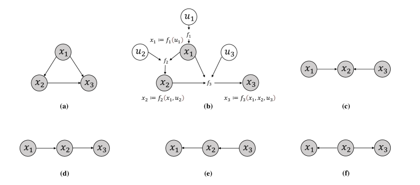
Structural Causal Model (SCM). Pearl’s comprehensive theory of causality, as presented in (Pearl, 2009), enables us to draw causal conclusions from observations using causal hierarchy (PCH) (Pearl and Mackenzie, 2018). From that, the structural causal model is defined as a graphical representation of causal relationships that captures how interventions on one or more variables affect the values of other variables in the data generation mechanism. Formally, SCM can be represented in a 4-tuple , where denote the set of endogenous and exogenous variables respectively, is the distribution of exogenous variables, and represents the set of the mapping function. Specifically, for , the model indicates the assignment of the value to a function of its structural parents and exogenous variable . For each SCM, we can yield a causal graph DAG by adding one vertex for each and directing edges from each parent variable in (the causes) to child (the effect). The relationship of the SCM and the corresponding DAG is shown in figure 2 (a)(b).
d-separation. -separation is a criterion for determining the absence of causal effects between two sets of variables in a graphical model. Two sets of variables are said to be -separated if every path between them is blocked. In formal, a set of variables d-separates two variables if blocks all paths between them. For the given causal graph in figure 2 (d)(e)(f), two vertices are d-separated by the set of vertices if . As for the relations in figure 2 (c) (a.k.a., a v-structure or collider), are also d-separated if and none of the descendants of are in set .
-separation is a fundamental concept in causal discovery because it provides a criterion for determining whether two sets of variables are causally related. If two sets of variables are -separated, then there is no direct or indirect causal effect between them, and they can be considered independent given the observed variables. Conversely, if two sets of variables are not -separated, then there may be a direct or indirect causal effect between them that needs to be accounted for when inferring causal relationships from data. Thus, -separation is an essential tool for identifying causal relationships in graphical models.
Causal Markov Condition. In the causal graph of SCM, each variable is independent of its non-effects given its direct causes (Pearl, 2009). In other words, a variable is conditionally independent of its non-effects (i.e., variables that do not directly cause it) given its parents (i.e., variables that directly cause it). This condition plays an essential role in causal inference. It enables the identification of causal effects from non-experimental data. Formally, the causal Markov condition implies the joint distribution can be factorized according to the following decomposition:
Markov Equivalence Class(MEC). Two graphical models belong to the same MEC if they entail the same set of conditional independence relations among the observed variables, regardless of the specific structure of the graph. For example, the causal diagrams in Figure 2 (d)(e)(f) imply the same d-seperation information and belong to the same MEC. MEC is important because it enables us to identify the minimal set of conditions necessary for inferring causal relationships from non-experimental data.
Causal Identifiability. A causal effect is identifiable if it can be estimated without making any untestable assumptions or invoking additional information beyond the observed variables. This means that all causal graphs in the same MEC represent equivalent causal structures from an observational viewpoint. In general, causal identifiability requires that the causal graph is acyclic and that all backdoor paths between the treatment and outcome variables are blocked. If these conditions are met, the causal effect can be identified using the -calculus or other causal inference techniques. Thus, the prerequisite of causal discovery is that causal relationships can be identifiable.
Causal Minimality. Consider a DAG and a probability distribution , is said to satisfy the causal minimality with respect to if is Markovian with respect to but not to any proper subgraph of . It indicates that all the variables are necessary and sufficient to accurately represent the causal relationships while excluding any variables that do not contribute to the causal mechanism. A distribution is minimal with respect to the causal graph if and only if there is no node that is conditionally independent of any of its parents, given the remaining parents. In other words, all the parents are “active”.
Building on the aforementioned concepts, we introduce three assumptions, causal sufficiency, faithfulness, and temporal priority, which are the untestable foundations of causal discovery.
Causal Sufficiency. A set of variables is causally sufficient if all common causes of all variables are observed (Spirtes et al., 2000). This assumption indicates that the causal graph in SCM can reflect the truth data generation process and there is no hidden confounder. Under the assumption of causal sufficiency, the majority of causal discovery algorithms presume that the causal structure can be depicted as a DAG.
Faithfulness. Faithfulness asserts that all conditional independence relations of that hold in the observed data are entailed by the causal model , and conversely, all conditional independence relations implied by the causal model are also held in the observed data. Note that faithfulness implies causal minimality. If is faithful and Markovian with respect to , then the causal minimality is satisfied.
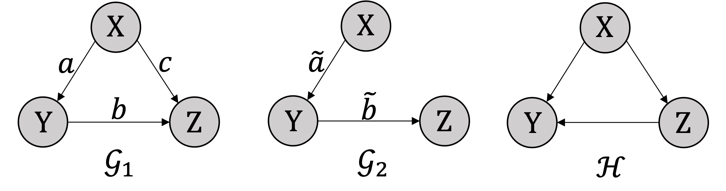
Intuitively, faithfulness is not easy to understand. We try to clarify it with an example (Peters et al., 2017). As shown in Figure 3, we assume the generation process of as a linear Gaussian SCM:
The noise variables , and are jointly independent. Let us consider a special case that . In this setting, the variables and are independent. The direction of would be inverted and the causal model is degraded to . According to the definition, and satisfy the causal minimality. But the faithfulness is violated in this special case, i.e. is not a proper subgraph of . Thus, the probability of this linear Gaussian model is not faithfulness with respective to . Although is a proper subgraph of , the distribution does not satisfy causal minimality because the probability is not Markovian with respect to .
While faithfulness is untestable in practice, it is crucial for deriving valid causal inferences from data because it ensures that the model correctly represents the data-generating mechanisms. If this assumption is violated, the causal relationships are uncertain which is a disaster for causal discovery methods (Spirtes et al., 2000).
Temporal priority. For two variables, temporal priority means that the cause must have occurred before its effect. It is a foundation assumption of causal discovery from temporal data and creates an asymmetric time relationship in causal processes. The temporal priority helps us to establish the direction of a causal relationship when two variables are causally linked. However, if the sampling frequencies of time series are high, the time difference between events associated with the time series may be indistinguishable. In such cases, two events that occurred at different times could be perceived as instantaneous in the observational time series, leading to contemporaneous causal relationships between causes and effects occurring at different time instants.
2.2. Causal Structure for Temporal Data
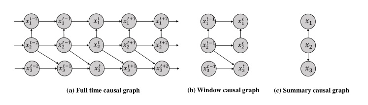
For temporal data, the causal relationship can be intuitively defined by the temporal precedence (Eichler, 2012) indicating the causes precede their effects. It reveals the causality asymmetric in time and can be used to orient a causal relation when two variables are known to be causally related. Based on the temporal precedence, there exist three graphical representations of causal structure, i.e., full-time causal graph, window causal graph, and summary causal graph.
As illustrated in Figure 4 (a), the full-time causal graph represents a complete graph of the dynamic systems. For -variate time series , the measurement at each time point is a vector . Vertices in full-time causal graphs consist of the set of component at each time point with lag-specific directed links such as . However, it’s usually difficult to discover full-time causal graphs due to the single observation for each series at each time point.
To remedy this problem, window causal graph is proposed. It assumes a time-homogeneous causal structure such that the dynamics of observation vector are governed by where the function determines the following observation based on past and the noise . As illustrated in Figure 4 (b), the window causal graph is represented in a time window, the size of which amounts to the maximum lag in the full-time causal graph.
As shown in Figure 4 (c), each time series component is collapsed into a node to form the summary causal graph. The summary graph represents causal relations between time series without referring to time lags (Peters et al., 2013). In many applications, it is sufficient to model the relations between temporal variables without precisely knowing the interaction between time instants.
For causal discovery from temporal data, most works aim to find the summary causal graph. Nevertheless, summary causal graphs do not always correspond to an SCM, which means they do not enable interventional predictions that are consistent with the underlying time-resolve SCM (Janzing et al., 2018; Rubenstein et al., 2017).
2.3. Problem Definitions
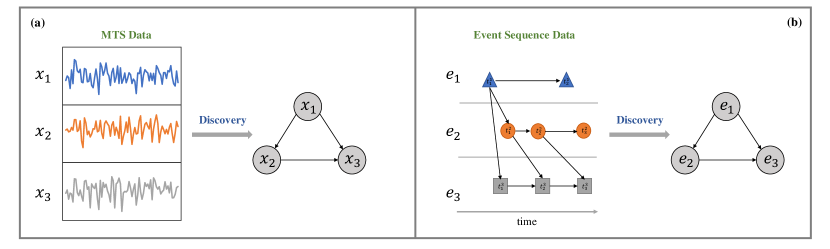
As illustrated in Figure 5, causal discovery from temporal data can be divided into two problems, i.e., causal discovery from MTS and causal discovery from event sequence. Next, we formally define them respectively.
Causal Discovery from MTS. Consider a time series with variables: . Assume that causal relationships between variables are given by the following structural equation model:
where for any at time instance , is the set of direct parents of which can be both in the past and at the same time instance. denotes the independent noise and can denote either measurement noise or driving noise (Peters et al., 2022) without losing generality. Causal discovery from MTS aims to find either of the two kinds of outputs, i.e., summary causal graph or window causal graph. As for the summary causal graph, the output is the adjacency matrix which summarizes the causal structure, and the -th entry of the matrix is if past observations of enter the structural equation of and otherwise. We say that ‘ causes ’ if . As for window causal graph with maximum time lag , the output matrices and correspond to intra-slice and inter-slice edges, respectively. For example, denotes the instantaneous dependency , while denotes a lagged dependency for .
Causal Discovery from Event Sequence. For an event sequence: , indicates the time at which the event occurred, while stands for the corresponding event type. We aim to discover the causal relationships between different event types. In general, we can construct a causal graph , where each node represents a type of event sequence. Our mission is to discover the edge in the causal graph. For example, if there is a directed edge from node to node , we say event-type is a cause of event-type .
3. Causal Discovery from Multivariate Time Series
In this section, we review causal discovery methods for multivariate time-series data, including constraint-based approaches, score-based approaches, functional causal model-based approaches, Granger causality, and others. The representative algorithms combined with the characteristics are summarized in table 3.
| Section | Method | Causal Graph | Nonlinear | Instantaneous effects | Hidden confounders | Sufficiency Asm. | Markov Asm. | Faithfulness Asm. | Minimality Asm. |
|---|---|---|---|---|---|---|---|---|---|
| Constraint-based | oCSE (2015) (Sun et al., 2015) | Summary | Yes | No | No | Yes | Yes | Yes | |
| PCGCE (2022) (Assaad et al., 2022a) | Extended | Yes | Yes | No | Yes | Yes | Yes | ||
| PCMCI (2019) (Runge et al., 2019b) | Window | Yes | No | No | Yes | Yes | Yes | ||
| PCMCI+ (2020) (Runge, 2020) | Window | Yes | Yes | No | Yes | Yes | Yes | ||
| ANLTSM (2008) (Chu and Glymour, 2008) | Window | Yes | Yes | Yes | No | Yes | Yes | ||
| tsFCI (2010) (Entner and Hoyer, 2010) | Window | Yes | No | Yes | No | Yes | Yes | ||
| SVAR-FCI (2018) (Malinsky and Spirtes, 2018) | Window | No | Yes | Yes | No | Yes | Yes | ||
| FCIGCE (2022) (Assaad et al., 2022a) | Extended | Yes | Yes | Yes | No | Yes | Yes | ||
| LPCMCI (2020) (Gerhardus and Runge, 2020) | Window | Yes | Yes | Yes | No | Yes | Yes | ||
| Score-based | DYNOTEARS (2020) (Pamfil et al., 2020) | Window | No | Yes | No | Yes | Yes | No | No |
| NTS-NOTEARS (2021) (Sun et al., 2021) | Window | Yes | Yes | No | Yes | Yes | No | No | |
| IDYNO (2022) (Gao et al., 2022) | Window | Yes | Yes | No | Yes | Yes | No | No | |
| FCM-Based | VAR-LiNGAM (2008) (Hyvärinen et al., 2008) | Window | No | Yes | No | Yes | Yes | No | Yes |
| NCDH (2022) (Wu et al., 2022b) | Summary | Yes | No | No | Yes | Yes | No | Yes | |
| TiMINo (2013) (Peters et al., 2013) | Summary | Yes | Yes | No | Yes | Yes | No | Yes | |
| NBCB (2021) (Assaad et al., 2021) | Summary | Yes | Yes | No | Yes | Yes | Yes333A lighter version of the faithfulness assumption, termed adjacency faithfulness, is needed. | Yes | |
| Granger Causality | HSIC-Lasso-GC (2020) (Ren et al., 2020) | Summary | Yes | No | No | No | No | No | No |
| (R)NN-GC (2015,2018) (Montalto et al., 2015; Wang et al., 2018) | Summary | Yes | Yes | No | No | No | No | No | |
| MPIR (2019) (Wu et al., 2020) | Summary | Yes | No | No | No | No | No | No | |
| NGC (2022) (Tank et al., 2022) | Summary | Yes | No | No | No | No | No | No | |
| eSRU (2020) (Khanna and Tan, 2020) | Summary | Yes | No | No | No | No | No | No | |
| SCGL (2019) (Xu et al., 2019) | Summary | Yes | No | No | No | No | No | No | |
| GVAR (2021) (Marcinkevics and Vogt, 2021) | Summary | Yes | No | No | No | No | No | No | |
| TCDF (2019) (Nauta et al., 2019) | Window | Yes | Yes | Yes | No | No | No | No | |
| CR-VAE (2023) (Li et al., 2023) | Summary | Yes | Yes | No | No | No | No | No | |
| InGRA (2020) (Chu et al., 2020) | Summary | Yes | No | No | No | No | No | No | |
| ACD (2022) (Löwe et al., 2022) | Summary | Yes | No | Yes | No | No | No | No | |
| Others | DBCL (2010) (Voortman et al., 2010) | Summary | Yes | Yes | Yes | No | Yes | Yes | |
| NGM (2022) (Bellot et al., 2022) | Summary | Yes | Yes | No | No | No | No | No | |
| CCM (2012) (Sugihara et al., 2012) | Summary | Yes | No | No | No | No | No | No | |
| PCTL(c) (2009,2011) (Kleinberg and Mishra, 2009; Kleinberg, 2011) | Summary | Yes | No | No | No | No | No | No |
3.1. Constraint-Based Approaches
As a family of causal discovery algorithms, constraint-based approaches rely on statistical tests of conditional independence and are easy to understand and widely used. We first give the main ideas of constraint-based approaches, including general steps and causal assumptions. The detailed methodologies will be categorized into approaches with and without causal sufficiency assumption, and be introduced respectively.
The general steps are: Firstly, it builds a skeleton between variables based on conditional independence. Secondly, it orients the skeleton according to the orientation criterion in the rules. The goal is to construct Completed Partially Directed Acyclic Graphs (CPDAGs) representing the MEC of the true causal diagram. Central to these approaches to derive MEC from observations are the causal assumptions. These methods are usually under the assumptions of causal Markov property and faithfulness, and some also assume causal sufficiency (no unobserved confounders). In this section, we first review the main algorithms and their extensions to time-series data assuming causal sufficiency, then introduce the approaches for conditions when the causal sufficiency assumption is not guaranteed.
3.1.1. Methods with causal sufficiency
In this part, we review methods with causal sufficiency. To reveal the principles of these approaches, we first give a short introduction to methods in the non-temporal setting. Then several popular constraint-based approaches, which originate from the approaches for non-temporal data, for time series are reviewed on the basis of two types of extensions (transfer entropy and momentary conditional independence tests).
As for extracting causal relations from non-temporal data, the Sprites-Glymour-Scheines (SGS) algorithm (Spirtes et al., 1990) is one of the first constraint-based approaches, being proved to be consistent under independently, identically distributed (i.i.d) observations assuming causal sufficiency. However, it suffers from exhausting the test of independence between all nodes. The very large search problem makes it unsuitable in practice. The Peter-Clark (PC) algorithm (Spirtes et al., 2000), which also assumes causal sufficiency, is introduced to reduce unnecessary conditional independence tests and search procedures. Given non-temporal variables, the detailed procedure of PC algorithm is defined as follows in 3 steps: (1) Firstly, the algorithm starts with a completed undirected graph . (2) Secondly, the algorithm respectively retrieves whether there exist pairs of variables and are conditioned on other variables when . If satisfied, remove undirected edges between and , and update the conditioned variables to the separation set. It proceeds to the pruned skeleton. (3) Finally, it determines the collider (V-structure) to obtain the CPDAG and determines the remaining undirected edges based on other rules.
Although approaches such as SGS and PC are designed in non-temporal settings, constraint-based approaches for time-series data are usually extended from them. We will review recent four popular constraint-based methods, which also assume causal sufficiency, for time-series data. Among these methods, two extensions (Sun et al., 2015; Assaad et al., 2022a) are based on the causal concept of Transfer Entropy, another two (Runge et al., 2019b; Runge, 2020) of them are extended to time series via momentary conditional independence tests.
Extension to time series based on Transfer Entropy. Traditional constraint-based approaches can be extended to the scenario of time series based on the concept of Transfer Entropy. The Transfer Entropy is a model-free measure of temporal causality, of which the definition and variants will be detailed in subsection 3.5.1. Here we view the Transfer Entropy measure as an off-the-shelf part and review two representative approaches from the perspective of constraint-based methodology.
The Optimal Causation Entropy (oCSE) Principle (Sun et al., 2015) is proposed to guide computational and data-efficient causal discovery algorithms from MTS data. It’s based on the theoretical concept of Causation Entropy, a generalization of Transfer Entropy for measuring pairwise relations to network relations of many variables The oCSE method takes a procedure slightly different from that in PC: instead of limiting as much as possible the size of its conditioning set, it conditions since the start on all potential causes which constitute the past of all available nodes. The algorithm is summarized in Algorithm 1, which consists of aggregative discovery of causal nodes, and progressive removal of non-causal nodes. In detail, given node , two procedures are conducted jointly to infer its direct causal neighbors: (1) Firstly, it discovers a superset of ’s direct causal neighbors aggregately based on the maximization of Causation Entropy. (2) Secondly, it prunes away non-direct causal neighbors based on the Causation Entropy criterion, for example, is removed from if . It’s a computational and sample-efficient algorithm. However, it assumes that the hidden dynamics follow a stationary first-order Markov process as the Causation Entropy only models causal relations with time lags equal to one. Recently, the PCGCE (Assaad et al., 2022a) is proposed to extract extended summary causal graphs for time-series data based on the PC algorithm and the Greedy Causation Entropy, which is a variant of the Causation Entropy.
Extension to time series via Momentary Conditional Independence Tests. The PCMCI algorithm (Runge et al., 2019b) leverages a variant of the PC algorithm that flexibly combines linear or nonlinear conditional independence tests and extracts causal relations from time-series data. The goal of the algorithm is to discover the window causal graph. Different from that of PC algorithm, PCMCI starts by constructing a partially connected graph, where all pairs of nodes are directed as if . This initialization also caters to temporal priority. The algorithm consists of two stages: (1) As done in PC, PCMCI removes all unnecessary edges based on conditional independence. It furthermore removes homologous edges based on the assumption of consistency through time. (2) Momentary Conditional Independence (MCI) is leveraged to deal with autocorrelation, which may lead to spurious correlation. Here, MCI is a measurement, which conditions on the parents of and while testing . It also provides an interpretable notion of causal strength from to . PCMCI has been shown to be consistent and can be flexibly combined with any kind of conditional independence test (linear or nonlinear), such as partial correlation and mutual information. In recent years, there is also a wealth of machine learning approaches on nonparametric tests that address a wide range of independence and dependence types (Zhang et al., 2011; Runge, 2018).
The PCMCI+ algorithm (Runge, 2020) extends PCMCI to include the discovery of instantaneous causal relations. Central to the PCMCI+ algorithm are two basic ideas that deviate from the origin PC algorithm: First, it conducts the edge removal process separately for lagged and contemporaneous conditioning sets. Second, it leverages MCI to calibrate CI tests under autocorrelation, which is similar to that in PCMCI. The author in (Runge, 2020) also details the curse and blessing of autocorrelation.
3.1.2. Methods without causal sufficiency
Constraint-based approaches without causal sufficiency will be reviewed in this part. In the beginning, we give a brief introduction to the Fast Causal Inference (FCI) Algorithm (Spirtes et al., 2000) for non-temporal data. Then, methods for MTS data consist of two categories: (1) Fast causal inference through time-series models, which is extended from FCI. (2) The methodology via momentary conditional independence tests.
The FCI algorithm is a generalization of the PC algorithm, which can be used in the presence of latent confounders and proven to be asymptotically correct. It utilizes independence tests on the observed data to extract (partial) information on ancestral relationships between the observed variables, thus the goal of the FCI algorithm is to infer the appropriate PAG. The FCI algorithm starts by constructing a complete graph consisting of undirected edges, similar to the PC algorithm. Then iterative conditional independence tests are conducted for the removal of edges. As a result, the FCI algorithm removes edges that are independent, first when conditioning with Sepsets and the with Possible-Dsep sets. For the remaining undirected edges, ten orientation rules are applied recursively. The detailed FCI algorithm, including theoretical analysis, demonstrates the algorithm is sound and complete and can be found in (Zhang, 2008).
Fast Causal Inference Through Time-series Models. A constraint-based method called additive nonlinear time series model (ANLTSM) (Chu and Glymour, 2008) is proposed under the assumption that the effects of hidden confounders are linear and contemporaneous. To escape the curse of dimensionality for nonparametric conditional independence tests, ANLTSM leverages additive regression model, which can be specified as follows :
Here, and are constant values, and denotes the smooth univariate function. The unobserved effects in the form of multi-dimensional Gaussian white noise can be categorized into two types: reflects the latent direct causes of the observed variables, and denotes latent common causes. And the latent common causes affect the observed variables at the same instant. For and , suffices to be stated as a latent common cause if and only if there exists such that . Based on the aforementioned additive regression model, the FCI algorithm is leveraged to identify lagged and instantaneous causal relations. For detecting the instantaneous relations, the conditional independence between and is first tested given the set by estimating the conditional expectation , then the significance of prediction relationship between and is checked using statistical tests such as the F-test or the BIC scores, where the insignificance of the predictor implies the conditional independence between and . The lagged causal relations are identified in a similar way. The remaining edges are oriented based on rules. This method is shown to be consistent if the data generation caters to the additive nonlinear time series models. However, the ANLTSM method restricts contemporaneous interactions to be linear, and latent confounders to be linear and contemporaneous.
Another extension of FCI to time-series data is the tsFCI (Entner and Hoyer, 2010) algorithm, where the FCI algorithm is directly applied via a time window. In detail, by assuming the observed time-series data comes from a system at equilibrium, the original time-series data is transformed into a set of samples of the random vector, via a sliding window of size . Then considering every component of the transformed vector as a separate random variable, the original FCI algorithm is directly applicable. As the amount of information derived from standard FCI is quite restricted, the temporal priority and time invariance is further incorporated as background knowledge to make more inferences in the orientation phase. However, the tsFCI ignores selection variables and contemporaneous causal relations. Recently, a constrain-based approach named SVAR-FCI (Malinsky and Spirtes, 2018) is proposed that allows for both instantaneous influences and arbitrary latent confounding in the data-generating process. Similar to tsFCI, it also uses time invariance to infer additional edge removals.
Methodology Via Momentary Conditional Independence Tests. It’s found that the original FCI algorithm and its temporal variants suffer from low recall in the autocorrelated time-series case due to the low effect size of conditional independence tests (Gerhardus and Runge, 2020). Some researchers aim to extend PCMCI in the presence of unobserved confounding variables to tackle the aforementioned issues. In (Gerhardus and Runge, 2020), the Latent PCMCI (LPCMCI) algorithm is proposed. Central to the LPCMCI algorithm are two ideas that: First, based on the analysis of the effect size in causal discovery, it uses parents of variables as default conditions and non-ancestors are not tested in the condioning sets, which not only avoids inflated false positives but also reduce the sets to be tested. Second, it introduces the notions of middle marks and LPCMCI-PAGs as an unambiguous causal interpretation to facilitate the early orientation of edges. And the LPCMCI algorithm is proven to be order-independent, sound and complete.
3.2. Score-Based Approaches
Another family of causal discovery approaches is based on score function. The main ideas of score-based approaches will first be introduced, including (dynamic) Bayesian Network, characteristics of score-based approaches compared to their constraint-based counterpart, model scoring, and model search. Then, we will review combinatorial search approaches and continuous optimization approaches for MTS, respectively.
3.2.1. Basics of score-based approaches
The score-based approaches are motivated by the idea that graph structures encoding the wrong (conditional) independence will also result in poor model fit. In the score-based approaches, the causal structure is attached to the concept of Bayesian Network (BN) or Dynamic Bayesian Network (DBN) (Dean and Kanazawa, 1989; Murphy, 2002) dealing with temporal data. In light of this, the score-based methods can generate and probabilistically score multiple models, and then output the most probable one. This contrasts with the constrained-based approaches, which derive and output a single model without quantification regarding how likely it’s to be correct. And the faithfulness assumption is diluted in the scored-based approaches by applying a goodness-of-fit measurement instead of a conditional independence test. The problem of learning a BN or DBN from observations can be therefore formulated as: given a set of instances, find the network that best matches them, i.e., optimize the objective functions. It consists of two elements: model scoring and model search.
Model scoring. Common objective functions fall under two categories: the Bayesian scores which focus on goodness-of-fit and allow the incorporation of prior knowledge, and information-theoretic scores which explicitly consider model complexity, aiming to avoid over-fitting, in addition to the goodness-of-fit (Kitson et al., 2021). The family of Bayesian score functions contains Bayesian Dirichlet equivalent (BDe) score (Heckerman et al., 1995), K2 score (Kayaalp and Cooper, 2013), and so on. The most widely used information-theoretic scores include the Bayesian Information Criterion (BIC) (Neath and Cavanaugh, 2012) and the Akaike Information Criterion (AIC) (Burnham and Anderson, 2004).
Model search / Optimization. The score-based approaches cast the problem of searching causal structure into an optimization program using the aforementioned score functions . The ultimate goal is therefore stated as (Peters et al., 2017):
where represents the empirical data for variables . Traditionally, it’s a combinatoric graph-search problem, and the solution is generally sub-optimal as finding a globally optimal network is known to be NP-hard (Chickering, 1995). A line of works, such as Greedy Equivalence Search (GES) (Chickering, 2002) involve local heuristics owing to the large search space of graphs. However, they still suffer from the curse of dimensionality and suboptimal problems. Recently, an algebraic result characterizing the acyclicity constraint is leveraged in structure learning, which turns the combinatoric problems into a continuously optimizing problem (Zheng et al., 2018, 2020), which can be reformulated as:
where denotes the adjacency matrix, and is the function used to enforce acyclicity in the inferred structure. The original acyclicity constraint function is implemented as in (Zheng et al., 2018). It relies on the augmented Lagrangian method (ALM) (Yurkiewicz, 1985) to solve the continuous constrained optimization problem. Various works have further adopted the continuous constrained formulation in neural networks to extract nonlinear causal relations (Zheng et al., 2020; Yu et al., 2019; Gao et al., 2021).
In the context of time series, the ultimate goal of score-based approaches is to learn the structure of DBN. A DBN is a probabilistic network where variables are time series, and it can be decomposed into a prior network and a transition network. A prior network provides dependencies between variables in a given time stamp, and a transition network provides dependencies over time. Therefore, a DBN represents contemporaneous and time-delayed effects in the same framework. Based on this extension to time series, we review the score-based methods following a similar paradigm from combinatoric search to continuous constrained optimization.
3.2.2. Combinatorial search approaches
To conduct the combinatorial search based on scoring function from MTS data efficiently, researches have developed various approaches including structural expectation-maximization (Friedman et al., 1998), cross-validation (Peña et al., 2005), and the decomposition of score functions (de Campos and Ji, 2011).
In (Friedman et al., 1998), the author first utilizes Structural Expectation-Maximization (Structural EM) algorithm (Friedman, 1997, 1998), which is originally a standard algorithm for inferring BN, to learn DBN from longitudinal data. The Structural EM algorithm, combining structural and parametric modification with a single EM process, can be shown to find local optima defined by score functions.
In (Peña et al., 2005), the -fold cross-validation (CV) is leveraged as a computationally feasible scoring criterion for learning DBN. Given the observational data , which is randomly split into folds of approximately equal size, the CV value of a model is formulated as . And a greedy hill-climbing search is used to estimate . The procedure starts from the empty graph and updates it gradually by applying the highest scoring single edge additional or removal available. Experiments show that the scoring methods based on cross-validation lead to models generalizing better than those based on BIC of BDe for a wide range of sample sizes.
Based on the score functions that are decomposable, the paper (de Campos and Ji, 2011) uses structural constraints to cast the problem of structure learning in DBN into a corresponding augmented BN, and presents a branch-and-bound algorithm to guarantee global optimality. The decomposed form of the optimal goal can be formalized as:
where and correspond to the prior network and the transition network respectively. Structural constraints, as a way to reduce the search space, specify where arcs may or may not be included. Because of the branch-and-bound properties, the algorithm can be stopped at the best current solution and an upper bound for the global optimum. The proposed method is shown to be able to handle larger data sets than before, benefiting from the branch-and-bound algorithm and structural constraints.
3.2.3. Continuous optimization approaches
Owing to the recent contribution of NOTEARS (Zheng et al., 2018), the score-based learning of DAGs can be reformulated as a continuous constrained optimization problem, which inspires various works (Zheng et al., 2020; Yu et al., 2019; Gao et al., 2021; Ng et al., 2022b, 2019; Lachapelle et al., 2020) in structure learning. At the heart of this line of the method is an algebraic characterization of acyclicity expressed as a constraint function, which is further leveraged to minimize the least square loss while enforcing acyclicity. In the context of time series, some works have also adopted this continuous constrained formulation to support structure learning and causal discovery (Pamfil et al., 2020; Sun et al., 2021; Hsieh et al., 2021; Gao et al., 2022).
DYNOTEARS, introduced in (Pamfil et al., 2020), captures linear relations from time-series data via a continuous optimization approach. It models the data in the following standard SVAR way:
where is the order of SVAR model, is a vector of centered error variables. To guarantee the identifiability in SVAR models, the error terms are assumed either non-Gaussian or standard Gaussian, i.e., , as the identifiability is proven to hold on the two cases (Hyvärinen et al., 2010b; Peters et al., 2017). and are weighted adjacency matrices, which correspond to intra-slice edges (contemporaneous relationship) and inter-slice edges (time-lagged relationship), respectively. The SEM can further takes the compact form:. The procedure of structure learning revolves around minimizing the least-squares loss subject to an acyclicity constraint, which gives the following optimization problem:
To sidestep the key difficulty of solving the optimization problem under the acyclicity constraint, DYNOTEARS follow the work in (Zheng et al., 2018), where the trace exponential function is leveraged as an equivalent formulation of acyclicity. The continuous constrained optimization problem is translated via the augmented Lagrangian method into unconstrained problems of the form:
Towards the optimization of the above smooth augmented objective, two solving approaches are presented separately. The first approach is to use standard solvers such as L-BFGS-B (Zhu et al., 1997). An alternative approach is a two-stage procedure similar to those in (Hyvärinen et al., 2010b), where we can rewrite the equation as and derive the estimate of by using static NOTEARS to the error term .
NTS-NOTEARS (Sun et al., 2021) is a recent advance that adopts the continuous constrained formulation. Compared to DYNOTEARS, which is a linear autoregressive model, NTS-NOTEARS is able to extract both linear and non-linear relations among variables. It achieves this by leveraging 1D convolutional neural networks (CNNs), which exploit a sequential topology in the input data and are thus well-suited neural function approximation models for temporal data. CNNs, each of which the first layer is a 1D convolutional layer with kernels, are trained jointly where the -th CNN predicts the expectation of targeted variable at the specific time given preceding and contemporaneous input variables. Each CNN can be viewed as a Markov blanket of the target variable. The dependence of child variables on their parents in DBN is given as follows:
where parents are derived from the trained CNNs, and denotes all variables at time step except . In light of NOTEARS-MLP (Zheng et al., 2020) (a non-linear and NN-based extension of NOTEARS), the dependency strength of an edge in DBN is estimated in the following way:
In detail, the belongs to the parent set on the condition that the estimated dependency strength is larger than threshold weight . The optimization procedure follows a similar way as DYNOTEARS. It’s also worth noticing that NTS-NOTEARS shows prior knowledge of variable dependencies that can be transformed as additional optimization constraints and incorporated into the L-BFGS-B solver.
To handle both observational and interventional data, an algorithm, called IDYNO (Gao et al., 2022), is proposed recently. It first introduces a non-linear objective through neural networks to model complex dynamics, then modifies an objective and general solution approach to handle different distributions on intervention targets.
We can find that it’s a powerful methodology for score-based structure learning to use continuous optimization and avoid the explicit combinatoric traversal of possible causal structures. The past several years have also witnessed numerous applications and extensions of this methodology. However, some boundaries and limitations are further discussed in (Kaiser and Sipos, 2022; Reisach et al., 2021; Ng et al., 2022a), including the influence of data scale and the convergence condition of the augmented Lagrangian method. We recommend you take these issues into consideration for further developments and applications of this family of methods.
3.3. FCM-Based Approaches
The two families of methods above either face the inseparability of the MEC or the need for large samples to confirm causal faithfulness. Causal discovery can also be conducted based on Functional Causal Models (FCM) (Pearl et al., 2000), which is also known as SCM in 2.1 and describes a causal system via a set of equations. Recent years have witnessed the proliferation of FCM-based approaches for both temporal and non-temporal data. In this subsection, we first introduce the main ideas of FCM-based approaches, including the functional causal model and the usage of noise in orienting causal relations. Then two families of FCM-based approaches, i.e., methods using independent component analysis and additive noise model, will be reviewed, respectively.
In FCM, each variable is explained by an equation in terms of its direct causes and some additional noise. For example, the function explains the causal link with some additional noise . One basic idea of the FCM-based causal discovery approaches is that statistical noise can be a valuable source of insight, which caters to recent discoveries (Climenhaga et al., 2021) challenging the orthodoxy that the noise should be treated as a nuisance. To be specific, causal relationships can be identified and estimated with the help of noise.
3.3.1. Methods using independent component analysis
In this part, we first introduce the basic idea of this family of methods by reviewing the original algorithm in non-temporal setting (Shimizu et al., 2006). Then, methods for MTS data will be detailed (Hyvärinen et al., 2008, 2010a; Schaechtle et al., 2013; Wu et al., 2022b).
LiNGAM (Shimizu et al., 2006) is a typical FCM-based causal discovery algorithm in non-temporal setting, and has the following assumptions: (1) a linear data generation process, (2) non-Gaussian disturbances, (3) no unobserved confounders. In the LiNGAM model, the relations among observations can be formulated as , where respectively denote the vector of variables, the adjacency matrix of the causal graph and the noise vector. The equation can be rewritten as , where . For the equation, the independent component analysis (ICA) method (Stone, 2004) can be used to estimate , and causal relationships can be derived. Along this line, DirectLiNGAM (Shimizu et al., 2011) further leverages the regression model to ensure the original models to converge to the correct solution in a controlled number of steps. Extensions of LiNGAM to time series are as follows.
As a temporal extension of LiNGAM, VAR-LiNGAM (Hyvärinen et al., 2008, 2010a) estimates the structural autoregressive (SVAR) models by leveraging non-Gaussianity property. SVAR models reflect both instantaneous and time-delayed causal effects and are among the most prevalent tools in empirical economics to analyze dynamic phenomena (Moneta et al., 2013). In VAR-LiNGAM, a representation of time series is a combination of SVAR and SEM, which is defined as:
| (SVAR) |
where is the matrix of the causal effects between the variables with time lag . And are random processes modeling the external influences or ‘disturbances’, which are assumed to be independent, temporally uncorrelated and non-Gaussian. To estimate the above model, a classic least-squares estimation of the autoregressive (AR) model (time lag ) is combined, which is formalized as:
| (VAR) |
Based on the SVAR and VAR formalization, the basic idea of VAR-LiNGAM is that we can estimate of VAR model in a classic least-square fashion consistently and efficiently. And we can deduce the estimate of instantaneous causal effect through LiNGAM analysis. As for the time-delayed effect, it can be derived from reparametrization. The ensuing method in detail is defined as follows in four steps: (1) Firstly, fit the regressions and denote the least-squares estimates of the AR matrices by . (2) Secondly, compute the residuals, i.e., . (3) Thirdly, perform LiNGAM analysis (Shimizu et al., 2006) based on the equation to derive the estimate of instantaneous causal effect . (4) Finally, compute the estimates of the time-delayed causal effect as . The VAR-LiNGAM model degenerates to the LiNGAM model if the order of the autoregressive part is set to zero, i.e., . And an intensive application of this approach in empirical economics can be found in (Moneta et al., 2013).
The VAR-LiNGAM is extended to the identification and estimate of causal models under time-varying situations (Huang et al., 2015), where Gaussian Process regression is further leveraged to automatically model how the causal model change over time. In (Lanne et al., 2017), the initial VAR-LiNGAM is generalized to the condition where the inferred graphs can contain cycles. And the proposed model is demonstrated theoretically to be identifiable. Another algorithm based on LiNGAM, called the Multi-Dimensional Causal Discovery (MCD), is proposed in (Schaechtle et al., 2013). MCD can efficiently discover causal dependencies in multi-dimensional settings, such as time-series data, by integrating data decomposition and projection.
To get rid of constraints of linear (Hyvärinen et al., 2008, 2010a) or additive assumptions(Peters et al., 2013), an FCM-based algorithm named Nonlinear Causal Discovery via HM-NICA (NCDH) is recently proposed in (Wu et al., 2022b) to extract general nonlinear relations from time series. At the heart of this algorithm, a nonlinear ICA algorithm is leveraged as a measurement of nonlinear relationships. The observations are assumed to be generated by mutually independent latent components:
Similar to that in linear ICA, contains components that are independent of each other, and the goal of nonlinear ICA is to recover from . NCDH first leverages the nonlinear ICA combined with HMM (Hälvä and Hyvärinen, 2020) to separate latent noises. As a remedy for the permutation uncertainty of ICA, a series of independence tests are conducted to determine the corresponding relations between the observed variables and the separated noises. A recursive search algorithm is finally taken to extract the causal relations.
3.3.2. Methods using additive noise model
In reality, there’re many non-linear causal relationships that violate the assumption of LiNGAM family methods. Despite recent advances (such as NCDH) extracting causal relations in general nonlinear conditions, their usages are restricted. Another family of FCM-based approaches is based on the additive noise model (ANM) with nonlinear function, which is suitable in more general settings. In this part, the main ideas of methods using ANM will be given firstly. Then we will introduce the detailed methods for MTS data.
It’s demonstrated in (Hoyer et al., 2008) that the true causal structure can be identified in the ANM with nonlinear functions if the causal minimality condition holds. In ANM, if , we have , and the cause and additive noise are independent. If the noise is subject to non-Gaussian distribution and is a linear function. In the bivariate case , we can fit regression models in causal and anti-causal directions, the true orientation can be inferred by testing the independence with residuals. As for the multivariate case, a pairwise strategy can be adopted (Mooij et al., 2009). The correctness of this algorithm is discussed in (Peters et al., 2014).
In (Peters et al., 2013), the Time Series Models with Independent Noise (TiMINo) is proposed, which is a causal discovery method for time series based on ANM. It inputs time-series data and outputs either a summary time graph or remains undecided, which avoids leading to wrong causal conclusions when the model is mis-specified or the data is insufficient. It leverages a similar method as that in non-temporal and multivariate setting (Mooij et al., 2009). In detail, it tries to fit the structural equation models for time series, which can be formulated as follows:
where error terms are jointly independent over variable index and time index . There are several options for fitting methods such as linear models, generalized additive models, and Gaussian process regression models. For inferring causal relations in the additive noise model, independence tests such as cross-correlations and HSIC (Gretton et al., 2007) can be leveraged.
There are some drawbacks to those functional causal models, such as VAR-LiNGAM and TiMINo. It’s illustrated that those methods are not well scalable across the increase of node numbers (Glymour et al., 2019), and those performances are not promising without a large sample size (Malinsky and Danks, 2018). To overcome those drawbacks, a Noise-Based / Constraint-Based (NBCB) approach is proposed in (Assaad et al., 2021), where the constraint-based approach is further leveraged based on the original additive noise model for time-series data. In detail, the potential causes of each time series are detected by an additive noise model which is similar to that in TiMINo. Unnecessary causal relations are pruned using temporal causal entropy, which is an extension to causation entropy (Sun et al., 2015) measuring the (conditional) dependencies between two-time series.
3.4. Granger Causality Based Approaches
Granger causality is a popular tool for analyzing time-series data in many real-world applications. There exist many causal discovery approaches developed on the basis of Granger causality. In this subsection, we first introduce definitions of Granger causality. Before delving into detailed methods, two categories of Granger causality models for MTS (model-free and model-based) will be given and compared. Due to the superiority of model-based approaches in more general conditions, the rest of this part will focus on two recent advances in model-based approaches: (1) methods based on kernels (3.4.3), and (2) methods based on neural networks (3.4.4).
3.4.1. Basics of Granger causality
Granger causality analysis, which is first proposed in (Granger, 1969), is a powerful method that determines cause and effect based on predictability. A time series Granger-causes if past values of provide unique, statistically significant information about future values of . According to this proposition, is defined to be ‘causal’ for if
where denotes the optimal prediction of given the history of all relevant information . Here indicates excluding the information of from . The above definition seems general and does not have specific modeling assumptions, whereas there are also various forms of definition for Granger causality based on different model specifications and statistical tools for better representation power and the convenience of inference, such as autoregression model (in Granger’s original paper (Granger, 1969)) and so on. And if all relevant variables are observed and no instantaneous connections exist, Granger causal relations are equivalent to causal relations in underlying DAGs (Peters et al., 2013, 2017).
3.4.2. Early approaches for MTS
Earlier methods for identifying Granger causality were limited to bivariate settings. Specifically, a well-documented (Lütkepohl, 1982) issues for Granger causal analysis in bivariate settings is that the causal findings may be misleading without adjusting for all relevant covariates. On the one hand, it’s necessary to account for more variables to prevent identifying incorrect Granger causal relations (Shojaie and Fox, 2021). On the other hand, MTS widely exist among various fields. Inferring Granger causal relations in MTS, which is also termed graphical Granger causality or network Granger causality in some literature, has become a hot research topic. Various graphical Granger causal analysis models for MTS can be divided into two categories, namely model-free and model-based approaches.
Model-free Methods. The mainstream of model-free approaches for multivariate Granger causality are based on predictability and need to estimate the conditional probability density functions (CPDFs) (Bai et al., 2010). In (Diks and Wolski, 2016), the estimates of the CPDFs are provided, and the the bivariate Diks-Panchenko nonparametric causality test is extended to the multivariate case. By introducing conditional variables into the marginal probability density functions, the copula-based Granger causality model (Hu and Liang, 2014; Kim et al., 2020) can also be extended to multivariate case. Besides, model-free measures such as transfer entropy and directed information (Amblard and Michel, 2011), are able to detect nonlinear dependencies. The definitions and some properties of these model-free estimators will be detailed in 3.5.1. Model-free methods can deal with nonlinear Granger causal relations well. However, these estimators suffer from high variance and require large amounts of data for reliable estimation, and also suffer from curse of dimensionality when the number of variables grows. Thus, in the complex real-word scenarios where is nonlinear and high-dimensional, the utilization of model-free methods to some extend are limited.
Model-based Methods. In contrast to model-free counterparts, model-based methods are computationally efficient and therefore more suitable for inferring Granger causal relations in high-dimensional conditions. The model-based inference approach is adopted by the vast majority of Granger causal whereby the measured time series is modeled by a suited parameterized data generative model. And the inferred parameters ultimately reveal the true topology of Granger causality. Earlier methods along this line are typically using the popular vector autoregressive (VAR) model under the assumption of linear time-series dynamics. For -variate time series , the VAR model is defined as:
where is a matrix that specifies how lag affects the future evolution of the series and denotes zero mean noises. In the VAR model, as a straightforward extension form the bivariate case (Granger, 1969), time series does not Granger-cause time series if and only if for all time lag , the component of equals zero. Thus the Granger causal analysis reduces to determine which entries in are zero over all lags. There are also abundant research works (Arnold et al., 2007; Lozano et al., 2009a; Shojaie and Michailidis, 2010; Basu et al., 2015) reducing the computational complexity via the Lasso penalty and its variants for Granger causal analysis in high-dimensional time series, which are also termed as Lasso Granger causality (Lasso-GC). For these methods, the problem of Granger causal series selection can be generally formulated as follows based on least square loss:
where is the sparsity-inducing regularizer and has various implementations as shown in table 4. Different penalty terms induce different sparsity patterns in , thus inducing different heuristics and constraints in the Granger causal series selection. Except for Lasso-GC, another line of works based on VAR models in multivariate setting worth mentioning is the conditional Granger causality index (CGCI) (Geweke, 1982). For variable and conditional variables , by comparing residuals errors of the reduced and full models , a distinction between direct and indirect causality in multivariate systems can be made based on CGCI. Along this line of works, mBTS-CGCI is proposed in (Siggiridou and Kugiumtzis, 2016) based on a modified backward-in-time selection (mBTS) to limit the order of VAR models, thus can be better applied to high-dimensional scenarios.
| Model Structure | Penalty Function |
|---|---|
| Basic Lasso | |
| Elastic net | |
| Lag group Lasso | |
| Component-wise Lasso | |
| Element-wise Lasso | |
| Lag-weighted Lasso |
Although the model-based approaches, compared to the model-free counterparts, take advantage of efficiently processing high-dimensional time series, the fundamental issue of these approaches is the model misspecification. Especially, the notion of multivariate Granger causality based on the vanilla VAR model assumes time series follows linear dynamics, whereas many interactions in real-world applications are inherently nonlinear. Recently, many model-based approaches, which are compatible with nonlinear causal relations, have emerged and can be grouped into two categories: methods based on kernel, and methods based on neural networks. As the generation on Granger causality, fundamental venation and development orientations have been reviewed above and prospected from classic documents. In the following part of this subsection, due to their ability to be leveraged in complex real-world scenarios, we will detail the recent advances of model-based methods in nonlinear and high-dimensional settings, especially new perspectives from neural networks.
3.4.3. Recent advances based on kernels
To extract nonlinear causal relations in a model-based approach, establishing a nonlinear parameter model is a common strategy. A line of works extend Granger causality to kernel methods (Ancona et al., 2004; Marinazzo et al., 2008b, a; Sindhwani et al., 2013; Ren et al., 2020). In (Ancona et al., 2004), Granger causality is extended to bivariate nonlinear cases by means of radial basis functions. Furthermore, a Granger causality analysis model is put forward (Marinazzo et al., 2008b) based on the theory of reproducing kernel Hilbert spaces (RKHS). The key idea is to embed data into a Hilbert space and search for nonlinear relations in that space. This method is then generalized to the multivariate case in (Marinazzo et al., 2008a). In (Sindhwani et al., 2013), a matrix-valued extension of the kernel method is proposed, imposed on a dictionary of vector-valued RKHS. The algorithm is for high-dimensional nonlinear multivariate regression, and can naturally lead to nonlinear generalization of graphical Granger Causality. Recently, an algorithm based on Hilbert-Schmidt independence criterion Lasso Granger causality (HSIC-Lasso-GC) (Ren et al., 2020) is proposed.
3.4.4. Recent advances based on neural networks
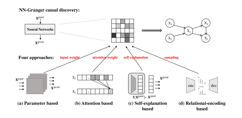
Neural networks are able to represent nonlinear, complex, and non-additive interactions between variables. In this part, recent advances of Granger causal methods based on neural networks will be reviewed, including non-uniform embedding (Montalto et al., 2015; Wang et al., 2018), information regularization (Wu et al., 2020), component-wise neural network modeling (Tank et al., 2017, 2022; Khanna and Tan, 2020), low-rank approximation (Xu et al., 2019), self-explaining networks (Marcinkevics and Vogt, 2021), attention mechanisms (Nauta et al., 2019; Schwab et al., 2019), recurrent variational autoencoders (Li et al., 2023), and inductive modeling (Chu et al., 2020; Löwe et al., 2022). Besides, as illustrated in Fig 6, existing NN-based Granger causality approaches can be categorized into four groups: parameter-based (Tank et al., 2022; Khanna and Tan, 2020), attention-based (Nauta et al., 2019; Chu et al., 2020), self explanation-based (Marcinkevics and Vogt, 2021), and relational encoding-based (Löwe et al., 2022).
DL-extensions with Non-uniform Embedding. A feature selection procedure termed as a non-uniform embedding (NUE) is proposed in NN-GC (Montalto et al., 2015) to identify the significant Granger causes in the MLP model. By greedily adding lagged components of predictor time series as input, an MLP is updated iteratively. A predictor time series is claimed a significant Granger cause of the target time series if at least one of its lagged components is added when the procedure is terminated. In RNN-GC (Wang et al., 2018), the NUE is extended by replacing MLPs with gated RNN models, However, as this technique requires training and comparing many candidate models, it’s costly in high-dimensional settings.
DL-extensions with Information Regularization. For extracting nonlinear dynamics, a method with Minimum Predictive Information Regularization (MPIR) (Wu et al., 2020) is introduced. It leverages learnable corruption for predictor variables and minimizes a mutual information-regularized risk, which combines the benefits of the Granger causality paradigm with deep learning models. In MPIR, the author states that the naive way to combine neural nets with Granger causality suffers from two major drawbacks: instability and inefficiency. The solution is to encourage each to provide as little information to as possible while maintaining good prediction via learned corruption, replacing the naive way which predicts with one missing at a time. The risk is defined as follows:
where (or its element-wise representation, ) are the noise-corrupted inputs with learnable noise amplitudes and . And is the minimum predictive information at the minimization of , which contains causal information and measures the predictive strength of variable for predicting variable , conditioned on all the other observed variables. To be specific, if . Besides, as it’s inefficient to estimate the mutual information term with a large dimension, an upper bound is derived as an alternative optimization goal. Instead of training many candidate models and suffering from instability and inefficiency, this framework only requires training models separately.
DL-extensions with Component-wise NN Modeling. Another NN-based approach to measure nonlinear Granger causality is component-wise modeling. A component-wise framework is proposed in (Tank et al., 2017), which can be viewed as a generalization of the linear VAR model. In detail, the generation procedure of each variable can be written as follows:
where is a continuous function, based on regularized neural networks implementation, specifying how the past values of determine the future values of variable . In this context, the time series is Granger non-causal for time series () if and only if is invariant to , which can be defined as:
for all and all . We will introduce two methods (Tank et al., 2022; Khanna and Tan, 2020) based on this framework, respectively.
Neural Granger Causality (NGC) is proposed in (Tank et al., 2022) to infer nonlinear Granger causality using structured MLP and LSTM with sparse input layer weights, which are termed as component-wise MLP (cMLP) and component-wise LSTM (cLSTM), respectively. In the cMLP, each nonlinear output is modeled with a separate MLP as to easily disentangle the effects from inputs to outputs. The input matrix of the first layer provides information for penalized selection of Granger causality. To be specific, in the first layer of
if the -th column of weight matrix contains zeros for all time lag , then time series does not Granger-cause series . Analogously to the VAR type methods, the Granger causal series are selected by the following encoding selection(Tank et al., 2017) procedure:
where sparse inducing penalty is implemented through group lasso penalty, which extracts causal relations without requiring precise lag specification. As for the cLSTM, it sidesteps the lag selection problem and the Granger causal information can also be easily interpreted in the vanilla LSTM model. The input matrix, which is slightly different from that in MLP, is defined as , controlling how the past time series affect the forgot gates, input gates, output gates, and cell updates. Granger-causal series can be selected based on a group lasso penalty across columns of . In the end, to optimize the non-convex optimization objectives in either cMLP or cLSTM, the proximal gradient descent(Parikh et al., 2014) is used, which leads to the exact zeros in the input matrix. This property in the optimization procedure meets the requirement for interpreting Granger non-causality in the framework. To infer the network topology of Granger causality, models need to be trained with each variable as a response.
Another sample-efficient architecture economy-SRU (eSRU) is proposed in (Khanna and Tan, 2020). It leverages Statistical Recurrent Units (SRUs) (Oliva et al., 2017) to model the observed time-series data. Here SRUs are a special type of RNNs designed for MTS with time-delayed and nonlinear dependencies and therefore also suited for extracting the network topology of nonlinear Granger causal relations. To be specific, it suffers less from the vanishing and exploding gradient issues owing to an ungated architecture and is able to model both short and long-term temporal dependency among multivariate time series by maintaining multi-time scale summary statistics. Similar to model-based approaches like cLSTM, the measure of Granger causal relationships can be derived from the input-layer weight parameters of the SRUs. However, due to the common issue of data scarcity in the causal inference problem, the original framework suffers from overfitting. Additionally, two modifications are implemented as a remedy for overfitting in eSRU.
DL-extensions with Low-rank Approximation. The scalable causal graph learning (SCGL) framework is proposed in (Xu et al., 2019). The authors first deconstruct data nonlinearity into two types (i.e. univariate-level and multivariate-level nonlinearity), which are modeled separately. The key idea of SCGL is that learning the full size of the adjacency matrix would be unscalable when the size of variables is quite large. In practice, the relationship of variables is low-rank in hidden space (Zorzi and Chiuso, 2017; Chiuso and Pillonetto, 2012). Therefore, it’s natural to approximate via a -rank decomposition, where . The low-rank approximation reduces the noise influence in causal discovery and provides interpretability in downstream time series analysis (Huang et al., 2020c).
DL-extensions with Self-explaining Networks. For better interpretability, the generalized vector autoregression (GVAR) model (Marcinkevics and Vogt, 2021) is proposed. It’s based on an extension of self-explaining neural networks (Alvarez-Melis and Jaakkola, 2018). The self-explaining neural networks are inherently interpretable models motivated by restricted properties, and follow the form:
where and denote a link function and the interpretable basis concepts, respectively. Combined with the vector autoregression model, which is often specified in Granger causal inference, the GVAR model is given by
where is a neural network parameterized by , of which the output is the matrix corresponding to the strength of influence. In detail, the strength of influence is measured by the component of . The loss function consists of three terms: the MSE loss, a sparsity-inducing regularization (can be chosen from 4), and the smooth penalty, which is defined as follows:
here is the observed d-variate time series whereas is the one-step forecast made by the GVAR model. Now that the interpreting matrices for each time point can be derived via , the signs of Granger causal effects and their variability in time can also be assessed. Furthermore, a procedure of GVAR based on the heuristics of time-reversed Granger causality (Winkler et al., 2016), which expects the relationships to be flipped on time-reversed data, is leveraged to improve the stability of the inferred structures. Compared to the aforementioned methods, such as cMLP, cLSTM, eSRU and MPIR, another key difference is that these methods require training neural networks, whereas GVAR requires training networks.
DL-extensions with Attention Mechanisms. The temporal causal discovery framework (TCDF) is introduced in (Nauta et al., 2019), which utilizes attention-based dilated CNN. This framework consists of independent attention-based CNNs with the same architecture but different target variable . For each target variable, a neural network is proposed to derive prediction, attention scores and kernel weights. Intuitively, a high attention score on while forecasting indicates the former contains prediction information towards the latter. A permutation-based procedure is additionally provided for evaluating variable importance and identifying significant causal links. TCDF can discover self-causation and time delays between cause and effect. Besides, by assuming that the bidirectional causal relations can not be instantaneous, it can also detect the presence of hidden confounders with equal delays.
Besides, an interpretable multi-variable LSTM with mixture attention is proposed in IMV-LSTM (Guo et al., 2019, 2018) to extract variable importance knowledge. And it’s widely used as a baseline for causal discovery in multivariate time series. However, the topic on attention and its interpretation is to some extent still a controversial and inconclusive topic (Jain and Wallace, 2019; Wiegreffe and Pinter, 2019; Grimsley et al., 2020). Especially in the context of Granger causal explanation, the naive-trained soft attention mechanisms are noted (Sundararajan et al., 2017; Schwab et al., 2019; Chu et al., 2020) to provide no incentive to yield accurate attributions. In (Schwab et al., 2019), Granger causal attention weights are introduced based on the measures named as the mean Granger-causal error. The decrease in error when adding can be computed as:, given the auxiliary prediction error with and without any information from the -th variable. Then the Granger-causal attention factor can be computed as:. The attention factor is able to capture Granger causality, which is zero if -th time series is Granger noncausal for the target series.
DL-extensions with Recurrent Variational Autoencoders. Recently, the causal recurrent variational autoencoder (CR-VAE) (Li et al., 2023) is proposed, where a generative model incorporates Granger causal learning into the data generation process. By preventing encoding future information before decoding, the encoder of CR-VAE obeys the principle of Granger causality To be specific, given time lag , a CR-VAE model can be written as:
where represent encoder and decoder. Another distinct to the classical recurrent VAE is that the CR-VAE leverages a multi-head decoder where the -th head is designed for generating . Besides, an error-compensation module is leveraged to capture instantaneous effects. The CR-VAE is not only able to extract causal relations, but also conduct the data-generating process in a transparent manner benefiting from the learned causal matrix.
DL-extensions with Inductive Modeling. The problem of methods with inductive modeling is slightly different from the above methods, where MTS data from massive individuals, which entails different causal mechanisms but shares common structures, is collected. The goal is to train a model on samples with heterogenous structures to discover Granger causal relations from each individual. Two approaches with inductive modeling are reviewed here.
An inductive Granger causal modeling (InGRA) is proposed in (Chu et al., 2020), combined with Granger causal attention (Schwab et al., 2019) and prototype learning. As there often exist real-world scenarios where massive multivariate time series data is collected from heterogeneous individuals sharing commonalities. Instead of training one or a set of models for each individual, InGRA trains a global model for individuals potentially having different Granger causal structures, devoid of sample inefficiency and over-fitting issues. Firstly, the Granger causal attention mechanism is leveraged to quantify variable-wise contributions toward prediction. As the Granger causal attention is not robust enough to reconstruct Granger causal topology from limited data of a single individual, InGRA secondly leverages prototype learning, of which the key idea is to solve problems for new inputs based on similarity to prototypical cases, to detect common causal structures. As a result, the Granger causal relations and strengths between the exogenous variables and the target variable are inferred.
A framework termed amortized causal discovery (ACD) is proposed in (Löwe et al., 2022), which aims to train a single model to infer causal relations across samples with different underlying causal graphs but shared dynamics. It’s an encoder-decoder framework, in which the encoder function is defined to infer Granger causal relations of the input sample whereas the decoder function learns to predict the next time-step given the inferred causal relations. In the implementation, a graph neural network is applied to the amortized encoder, and ACD models the functions using variational inference, which is based on the widely used neural relational inference (NRI) model (Kipf et al., 2018). Besides, to derive a causal interpretation of the inferred edges, the proof is provided in ACD to relate the zero-edge function to Granger causality. As a result, the causal relations of previous unseen samples can be inferred without refitting the model.
3.5. Others
The aforementioned four categories of approaches have been the subjects of many endeavors in causal discovery research. For the sake of completeness, we present five types of methods that are distinct from the above approaches in this subsection, including causality based on information-theoretic statistics, causal models based on differential equations, nonlinear state-space methods, logic-based methods, and hybrid methods.
3.5.1. Causality based on information-theoretic statistics
Causal relationships in MTS can be measured based on information-theoretic statistics. As a model-free measure, it’s widely used in constraint-based approaches (3.1.1) and Granger causal models (3.4.2). However, its definitions and characteristics have not been detailed. In this part, we will first introduce Transfer Entropy (Schreiber, 2000), which is the original concept of information-theoretic statistics of causality, and then its variants.
Transfer Entropy (Schreiber, 2000) is a measure of information flow or effective coupling between two processes, regardless of the actual functional relationship. Instead of model-based criterion, which shares the problem that the model might be misspecified, as a model-free measure, it can be combined with a variant of specific structure learning methods. In detail, the Transfer Entropy from to (with time lag) can be expressed as:
where denotes the conditional entropy. Here the term measures the uncertainty of given information about , and measures the uncertainty of given information about both and . Therefore, we can understand Transfer Entropy in the causal view of reduction of uncertainty about future dynamics of when the current dynamics of is given addition to that of . For Gaussian variables, the equivalence between Transfer Entropy and Granger causality is demonstrated in (Barnett et al., 2009). Furthermore, Transfer Entropy is reformulated into a decomposition form and embedded into the framework of graphical models for multivariate in (Runge et al., 2012b). In (Runge et al., 2012a), the causal coupling strength for multivariate time series is quantified based on a variant of transfer entropy.
Although some utilization in multivariate scenarios, Transfer Entropy suffers from the pairwise limitation. And it’s reported to fail to distinguish between direct and indirect causality in networks (Sun et al., 2015) . As a remedy to pairwise limitation, Causation Entropy (Sun and Bollt, 2014), a model-free information theoretic statistic for inferring causality, is introduced. In detail, the Causation Entropy from the set of nodes to the set of nodes conditioning on the set of nodes is defined as follows:
here are all subset of nodes . As a type of conditional mutual information, Causation Entropy is a generalization of Transfer Entropy for measuring pairwise relations to network relations of many variables. And similar to the equivalence relations between Transfer entropy and Granger Causality, Causation Entropy also generalizes Granger Causality and Conditional Granger Causality when applied to Gaussian variables. However, according to its definition, this concept assumes that the hidden dynamics follow a stationary first-order Markov process as the Causation Entropy only models causal relations with time lags equal to one. Recently, to measure any lagged or instantaneous relations, an extension of Causation Entropy, named Greedy Causation Entropy, is proposed in (Assaad et al., 2022a).
3.5.2. Causal models based on differential equations
Differential equations are a commonly used modeling tool in many fields, and are especially useful if measurements can be done on the relevant time scale. Compared to the aforementioned causal models, this type of approach is specifically designed to model systems that can be well represented by differential equations (Peters et al., 2022). In this part, we will first review the relationships between differential equations and causal models, for both discrete and continuous time. The first difference-based causal discovery framework will be introduced. Then, we will give the recent advances in this type of method.
There is abundant literature (Peters et al., 2022; Bongers et al., 2018) (Schölkopf, 2019; Mooij et al., 2013; Rubenstein et al., 2018) discussing the relationship between differential equations and structural causal models. For discrete time, a difference-based causal discovery framework is first proposed in (Voortman et al., 2010). The cross-temporal restriction is satisfied, where all causation across time is due to a derivative causing a change in its integral . This characteristic makes the difference-based causal model a restricted form of dynamic SEMs. And difference-based causality learner (DBCL) is leveraged to extract difference-based causal models from data, which is proven to be able to identify the presence or absence of feedback loops. For continuous time, several theoretical endeavors have also been made to derive a causal interpretation of dynamic systems by both ordinary differential equations (ODEs) (Mooij et al., 2013; Rubenstein et al., 2018; Blom et al., 2019; Pfister et al., 2019) and stochastic differential equations (SDEs) (Hansen and Sokol, 2014; Mogensen et al., 2018).
More recently, under a dynamic causal system where the multivariate time series are irregularly-sampled (in infinitesimal interval of time), an algorithm called neural graphical model (NGM) is proposed in (Bellot et al., 2022). In many applications, the underlying causal system of interest can be represented as a dynamic structural model as follows:
where is a -dimensional standard Brownian motion, is a Gaussian random variable independent of , and the function describes the causal graph . NGM is a learning algorithm based on penalized Neural Ordinary Differential Equations (neural-ODE). The recovery of causal graph can be cast to penalized optimization problems of the form:
where the observation of the systems are at irregular time points .
3.5.3. Nonlinear state-space methods
In this part, we will first introduce the basics of nonlinear state-space methods, including the Takens theorem and Convergent Cross Mapping algorithm. Then variants and recent advances of the original algorithm will be given, to tackle the challenges such as high sensitivity to noise, large sample demands, inconsistent results, and misidentifications.
The state space reconstruction theory proposed by Takens (Takens, 1981) provides a theoretical basis for analyzing the dynamic characteristics of nonlinear systems. Based on this theory, another approach for determining causality, known as Convergent Cross Mapping (CCM), was first proposed in (Sugihara et al., 2012). Developed for coupled time series, this method leverages Takens’ theorem via state space reconstruction. In detail, given two time series and , the attractor manifolds are first reconstructed using and , respectively. Secondly, causality can be detected by measuring the correspondence between and , to be specific, by testing whether every local neighborhood defined on one manifold is preserved in the other. Figure 7 gives the illustration of CCM. This methodology has been successfully applied in many fields (Hirata et al., 2016; Ye et al., 2015) where nonlinear systems are dynamically coupled.
However, there exist issues for the original CCM method, such as high sensitivity to observation noise, a requirement for a relatively large number of observations, and inconsistent results under different optimal algorithms. To overcome these challenges, variants of CCM based on time-lagged analysis (Ye et al., 2015), deep Gaussian process (Feng et al., 2019) reservoir computing (Huang et al., 2020b) and neural ODE (Brouwer et al., 2021) were proposed. Besides, most CCM-based approaches have been originally developed for bivariate analysis. Although the same procedures may be used multiple times to ascertain the causal network among multivariate time series, the performance is not guaranteed under high-dimensional conditions (Huang et al., 2020a). Misidentifying indirect causations as direct ones performs one of the key challenges in multivariate settings. Recently, partial cross mapping (PCM), which combines CCM with partial correlation, was proposed (Leng et al., 2020) to eliminate indirect causal influences.
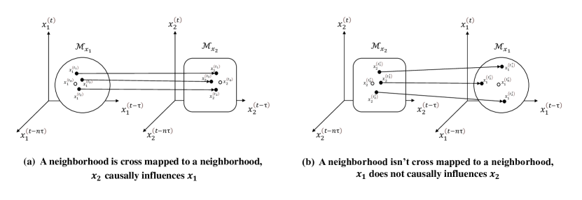
3.5.4. Logic-based methods
Another type of methodology, used for causal inference and causal discovery in time-series data, is based on logic formulas. The original algorithm of this type of approach will first be introduced and combined with its semeiology and definition of potential causality. Then we will give its variants and recent advances.
In logic-based methods, temporal data can be thought of as observations of the sequence of states the system has occupied and is referred to as traces in model checking. This line of research originates from work in (Kleinberg and Mishra, 2009), where causal relationships are described in terms of temporal logic formulas. To be specific, it first leverages logic, Probabilistic Computation Tree Logic (PCTL), to define prima facie (potential) causality based on temporal priority and the uplift of conditional probability. Given the notation in the original work, the prima facie cause is defined if the following conditions all hold: (1) , (2) , and (3) , implying that there may exist any number of transitions between and and the sum of a set of path probabilities are at least . To separate the underlying prima facie (potential) causes into genuine and spurious causes, the notion of -insignificant cause is introduced by computing the average difference in probabilities for each prima facie cause of an effect in relation to all other prima facie causes of the effect:
where . A prima facie cause is an -insignificant cause of if . The value of is chosen based on empirical null hypothesis testing by assuming: (1) data contains two classes, significant and insignificant, (2) the significant class is relatively small to the insignificant class. And false discovery rate control is implemented simultaneously. This methodology has also applications in fields (Kleinberg, 2013).
To expand the methodology to the condition where both discrete and continuous components exist, PCTLc is introduced in (Kleinberg, 2011) to express temporal and probabilistic properties involving discrete and continuous variables, and the significance of relationship in the continuous case is validated via conditional expectation of an effect instead of conditional probability. Besides, a variant (Huang and Kleinberg, 2015) of this logic-based approach was proposed to improve the accuracy of causal discovery and enable faster computation of causal significance, by showing the computational complexity can be reduced under several conditions. Following this line of temporal logic form, a recent work (da Costa and Dasgupta, 2021) combines the idea of decision trees and reconsiders the problem of causal discovery to extract temporal causal sequence relationships from real-time time series.
3.5.5. Hybrid methods: combining score-based and constraint-based approaches
Hybrid approaches are proposed for the benefit of combining the strengths of both constraint-based (3.1) and score-based (3.2) approaches. We cover two parts of hybrid methods, including methods based on max-min hill-climbing heuristics, and methods incorporating the conditional independence tests to improve the local search.
Some researchers develop hybrid approaches based on max-min hill-climbing heuristics (Tsamardinos et al., 2006; Li and Ngom, 2013; Li et al., 2016). As hybrid local learning methods, Max-Min approaches fuse concepts from both constraint-based techniques to limit the space of potential structures and search-and-score Bayesian methods to search for an optimal structure. They are originally leveraged in the structure learning of BN for static data (Tsamardinos et al., 2006). The Max-Min hill-climbing Bayesian network (MMHO-DBN), introduced in (Li et al., 2016), learns the structure of DBN based on an extension of the max-min hill-climbing heuristic and is leveraged in the modeling of real gene expression time-series data.
There are also hybrid approaches that combine conditional-independence tests and local search to improve the criterion score (Ogarrio et al., 2016; Malinsky and Spirtes, 2018). Greedy FCI (GFCI) (Ogarrio et al., 2016) is a hybrid score that combines features of GES with FCI. SVAR-GFCI (Malinsky and Spirtes, 2018) extends this method to causal structure learning from time series. In (Sanchez-Romero et al., 2019), both a variant of the PC-stable algorithm referred to as Fast Adjacency Skewness (FASK), and a hybrid two-step algorithm is proposed for extracting causal relations for time-series data.
4. Causal Discovery from Event Sequences
An important assumption in multivariate time series is that the timestamps are discrete and the time intervals are fixed. However, in the real-world scenario, the vast majority of events will not occur at fixed intervals. In consequence, we need to come up with some methods to deal with these irregular and asynchronous data. We can construct event sequences as , where the first dimension represents the time at which the corresponding event happens, and the second dimension stands for the corresponding event type. In this section, we will focus on inferring causal relationships in event sequences. First, the multivariate point process is introduced, which is preliminary for causal discovery in event sequences. Then, we review approaches based on the Granger causal model, which are well-developed. Lastly, other approaches including constraint-based and score-based methods are given.
4.1. Multivariate Point Process
An event sequence records the occurrence of one specific type of event (or ‘event type’ for simplicity). Meanwhile, we can characterize an event sequence through a point process. To discover the relationships between different types of events, we consider its high-dimensional cases, which is to model event sequences through Multivariate Point Processes (MPPs). Therefore, our problem can be defined as inputting a set of point processes, where each point process represents an event sequence, and outputting a causal graph established by different processes. In the causal graph , each node represents a point process, and each directed edge captures a directed interaction from one point process to another. In this part, we will detail MPPs, including their intensity functions and log-likelihood functions.
Intensity Functions of MPPs. A temporal point process is a stochastic or random process composed of a time series of binary events that occur in continuous time (Daley et al., 2003). MPPs are high-dimensional point processes, implying that they can involve multiple types of events. is the set of event types. The occurring time of these events are unevenly-distributed. The multivariate point process with types of events can be represented by counting processes , where . The core of a point process is its conditional intensity function, in which the process’s pattern is captured. A type- intensity function can be defined as the expected instantaneous rate of type- event’s occurrence given the history:
Here represents all types of events happened before time .
Log-likelihood Functions of MPPs. Next, we show the relationship between the intensity function and the Probability Density Function(PDF) of the joint distribution: . Using the chain rule, there is . Then, we can set up the likelihood function for estimating the joint distribution:
| (1) |
Since the goal is to infer the causal relationship between different events, here we focus on the first term and omit the second term: . The intensity function reflects the expectation of the event happening in given the information of . Similar to the calculation of the force of mortality in survival analysis, there holds,
Integrating the equation above and substituting ’s expression into 1, we have,
| (2) |
We have briefly introduced Multivariate Point Processes and constructed likelihood functions to characterize MPPs in the above. Next, we aim to discover the causal relationships within MPPs using Granger-based, as well as constraint-based and score-based methods.
4.2. Granger Causality Based Approaches
In this subsection, we consider the task to infer Granger causalities in event sequences. Similar to that in MTS, we say -type events Granger cause if is useful in forecasting . The detailed methods can be categorized according to the following model specifications, i.e., GLM point process, Hawkes process, Wold process, and neural point process.
4.2.1. Methods for GLM point processes
We first introduce causal discovery approaches for event sequences which are modeled via Generalized Linear Model (GLM) of point processes (Truccolo et al., 2005). The GLM assumes that the logarithm of the intensity function has a linear format, i.e., . Specifically, in our mission, the intensity functions follow,
| (3) |
Here can be interpreted as the background intensity of event , is the intensity on type- events triggered by type- events and is the number of occurrence of -type events happened in ( is a small number which refers to the length of time range). By looking at the sign of , we can distinguish whether type- events have excitatory or inhibitory effects on type- events.
To infer the Granger Causality between type- and type- events, we substitute 3 into the likelihood function 2. Next, we follow a simple thought that we can exclude a certain type of event and then infer the Granger causality by comparing its intensity with the original case. Specifically, we obtain both the likelihood of type-’s occurrence with and without type-’s effect: , . Then, consider that is an indicator of the effection type, the Granger causality from type- to type- events can be proposed as (Kim et al., 2011):
Apparently, there exists , hence, . Only if ’’ is satisfied, type- events will be the Granger cause to type- events. In the next step, Kim et al. (Kim et al., 2011) presented a significance test of these causal interactions by conducting hypothesis: and hypothesis: . Passing through an FDR significance test, the final causal relationships could be estimated by : (1) type- events are an excitatory cause of type- events when , (2) the cause is inhibitory when , (3) there exists no causal relationship between type- and type- events when .
4.2.2. Methods for Hawkes processes
In this part, we review methods for Hawkes process. As a particular type of point process, the basics of the Hawkes process are first given. Then we detail approaches based on MLE to infer causal relations, including (1) parameterization strategies and (2) regularization methods. Next, we review other estimation approaches, including (1) graphical event models, (2) generalized method of moments, (3) event sequence separation, and (4) minimum description length. We note that there exists a plethora of literature in this category since a natural match-up between Granger causality and Hawkes processes.
The Hawkes process is a type of point process that has a fixed form of intensity function:
| (4) |
Here, is called the baseline intensity, which can only be affected by exogenous events, hence, is a constant over time. And , the impact function, measures the decay of the excitement on future type- events triggered by historical type- events. That is to say, it captures the endogenous intensity from to . Considering the similarity between definitions of and the Granger causality, we can directly infer Granger causality by analyzing :
Proposition 1.
(Eichler et al. (Eichler et al., 2017), 2017)
Therefore, we aim to model for each event and all . However, due to the complexity and heterogeneity of event sequences, this mission could be extremely difficult to accomplish. Zhou et al. (Zhou et al., 2013) parameterize as . By this means, is split into events-interaction and time-decaying parts.
MLE Approaches. The Maximum Likelihood Estimation (MLE) can be performed for estimating parameters in 4. We take ’s expression into 2, which results in the corresponding likelihood function: . Here, is composed of , and is built up by . Next, consider that in real-world scenarios, most events can only influence a small fraction of other events, and the community structures in the influence networks tend to be low-ranked (Zhou et al., 2013), we should add penalty entries to the MLE loss function. Specifically, the following objective function can be constructed in order to achieve matrix ’s low rank and sparsity:
Here, is the nuclear norm, of which performance in reducing the matrix’s rank has been proven. And is the L1 norm. It can enforce matrix A to gain more sparsity. , are parameters to control the strength of these two penalties. We denoted the object function as . Apart from this, an EM-based algorithm could be conducted to solve the optimization problem for and . In details, Zhou used the surrogate function as a tight upper bound of . By optimizing iteratively, was forced to decrease and, thus, successfully optimized. We summarize this in algorithm LABEL:alg:Algorithm1.
(1) Parameterization Strategies: The parameterization method = mentioned above may suffer from bad performance if the data do not fit its strong assumption. Therefore, to gain robustness in different types of event sequences, Xu et al. (Xu et al., 2016) came up with a strategy to choose a family of basic functions and used their linear combination, , to model the targeted intensity function.
However, in NPHC (Achab et al., 2017), Achab et al. put forward that the basic function strategies would have extraordinary computing complexities when there exist too many types of events (i.e., is large). Given that our goal is only to infer the Granger causality, there is no need to totally parameterize the Hawkes process, and thus, we only need to estimate the corresponding integral . Achab denoted the integral as while formed matrix G. Then, from Eichler’s proof (Eichler et al., 2017) as well as , it is clear that .
Other works considered the underlying topological relationships within event sequences. In THP (Cai et al., 2021), Cai et al. assumed the existence of a hidden undirected graph structure between events. And the corresponding intensity function is formed as . Here, is the graph convolution kernel that could capture the effect from the graph neighbors. And is the time convolution kernel representing the sum of the past impact function . This is based on the assumption that the hidden topological structure will not change during the process.
(2) Regularization Methods: In an aforementioned method we presented ’s nuclear norm and L1 norm as regularizers. And in basic function methods, a special sparse-group-lasso regularizer (Simon et al., 2013) is applied to fit their summation parameterization. Specifically, Xu et al. (Xu et al., 2016) conducted a group-lasso penalty as well as a lasso penalty simultaneously in order to enforce for all , i.e., group sparsity, in addition to a regular sparsity for all the entries . Nevertheless, in Hawkes (Idé et al., 2021), Ide et al. proved that EM-based MLE algorithms with L1-regularization cannot offer sparse solutions mathematically. Hence, their sparse solutions can appear only as numerical artifacts. Sequentially, Ide presented an L0-regularized EM-MLE algorithm to circumvent this problem. Here, the L0-norm indicates the number of non-zero entries in matrix .
Similar to the aforementioned topological parameterization strategies, Xu et al. (Xu et al., 2016) considered the underlying topological relationships between event types in constructing our regularizers. Specifically, pairwise similarity could be presented in order to enforce that similar events could have similar intensity functions. However, we must add that this regularizer requires a predefined cluster structure and thus can be optimized.
Prior domain knowledge could be of great use when discovering the Granger causality. Due to the event sequences’ high dimensionality and heterogeneity, existing algorithms regularly suffer from underfitting and poor interpretability. Hence, it is natural to consider adding domain knowledge from humans to the causal-inferring model. In specific, a bottom-up visualization model with user feedback was established (Jin et al., 2021). Jin et al. set up their based model with the traditional MLE method in MLE-SGLP. During the training process, the user could either confirm or remove a causal relation depending on their domain knowledge from the network. And the model will change its optimization target corresponding to the user’s choice. For example, in accordance with the idea in MLE-SGLP (Xu et al., 2016), Jin (Jin et al., 2021) constructed their intensity function as , and set as . Correspondingly, their objective function could be: . After the user made their choice to either confirm or delete edges in the causal graph , Jin updated the object function as follows:
| (5) |
| (6) |
Here the constraints in 5 fit the removal operations, and the updates in 6 represent the user’s confirmations.
Other estimation approaches
(1) Graphical Event Models: The aforementioned methods use Maximum Likelihood Estimation to model the Hawkes processes of event sequences. However, these attempts lack interpretability and require fine-tuning processes for parameters to achieve a good performance. Therefore, entirely data-driven, graph-based, and dependency-captured Graphical Event Models (GEMs) could be presented to infer Granger causalities in the event sequences.
We will elaborate more on GEM’s attributes in 4.3. Here, we only focus on its relationship with the Granger causality. Suppose there is a directed graph , in which the edges represent dependencies between different event types. For each event-type , we assumed that its conditional intensity could only be affected by its parent type, i.e., it follows , where is ’s parent event in a graph , and is the history of events which types are listed in the set . In accordance with 1, there holds,
Proposition 2.
(Granger Causality in GEMs, Yu et al., 2020 (Yu et al., 2020))
For two event types and in , does not Granger-cause
Hence, one can apply traditional score-based structure learning methods to discover the Granger causality. For example, BIC scores can be presented for learning the optimized graph . The optimization approach is consistent. At the same time, Yu conducted a Forward-Backward Search (FBS) to learn the parent types of a certain event type independently (Yu et al., 2020). The Forward-Backward Search with BIC scores is proved to be sound and complete for a family of GEMs (Gunawardana and Meek, 2016).
(2) Generalized Method of Moments: In NPHC, the optimization object is a matrix . Therefore, the Generalized Method of Moments (GMM) can be used to address this problem (Hall, 2004). Achab et al. presented a GMM-based NPHC algorithm to model the first, second, and third-order cumulants of matrix (Achab et al., 2017). Afterward, the Granger causality could be directly attained from . This moment estimation approach is proven consistent and robust to certain observation noise (Trouleau et al., 2021). However, this approach might receive poor results in specific datasets, e.g., datasets with long tails. That is mainly due to GMMs’ general issue: they can only capture the information within a statistical distribution’s moments.
(3) Event Sequences Separation: Another intriguing idea is separating the event sequences into multiple sub-sequences and applying the Hawkes Process model in each sub-sequence correspondingly. In GC-nsHP (Chen et al., 2022a), Chen et al. divided the event sequences into different patterns, where should be predefined according to its applying scenario. ’Events’ in the same pattern are supposed to build up a stationary sub-process of . Then, different Hawkes processes were established specifically for patterns, and the Granger causality can only be learned inside each pattern. Within each iteration, a Viterbi-path-based pattern reassignment algorithm and an EM-MLE-based parameter-updating algorithm were conducted alternately. In the parameter updating part, consider that and are more likely to be in the same pattern, Chen added a penalty term to help to put the adjacent sequences into the same pattern.
(4) Minimum Description Length: Following the Minimum Description Length (MDL) principle (Rissanen, 1998; Grünwald and Roos, 2019), Jalaldoust et al. conducted a trade-off between the goodness-of-fit and the model complexity (Jalaldoust et al., 2022). In detail, they partitioned the parameter space into , defined a luckiness function , and set the normalized maximum likelihood distribution for each model to be:
| (7) |
The logarithm of the integral can be seen as the model complexity:
| (8) |
Jalaldoust picked the optimized model using
| (9) |
where is a uniform distribution and is the goodness-of-fit relevant to , , and .
Moreover, consider a one-to-one mapping from to a adjacent matrix of a causal graph within the set of all binary matrices. By optimizing the 9, one can choose the most appropriate model from their predefined model family, hence, infer the Granger causal relationships between event types.
4.2.3. Methods for Wold processes
While most of the existing algorithms concerning discovering Granger causality from event sequences are based on Hawkes Processes, we can also model these relationships on another type of process - Wold Processes, which bear less complexity in nature. Suppose we denote to be the waiting time for -th event from the occurrence of -th event. Wold Processes are built upon a simple assumption that the current waiting time is only related to the closest past waiting time . That is to say, the set forms a Markov chain. The inherent Markov property within the Wold processes makes them suitable for modeling the dynamics of certain complex systems. Besides, Figueiredo et al. (de Figueiredo et al., 2018)) have measured the correlation between and on certain datasets. The result shows that in most of their datasets, the median Pearson correlation is above 0.7, which is a sign of the adequacy of the Wold model. Accordingly, following Alve et al. (da Silva Alves et al., 2016) and Figueiredo et al. (de Figueiredo et al., 2018)’s idea, the intensity function can be performed as
based on the BuSca model. Here, is the base intensity as in Hawkes Processes. denote the time interval between the last type occurrence and type occurrence on time t. That is, if we define the closest type event before time happened at time , and type before time happened at time , there is . Hence, the cross-type entry in our intensity function will be larger if decrease. This perfectly matches the fact that if type- events always happen just before type- events occur, we see a greater probability that has a certain effect on . is the normalizing entry satisfying , while is the base rate such that when the time interval between two types are infinitesimal at time , the cross-type entry will converge to .
The Granger causality can be learned through this Wold-based model by inspecting . Specifically, if , it is considered that Granger-cause . Since the approaches to learning the processes may not have an adequately sparse solution, Figueiredo tested the statistical significance of these possible Granger causal relationships and discard those with low significance. Moreover, the Wold-based model can be learned through MCMC, Expectation Maximization (EM) (de Figueiredo et al., 2018) and Variational Inference (Etesami et al., 2021) approaches. The task is to infer the parameters in the intensity functions, which could reveal all the properties inside event sequences. Here we do not elaborate on the details of these learning methods.
4.2.4. Methods for Neural Point Processes
With the rapid development of neural networks, Neural Point Processes(NPPs) have gradually been utilized to model event sequences and infer causal relations. The core idea of these NPP algorithms is to use neural networks to infer the intensity function . In specific, they encode an event sequence into the hidden state, during which they capture the feature of the sequence. Then, they use decoders to infer the future intensity function. And there are two major types of NPPs. One is based on the autoregressive(AR) model; its hidden states only update when an event occurs. The other follows the hypothesis that the hidden state changes continuously in time. The continuous-time models hold advantages that they are natural and more suitable for estimating attributes at any time because of their continuous traits. Nonetheless, this flexibility comes at a cost. Continuous hidden models could suffer from a slower training speed compared with AR-based discrete models. This is because the evolution, likelihood, and sampling processes might demand numerical approximations. In this part, we will first give the basics of NPPs and then introduce how to learn the Granger causality in NPPs.
Basics of NPPs. The general process of using the AR-based NPP model to infer Granger causality (Zhang et al., 2020) is presented as follows. First, we embed each event into a vector ], where is a predefined function, V is the embedding function for events’ type, could be concatenation and could be the one-hot coding for event type . Then, we utilize a sequence encoder(e.g. LSTM or GRU) to encode to . Also, there exists a different encoding method in which the encoding is done independently for each i using, e.g., self-attention. This can better capture the long-range dependencies between events but have heavy computing complexity as well.
Next, we aim to decode the hidden state into the intensity function . To do this, we need to make some assumptions about . For example, we could predict that the intensity function can be divided into the sum of some interaction-related and time-related functions similar to what Xu did (Xu et al., 2016). Sequentially, we could only infer the entries since can be chosen from a large function family in which the functions can represent a wide variety of time-varied patterns. Hence,
is the corresponding decoder for this model. Here, and are the numbers of event types and basic functions correspondingly. However, the aforementioned method could not fit the continuous hidden state model. Under this circumstance, since is continuous, thus carrying a lot more time-varying information than do, we can simply define the intensity as:
| (10) |
Here, is a non-linear function (e.g. softplus function) which maps to the corresponding intensity function for event-type at time .
As for the training process, most of the NPPs nowadays use the Maximum Likelihood Estimation(MLE) method as most of the traditional PP methods do. They take the negative log-likelihood of MLE as the objective function and use the neural network to optimize it. Besides, there exist alternative methods to use for learning the MLE. For example, if we set the objective as , we can model the point process using by variational inference or reinforcement learning.
Inferring Granger Causal Relations from NPPs. When it comes to inferring the Granger causality, attribution methods need to be used (Zhang et al., 2020). That is because, in neural methods, most of the algorithms do not follow the parametrization in the Hawkes processes. On the contrary, their goal is to directly model the processes’ intensity function in order to loosen the strictness of Hawkes process and thus gain more accuracy. Since those intensity functions captured all the characteristics of event sequences, we should take full advantage of them. To do that, Zhang et al. first denoted , as the baseline input, and as the impact function (Zhang et al., 2020). For each event type k, we have:
where is the attribution(e.g. Integrated Gradients) for the event type of . Hence, can be regarded as the contribution of -type events to the prediction of k-type events given the history . Next, Zhang conducted a normalization on as
Consecutively, the Granger causality between and -type events can be inferred from . This method can measure not only the inhibitive causality but also the magnitude of the causality.
Interestingly, some other neural algorithms just model the intensity function as in Hawkes processes. They set and as matrices and directly put and into the neural networks. Since the input structure is much easier, we could add other hypotheses, like the topological structure between events, and let the neural network(in this case, GCN) optimize and iteratively. Then, we could directly infer Granger causality from the matrix .
4.3. Other Inferring Approaches
In this section, we will not directly model intensity functions in point processes. Instead, we focus on discovering the relationships between different processes (i.e., different types of events). To do that, we could utilize the Graphical Event Model mentioned before and loosen the assumption that each node follows the Hawkes Processes. Historically, Didelez et al. and Meek et al. first introduced the Graph Event Models to capture dependencies among events. Based on common graph methods, they assumed that an event type’s intensity function is only related to its parental type. GEMs capture dependencies between various types of events over time, providing a general framework to model the dependency in graph methods. Therefore, similar to the stationary as well as the discrete-time case, constraint-based and score-based approaches can be utilized.
4.3.1. Constraint-based methods
Just like the notion independence between different random variables, we can define process independence for point processes:
Definition 1.
(Didelez, 2008 (Didelez, 2008); Bhattacharjya et al., 2022 (Bhattacharjya et al., 2022))
For processes , s.t. , is a process independent of given if all events in have conditional intensities such that if historical information of events in is known, then those events in process do not provide any further information.
Meek et al. (Meek, 2014) and Bhattacharjya et al. (Bhattacharjya et al., 2022) introduced the notion of -separation, which is based on -separation but released its restriction of not having self-loops and made each self-loop independent of their own history. Then, they proposed a causal dependence assumption with -separation analogous to the faithfulness assumption. Based on the causal dependence assumption, several constraint-based methods, such as the PC and max-min parents algorithms, are proposed to learn the causal relationships between different types. There are several Process Independence testers to choose from. For example, we have the NI tester:
| (11) |
where and indicate the parental state where has or has not appeared in its window. We also have the LR tester:
| (12) |
Here, is the cumulative distribution function of a chi-squared random variable with degrees of freedom. Then, we apply a threshold for each tester, that is, when the score is less than , there is no causal relationship between type and type .
4.3.2. Score-based methods
Similarly, there are score-based methods that can be applied to GEMs. Bhattacharjya et al. (Bhattacharjya et al., 2018) proposed PGEM - a model that assumed its intensity functions are only influenced by whether or not parent types happened in some recent time window. In addition, they used the BIC criterion on conditional intensities to search for the optimal parent sets for each event type, that is, to infer the graph structure in their PGEM model. The graph structure is a representation of the causal relationships between different types of events.
4.3.3. Transfer Entropy
Recall that Transfer Entropy (TE) can be used to discover causal relationships in discrete-time cases. Here, we can also apply TE to event sequences (i.e., point processes) to identify our continuous-time causal relationships. Specifically, Spinney et al. (Spinney et al., 2017) constructed a continuous-time pairwise Transfer Entropy:
| (13) |
where is the number of events in the target process and is the length of time when there holds the corresponding intensity function and . The processes are independent when . We can define the conditional TE similarly. There are some existing consistent methods for estimating the continuous-time TE and its conditional form (Shorten et al., 2021).
5. Applications
Temporal causal discovery has been widely used in many areas, such as scientific endeavors (earth science (Runge et al., 2019a), neuroscience (Reid et al., 2019; Weichwald and Peters, 2021; Siddiqi et al., 2022), bioinformatics (Sachs et al., 2005)), industrial implementations (anomaly detection (Qiu et al., 2012), root cause analysis (Vuković and Thalmann, 2022; Liu et al., 2021; Assaad et al., 2023), business intelligence in online systems (Arabzadeh et al., 2018), video analysis (Yi et al., 2020)). Table 5 summarizes the application areas and corresponding studies. For scientific research, the learned causal relations should not usually be considered end results but rather starting points and hypotheses for further studies (Mäkelä et al., 2022). As a facilitator, causal discovery can play a supporting role in a multi-stage approach in an industrial setting (Vuković and Thalmann, 2022). In the rest part of this section, we will review three areas including earth science, anomaly detection and root cause, to explain these main workflows of incorporating temporal causal discovery into both scientific endeavors and industrial implementations, respectively.
| Groups | Application areas | Studies |
| Scientific endeavors | Earth science | Climate change detection and attribution (e.g., (Lozano et al., 2009b)); Quantifying climate interactions (e.g., (Runge et al., 2014)); Latent driving force detection (e.g., (Trifunov et al., 2019; Shadaydeh et al., 2019)); Causality validation between temperature and greenhouse gases (e.g., (Van Nes et al., 2015)). |
| Neuroscience | Dynamic causal models for neural connectivity (e.g., (Penny et al., 2004, 2010; Jafarian et al., 2020)); Granger causal models for neural connectivity (e.g., (Kaminski et al., 2001; Stokes and Purdon, 2017; Sheikhattar et al., 2018; Kim et al., 2011)); Causal inference from noninvasive brain stimulation (e.g., (Bergmann and Hartwigsen, 2021)). | |
| Bioinformatics | Modeling gene regulatory network (e.g., (Li and Ngom, 2013; Li et al., 2016; Verny et al., 2017; Patil and Vaida, 2022; Wu et al., 2022a)). | |
| Industrial implementations | Anomaly detection | Causal structure as detection reference (e.g., (Qiu et al., 2012; Behzadi et al., 2017; Apte et al., 2021; Yang et al., 2022a)); Detection from imbalanced data (e.g., (Huang et al., 2020c)). |
| Root cause analysis | Oscillation propagation tracing in the control loop (e.g., (Landman et al., 2014; Landman and Jämsä-Jounela, 2016; Chen et al., 2017; Lindner et al., 2018)); Alarm flood reduction (e.g., (Wang et al., 2015; Rodrigo et al., 2016; Wunderlich and Niggemann, 2017)); Industrial knowledge combined analysis (e.g., (Landman and Jämsä-Jounela, 2016; Cao et al., 2022; Thambirajah et al., 2009; Winchester et al., 2022)). | |
| Business intelligence in online systems | User interest prediction (e.g., (Arabzadeh et al., 2018; Hauffa et al., 2019)); Social media analysis (e.g., (Chang et al., 2013; Tsapeli et al., 2017; Kuzma et al., 2021; Chen et al., 2020); Online advertising (e.g., (Nuara et al., 2019; Yao et al., 2022b; Chu et al., 2020)); User-item interaction in recommendation (e.g., (Shang and Sun, 2020)); User activity modeling (e.g., (Li et al., 2017; Yao, 2022)). | |
| Video analysis | Video analysis and reasoning (e.g., (Yi et al., 2020; Li et al., 2020a)); Interpretable Gait Recognition (e.g., (Balazia et al., 2022)). | |
| Urban data analysis | Trajectory pattern mining (e.g., (Chu et al., 2016; Yang et al., 2022b)); Traffic flow prediction (e.g., (Li et al., 2015)); Visual urban and causal analytics (e.g., (Deng et al., 2022a)). | |
| Clinical data analysis | Causal chain discovery (e.g., (Wei et al., 2022)); Hypothesis testing (e.g., (Pandey, 2021)); Stable causal structure learning (e.g., (Rahmadi, 2019)). | |
| Signal processing | Blind source separation (e.g., (Testi et al., 2020; Testi and Giorgetti, 2021)); Compressed sensing (e.g., (Kathpalia and Nagaraj, 2022)). | |
| Financial analysis | Causal discovery for financial news (e.g., (Tetereva, 2018; Rambaldi et al., 2015)). | |
| Military | Battlefield sequential events analysis (e.g., (Li et al., 2022)). | |
| Robotics and dynamic control systems | Identifying causal structure (e.g., (Baumann et al., 2020)); Causal generalization (e.g., (Sheikhlar et al., 2021)). |
Earth science and climate change research: Temporal causal discovery approaches have been widely used in the community of earth science and climate change research (Lozano et al., 2009b; Ebert-Uphoff and Deng, 2012; Runge et al., 2014; Van Nes et al., 2015; Hannart et al., 2016; Runge et al., 2019a; Trifunov et al., 2019). Climate is a complex and chaotic system, incorporating spatio-temporal information. Traditional climate models based on forward simulations have inherent limitation in describing such system due to uncertainties, simplifications, and discrepancies from observed data (Lozano et al., 2009b). Whereas, commonly used data centric methods such as lagged cross-correlation and regression analysis, aiming at deriving insights into interaction mechanisms between climate process, may lead to ambiguous conclusions in the field (Runge et al., 2014). To overcome the aforementioned issues, it’s reasonable to meaningfully characterize causal relationships among parameters of interest and make assertions. Specifically, spatio-temporal Granger modeling via group elastic net is proposed in (Lozano et al., 2009b) to conduct climate change detection and attribution, where the extreme-value theory to model and attribute extreme events in climate, such as severe heatwaves and floods. In (Runge et al., 2014), a graphical Granger model followed by a causal interaction strength measure is proposed to quantify the strength and delay of climate interactions and overcome the possible artifacts from vanilla correlation or regression methods. Another challenge is the existence of unobserved confounders, which may either lead to incorrect attribution or perform as a nonnegligible driving factor. A line of work (Trifunov et al., 2019; Shadaydeh et al., 2019) detect the latent driving force of abnormal event in climate by estimating the causal link intensity between confounded variables. Besides, in climate system some parameters of interest show strong coupling, thus impose difficulties for identification of causal orientation. The convergent cross mapping (CCM) technique, which is designed for strong coupling dynamic systems, is used in (Van Nes et al., 2015) to identify the causality between temperature and greenhouse gases, between which the statistical association is well documented while the causality is different to extract from the observed data. A recent overview of time series causal discovery in the earth system is also provided in (Runge et al., 2019a), where avenues for future work in both method developments and scientific endeavors are depicted.
Industrial temporal anomaly detection: In industrial systems, detecting anomalies in massive temporal data, which is derived from sensors, logs, physical measurements, system settings, etc, is meaningful while challenging. The anomalies can be roughly categorized into univariate anomaly, which has been extensively studied, and dependency anomaly, which is much more challenging to detect but common in real-world applications. As the challenges mainly come from high dimensions and complex dependency in data, methods (Qiu et al., 2012; Behzadi et al., 2017; Apte et al., 2021; Yang et al., 2022a; Huang et al., 2020c) based on temporal causal discovery have played a nonnegligible role in the dependency anomaly detection by providing efficient, robust and interpretable results. Causal discovery can facilitate the detection of the generative mechanisms of an underlying system. The key idea of this family of work is first to construct causal graphs from multivariate time series, and then detect anomalies according to the extracted causal relations. To be specific, in (Qiu et al., 2012; Behzadi et al., 2017), Granger graphical models are built on a reference data set and a testing data set respectively, the distribution differences (such as KL-divergence and Jensen-Shannon divergence) between the two learned models are computed as anomalous measures. In (Apte et al., 2021), the inferred relation based on Granger causality is termed causally anomalous if it violates the domain knowledge or the frequently observed forms. Recently, a causal perspective is also taken in (Yang et al., 2022a) to detect multivariate time series anomalies and leveraged in AIOps applications. In this work, the computation cost is reduced because instead of modeling joint distribution directly, it models factorized distribution modules from learned causal structures, where each corresponds to a local causal mechanism. Besides, as for the imbalanced flight data where the anomalous data points are rare, a time series classification method is proposed in (Huang et al., 2020c) based on nonlinear Granger causality learning.
Root cause analysis in manufacturing process: The root cause analysis is a vital task to ensure process safety and productivity in the industrial context, where the manufacturing processes are temporal and complex scenarios usually composed of multiple process units and a large number of feedback control loops. However, the acceptance of powerful ML methods in this field is hindered due to increasing requirements of fairness, accountability, and transparency (a.k.a., FAT principle (Shin and Park, 2019)), especially in sensitive-use cases (Vuković and Thalmann, 2022). To alleviate this issue, extracting knowledge such as causal relationships is paramount in this field. The last decade has witnessed the proliferation of the causal discovery methods for root cause analysis (Landman et al., 2014; Wang et al., 2015; Rashidi et al., 2018; Liu et al., 2021; Vuković and Thalmann, 2022). For instance, temporal causal discovery approaches such as Granger causality, transfer entropy, and their variants are leveraged to trace the oscillation propagation in the control loop (Landman et al., 2014; Landman and Jämsä-Jounela, 2016; Chen et al., 2017; Lindner et al., 2018). The reduction of alarm flood, which has been recognized as a major cause of industrial incidents, is another aspect of industrial root cause analysis. Among three typical nuisance alarms (i.e., repetitive alarms, standing alarms and consequence alarms (Henningsen and Kemmerer, 1995)), it’s challenging to suppress the consequence alarms and to provide a proper on the condition that the abnormality occurs and propagates. To identify all causal relations between alarms is of help (Hollender and Beuthel, 2007), and a line of work (Wang et al., 2015; Rodrigo et al., 2016; Wunderlich and Niggemann, 2017) leverages causal discovery approaches in this task. Besides, profound industrial knowledge, such as information flow and energy flow, can be combined with causal discovery to eliminate spurious relations (Landman and Jämsä-Jounela, 2016; Cao et al., 2022; Thambirajah et al., 2009).
6. Performance Evaluation
In this section, we give an overview of the benchmark datasets and evaluation metrics used in temporal causal discovery.
6.1. Datasets
We will briefly introduce some of the datasets used in temporal causal discovery, including MTS datasets and event-sequence datasets.
Datasets for MTS causal discovery range from health data to financial data. We discuss some of the commonly used datasets, which are publicly available and with the ground truth of causal graphs.
-
•
Lorenz-96 simulated data: It’s a nonlinear model formulated in (Lorenz, 1996) to simulate climate dynamics. The continuous dynamics in a -dimensional Lorenz model are given by . The system dynamics become increasingly chaotic for higher values of forcing constant . As a standard benchmark, it’s used by (Tank et al., 2022; Khanna and Tan, 2020; Marcinkevics and Vogt, 2021; Chu et al., 2020; Li et al., 2023).
-
•
Linear VAR simulated data: Time series measurements are generated according to the linear VAR model. In (Tank et al., 2022; Khanna and Tan, 2020), it’s used to analyze methods’ performance when the true underlying dynamics are linear.
-
•
CMU Human motion capture (CMU MoCap) data: It’s a data set from CMU MoCap database111http://mocap.cs.cmu.edu/, containing data about joint angles, body position. Causal discovery methods can be leveraged to extract nonlinear dependencies between different regions of the body (Tank et al., 2022).
-
•
DREAM-3 in Silico Network Inference Challenge: In DREAM-3 IN Silico Network Challenge (Prill et al., 2010), time-series data is simulated using continuous gene expression and regulation dynamics. Five gene regulation networks are to be inferred from gene expression level trajectories recorded. This dataset has been used to evaluate causal discovery algorithms in (Tank et al., 2022; Khanna and Tan, 2020).
-
•
Blood-oxygenation-level dependent (BOLD) imaging data: In this dataset222https://www.fmrib.ox.ac.uk/datasets/netsim/index.html (Smith et al., 2011), time-ordered samples of the BOLD signals measure different brain regions of interest in human subjects. It’s generated using the dynamic causal modeling functional magnetic resonance imaging (fMRI) forward model. In (Khanna and Tan, 2020; Nauta et al., 2019), causal discovery methods are applied to estimate the connections in the human brain based on BOLD imaging data.
-
•
Simulated financial time series: The dataset333http://www.skleinberg.org/data.html (Kleinberg, 2013) is created using factor model to describe portfolio’s return depending on three factors and a portfolio-specific error term. Thus the true relationships are known. It’s used by (Nauta et al., 2019).
As for event sequences, datasets range from online behavior to electricity. However, the true information on causal relationships is not accessible under all scenarios.
-
•
MemeTracker: It is a dataset444http://memetracker.org that captures online articles’ website, publication time, and all the hyperlinks within. This data set originally represents how a meme flow on different websites. The domain of the website and the publication time are considered an event type and its occurring time. And the hyperlinks between different websites can be seen as the ground truth of causal relationships. It’s used by (Achab et al., 2017; de Figueiredo et al., 2018; Zhang et al., 2020).
-
•
IPTV viewing records: This dataset(Luo et al., 2014) records the user’s viewing behavior, i.e., what program and when they watch in the IPTV systems. The type of program and the time of watching the program can be deemed as an event type and its occurring time, respectively. It’s used by (Xu et al., 2016; Chen et al., 2022a; Zhang et al., 2020). However, ground-truth causal relationships are not included in this dataset.
-
•
Power grid failure event data: This dataset includes abrupt changes in the voltage or current signals within Phasor Measurement Units (PMUs) as well as each PMU’s ID. The mission of the causal diagnosis task with this dataset is to infer the causalities within the grid (Idé et al., 2021). Since the network topology is not given out of privacy concerns, this is a non-ground-truth task.
-
•
G-7 bonds: This dataset(Demirer et al., 2018) includes the daily return volatility of sovereign bonds of countries in the Group of Seven. The goal of dealing with this dataset is to discover the causal network underneath sovereign bonds (Jalaldoust et al., 2022). Expert knowledge from the domain can be deemed as ground truth.
6.2. Evaluation Metrics
In this part, we will explain different metrics used in the literature. Given the inferred probability of an edge thresholded by , the set of ground truth edges in causal graph , and the set of ground truth missing edges in causal graph , the definition and description of commonly used metrics is provided as follows:
-
•
True Positive Rate (TPR): As a ratio of common edges found in the causal discovery results and the ground truth adjacencies over the total number of ground truth edges, the TPR metric is defined as .
-
•
False Positive Rate (FPR): Similar to that in TPR, FPR refers to the ratio of common edges found in the causal discovery results and the ground truth missing adjacencies over the number of ground truth missing edges, which is defined as .
-
•
Area Under the Receiver Operator Curve (AUROC): The Receiver Operator Curve (ROC) is defined as the ratio of TPR and FPR given the threshold varies between and . The area under the ROC (AUROC) is then widely used to assess the performance of causal discovery algorithms.
-
•
Structural Hamming Distance (SHD): SHD is a metric describing the number of edge edition that need to be made to turn the discovered graph to its ground truth counterpart, which sums the number of missing edges, extra edges, and incorrect edges.
7. Discussion and New Perspectives
In this section, we first discuss challenges and practical considerations, including non-stationarity, heterogeneity, unobserved confounders, subsampling, and expert knowledge. Then, two new perspectives of temporal causal discovery are provided, which in our opinion will be a promising avenue for future research.
7.1. Challenges and Practical Considerations
Non-stationarity of data: We are often faced with non-stationarity in practical scenarios, where the probability distributions of temporal variables conditional on their causes or even the causal relations may change across time, especially for temporal data. In this condition, causal discovery approaches presuming a fixed causal model may give misleading results. Whereas, several types of research have shown that non-stationarity contains information for causal discovery (Tian and Pearl, 2001; Peters et al., 2016; Zhang et al., 2017; Huang et al., 2019). Thus, it’s important to properly tackle the non-stationarity in applications. Non-stationarity may result from the change of underlying systems and can be seen as a soft intervention (Korb et al., 2004) done by nature. Following this idea, a line of work (Zhang et al., 2017; Huang et al., 2020d) leverages a surrogate such as time and domain index to account for nonstationarity where the causal relations are changed, and the CD-NOD framework is proposed. Instead of leveraging informative non-stationarity to causal structure learning, another set of research focuses on modeling time-varying relationships (Gao and Yang, 2022). Besides, the approach for slowly varying non-stationary process, such as evolutionary spectral and locally stationary processes, is proposed in (Du and Xiang, 2020).
Heterogeneity of data: In causal discovery for practical applications, the heterogeneity of data lies in two levels: (1) The interacting temporal processes are heterogeneous (having different distributions), for instance, causally related meteorological observations from different stations are influenced by several major weather systems separately (Behzadi et al., 2019). (2) The underlying generating process changes across data sets or different domains (Glymour et al., 2019), for instance stock prices from different markets (Huang et al., 2020d) or individual behaviours in different paradigms (Chu et al., 2020). For the first condition where the heterogeneity exists among temporal variables, the inferred relations of the traditional causal discovery approaches, which have been designed for specific homogeneous data types, may be inaccurate. As a remedy, several variants of Granger causality, based on methods such as generalized linear models and minimum message length, are proposed in (Behzadi et al., 2017, 2019; Hlavácková-Schindler and Plant, 2020). For the second condition, a line of work (Zhang et al., 2017; Huang et al., 2020d) leverages the distribution shift from heterogeneity as a soft intervention to assist causal structure learning, which is similar to that in non-stationary data. Whereas, another line of causal discovery approaches (Chu et al., 2020; Löwe et al., 2022) in the second condition focuses on inductively modeling typical structure in heterogeneous data within an end-to-end framework.
Unobserved confounders: In practice, we are often met with cases where causal sufficiency is violated, i.e., there exist unobserved confounders. This challenging setting may lead to incorrect causal relations (Geiger et al., 2015). As summarized in Table 3, most temporal causal discovery approaches cannot handle unobserved confounders in a straightforward way. Several constraint-based approaches are designed without causal sufficiency and approaches Besides, unobserved confounders are modeled by applying a structural bias in (Löwe et al., 2022). Several recent studies termed as causal representation learning take a new perspective on unobserved confounders. It will be detailed in subsection (7.2.2).
Subsampling: In real-world applications, temporal data, especially time series, may be sampled at a rate lower than the rate of the underlying causal process due to the difficulties in data collection. An ordinary causal discovery algorithm for sub-sampled time series may lead to spurious causal relations and missed ones. Several remarks and approaches (Danks and Plis, 2013; Gong et al., 2015; Plis et al., 2015; Gong et al., 2017; Hyttinen et al., 2016; Tank et al., 2019) are proposed for this issue.
Expert knowledge: Expert knowledge can help the causal discovery process in practice. The approaches of fusing expert knowledge can be categorized into three types (Kitson et al., 2021): (1) Soft constraints: the learning process can be influenced by the knowledge (O’Donnell et al., 2006). (2) Hard constraints: the learnt structure must conform to the enforced requirements (i.e., conditions given with a probability or ). In (Asvatourian et al., 2020), hard constraints are leveraged in structure learning with a time dependant exposure. Studies in (Sun et al., 2021) add prior knowledge forbidding the existence of intra-slice dependencies, which is helpful to recover edges that are not explicitly encoded by the prior knowledge. (3) Interactive learning: the human input is leveraged in the learning process (Messaoud et al., 2009; Melkas et al., 2021; Zhu et al., 2022; Jin et al., 2021).
7.2. New perspectives
7.2.1. Extension in amortized and supervised paradigms
In the traditional paradigms, causal discovery methods mostly either treat observational data separately or train a distinct model for each individual. These methods do not make full use of the common structure across different samples or supervised information from the datasets whose causal structures are clearly explored, thus suffering from several issues such as the small sample challenge and lack the inductive capability. Recently, causal discovery is conducted in new paradigms to solve this problem. We can roughly categorize them into two groups: methods based on amortized modeling (Chu et al., 2020; Löwe et al., 2022), and methods based on supervised learning (Benozzo et al., 2017; Wang and Kording, 2022). We introduce them in this subsection, which we believe are a promising avenue for future research.
In amortized modeling, a global causal discovery framework is trained for individuals with different causal structures. As for scenarios with temporal data, these approaches have been detailed in 3.4.4 as the deep learning extension of Granger causality with inductive modeling. InGRA (Chu et al., 2020) leverages prototype learning to extract common causal structure while ACD (Löwe et al., 2022) proposes an encoder-decoder framework to conduct amortized causal discovery. These methods make full use of information from massive samples and are able to infer causal relations for newly arrived individuals, which are useful in real-world applications such as e-commerce, social network, and neuroimages.
Another line of work has predominately focused on treating the inference process as a black box and learning the mapping from sample data to causal graph structures via supervised learning. Here the label information is causal structure and can be easily accessed in synthetic datasets. Earlier work (Lopez-Paz et al., 2015; Ton et al., 2021) on learning causal relations by supervised learning is restricted to learning pairwise causal direction where the problem is cast into a classification task to distinguish between and by using observed samples. It’s later extended to discovery graph structure in (Li et al., 2020b; Petersen et al., 2022). As the labeled information for training is often originated from synthetic data or real-world datasets which have been explored, the requirement of a supervised approach, in which the distributions of training and test data match or highly overlap, is not guaranteed. In (Ma et al., 2022; Ke et al., 2022), methods such as vicinal graph and meta-learning are leveraged in supervised causal discovery to tackle this ‘domain shift’ issue. For the temporal setting, a supervised estimation of Granger causality between time series is proposed in (Benozzo et al., 2017). As a recent advance, a method for learning causal discovery is proposed in (Wang and Kording, 2022) where the learned from large datasets with known causal relations outperform the algorithm in the traditional paradigm when testing on temporal datasets such as fMRI.
7.2.2. Extension in causal representation learning
Extracting the causes of particular phenomena whether explicitly or implicitly from a deep learning black box can be beneficial to the downstream tasks. The aforementioned causal discovery methods focus on inferring relations between observed variables, or start from the premise that the causal variables are given before hand. Although some approaches learn causal relations under unobserved variables. There exist real-world observations (e.g., sensor measurements, image pixels in video) which are not well structured to causal variables to begin with. As a generalization of causal discovery from observed variables, there has recently been a growing interest in causal representation learning (Locatello et al., 2020; Schölkopf et al., 2021; Yang et al., 2021), which aims at learning representation of causal factors in an underlying system. It estimates latent causal variable graphs from observations.
A line of works in causal representation learning identifies independent factors of variations based on disentanglement and Independent Component Analysis (ICA). At the heart of this methodology is the postulation of mutually independent latent factors. It’s hard to identify true latent variables, especially in general nonlinear cases. As a remedy, recent approaches (Locatello et al., 2020; Khemakhem et al., 2020; Hyvärinen and Morioka, 2017, 2016) leverage additional information in multiple views, auxiliary variables, or temporal structure, combined with deep learning methods like VAEs and contrastive learning. A connection between ICA and causality has been recently drawn in (Gresele et al., 2021; Monti et al., 2019). In the context of temporal data, the identifiability of causal variables from temporal sequences is discussed in latent temporal causal process estimation (LEAP) (Yao et al., 2022c). It first provides causal identifiability conditions in a nonparametric, nonstationary setting, and a parametric setting. Then it proposes a learning framework to extract latent causal relations, which extends VAE with a learned causal process network by enforcing the assumed conditions. The non-stationary noise, modeled by flow-based estimators, can be viewed as a soft intervention to aid identification. In line with LEAP, subsequent works (Yao et al., 2022a) extend the identification theory to a more general case.
Another line of work leverage intervention and data augmentation to help to identify latent causal relations. Under data augmentation, it’s demonstrated in (von Kügelgen et al., 2021) that common contrastive learning methods can block-identify causal variables that remain unchanged. For the temporal setting, CITRIS (Lippe et al., 2022b) is proposed. It’s a VAE framework learning causal representation where latent causal factors have possibly been interved on. By using intervention target information for identification, CITRIS is devoid of suffering from functional or distributional form constraints. Besides, causal factors in CITRIS are considered as either scalars or potentially multidimensional vectors, which is more practical in complex scenarios. Along this line of work, instantaneous causal relations are extracted in iCITRIS (Lippe et al., 2022a).
8. Conclusion
Causal discovery in temporal data is fundamental to understanding the dynamics and estimating the causal effects of interest. This article reviews two categories of temporal causal discovery: multivariate time series causal discovery, and event sequence causal discovery. Multivariate time series causal discovery can be categorized into four groups, including constraint-based, score-based, FCM-based, and Granger causal model. Main ideas and recent advances for each type are reviewed. For causal discovery in event sequence, we can classify these algorithms into constraint-based, score-based, and Granger causal models, which are in accordance with multivariate time series causal discovery. We note that Granger causal models are especially well-developed for event sequence due to a natural match-up between Granger causality and Hawkes processes. To bridge the gap between abundant temporal causal discovery algorithms with real-world impacts, we introduce several major studies including scientific endeavors and industrial implementations. We also provide an extensive list of resources, including datasets and metrics, which can be used as a guideline for future research in this field. Whilst many algorithms are offered with theoretical or empirical guarantees, the quality of the inferred relations is dependent on many issues, including non-stationarity, heterogeneity, unobserved confounders, subsampling and expert knowledge. We discuss these challenges and practical considerations. Lastly, we introduce new perspectives of causal discovery, where avenues for future work in amortized modeling, supervised learning, and causal representation learning are depicted.
Acknowledgements.
We thank Lun Du, Wei Chen, Jin Wang, Yongjun Xu, Fei Wang, Zezhi Shao, Yueyang Su, Yongtao Xie for valuable advice. We thank Hao Sun for his assistance in enhancing our visualizations. Thank anonymous readers for their letters that helped us improve our paper.References
- (1)
- Achab et al. (2017) Massil Achab, Emmanuel Bacry, Stéphane Gaïffas, Iacopo Mastromatteo, and Jean-François Muzy. 2017. Uncovering Causality from Multivariate Hawkes Integrated Cumulants. JMLR 18, 192:1–192:28.
- Aghabozorgi et al. (2015) Saeed Aghabozorgi, Ali Seyed Shirkhorshidi, and Teh Ying Wah. 2015. Time-series clustering–a decade review. Information systems 53 (2015), 16–38.
- Alvarez-Melis and Jaakkola (2018) David Alvarez-Melis and Tommi S. Jaakkola. 2018. Towards Robust Interpretability with Self-Explaining Neural Networks. In NeurIPS. 7786–7795.
- Amblard and Michel (2011) Pierre-Olivier Amblard and Olivier J. J. Michel. 2011. On directed information theory and Granger causality graphs. J. Comput. Neurosci. 30, 1 (2011), 7–16.
- Ancona et al. (2004) Nicola Ancona, Daniele Marinazzo, and Sebastiano Stramaglia. 2004. Radial basis function approach to nonlinear Granger causality of time series. Physical Review E 70, 5 (2004), 056221.
- Apte et al. (2021) Manoj Apte, Sushodhan Vaishampayan, and Girish Keshav Palshikar. 2021. Detection of causally anomalous time-series. Int. J. Data Sci. Anal. 11, 2 (2021), 141–153.
- Arabzadeh et al. (2018) Negar Arabzadeh, Hossein Fani, Fattane Zarrinkalam, Ahmed Navivala, and Ebrahim Bagheri. 2018. Causal Dependencies for Future Interest Prediction on Twitter. In CIKM. 1511–1514.
- Arnold et al. (2007) Andrew Arnold, Yan Liu, and Naoki Abe. 2007. Temporal causal modeling with graphical granger methods. In KDD. 66–75.
- Assaad et al. (2022a) Charles K. Assaad, Emilie Devijver, and Éric Gaussier. 2022a. Discovery of extended summary graphs in time series. In UAI. 96–106.
- Assaad et al. (2022b) Charles K. Assaad, Emilie Devijver, and Éric Gaussier. 2022b. Survey and Evaluation of Causal Discovery Methods for Time Series. J. Artif. Intell. Res. 73 (2022), 767–819.
- Assaad et al. (2021) Charles K. Assaad, Emilie Devijver, Éric Gaussier, and Ali Aït-Bachir. 2021. A Mixed Noise and Constraint-Based Approach to Causal Inference in Time Series. In ECML-PKDD. 453–468.
- Assaad et al. (2023) Charles K. Assaad, Imad Ez-zejjari, and Lei Zan. 2023. Root Cause Identification for Collective Anomalies in Time Series given an Acyclic Summary Causal Graph with Loops. arXiv (2023).
- Asvatourian et al. (2020) Vahé Asvatourian, Philippe Leray, Stefan Michiels, and Emilie Lanoy. 2020. Integrating expert’s knowledge constraint of time dependent exposures in structure learning for Bayesian networks. Artif. Intell. Medicine 107 (2020), 101874.
- Bai et al. (2010) Zhidong Bai, Wing-Keung Wong, and Bingzhi Zhang. 2010. Multivariate linear and nonlinear causality tests. Mathematics and Computers in simulation 81, 1 (2010), 5–17.
- Balazia et al. (2022) Michal Balazia, Katerina Hlavácková-Schindler, Petr Sojka, and Claudia Plant. 2022. Interpretable Gait Recognition by Granger Causality. In ICPR. 1069–1075.
- Barnett et al. (2009) Lionel Barnett, Adam B Barrett, and Anil K Seth. 2009. Granger causality and transfer entropy are equivalent for Gaussian variables. Physical review letters 103, 23 (2009), 238701.
- Basu et al. (2015) Sumanta Basu, Ali Shojaie, and George Michailidis. 2015. Network granger causality with inherent grouping structure. J. Mach. Learn. Res. 16 (2015), 417–453.
- Baumann et al. (2020) Dominik Baumann, Friedrich Solowjow, Karl Henrik Johansson, and Sebastian Trimpe. 2020. Identifying Causal Structure in Dynamical Systems. arXiv (2020).
- Behzadi et al. (2017) Sahar Behzadi, Katerina Hlavácková-Schindler, and Claudia Plant. 2017. Dependency Anomaly Detection for Heterogeneous Time Series: A Granger-Lasso Approach. In ICDM Workshops. 1090–1099.
- Behzadi et al. (2019) Sahar Behzadi, Katerina Hlavácková-Schindler, and Claudia Plant. 2019. Granger Causality for Heterogeneous Processes. In PAKDD. 463–475.
- Bellot et al. (2022) Alexis Bellot, Kim Branson, and Mihaela van der Schaar. 2022. Neural graphical modelling in continuous-time: consistency guarantees and algorithms. In ICLR.
- Benozzo et al. (2017) Danilo Benozzo, Emanuele Olivetti, and Paolo Avesani. 2017. Supervised estimation of granger-based causality between time series. Frontiers in Neuroinformatics 11 (2017).
- Bergmann and Hartwigsen (2021) Til Ole Bergmann and Gesa Hartwigsen. 2021. Inferring Causality from Noninvasive Brain Stimulation in Cognitive Neuroscience. J. Cogn. Neurosci. 33, 2 (2021), 195–225.
- Bhattacharjya et al. (2022) Debarun Bhattacharjya, Karthikeyan Shanmugam, Tian Gao, and D. Subramanian. 2022. Process Independence Testing in Proximal Graphical Event Models. In CLeaR. 144–161.
- Bhattacharjya et al. (2018) Debarun Bhattacharjya, Dharmashankar Subramanian, and Tian Gao. 2018. Proximal Graphical Event Models. In NeurIPS. 8147–8156.
- Blom et al. (2019) Tineke Blom, Stephan Bongers, and Joris M. Mooij. 2019. Beyond Structural Causal Models: Causal Constraints Models. In UAI. 585–594.
- Bongers et al. (2018) Stephan Bongers, Tineke Blom, and Joris M Mooij. 2018. Causal modeling of dynamical systems. arXiv (2018).
- Brouwer et al. (2021) Edward De Brouwer, Adam Arany, Jaak Simm, and Yves Moreau. 2021. Latent Convergent Cross Mapping. In ICLR.
- Burnham and Anderson (2004) Kenneth P Burnham and David R Anderson. 2004. Multimodel inference: understanding AIC and BIC in model selection. Sociological methods & research 33, 2 (2004), 261–304.
- Cai et al. (2021) Ruichu Cai, Siyu Wu, Jie Qiao, Zhifeng Hao, Keli Zhang, and Xi Zhang. 2021. THP: Topological Hawkes Processes for Learning Granger Causality on Event Sequences. ArXiv abs/2105.10884 (2021).
- Cao et al. (2022) Liang Cao, Jianping Su, Yixiu Wang, Yankai Cao, Lim C Siang, Jin Li, Jack Nicholas Saddler, and Bhushan Gopaluni. 2022. Causal Discovery Based on Observational Data and Process Knowledge in Industrial Processes. Industrial & Engineering Chemistry Research 61, 38 (2022), 14272–14283.
- Chang et al. (2013) Yi Chang, Xuanhui Wang, Qiaozhu Mei, and Yan Liu. 2013. Towards Twitter context summarization with user influence models. In WSDM. 527–536.
- Chen et al. (2022b) Hang Chen, Keqing Du, Xinyu Yang, and Chenguang Li. 2022b. A Review and Roadmap of Deep Learning Causal Discovery in Different Variable Paradigms. arXiv (2022).
- Chen et al. (2017) Han-Sheng Chen, Chunhui Zhao, Zhengbing Yan, and Yuan Yao. 2017. Root cause diagnosis of oscillation-type plant faults using nonlinear causality analysis. IFAC-PapersOnLine 50, 1 (2017), 13898–13903.
- Chen et al. (2020) Wei Chen, Ruichu Cai, Zhifeng Hao, Chang Yuan, and Feng Xie. 2020. Mining hidden non-redundant causal relationships in online social networks. Neural Comput. Appl. 32, 11 (2020), 6913–6923.
- Chen et al. (2022a) Wei Chen, Jibin Chen, Ruichu Cai, Yuequn Liu, and Zhifeng Hao. 2022a. Learning granger causality for non-stationary Hawkes processes. Neurocomputing 468 (2022), 22–32.
- Chickering (1995) David Maxwell Chickering. 1995. Learning Bayesian Networks is NP-Complete. In AISTATS. 121–130.
- Chickering (2002) David Maxwell Chickering. 2002. Learning Equivalence Classes of Bayesian-Network Structures. J. Mach. Learn. Res. 2 (2002), 445–498.
- Chiuso and Pillonetto (2012) Alessandro Chiuso and Gianluigi Pillonetto. 2012. A Bayesian approach to sparse dynamic network identification. Autom. 48, 8 (2012), 1553–1565.
- Chu and Glymour (2008) Tianjiao Chu and Clark Glymour. 2008. Search for Additive Nonlinear Time Series Causal Models. J. Mach. Learn. Res. 9 (2008), 967–991.
- Chu et al. (2016) Victor W. Chu, Raymond K. Wong, Fang Chen, Simon Fong, and Patrick C. K. Hung. 2016. Self-regularized causal structure discovery for trajectory-based networks. J. Comput. Syst. Sci. 82, 4 (2016), 594–609.
- Chu et al. (2020) Yunfei Chu, Xiaowei Wang, Jianxin Ma, Kunyang Jia, Jingren Zhou, and Hongxia Yang. 2020. Inductive Granger Causal Modeling for Multivariate Time Series. In ICDM. 972–977.
- Climenhaga et al. (2021) Nevin Climenhaga, Lane DesAutels, and Grant Ramsey. 2021. Causal inference from noise. Noûs 55, 1 (2021), 152–170.
- da Costa and Dasgupta (2021) Antonio Anastasio Bruto da Costa and Pallab Dasgupta. 2021. Learning Temporal Causal Sequence Relationships from Real-Time Time-Series. J. Artif. Intell. Res. 70 (2021), 205–243.
- da Silva Alves et al. (2016) Rodrigo Augusto da Silva Alves, Renato Martins Assunção, and Pedro Olmo Stancioli Vaz de Melo. 2016. Burstiness Scale: A Parsimonious Model for Characterizing Random Series of Events. In KDD. 1405–1414.
- Daley et al. (2003) Daryl J Daley, David Vere-Jones, et al. 2003. An introduction to the theory of point processes: volume I: elementary theory and methods. Springer.
- Danks and Plis (2013) David Danks and Sergey Plis. 2013. Learning causal structure from undersampled time series. (2013).
- de Campos and Ji (2011) Cassio P. de Campos and Qiang Ji. 2011. Efficient Structure Learning of Bayesian Networks using Constraints. J. Mach. Learn. Res. 12 (2011), 663–689.
- de Figueiredo et al. (2018) Flavio V. D. de Figueiredo, Guilherme Resende Borges, Pedro O. S. Vaz de Melo, and Renato M. Assunção. 2018. Fast Estimation of Causal Interactions using Wold Processes. In NeurIPS. 2975–2986.
- Dean and Kanazawa (1989) Thomas Dean and Keiji Kanazawa. 1989. A model for reasoning about persistence and causation. Computational intelligence 5, 3 (1989), 142–150.
- Demirer et al. (2018) Mert Demirer, Francis X Diebold, Laura Liu, and Kamil Yilmaz. 2018. Estimating global bank network connectedness. Journal of Applied Econometrics 33, 1 (2018), 1–15.
- Deng et al. (2022a) Zikun Deng, Di Weng, Xiao Xie, Jie Bao, Yu Zheng, Mingliang Xu, Wei Chen, and Yingcai Wu. 2022a. Compass: Towards Better Causal Analysis of Urban Time Series. IEEE Trans. Vis. Comput. Graph. 28, 1 (2022), 1051–1061.
- Deng et al. (2022b) Zizhen Deng, Xiaolong Zheng, Hu Tian, and Daniel Dajun Zeng. 2022b. Deep Causal Learning: Representation, Discovery and Inference. arXiv (2022).
- Didelez (2008) Vanessa Didelez. 2008. Graphical models for marked point processes based on local independence. Journal of the Royal Statistical Society: Series B (Statistical Methodology) 70, 1 (2008), 245–264.
- Diks and Wolski (2016) Cees Diks and Marcin Wolski. 2016. Nonlinear granger causality: Guidelines for multivariate analysis. Journal of Applied Econometrics 31, 7 (2016), 1333–1351.
- Du and Xiang (2020) Kang Du and Yu Xiang. 2020. Causal Inference from Slowly Varying Nonstationary Processes. arXiv (2020).
- Ebert-Uphoff and Deng (2012) Imme Ebert-Uphoff and Yi Deng. 2012. Causal discovery for climate research using graphical models. Journal of Climate 25, 17 (2012), 5648–5665.
- Edinburgh et al. (2021) Tom Edinburgh, Stephen J Eglen, and Ari Ercole. 2021. Causality indices for bivariate time series data: A comparative review of performance. Chaos: An Interdisciplinary Journal of Nonlinear Science 31, 8 (2021), 083111.
- Eichler (2012) Michael Eichler. 2012. Causal inference in time series analysis. Wiley Online Library.
- Eichler et al. (2017) Michael Eichler, Rainer Dahlhaus, and Johannes Dueck. 2017. Graphical modeling for multivariate hawkes processes with nonparametric link functions. Journal of Time Series Analysis 38, 2 (2017), 225–242.
- Entner and Hoyer (2010) Doris Entner and Patrik O Hoyer. 2010. On causal discovery from time series data using FCI. Probabilistic graphical models (2010), 121–128.
- Etesami et al. (2021) Jalal Etesami, William Trouleau, Negar Kiyavash, Matthias Grossglauser, and Patrick Thiran. 2021. A Variational Inference Approach to Learning Multivariate Wold Processes. In AISTATS. 2044–2052.
- Feng et al. (2019) Guanchao Feng, J Gerald Quirk, and Petar M Djurić. 2019. Detecting causality using deep Gaussian processes. In ACSSC. 472–476.
- Friedman (1997) Nir Friedman. 1997. Learning Belief Networks in the Presence of Missing Values and Hidden Variables. In ICML. 125–133.
- Friedman (1998) Nir Friedman. 1998. The Bayesian Structural EM Algorithm. In UAI. 129–138.
- Friedman et al. (1998) Nir Friedman, Kevin P. Murphy, and Stuart Russell. 1998. Learning the Structure of Dynamic Probabilistic Networks. In UAI. 139–147.
- Gao et al. (2022) Tian Gao, Debarun Bhattacharjya, Elliot Nelson, Miao Liu, and Yue Yu. 2022. IDYNO: Learning Nonparametric DAGs from Interventional Dynamic Data. In ICML. 6988–7001.
- Gao and Yang (2022) Wei Gao and Haizhong Yang. 2022. Time-varying Group Lasso Granger Causality Graph for High Dimensional Dynamic system. Pattern Recognit. 130 (2022), 108789.
- Gao et al. (2021) Yinghua Gao, Li Shen, and Shu-Tao Xia. 2021. DAG-GAN: Causal Structure Learning with Generative Adversarial Nets. In ICASSP. 3320–3324.
- Geiger et al. (2015) Philipp Geiger, Kun Zhang, Bernhard Schölkopf, Mingming Gong, and Dominik Janzing. 2015. Causal Inference by Identification of Vector Autoregressive Processes with Hidden Components. In ICML. 1917–1925.
- Gerhardus and Runge (2020) Andreas Gerhardus and Jakob Runge. 2020. High-recall causal discovery for autocorrelated time series with latent confounders. In NeurIPS.
- Geweke (1982) John Geweke. 1982. Measurement of linear dependence and feedback between multiple time series. Journal of the American statistical association 77, 378 (1982), 304–313.
- Glymour et al. (2019) Clark Glymour, Kun Zhang, and Peter Spirtes. 2019. Review of causal discovery methods based on graphical models. Frontiers in genetics 10 (2019), 524.
- Gong et al. (2017) Mingming Gong, Kun Zhang, Bernhard Schölkopf, Clark Glymour, and Dacheng Tao. 2017. Causal Discovery from Temporally Aggregated Time Series. In UAI.
- Gong et al. (2015) Mingming Gong, Kun Zhang, Bernhard Schölkopf, Dacheng Tao, and Philipp Geiger. 2015. Discovering Temporal Causal Relations from Subsampled Data. In ICML, Francis R. Bach and David M. Blei (Eds.). 1898–1906.
- Granger (1969) Clive WJ Granger. 1969. Investigating causal relations by econometric models and cross-spectral methods. Econometrica: journal of the Econometric Society (1969), 424–438.
- Gresele et al. (2021) Luigi Gresele, Julius von Kügelgen, Vincent Stimper, Bernhard Schölkopf, and Michel Besserve. 2021. Independent mechanism analysis, a new concept?. In NeurIPS. 28233–28248.
- Gretton et al. (2007) Arthur Gretton, Kenji Fukumizu, Choon Hui Teo, Le Song, Bernhard Schölkopf, and Alexander J. Smola. 2007. A Kernel Statistical Test of Independence. In NeurIPS. 585–592.
- Grimsley et al. (2020) Christopher Grimsley, Elijah Mayfield, and Julia R. S. Bursten. 2020. Why Attention is Not Explanation: Surgical Intervention and Causal Reasoning about Neural Models. In LREC. 1780–1790.
- Grünwald and Roos (2019) Peter Grünwald and Teemu Roos. 2019. Minimum description length revisited. International journal of mathematics for industry 11, 01 (2019), 1930001.
- Gunawardana and Meek (2016) Asela Gunawardana and Christopher Meek. 2016. Universal Models of Multivariate Temporal Point Processes. In AISTATS. 556–563.
- Guo et al. (2021) Ruocheng Guo, Lu Cheng, Jundong Li, P. Richard Hahn, and Huan Liu. 2021. A Survey of Learning Causality with Data: Problems and Methods. ACM Comput. Surv. 53, 4 (2021), 75:1–75:37.
- Guo et al. (2019) Tian Guo, Tao Lin, and Nino Antulov-Fantulin. 2019. Exploring interpretable LSTM neural networks over multi-variable data. In ICML. 2494–2504.
- Guo et al. (2018) Tian Guo, Tao Lin, and Yao Lu. 2018. An interpretable LSTM neural network for autoregressive exogenous model. In ICLR.
- Hall (2004) Alastair R Hall. 2004. Generalized method of moments. OUP Oxford.
- Hälvä and Hyvärinen (2020) Hermanni Hälvä and Aapo Hyvärinen. 2020. Hidden Markov Nonlinear ICA: Unsupervised Learning from Nonstationary Time Series. In UAI. 939–948.
- Hannart et al. (2016) Alexis Hannart, J Pearl, FEL Otto, P Naveau, and M Ghil. 2016. Causal counterfactual theory for the attribution of weather and climate-related events. Bulletin of the American Meteorological Society 97, 1 (2016), 99–110.
- Hansen and Sokol (2014) Niels Hansen and Alexander Sokol. 2014. Causal interpretation of stochastic differential equations. Electronic Journal of Probability 19 (2014), 1–24.
- Hauffa et al. (2019) Jan Hauffa, Wolfgang Bräu, and Georg Groh. 2019. Detection of topical influence in social networks via granger-causal inference: a Twitter case study. In ASONAM. 969–977.
- Heckerman et al. (1995) David Heckerman, Dan Geiger, and David Maxwell Chickering. 1995. Learning Bayesian Networks: The Combination of Knowledge and Statistical Data. Mach. Learn. 20, 3 (1995), 197–243.
- Heinze-Deml et al. (2018) Christina Heinze-Deml, Marloes H Maathuis, and Nicolai Meinshausen. 2018. Causal structure learning. Annual Review of Statistics and Its Application 5 (2018), 371–391.
- Henningsen and Kemmerer (1995) Arne Henningsen and Jeffrey P Kemmerer. 1995. Intelligent alarm handling in cement plants. IEEE Industry applications magazine 1, 5 (1995), 9–15.
- Hirata et al. (2016) Yoshito Hirata, José M Amigó, Yoshiya Matsuzaka, Ryo Yokota, Hajime Mushiake, and Kazuyuki Aihara. 2016. Detecting causality by combined use of multiple methods: Climate and brain examples. PloS one 11, 7 (2016), e0158572.
- Hlavácková-Schindler and Plant (2020) Katerina Hlavácková-Schindler and Claudia Plant. 2020. Heterogeneous Graphical Granger Causality by Minimum Message Length. Entropy 22, 12 (2020), 1400.
- Hollender and Beuthel (2007) Martin Hollender and Carsten Beuthel. 2007. Intelligent alarming. ABB review 1 (2007), 20–23.
- Hoyer et al. (2008) Patrik O. Hoyer, Dominik Janzing, Joris M. Mooij, Jonas Peters, and Bernhard Schölkopf. 2008. Nonlinear causal discovery with additive noise models. In NeurIPS. 689–696.
- Hsieh et al. (2021) Tsung-Yu Hsieh, Yiwei Sun, Xianfeng Tang, Suhang Wang, and Vasant G. Honavar. 2021. SrVARM: State Regularized Vector Autoregressive Model for Joint Learning of Hidden State Transitions and State-Dependent Inter-Variable Dependencies from Multi-variate Time Series. In WWW. 2270–2280.
- Hu and Liang (2014) Meng Hu and Hualou Liang. 2014. A copula approach to assessing Granger causality. NeuroImage 100 (2014), 125–134.
- Huang et al. (2019) Biwei Huang, Kun Zhang, Mingming Gong, and Clark Glymour. 2019. Causal Discovery and Forecasting in Nonstationary Environments with State-Space Models. In ICML. 2901–2910.
- Huang et al. (2015) Biwei Huang, Kun Zhang, and Bernhard Schölkopf. 2015. Identification of Time-Dependent Causal Model: A Gaussian Process Treatment. In IJCAI. 3561–3568.
- Huang et al. (2020d) Biwei Huang, Kun Zhang, Jiji Zhang, Joseph D. Ramsey, Ruben Sanchez-Romero, Clark Glymour, and Bernhard Schölkopf. 2020d. Causal Discovery from Heterogeneous/Nonstationary Data. J. Mach. Learn. Res. 21 (2020), 89:1–89:53.
- Huang et al. (2020c) Hao Huang, Chenxiao Xu, Shinjae Yoo, Weizhong Yan, Tianyi Wang, and Feng Xue. 2020c. Imbalanced Time Series Classification for Flight Data Analyzing with Nonlinear Granger Causality Learning. In CIKM. 2533–2540.
- Huang et al. (2020a) Yu Huang, Christian LE Franzke, Naiming Yuan, and Zuntao Fu. 2020a. Systematic identification of causal relations in high-dimensional chaotic systems: application to stratosphere-troposphere coupling. Climate Dynamics 55, 9 (2020), 2469–2481.
- Huang et al. (2020b) Yu Huang, Zuntao Fu, and Christian LE Franzke. 2020b. Detecting causality from time series in a machine learning framework. Chaos: An Interdisciplinary Journal of Nonlinear Science 30, 6 (2020), 063116.
- Huang and Kleinberg (2015) Yuxiao Huang and Samantha Kleinberg. 2015. Fast and Accurate Causal Inference from Time Series Data. In FLAIRS. 49–54.
- Hyttinen et al. (2016) Antti Hyttinen, Sergey M. Plis, Matti Järvisalo, Frederick Eberhardt, and David Danks. 2016. Causal Discovery from Subsampled Time Series Data by Constraint Optimization. In PGM. 216–227.
- Hyvärinen and Morioka (2016) Aapo Hyvärinen and Hiroshi Morioka. 2016. Unsupervised Feature Extraction by Time-Contrastive Learning and Nonlinear ICA. In NeurIPS. 3765–3773.
- Hyvärinen and Morioka (2017) Aapo Hyvärinen and Hiroshi Morioka. 2017. Nonlinear ICA of Temporally Dependent Stationary Sources. In AISTATS, Aarti Singh and Xiaojin (Jerry) Zhu (Eds.). 460–469.
- Hyvärinen et al. (2008) Aapo Hyvärinen, Shohei Shimizu, and Patrik O. Hoyer. 2008. Causal modelling combining instantaneous and lagged effects: an identifiable model based on non-Gaussianity. In ICML. 424–431.
- Hyvärinen et al. (2010a) Aapo Hyvärinen, Kun Zhang, Shohei Shimizu, and Patrik O. Hoyer. 2010a. Estimation of a Structural Vector Autoregression Model Using Non-Gaussianity. J. Mach. Learn. Res. 11 (2010), 1709–1731.
- Hyvärinen et al. (2010b) Aapo Hyvärinen, Kun Zhang, Shohei Shimizu, and Patrik O. Hoyer. 2010b. Estimation of a Structural Vector Autoregression Model Using Non-Gaussianity. J. Mach. Learn. Res. 11 (2010), 1709–1731.
- Idé et al. (2021) Tsuyoshi Idé, Georgios Kollias, Dzung T. Phan, and Naoki Abe. 2021. Cardinality-Regularized Hawkes-Granger Model. In NeurIPS. 2682–2694.
- Ismail Fawaz et al. (2019) Hassan Ismail Fawaz, Germain Forestier, Jonathan Weber, Lhassane Idoumghar, and Pierre-Alain Muller. 2019. Deep learning for time series classification: a review. Data mining and knowledge discovery 33, 4 (2019), 917–963.
- Jafarian et al. (2020) Amirhossein Jafarian, Vladimir Litvak, Hayriye Cagnan, Karl J. Friston, and Peter Zeidman. 2020. Comparing dynamic causal models of neurovascular coupling with fMRI and EEG/MEG. NeuroImage 216 (2020), 116734.
- Jain and Wallace (2019) Sarthak Jain and Byron C. Wallace. 2019. Attention is not Explanation. In NAACL-HLT. 3543–3556.
- Jalaldoust et al. (2022) Amirkasra Jalaldoust, Katerina Hlavácková-Schindler, and Claudia Plant. 2022. Causal Discovery in Hawkes Processes by Minimum Description Length. (2022), 6978–6987.
- Janzing et al. (2018) Dominik Janzing, Paul Rubenstein, and Bernhard Schölkopf. 2018. Structural causal models for macro-variables in time-series. arXiv (2018).
- Jin et al. (2021) Zhuochen Jin, Shunan Guo, Nan Chen, Daniel Weiskopf, David Gotz, and Nan Cao. 2021. Visual Causality Analysis of Event Sequence Data. IEEE Trans. Vis. Comput. Graph. 27, 2 (2021), 1343–1352.
- Kaiser and Sipos (2022) Marcus Kaiser and Maksim Sipos. 2022. Unsuitability of NOTEARS for Causal Graph Discovery when Dealing with Dimensional Quantities. Neural Process. Lett. 54, 3 (2022), 1587–1595.
- Kaminski et al. (2001) Maciej Kaminski, Mingzhou Ding, Wilson A. Truccolo, and Steven L. Bressler. 2001. Evaluating causal relations in neural systems: Granger causality, directed transfer function and statistical assessment of significance. Biol. Cybern. 85, 2 (2001), 145–157.
- Kathpalia and Nagaraj (2022) Aditi Kathpalia and Nithin Nagaraj. 2022. Granger Causality for Compressively Sensed Sparse Signals. arXiv (2022).
- Kayaalp and Cooper (2013) Mehmet Kayaalp and Gregory F. Cooper. 2013. A Bayesian Network Scoring Metric That Is Based On Globally Uniform Parameter Priors. arXiv (2013).
- Ke et al. (2022) Nan Rosemary Ke, Silvia Chiappa, Jane Wang, Jorg Bornschein, Theophane Weber, Anirudh Goyal, Matthew Botvinic, Michael Mozer, and Danilo Jimenez Rezende. 2022. Learning to Induce Causal Structure. arXiv (2022).
- Khanna and Tan (2020) Saurabh Khanna and Vincent Y. F. Tan. 2020. Economy Statistical Recurrent Units For Inferring Nonlinear Granger Causality. In ICLR.
- Khemakhem et al. (2020) Ilyes Khemakhem, Diederik P. Kingma, Ricardo Pio Monti, and Aapo Hyvärinen. 2020. Variational Autoencoders and Nonlinear ICA: A Unifying Framework. In AISTATS. 2207–2217.
- Kim et al. (2020) Jong-Min Kim, Namgil Lee, and Sun Young Hwang. 2020. A copula nonlinear granger causality. Economic Modelling 88 (2020), 420–430.
- Kim et al. (2011) Sanggyun Kim, David Putrino, Soumya Ghosh, and Emery N. Brown. 2011. A Granger Causality Measure for Point Process Models of Ensemble Neural Spiking Activity. PLoS Comput. Biol. 7, 3 (2011).
- Kipf et al. (2018) Thomas N. Kipf, Ethan Fetaya, Kuan-Chieh Wang, Max Welling, and Richard S. Zemel. 2018. Neural Relational Inference for Interacting Systems. In ICML. 2693–2702.
- Kitson et al. (2021) Neville Kenneth Kitson, Anthony C. Constantinou, Zhigao Guo, Yang Liu, and Kiattikun Chobtham. 2021. A survey of Bayesian Network structure learning. arXiv (2021).
- Kleinberg (2011) Samantha Kleinberg. 2011. A Logic for Causal Inference in Time Series with Discrete and Continuous Variables. In IJCAI. 943–950.
- Kleinberg (2013) Samantha Kleinberg. 2013. Causality, probability, and time. Cambridge University Press.
- Kleinberg and Mishra (2009) Samantha Kleinberg and Bud Mishra. 2009. The Temporal Logic of Causal Structures. In UAI. 303–312.
- Korb et al. (2004) Kevin B Korb, Lucas R Hope, Ann E Nicholson, and Karl Axnick. 2004. Varieties of causal intervention. In Pacific Rim international conference on artificial intelligence. 322–331.
- Krakovská et al. (2018) Anna Krakovská, Jozef Jakubík, Martina Chvosteková, David Coufal, Nikola Jajcay, and Milan Paluš. 2018. Comparison of six methods for the detection of causality in a bivariate time series. Physical Review E 97, 4 (2018), 042207.
- Kuzma et al. (2021) Richard Kuzma, Iain J. Cruickshank, and Kathleen M. Carley. 2021. Influencing the Influencers: Evaluating Person-to-Person Influence on Social Networks Using Granger Causality. In COMPLEX NETWORKS. 89–99.
- Lachapelle et al. (2020) Sébastien Lachapelle, Philippe Brouillard, Tristan Deleu, and Simon Lacoste-Julien. 2020. Gradient-Based Neural DAG Learning. In ICLR.
- Landman and Jämsä-Jounela (2016) R Landman and S-L Jämsä-Jounela. 2016. Hybrid approach to casual analysis on a complex industrial system based on transfer entropy in conjunction with process connectivity information. Control Engineering Practice 53 (2016), 14–23.
- Landman et al. (2014) Rinat Landman, Jukka Kortela, Qiang Sun, and S-L Jämsä-Jounela. 2014. Fault propagation analysis of oscillations in control loops using data-driven causality and plant connectivity. Computers & Chemical Engineering 71 (2014), 446–456.
- Lanne et al. (2017) Markku Lanne, Mika Meitz, and Pentti Saikkonen. 2017. Identification and estimation of non-Gaussian structural vector autoregressions. Journal of Econometrics 196, 2 (2017), 288–304.
- Leng et al. (2020) Siyang Leng, Huanfei Ma, Jürgen Kurths, Ying-Cheng Lai, Wei Lin, Kazuyuki Aihara, and Luonan Chen. 2020. Partial cross mapping eliminates indirect causal influences. Nature communications 11, 1 (2020), 1–9.
- Li et al. (2022) Chaoyang Li, Yang Li, Zhimin Zhuo, and Yongjian Zhang. 2022. Discover Causality of Battlefield Sequential Events Based on THPM Algorithm. In Proceedings of 2021 5th Chinese Conference on Swarm Intelligence and Cooperative Control. 773–780.
- Li et al. (2020b) Hebi Li, Qi Xiao, and Jin Tian. 2020b. Supervised Whole DAG Causal Discovery. arXiv (2020).
- Li et al. (2023) Hongming Li, Shujian Yu, and José C. Príncipe. 2023. Causal Recurrent Variational Autoencoder for Medical Time Series Generation. arXiv (2023).
- Li et al. (2015) Li Li, Xiaonan Su, Yanwei Wang, Yuetong Lin, Zhiheng Li, and Yuebiao Li. 2015. Robust causal dependence mining in big data network and its application to traffic flow predictions. Transportation Research Part C: Emerging Technologies 58 (2015), 292–307.
- Li et al. (2017) Sha Li, Xiaofeng Gao, Weiming Bao, and Guihai Chen. 2017. FM-Hawkes: A Hawkes Process Based Approach for Modeling Online Activity Correlations. In CIKM. 1119–1128.
- Li et al. (2016) Yifeng Li, Haifen Chen, Jie Zheng, and Alioune Ngom. 2016. The Max-Min High-Order Dynamic Bayesian Network for Learning Gene Regulatory Networks with Time-Delayed Regulations. IEEE ACM Trans. Comput. Biol. Bioinform. 13, 4 (2016), 792–803.
- Li and Ngom (2013) Yifeng Li and Alioune Ngom. 2013. The max-min high-order dynamic Bayesian network learning for identifying gene regulatory networks from time-series microarray data. In CIBCB. 83–90.
- Li et al. (2020a) Yunzhu Li, Antonio Torralba, Anima Anandkumar, Dieter Fox, and Animesh Garg. 2020a. Causal Discovery in Physical Systems from Videos. In NeurIPS.
- Liao (2005) T Warren Liao. 2005. Clustering of time series data—a survey. Pattern recognition 38, 11 (2005), 1857–1874.
- Lindner et al. (2018) Brian Lindner, Moncef Chioua, JWD Groenewald, Lidia Auret, and Margret Bauer. 2018. Diagnosis of oscillations in an industrial mineral process using transfer entropy and nonlinearity index. IFAC-PapersOnLine 51, 24 (2018), 1409–1416.
- Lippe et al. (2022a) Phillip Lippe, Sara Magliacane, Sindy Löwe, Yuki M. Asano, Taco Cohen, and Efstratios Gavves. 2022a. iCITRIS: Causal Representation Learning for Instantaneous Temporal Effects. arXiv (2022).
- Lippe et al. (2022b) Phillip Lippe, Sara Magliacane, Sindy Löwe, Yuki M. Asano, Taco Cohen, and Stratis Gavves. 2022b. CITRIS: Causal Identifiability from Temporal Intervened Sequences. In ICML. 13557–13603.
- Liu et al. (2021) Chao Liu, Kin Gwn Lore, Zhanhong Jiang, and Soumik Sarkar. 2021. Root-cause analysis for time-series anomalies via spatiotemporal graphical modeling in distributed complex systems. Knowl. Based Syst. 211 (2021), 106527.
- Locatello et al. (2020) Francesco Locatello, Ben Poole, Gunnar Rätsch, Bernhard Schölkopf, Olivier Bachem, and Michael Tschannen. 2020. Weakly-Supervised Disentanglement Without Compromises. In ICML. 6348–6359.
- Lopez-Paz et al. (2015) David Lopez-Paz, Krikamol Muandet, and Benjamin Recht. 2015. The Randomized Causation Coefficient. J. Mach. Learn. Res. 16 (2015), 2901–2907.
- Lorenz (1996) Edward N Lorenz. 1996. Predictability: A problem partly solved. In Proc. Seminar on predictability, Vol. 1. Reading.
- Löwe et al. (2022) Sindy Löwe, David Madras, Richard Z. Shilling, and Max Welling. 2022. Amortized Causal Discovery: Learning to Infer Causal Graphs from Time-Series Data. In CLeaR. 509–525.
- Lozano et al. (2009a) Aurélie C. Lozano, Naoki Abe, Yan Liu, and Saharon Rosset. 2009a. Grouped graphical Granger modeling methods for temporal causal modeling. In KDD. 577–586.
- Lozano et al. (2009b) Aurélie C. Lozano, Hongfei Li, Alexandru Niculescu-Mizil, Yan Liu, Claudia Perlich, Jonathan R. M. Hosking, and Naoki Abe. 2009b. Spatial-temporal causal modeling for climate change attribution. In KDD. 587–596.
- Luo et al. (2014) Dixin Luo, Hongteng Xu, Hongyuan Zha, Jun Du, Rong Xie, Xiaokang Yang, and Wenjun Zhang. 2014. You Are What You Watch and When You Watch: Inferring Household Structures From IPTV Viewing Data. IEEE Trans. Broadcast. 60, 1 (2014), 61–72.
- Lütkepohl (1982) Helmut Lütkepohl. 1982. Non-causality due to omitted variables. Journal of Econometrics 19, 2-3 (1982), 367–378.
- Ma et al. (2022) Pingchuan Ma, Rui Ding, Haoyue Dai, Yuanyuan Jiang, Shuai Wang, Shi Han, and Dongmei Zhang. 2022. ML4S: Learning Causal Skeleton from Vicinal Graphs. In KDD. 1213–1223.
- Mäkelä et al. (2022) Jarmo Mäkelä, Laila Melkas, Ivan Mammarella, Tuomo Nieminen, Suyog Chandramouli, Rafael Savvides, and Kai Puolamäki. 2022. Incorporating expert domain knowledge into causal structure discovery workflows. Biogeosciences 19, 8 (2022), 2095–2099.
- Malinsky and Danks (2018) Daniel Malinsky and David Danks. 2018. Causal discovery algorithms: A practical guide. Philosophy Compass 13, 1 (2018), e12470.
- Malinsky and Spirtes (2018) Daniel Malinsky and Peter Spirtes. 2018. Causal Structure Learning from Multivariate Time Series in Settings with Unmeasured Confounding. In CD@KDD. 23–47.
- Marcinkevics and Vogt (2021) Ricards Marcinkevics and Julia E. Vogt. 2021. Interpretable Models for Granger Causality Using Self-explaining Neural Networks. In ICLR.
- Marinazzo et al. (2008a) Daniele Marinazzo, Mario Pellicoro, and Sebastiano Stramaglia. 2008a. Kernel-Granger causality and the analysis of dynamical networks. Physical review E 77, 5 (2008), 056215.
- Marinazzo et al. (2008b) Daniele Marinazzo, Mario Pellicoro, and Sebastiano Stramaglia. 2008b. Kernel method for nonlinear Granger causality. Physical review letters 100, 14 (2008), 144103.
- Meek (2014) Christopher Meek. 2014. Toward Learning Graphical and Causal Process Models. (2014), 43–48.
- Melkas et al. (2021) Laila Melkas, Rafael Savvides, Suyog Chandramouli, Jarmo Mäkelä, Tuomo Nieminen, Ivan Mammarella, and Kai Puolamäki. 2021. Interactive Causal Structure Discovery in Earth System Sciences. In CD@KDD. 3–25.
- Messaoud et al. (2009) Montassar Ben Messaoud, Philippe Leray, and Nahla Ben Amor. 2009. Integrating Ontological Knowledge for Iterative Causal Discovery and Visualization. In ECSQARU. 168–179.
- Mogensen et al. (2018) Søren Wengel Mogensen, Daniel Malinsky, and Niels Richard Hansen. 2018. Causal Learning for Partially Observed Stochastic Dynamical Systems. In UAI. 350–360.
- Moneta et al. (2013) Alessio Moneta, Doris Entner, Patrik O Hoyer, and Alex Coad. 2013. Causal inference by independent component analysis: Theory and applications. Oxford Bulletin of Economics and Statistics 75, 5 (2013), 705–730.
- Montalto et al. (2015) Alessandro Montalto, Sebastiano Stramaglia, Luca Faes, Giovanni Tessitore, Roberto Prevete, and Daniele Marinazzo. 2015. Neural networks with non-uniform embedding and explicit validation phase to assess Granger causality. Neural Networks 71 (2015), 159–171.
- Monti et al. (2019) Ricardo Pio Monti, Kun Zhang, and Aapo Hyvärinen. 2019. Causal Discovery with General Non-Linear Relationships using Non-Linear ICA. In UAI. 186–195.
- Mooij et al. (2009) Joris M. Mooij, Dominik Janzing, Jonas Peters, and Bernhard Schölkopf. 2009. Regression by dependence minimization and its application to causal inference in additive noise models. In ICML. 745–752.
- Mooij et al. (2013) Joris M. Mooij, Dominik Janzing, and Bernhard Schölkopf. 2013. From Ordinary Differential Equations to Structural Causal Models: the deterministic case. In UAI.
- Moraffah et al. (2021) Raha Moraffah, Paras Sheth, Mansooreh Karami, Anchit Bhattacharya, Qianru Wang, Anique Tahir, Adrienne Raglin, and Huan Liu. 2021. Causal inference for time series analysis: problems, methods and evaluation. Knowl. Inf. Syst. 63, 12 (2021), 3041–3085.
- Murphy (2002) Kevin Patrick Murphy. 2002. Dynamic bayesian networks: representation, inference and learning. University of California, Berkeley.
- Nauta et al. (2019) Meike Nauta, Doina Bucur, and Christin Seifert. 2019. Causal Discovery with Attention-Based Convolutional Neural Networks. Mach. Learn. Knowl. Extr. 1, 1 (2019), 312–340.
- Neath and Cavanaugh (2012) Andrew A Neath and Joseph E Cavanaugh. 2012. The Bayesian information criterion: background, derivation, and applications. Wiley Interdisciplinary Reviews: Computational Statistics 4, 2 (2012), 199–203.
- Ng et al. (2022a) Ignavier Ng, Sébastien Lachapelle, Nan Rosemary Ke, Simon Lacoste-Julien, and Kun Zhang. 2022a. On the Convergence of Continuous Constrained Optimization for Structure Learning. In AISTATS. 8176–8198.
- Ng et al. (2019) Ignavier Ng, Shengyu Zhu, Zhitang Chen, and Zhuangyan Fang. 2019. A Graph Autoencoder Approach to Causal Structure Learning. arXiv (2019).
- Ng et al. (2022b) Ignavier Ng, Shengyu Zhu, Zhuangyan Fang, Haoyang Li, Zhitang Chen, and Jun Wang. 2022b. Masked Gradient-Based Causal Structure Learning. In SDM. 424–432.
- Nicholson et al. (2017) William B Nicholson, David S Matteson, and Jacob Bien. 2017. VARX-L: Structured regularization for large vector autoregressions with exogenous variables. International Journal of Forecasting 33, 3 (2017), 627–651.
- Nuara et al. (2019) Alessandro Nuara, Nicola Sosio, Francesco Trovò, Maria Chiara Zaccardi, Nicola Gatti, and Marcello Restelli. 2019. Dealing with Interdependencies and Uncertainty in Multi-Channel Advertising Campaigns Optimization. In WWW. 1376–1386.
- O’Donnell et al. (2006) Rodney T. O’Donnell, Ann E. Nicholson, B. Han, Kevin B. Korb, M. J. Alam, and Lucas R. Hope. 2006. Causal Discovery with Prior Information. In AI. 1162–1167.
- Ogarrio et al. (2016) Juan Miguel Ogarrio, Peter Spirtes, and Joe Ramsey. 2016. A Hybrid Causal Search Algorithm for Latent Variable Models. In PGM. 368–379.
- Oliva et al. (2017) Junier B. Oliva, Barnabás Póczos, and Jeff G. Schneider. 2017. The Statistical Recurrent Unit. In ICML. 2671–2680.
- Pamfil et al. (2020) Roxana Pamfil, Nisara Sriwattanaworachai, Shaan Desai, Philip Pilgerstorfer, Konstantinos Georgatzis, Paul Beaumont, and Bryon Aragam. 2020. DYNOTEARS: Structure Learning from Time-Series Data. In AISTATS. 1595–1605.
- Pandey (2021) Vaibhav Pandey. 2021. Multimodal event driven N-of-1 analysis of individual lifestyle and health. University of California, Irvine.
- Parikh et al. (2014) Neal Parikh, Stephen Boyd, et al. 2014. Proximal algorithms. Foundations and trends® in Optimization 1, 3 (2014), 127–239.
- Patil and Vaida (2022) Pranita Patil and Maria Vaida. 2022. Learning Gene Regulatory Networks using Graph Granger Causality. In International Conference on Bioinformatics and Computational Biology, Vol. 83. 10–19.
- Pearl (2009) Judea Pearl. 2009. Causality. Cambridge university press.
- Pearl et al. (2000) Judea Pearl et al. 2000. Models, reasoning and inference. Cambridge, UK: CambridgeUniversityPress 19, 2 (2000).
- Pearl and Mackenzie (2018) Judea Pearl and Dana Mackenzie. 2018. The book of why: the new science of cause and effect. Basic books.
- Peña et al. (2005) José M. Peña, Johan Björkegren, and Jesper Tegnér. 2005. Learning dynamic Bayesian network models via cross-validation. Pattern Recognit. Lett. 26, 14 (2005), 2295–2308.
- Penny et al. (2010) Will D. Penny, Klaas E. Stephan, Jean Daunizeau, Maria J. Rosa, Karl J. Friston, Thomas M. Schofield, and Alexander P. Leff. 2010. Comparing Families of Dynamic Causal Models. PLoS Comput. Biol. 6, 3 (2010).
- Penny et al. (2004) William D. Penny, Klaas E. Stephan, Andrea Mechelli, and Karl J. Friston. 2004. Comparing dynamic causal models. NeuroImage 22, 3 (2004), 1157–1172.
- Peters et al. (2022) Jonas Peters, Stefan Bauer, and Niklas Pfister. 2022. Causal models for dynamical systems. In Probabilistic and Causal Inference: The Works of Judea Pearl. 671–690.
- Peters et al. (2016) Jonas Peters, Peter Bühlmann, and Nicolai Meinshausen. 2016. Causal inference by using invariant prediction: identification and confidence intervals. Journal of the Royal Statistical Society: Series B (Statistical Methodology) 78, 5 (2016), 947–1012.
- Peters et al. (2013) Jonas Peters, Dominik Janzing, and Bernhard Schölkopf. 2013. Causal Inference on Time Series using Restricted Structural Equation Models. In NeurIPS. 154–162.
- Peters et al. (2017) Jonas Peters, Dominik Janzing, and Bernhard Schölkopf. 2017. Elements of causal inference: foundations and learning algorithms. The MIT Press.
- Peters et al. (2014) Jonas Peters, Joris M. Mooij, Dominik Janzing, and Bernhard Schölkopf. 2014. Causal discovery with continuous additive noise models. J. Mach. Learn. Res. 15, 1 (2014), 2009–2053.
- Petersen et al. (2022) Anne Helby Petersen, Joseph Ramsey, Claus Thorn Ekstrøm, and Peter Spirtes. 2022. Causal discovery for observational sciences using supervised machine learning. arXiv (2022).
- Pfister et al. (2019) Niklas Pfister, Stefan Bauer, and Jonas Peters. 2019. Learning stable and predictive structures in kinetic systems. PNAS 116, 51 (2019), 25405–25411.
- Plis et al. (2015) Sergey M. Plis, David Danks, Cynthia Freeman, and Vince D. Calhoun. 2015. Rate-Agnostic (Causal) Structure Learning. In NeurIPS. 3303–3311.
- Prill et al. (2010) Robert J Prill, Daniel Marbach, Julio Saez-Rodriguez, Peter K Sorger, Leonidas G Alexopoulos, Xiaowei Xue, Neil D Clarke, Gregoire Altan-Bonnet, and Gustavo Stolovitzky. 2010. Towards a rigorous assessment of systems biology models: the DREAM3 challenges. PloS one 5, 2 (2010), e9202.
- Qiu et al. (2012) Huida Qiu, Yan Liu, Niranjan A. Subrahmanya, and Weichang Li. 2012. Granger Causality for Time-Series Anomaly Detection. In ICDM. 1074–1079.
- Rahmadi (2019) Ridho Rahmadi. 2019. Finding stable causal structures from clinical data. Ph. D. Dissertation. Radboud University Nijmegen.
- Rambaldi et al. (2015) Marcello Rambaldi, Paris Pennesi, and Fabrizio Lillo. 2015. Modeling foreign exchange market activity around macroeconomic news: Hawkes-process approach. Physical Review E 91, 1 (2015), 012819.
- Rashidi et al. (2018) Bahador Rashidi, Dheeraj Sharan Singh, and Qing Zhao. 2018. Data-driven root-cause fault diagnosis for multivariate non-linear processes. Control Engineering Practice 70 (2018), 134–147.
- Ratanamahatana and Keogh (2004) Chotirat (Ann) Ratanamahatana and Eamonn J. Keogh. 2004. Making Time-Series Classification More Accurate Using Learned Constraints. In SDM. SIAM, 11–22.
- Reid et al. (2019) Andrew T Reid, Drew B Headley, Ravi D Mill, Ruben Sanchez-Romero, Lucina Q Uddin, Daniele Marinazzo, Daniel J Lurie, Pedro A Valdés-Sosa, Stephen José Hanson, Bharat B Biswal, et al. 2019. Advancing functional connectivity research from association to causation. Nature neuroscience 22, 11 (2019), 1751–1760.
- Reisach et al. (2021) Alexander G. Reisach, Christof Seiler, and Sebastian Weichwald. 2021. Beware of the Simulated DAG! Causal Discovery Benchmarks May Be Easy to Game. In NeurIPS. 27772–27784.
- Ren et al. (2020) Weijie Ren, Baisong Li, and Min Han. 2020. A novel Granger causality method based on HSIC-Lasso for revealing nonlinear relationship between multivariate time series. Physica A: Statistical Mechanics and its Applications 541 (2020), 123245.
- Rissanen (1998) Jorma Rissanen. 1998. Stochastic complexity in statistical inquiry. Vol. 15. World scientific.
- Rodrigo et al. (2016) Vicent Rodrigo, Moncef Chioua, Tore Hagglund, and Martin Hollender. 2016. Causal analysis for alarm flood reduction. IFAC-PapersOnLine 49, 7 (2016), 723–728.
- Rubenstein et al. (2018) Paul K. Rubenstein, Stephan Bongers, Joris M. Mooij, and Bernhard Schölkopf. 2018. From Deterministic ODEs to Dynamic Structural Causal Models. In UAI. 114–123.
- Rubenstein et al. (2017) Paul K. Rubenstein, Sebastian Weichwald, Stephan Bongers, Joris M. Mooij, Dominik Janzing, Moritz Grosse-Wentrup, and Bernhard Schölkopf. 2017. Causal Consistency of Structural Equation Models. In UAI.
- Runge (2018) Jakob Runge. 2018. Conditional independence testing based on a nearest-neighbor estimator of conditional mutual information. In AISTATS. 938–947.
- Runge (2020) Jakob Runge. 2020. Discovering contemporaneous and lagged causal relations in autocorrelated nonlinear time series datasets. In UAI. 1388–1397.
- Runge et al. (2019a) Jakob Runge, Sebastian Bathiany, Erik Bollt, Gustau Camps-Valls, Dim Coumou, Ethan Deyle, Clark Glymour, Marlene Kretschmer, Miguel D Mahecha, Jordi Muñoz-Marí, et al. 2019a. Inferring causation from time series in Earth system sciences. Nature communications 10, 1 (2019), 1–13.
- Runge et al. (2012a) Jakob Runge, Jobst Heitzig, Norbert Marwan, and Jürgen Kurths. 2012a. Quantifying causal coupling strength: A lag-specific measure for multivariate time series related to transfer entropy. Physical Review E 86, 6 (2012), 061121.
- Runge et al. (2012b) Jakob Runge, Jobst Heitzig, Vladimir Petoukhov, and Jürgen Kurths. 2012b. Escaping the curse of dimensionality in estimating multivariate transfer entropy. Physical review letters 108, 25 (2012), 258701.
- Runge et al. (2019b) Jakob Runge, Peer Nowack, Marlene Kretschmer, Seth Flaxman, and Dino Sejdinovic. 2019b. Detecting and quantifying causal associations in large nonlinear time series datasets. Science advances 5, 11 (2019), eaau4996.
- Runge et al. (2014) Jakob Runge, Vladimir Petoukhov, and Jürgen Kurths. 2014. Quantifying the strength and delay of climatic interactions: The ambiguities of cross correlation and a novel measure based on graphical models. Journal of climate 27, 2 (2014), 720–739.
- Sachs et al. (2005) Karen Sachs, Omar Perez, Dana Pe’er, Douglas A Lauffenburger, and Garry P Nolan. 2005. Causal protein-signaling networks derived from multiparameter single-cell data. Science 308, 5721 (2005), 523–529.
- Sanchez-Romero et al. (2019) Ruben Sanchez-Romero, Joseph D Ramsey, Kun Zhang, Madelyn RK Glymour, Biwei Huang, and Clark Glymour. 2019. Estimating feedforward and feedback effective connections from fMRI time series: Assessments of statistical methods. Network Neuroscience 3, 2 (2019), 274–306.
- Schaechtle et al. (2013) Ulrich Schaechtle, Kostas Stathis, and Stefano Bromuri. 2013. Multi-Dimensional Causal Discovery. In IJCAI. 1649–1655.
- Schölkopf (2019) Bernhard Schölkopf. 2019. Causality for Machine Learning. arXiv (2019).
- Schölkopf et al. (2021) Bernhard Schölkopf, Francesco Locatello, Stefan Bauer, Nan Rosemary Ke, Nal Kalchbrenner, Anirudh Goyal, and Yoshua Bengio. 2021. Toward Causal Representation Learning. Proc. IEEE 109, 5 (2021), 612–634.
- Schreiber (2000) Thomas Schreiber. 2000. Measuring information transfer. Physical review letters 85, 2 (2000), 461.
- Schwab et al. (2019) Patrick Schwab, Djordje Miladinovic, and Walter Karlen. 2019. Granger-Causal Attentive Mixtures of Experts: Learning Important Features with Neural Networks. In AAAI. 4846–4853.
- Shadaydeh et al. (2019) Maha Shadaydeh, Joachim Denzler, Yanira Guanche Garcia, and Miguel D. Mahecha. 2019. Time-Frequency Causal Inference Uncovers Anomalous Events in Environmental Systems. In GCPR, Gernot A. Fink, Simone Frintrop, and Xiaoyi Jiang (Eds.). 499–512.
- Shang and Sun (2020) Jin Shang and Mingxuan Sun. 2020. Local low-rank Hawkes processes for modeling temporal user-item interactions. Knowl. Inf. Syst. 62, 3 (2020), 1089–1112.
- Sheikhattar et al. (2018) Alireza Sheikhattar, Sina Miran, Ji Liu, Jonathan B Fritz, Shihab A Shamma, Patrick O Kanold, and Behtash Babadi. 2018. Extracting neuronal functional network dynamics via adaptive Granger causality analysis. PNAS 115, 17 (2018), E3869–E3878.
- Sheikhlar et al. (2021) Arash Sheikhlar, Leonard M. Eberding, and Kristinn R. Thórisson. 2021. Causal Generalization in Autonomous Learning Controllers. In AGI. 228–238.
- Shimizu et al. (2006) Shohei Shimizu, Patrik O. Hoyer, Aapo Hyvärinen, and Antti J. Kerminen. 2006. A Linear Non-Gaussian Acyclic Model for Causal Discovery. J. Mach. Learn. Res. 7 (2006), 2003–2030.
- Shimizu et al. (2011) Shohei Shimizu, Takanori Inazumi, Yasuhiro Sogawa, Aapo Hyvärinen, Yoshinobu Kawahara, Takashi Washio, Patrik O. Hoyer, and Kenneth Bollen. 2011. DirectLiNGAM: A Direct Method for Learning a Linear Non-Gaussian Structural Equation Model. J. Mach. Learn. Res. 12 (2011), 1225–1248.
- Shin and Park (2019) Donghee Shin and Yong Jin Park. 2019. Role of fairness, accountability, and transparency in algorithmic affordance. Comput. Hum. Behav. 98 (2019), 277–284.
- Shojaie and Fox (2021) Ali Shojaie and Emily B. Fox. 2021. Granger Causality: A Review and Recent Advances. arXiv (2021).
- Shojaie and Michailidis (2010) Ali Shojaie and George Michailidis. 2010. Discovering graphical Granger causality using the truncating lasso penalty. Bioinformatics 26, 18 (2010), i517–i523.
- Shorten et al. (2021) David Peter Shorten, Richard E. Spinney, and Joseph T. Lizier. 2021. Estimating Transfer Entropy in Continuous Time Between Neural Spike Trains or Other Event-Based Data. PLoS Comput. Biol. 17, 4 (2021).
- Siddiqi et al. (2022) Shan H Siddiqi, Konrad P Kording, Josef Parvizi, and Michael D Fox. 2022. Causal mapping of human brain function. Nature reviews neuroscience 23, 6 (2022), 361–375.
- Siggiridou and Kugiumtzis (2016) Elsa Siggiridou and Dimitris Kugiumtzis. 2016. Granger Causality in Multivariate Time Series Using a Time-Ordered Restricted Vector Autoregressive Model. IEEE Trans. Signal Process. 64, 7 (2016), 1759–1773.
- Simon et al. (2013) Noah Simon, Jerome Friedman, Trevor Hastie, and Robert Tibshirani. 2013. A sparse-group lasso. Journal of computational and graphical statistics 22, 2 (2013), 231–245.
- Sindhwani et al. (2013) Vikas Sindhwani, Ha Quang Minh, and Aurélie C. Lozano. 2013. Scalable Matrix-valued Kernel Learning for High-dimensional Nonlinear Multivariate Regression and Granger Causality. In UAI.
- Smith et al. (2011) Stephen M. Smith, Karla L. Miller, Gholamreza Salimi Khorshidi, Matthew A. Webster, Christian F. Beckmann, Thomas E. Nichols, Joseph D. Ramsey, and Mark William Woolrich. 2011. Network modelling methods for FMRI. NeuroImage 54, 2 (2011), 875–891.
- Spinney et al. (2017) Richard E Spinney, Mikhail Prokopenko, and Joseph T Lizier. 2017. Transfer entropy in continuous time, with applications to jump and neural spiking processes. Physical Review E 95, 3 (2017), 032319.
- Spirtes et al. (1990) Peter Spirtes, Clark Glymour, and Richard Scheines. 1990. Causality from probability. Evolving knowledge in natural and artificial intelligence (1990).
- Spirtes et al. (2000) Peter Spirtes, Clark Glymour, and Richard Scheines. 2000. Causation, Prediction, and Search, Second Edition.
- Stokes and Purdon (2017) Patrick A Stokes and Patrick L Purdon. 2017. A study of problems encountered in Granger causality analysis from a neuroscience perspective. PNAS 114, 34 (2017), E7063–E7072.
- Stone (2004) James V Stone. 2004. Independent component analysis: a tutorial introduction. (2004).
- Sugihara et al. (2012) George Sugihara, Robert May, Hao Ye, Chih-hao Hsieh, Ethan Deyle, Michael Fogarty, and Stephan Munch. 2012. Detecting causality in complex ecosystems. science 338, 6106 (2012), 496–500.
- Sun and Bollt (2014) Jie Sun and Erik M Bollt. 2014. Causation entropy identifies indirect influences, dominance of neighbors and anticipatory couplings. Physica D: Nonlinear Phenomena 267 (2014), 49–57.
- Sun et al. (2015) Jie Sun, Dane Taylor, and Erik M. Bollt. 2015. Causal Network Inference by Optimal Causation Entropy. SIAM J. Appl. Dyn. Syst. 14, 1 (2015), 73–106.
- Sun et al. (2021) Xiangyu Sun, Guiliang Liu, Pascal Poupart, and Oliver Schulte. 2021. NTS-NOTEARS: Learning Nonparametric Temporal DAGs With Time-Series Data and Prior Knowledge. arXiv (2021).
- Sundararajan et al. (2017) Mukund Sundararajan, Ankur Taly, and Qiqi Yan. 2017. Axiomatic Attribution for Deep Networks. In ICML. 3319–3328.
- Takens (1981) Floris Takens. 1981. Detecting strange attractors in turbulence. In Dynamical systems and turbulence, Warwick 1980. 366–381.
- Tank et al. (2017) Alex Tank, Ian Cover, Nicholas J Foti, Ali Shojaie, and Emily B Fox. 2017. An interpretable and sparse neural network model for nonlinear granger causality discovery. arXiv (2017).
- Tank et al. (2022) Alex Tank, Ian Covert, Nicholas J. Foti, Ali Shojaie, and Emily B. Fox. 2022. Neural Granger Causality. IEEE Trans. Pattern Anal. Mach. Intell. 44, 8 (2022), 4267–4279.
- Tank et al. (2019) Alex Tank, Emily B Fox, and Ali Shojaie. 2019. Identifiability and estimation of structural vector autoregressive models for subsampled and mixed-frequency time series. Biometrika 106, 2 (2019), 433–452.
- Testi et al. (2020) Enrico Testi, Elia Favarelli, and Andrea Giorgetti. 2020. Blind Source Separation for Wireless Networks: A Tool for Topology Sensing - (Invited Paper). In CrownCom. 29–42.
- Testi and Giorgetti (2021) Enrico Testi and Andrea Giorgetti. 2021. Blind Wireless Network Topology Inference. IEEE Trans. Commun. 69, 2 (2021), 1109–1120.
- Tetereva (2018) Anastasija Tetereva. 2018. Do Financial Companies Communicate to One Another in the News?(Application of Multivariate Hawkes Graphs to Uncover Granger Causality of Financial News). Application of Multivariate Hawkes Graphs to Uncover Granger Causality of Financial News)(March 7, 2018) (2018).
- Thambirajah et al. (2009) Jegatheeswaran Thambirajah, Lamia Benabbas, Margret Bauer, and Nina F Thornhill. 2009. Cause-and-effect analysis in chemical processes utilizing XML, plant connectivity and quantitative process history. Computers & Chemical Engineering 33, 2 (2009), 503–512.
- Tian and Pearl (2001) Jin Tian and Judea Pearl. 2001. Causal Discovery from Changes. In UAI. 512–521.
- Ton et al. (2021) Jean-François Ton, Dino Sejdinovic, and Kenji Fukumizu. 2021. Meta Learning for Causal Direction. In AAAI. 9897–9905.
- Trifunov et al. (2019) Violeta Teodora Trifunov, Maha Shadaydeh, Jakob Runge, Veronika Eyring, Markus Reichstein, and Joachim Denzler. 2019. Nonlinear Causal Link Estimation Under Hidden Confounding with an Application to Time Series Anomaly Detection. In GCPR. 261–273.
- Trouleau et al. (2021) William Trouleau, Jalal Etesami, Matthias Grossglauser, Negar Kiyavash, and Patrick Thiran. 2021. Cumulants of Hawkes Processes are Robust to Observation Noise. In ICML. 10444–10454.
- Truccolo et al. (2005) Wilson Truccolo, Uri T Eden, Matthew R Fellows, John P Donoghue, and Emery N Brown. 2005. A point process framework for relating neural spiking activity to spiking history, neural ensemble, and extrinsic covariate effects. Journal of neurophysiology 93, 2 (2005), 1074–1089.
- Tsamardinos et al. (2006) Ioannis Tsamardinos, Laura E. Brown, and Constantin F. Aliferis. 2006. The max-min hill-climbing Bayesian network structure learning algorithm. Mach. Learn. 65, 1 (2006), 31–78.
- Tsapeli et al. (2017) Fani Tsapeli, Mirco Musolesi, and Peter Tino. 2017. Non-parametric causality detection: An application to social media and financial data. Physica A: Statistical Mechanics and its Applications (2017), 139–155.
- Van Nes et al. (2015) Egbert H Van Nes, Marten Scheffer, Victor Brovkin, Timothy M Lenton, Hao Ye, Ethan Deyle, and George Sugihara. 2015. Causal feedbacks in climate change. Nature Climate Change 5, 5 (2015), 445–448.
- Verny et al. (2017) Louis Verny, Nadir Sella, Séverine Affeldt, Param Priya Singh, and Hervé Isambert. 2017. Learning causal networks with latent variables from multivariate information in genomic data. PLoS Comput. Biol. 13, 10 (2017).
- von Kügelgen et al. (2021) Julius von Kügelgen, Yash Sharma, Luigi Gresele, Wieland Brendel, Bernhard Schölkopf, Michel Besserve, and Francesco Locatello. 2021. Self-Supervised Learning with Data Augmentations Provably Isolates Content from Style. In NeurIPS. 16451–16467.
- Voortman et al. (2010) Mark Voortman, Denver Dash, and Marek J. Druzdzel. 2010. Learning Why Things Change: The Difference-Based Causality Learner. In UAI. 641–650.
- Vowels et al. (2023) Matthew J. Vowels, Necati Cihan Camgöz, and Richard Bowden. 2023. D’ya Like DAGs? A Survey on Structure Learning and Causal Discovery. ACM Comput. Surv. 55, 4 (2023), 82:1–82:36.
- Vuković and Thalmann (2022) Matej Vuković and Stefan Thalmann. 2022. Causal Discovery in Manufacturing: A Structured Literature Review. Journal of Manufacturing and Materials Processing 6, 1 (2022), 10.
- Wang et al. (2015) Jia Wang, Hongguang Li, Jinwen Huang, and Chong Su. 2015. A data similarity based analysis to consequential alarms of industrial processes. Journal of Loss Prevention in the Process Industries 35 (2015), 29–34.
- Wang and Kording (2022) Xinyue Wang and Konrad Kording. 2022. Meta-learning Causal Discovery. arXiv (2022).
- Wang et al. (2018) Yueming Wang, Kang Lin, Yu Qi, Qi Lian, Shaozhe Feng, Zhaohui Wu, and Gang Pan. 2018. Estimating Brain Connectivity With Varying-Length Time Lags Using a Recurrent Neural Network. IEEE Trans. Biomed. Eng. 65, 9 (2018), 1953–1963.
- Wei et al. (2022) Song Wei, Yao Xie, Christopher S Josef, and Rishikesan Kamaleswaran. 2022. Granger Causal Chain Discovery for Sepsis-Associated Derangements via Multivariate Hawkes Processes. arXiv (2022).
- Weichwald and Peters (2021) Sebastian Weichwald and Jonas Peters. 2021. Causality in Cognitive Neuroscience: Concepts, Challenges, and Distributional Robustness. J. Cogn. Neurosci. 33, 2 (2021), 226–247.
- Weigend (2018) Andreas S Weigend. 2018. Time series prediction: forecasting the future and understanding the past. Routledge.
- Wiegreffe and Pinter (2019) Sarah Wiegreffe and Yuval Pinter. 2019. Attention is not not Explanation. In EMNLP-IJCNLP. 11–20.
- Winchester et al. (2022) Giles Winchester, George Parisis, Robert Harper, and Luc Berthouze. 2022. Accelerating Causal Inference Based RCA Using Prior Knowledge From Functional Connectivity Inference. In CNSM. 10–18.
- Winkler et al. (2016) Irene Winkler, Danny Panknin, Daniel Bartz, Klaus-Robert Müller, and Stefan Haufe. 2016. Validity of Time Reversal for Testing Granger Causality. IEEE Trans. Signal Process. 64, 11 (2016), 2746–2760.
- Wu et al. (2022a) Alexander P. Wu, Rohit Singh, and Bonnie Berger. 2022a. Granger causal inference on DAGs identifies genomic loci regulating transcription. In ICLR.
- Wu et al. (2020) Tailin Wu, Thomas M. Breuel, Michael Skuhersky, and Jan Kautz. 2020. Discovering Nonlinear Relations with Minimum Predictive Information Regularization. arXiv (2020).
- Wu et al. (2022b) Tianhao Wu, Xingyu Wu, Xin Wang, Shikang Liu, and Huanhuan Chen. 2022b. Nonlinear Causal Discovery in Time Series. In CIKM. 4575–4579.
- Wunderlich and Niggemann (2017) Paul Wunderlich and Oliver Niggemann. 2017. Structure learning methods for Bayesian networks to reduce alarm floods by identifying the root cause. In ETFA. 1–8.
- Xu et al. (2019) Chenxiao Xu, Hao Huang, and Shinjae Yoo. 2019. Scalable Causal Graph Learning through a Deep Neural Network. In CIKM. 1853–1862.
- Xu et al. (2016) Hongteng Xu, Mehrdad Farajtabar, and Hongyuan Zha. 2016. Learning Granger Causality for Hawkes Processes. In ICML. 1717–1726.
- Yang et al. (2022b) Lintao Yang, Yashu Zhu, Qikai Mei, Yuanyuan Zeng, and Hao Jiang. 2022b. Individual Differentiated Multidimensional Hawkes Model: Uncovering Urban Spatial Interaction Using Mobile-Phone Data. IEEE Trans. Intell. Transp. Syst. 23, 7 (2022), 7987–7997.
- Yang et al. (2021) Mengyue Yang, Furui Liu, Zhitang Chen, Xinwei Shen, Jianye Hao, and Jun Wang. 2021. CausalVAE: Disentangled Representation Learning via Neural Structural Causal Models. In CVPR. 9593–9602.
- Yang et al. (2022a) Wenzhuo Yang, Kun Zhang, and Steven C. H. Hoi. 2022a. Causality-Based Multivariate Time Series Anomaly Detection. arXiv (2022).
- Yao et al. (2022b) Di Yao, Chang Gong, Lei Zhang, Sheng Chen, and Jingping Bi. 2022b. CausalMTA: Eliminating the User Confounding Bias for Causal Multi-touch Attribution. In KDD. 4342–4352.
- Yao (2022) Mengfan Yao. 2022. High-Capacity and Interpretable Temporal Point Process Models for User Activity Sequence Modeling. Ph. D. Dissertation. State University of New York at Albany.
- Yao et al. (2022a) Weiran Yao, Guangyi Chen, and Kun Zhang. 2022a. Temporally Disentangled Representation Learning. arXiv (2022).
- Yao et al. (2022c) Weiran Yao, Yuewen Sun, Alex Ho, Changyin Sun, and Kun Zhang. 2022c. Learning Temporally Causal Latent Processes from General Temporal Data. In ICLR.
- Ye et al. (2015) Hao Ye, Ethan R Deyle, Luis J Gilarranz, and George Sugihara. 2015. Distinguishing time-delayed causal interactions using convergent cross mapping. Scientific reports 5, 1 (2015), 1–9.
- Yi et al. (2020) Kexin Yi, Chuang Gan, Yunzhu Li, Pushmeet Kohli, Jiajun Wu, Antonio Torralba, and Joshua B. Tenenbaum. 2020. CLEVRER: Collision Events for Video Representation and Reasoning. In ICLR.
- Yu et al. (2020) Xiufan Yu, Karthikeyan Shanmugam, Debarun Bhattacharjya, Tian Gao, Dharmashankar Subramanian, and Lingzhou Xue. 2020. Hawkesian Graphical Event Models. In International Conference on Probabilistic Graphical Models. 569–580.
- Yu et al. (2019) Yue Yu, Jie Chen, Tian Gao, and Mo Yu. 2019. DAG-GNN: DAG Structure Learning with Graph Neural Networks. In ICML. 7154–7163.
- Yurkiewicz (1985) Jack Yurkiewicz. 1985. Constrained optimization and Lagrange multiplier methods, by D. P. Bertsekas, Academic Press, New York, 1982, 395 pp. Price: $65.00. Networks 15, 1 (1985), 138–140.
- Zhang (2008) Jiji Zhang. 2008. On the completeness of orientation rules for causal discovery in the presence of latent confounders and selection bias. Artif. Intell. 172, 16-17 (2008), 1873–1896.
- Zhang et al. (2017) Kun Zhang, Biwei Huang, Jiji Zhang, Clark Glymour, and Bernhard Schölkopf. 2017. Causal Discovery from Nonstationary/Heterogeneous Data: Skeleton Estimation and Orientation Determination. In IJCAI. 1347–1353.
- Zhang et al. (2011) Kun Zhang, Jonas Peters, Dominik Janzing, and Bernhard Schölkopf. 2011. Kernel-based Conditional Independence Test and Application in Causal Discovery. In UAI. 804–813.
- Zhang et al. (2020) Wei Zhang, Thomas Kobber Panum, Somesh Jha, Prasad Chalasani, and David Page. 2020. CAUSE: Learning Granger Causality from Event Sequences using Attribution Methods. In ICML. 11235–11245.
- Zheng et al. (2018) Xun Zheng, Bryon Aragam, Pradeep Ravikumar, and Eric P. Xing. 2018. DAGs with NO TEARS: Continuous Optimization for Structure Learning. In NeurIPS. 9492–9503.
- Zheng et al. (2020) Xun Zheng, Chen Dan, Bryon Aragam, Pradeep Ravikumar, and Eric P. Xing. 2020. Learning Sparse Nonparametric DAGs. In AISTATS, Silvia Chiappa and Roberto Calandra (Eds.). 3414–3425.
- Zhou et al. (2013) Ke Zhou, Hongyuan Zha, and Le Song. 2013. Learning Social Infectivity in Sparse Low-rank Networks Using Multi-dimensional Hawkes Processes. In AISTATS. 641–649.
- Zhu et al. (1997) Ciyou Zhu, Richard H. Byrd, Peihuang Lu, and Jorge Nocedal. 1997. Algorithm 778: L-BFGS-B: Fortran Subroutines for Large-Scale Bound-Constrained Optimization. ACM Trans. Math. Softw. 23, 4 (1997), 550–560.
- Zhu et al. (2022) Sujia Zhu, Yue Shen, Zihao Zhu, Wang Xia, Baofeng Chang, Ronghua Liang, and Guodao Sun. 2022. VAC2: Visual Analysis of Combined Causality in Event Sequences.
- Zorzi and Chiuso (2017) Mattia Zorzi and Alessandro Chiuso. 2017. Sparse plus low rank network identification: A nonparametric approach. Autom. 76 (2017), 355–366.