Unsupervised Sampling Promoting for Stochastic Human Trajectory Prediction

Abstract

The indeterminate nature of human motion requires trajectory prediction systems to use a probabilistic model to formulate the multi-modality phenomenon and infer a finite set of future trajectories. However, the inference processes of most existing methods rely on Monte Carlo random sampling, which is insufficient to cover the realistic paths with finite samples, due to the long tail effect of the predicted distribution. To promote the sampling process of stochastic prediction, we propose a novel method, called BOsampler , to adaptively mine potential paths with Bayesian optimization in an unsupervised manner, as a sequential design strategy in which new prediction is dependent on the previously drawn samples. Specifically, we model the trajectory sampling as a Gaussian process and construct an acquisition function to measure the potential sampling value. This acquisition function applies the original distribution as prior and encourages exploring paths in the long-tail region. This sampling method can be integrated with existing stochastic predictive models without retraining. Experimental results on various baseline methods demonstrate the effectiveness of our method. The source code is released in this link.

1 Introduction

Humans usually behave indeterminately due to intrinsic intention changes or external surrounding influences. It requires human trajectory forecasting systems to formulate humans’ multimodality nature and infer not a single future state but the full range of plausible ones [16, 32].

Facing this challenge, many prior methods formulate stochastic human trajectory prediction as a generative problem, in which a latent random variable is used to represent multimodality. A typical category of methods [18, 46, 67, 10] is based on generative adversarial networks (GANs), which generate possible future trajectories by a noise in the multi-modal distribution. Another category exploits the variational auto-encoder (VAE) [41, 21, 26, 51, 30] that uses the observed history trajectories as a condition to learn the latent variable. Beyond these two mainstream categories, other generative models are also employed for trajectory prediction, such as diffusion model [16], normalized flow [39], and even simple Gaussian model [35, 43].

Figure 1: The comparison of different sampling methods. Monte Carlo (MC) sampling generates trajectories by directly sampling from a prior distribution of latent variable $z$. Quasi-Monte Carlo (QMC) sampling uses a transformation from low-discrepancy sequences to the prior distribution [36] to sample more uniformly than MC. Different from MC and QMC, BOsampler formulates the sampling process as a Gaussian Process and calculate the Gaussian posterior with existing samples to sample the next one, where sampling and posterior updating are iterative.

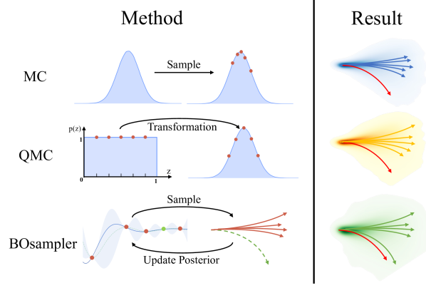
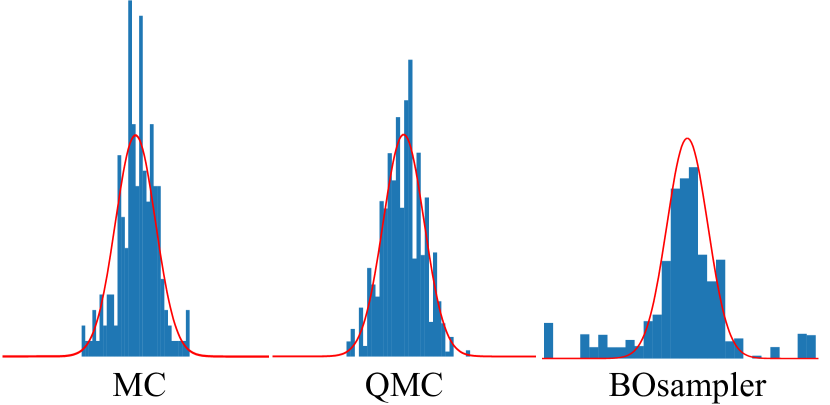
Instead of a single prediction, the inference process of these stochastic prediction methods produces a finite set of plausible future trajectories by Monte Carlo (MC) random sampling. However, the distributions are always uneven and biased, where the common choices like “go straight” are in high probability. In contrast, many other choices such as “turn left/right” and “U-turn” are in low probability. Due to the long tail effect of predicted distribution, finite samples are insufficient to cover the realistic paths. For example, as shown in Figure 1, MC sampling tends to generate redundant trajectories with high probability but ignores the potential low-probability choice. To solve this problem, some methods [31, 4] trained the model using an objective term to increase the diversity of samples, e.g., maximizing the distance among the predicted samples. Though improving the sampling diversity, these methods need to re-train the model by adding the loss term. It is timely-cost and may fail when only the model is given (the source data is inaccessible).

In this paper, we propose an unsupervised method to promote the sampling process of stochastic prediction without accessing the source data. It is named BOsampler , which refines the sampling for more exploration via Bayesian optimization (BO). Specifically, we first formulate the sampling process as a Gaussian Process (GP), where the posterior is conditioned by previous sampling trajectories. Then, we define an acquisition function to measure the value of potential samples, where the samples fitting the trained distribution well or away from existing samplings obtain high values. By this acquisition function, we can encourage the model to explore paths in the long-tail region and achieve a trade-off between accuracy and diversity. As shown in Figure 1, we compare BOsampler with MC and another sampling method QMC [4], which first generates a set of latent variables from a uniform space and then transfers it to prior distribution for trajectory sampling. Compared with them, BOsampler can adaptively update the Gaussian posterior based on existing samples, which is more flexible. We highlight that BOsampler serves as a plug-and-play module that could be integrated with existing multi-modal stochastic predictive models to promote the sampling process without retraining. In the experiments, we apply the BOsampler on many popular baseline methods, including Social GAN [18], PECNet [33], Trajectron++ [41], and Social-STGCNN [35], and evaluate them on the ETH-UCY datasets. The main contributions of this paper are summarized as follows:

• We present an unsupervised sampling prompting method for stochastic trajectory prediction, which mines potential plausible paths with Bayesian optimization adaptively and sequentially.

• The proposed method can be integrated with existing stochastic predictors without retraining.

• We evaluate the method with multiple baseline methods and show significant improvements.

2 Related Work

Trajectory Prediction with Social Interactions. The goal of human trajectory forecasting is to infer plausible future positions with the observed human paths. In addition to the destination, the pedestrian’s motion state is also influenced by the interactions with other agents, such as other pedestrians and the environment. Social-LSTM [2] apply a social pooling layer to merge the social interactions from the neighborhoods. To highlight the valuable clues from complex interaction information, the attention model is applied to mine the key neighbourhoods [13, 53, 58, 68, 1]. Besides, for the great representational ability of complex relations, some methods apply graph model to social interaction [20, 47, 7, 56, 60, 3]. To better model social interactions and temporal dependencies, different model architectures are proposed for trajectory prediction, such as RNN/LSTM [64], CNN [37, 35], and Transformer [28, 61, 52, 62]. Beyond human-human interactions, human-environment interaction is also critical to analyze human motion. To incorporate the environment knowledge, some methods encode the scene image or traffic map with the convolution neural network [55, 49, 48, 34, 69, 57].

Stochastic Trajectory Prediction. The above deterministic trajectory prediction methods only generate one possible prediction, ignoring human motion’s multimodal nature. To address this problem, stochastic prediction methods are proposed to represent the multimodality by the generative model. Social GAN [18] first introduces the Generative adversarial networks (GANs) to model the indeterminacy and predict socially plausible futures. In the following, some GAN-based methods are proposed to integrate more clues [40, 10] or design more efficient models [24, 12, 46]. Another kind of methods [21, 8, 25, 9, 59, 19, 63] formulates the trajectory prediction as CVAE [45], which applies observed trajectory as condition and learn a latent random variable to model multimodality. Besides, some methods explicitly use the endpoint [33, 65, 32, 66, 15, 14] to model the possible destinations or learn the grid-based location encoder [29, 11, 17] generate acceptable paths. Another Recently, Gu et al. [16] proposes to use the denoise diffusion probability model(DDPM) to discard the indeterminacy gradually to obtain the desired trajectory region. Beyond learning a better probability distribution of human motion, some methods [31, 4] focus on learning the sampling network to generate more diverse trajectories. However, these methods need to retrain the model, which is timely-cost and can only work when source data is given.

Bayesian Optimization. The key idea of Bayesian optimization (BO) [42] is to drive optimization decisions with an adaptive model. Fundamentally, it is a sequential model to find the global optimization result of an unknown objective function. Specifically, it initializes a prior belief for the objective function and then sequentially updates this model with the data selected by Bayesian posterior. BO has emerged as an excellent tool in a wide range of fields, such as hyper-parameters tuning [44], automatic machine learning [54, 23], and reinforcement learning [6]. Here, we introduce BO to prompt the sampling process of stochastic trajectory forecasting models. We formulate the sampling process as a sequential Gaussian process and define an acquisition function to measure the value of potential samples. With BO, we can encourage the model to explore paths in the long-tail regions.

3 Method

In this section, we will introduce our unsupervised sampling promoting method, BOsampler , which is motivated by Bayesian optimization to sequentially update the sampling model given previous samples. First, we formulate the sampling process as a Gaussian process where new samples are conditioned on previous ones. Then we show how to adaptively mine the valuable trajectories by Bayesian Optimization. Finally, we provide a detailed optimization algorithm of our method.

3.1 Problem Definition

Given observed trajectories for $L$ pedestrians with time steps t=1,…,$T_{obs}$ in a scene as $X_l^{1:T_{obs}}=\{X_l^t|t\in [1,\mathrm{\dots },T_{obs}]\}$ for $\forall l\in [1,\mathrm{\dots },L]$, the trajectory predictor will generate N possible future trajectories ${\widehat{Y}}_l^{1:T_{pred}}=\{{\widehat{Y}}_{l,n}^t|t\in [1,\mathrm{\dots },T_{pred}],n\in [1,\mathrm{\dots },N]\}$ for each pedestrian, where $X_l^t$ and $Y_l^t$ are both 2D locations. For the sake of simplicity, we remove the pedestrian index $l$ and time sequences $1:T_{obs}$ and $1:T_{pred}$ without special clarification, e.g., using $X$ and ${\widehat{Y}}_n$ to respectively represent the observed trajectory and one of the generated future paths. Then the trajectory prediction system can be formulated as:

$\widehat{Y}:=G_{\theta }(X,\text{z}),$ (1)

where $G_{\theta }$ denotes a predictor with learned parameters $\theta$ , and z is a latent variable with distribution $p_{\mathrm{z}}$ to model the multimodality of human motion. For a GAN-based model, $p_{\mathrm{z}}$ is a multivariate normal distribution, and for a CVAE-based model, $p_{\mathrm{z}}$ is a latent distribution. In the inference stage, we will sample a sequence of values of latent variable ${\{{\text{z}}_n\}}_{n=1}^N\in p_{\mathrm{z}}$ to generate a finite set of future trajectories as ${\widehat{Y}}_n:=G_{\theta }(X,{\text{z}}_n)$.

Figure 2: An illustration of how BOsampler generate new samples in an iterative manner. Given w existing samples, we first characterize two functions: ${\mu }_w$ and $\sqrt{\beta {\kappa }_w}$. Then, we use these two functions to fit a Gaussian Process and calculate the posterior distribution. Next, we use the posterior distribution to calculate the acquisition function $\varphi ({\text{z}}_w)$. Then, the next sample is generated by maximizing $\varphi ({\text{z}}_w)$. Finally, we add this new sample to inputs and can use it to update the distribution.

3.2 BOsampler

Conventional stochastic trajectory prediction methods sample latent variables in a Monte Carlo manner based on learned distribution. Despite learning well, the distributions are always uneven and biased, where the common choices like “go straight” are in high probability and other choices such as “U-turn” are in low probability. Due to this long-tail characteristic of distribution, finite trajectories with overlapped high-probability paths and less low-probability paths cannot cover the realistic distribution. Though low-probability situations are the minority in the real world, they may raise potential serious safety problems, which are important for the applications such as auto-driving.

To solve this problem, we propose to select valuable samples with Bayesian optimization. The optimization objective can be formulated as:

${\text{z}}^{\ast }=\underset{\text{z}\in 𝒵}{\arg \max }{\displaystyle \sum _{l=1}^L}D(G_{\theta }(X_l,\text{z})),$ (2)

where $G_{\theta }(X_l,\text{z})$ denotes the generated trajectory and $D$ is a metric to evaluate the quality of the sampling, e.g., the average distance error (ADE) of the trajectory. Given the sampling space, $\text{z}\in 𝒵$, the goal of BOsampler is to find a ${\text{z}}^{\ast }$ to achieve the best score of the evaluation metric using a finite number of samples. For simplicity, we define the above objective function as $f(\text{z})={\sum }_{l=1}^{L}D(G_{\theta }(X_l,\text{z}))$.

3.2.1 Gaussian Process

To optimize the $f(\text{z})$, we formulate the sampling as a sequential Gaussian process defined on the domain $𝒵$, which is characterized by a mean function $\mu (\text{z}):𝒵\to ℝ$ and a covariance function $\kappa (\text{z}):{𝒵}^2\to ℝ$ (defined by the kernel). This Gaussian process can serve as a probabilistic surrogate of the objective function as:

$f(\text{z})\sim 𝒢𝒫(\mu (\text{z}),\kappa (𝐳,{𝐳}^{\prime })),$ (3)

where

$\mu (\text{z})$ $=𝔼[f(\text{z})]$ (4)

$\kappa (𝐳,{𝐳}^{\prime })$ $=𝔼\left[{(f(\text{z})-\mu (\text{z}))}^T(f({\text{z}}^{\prime })-\mu ({\text{z}}^{\prime }))\right].$

Given the previous $w-1$ generated paths and corresponding evaluation scores ${\mathrm{\Omega }}_{w-1}={\{({\text{z}}_i,{\text{s}}_i)\}}_{i=1}^{w-1}$ , where ${\text{z}}_i\in 𝒵$ is the sample and ${\text{s}}_i=f({\text{z}}_i)+{ϵ}_i\in ℝ$ is the real evaluation score with possible measure noise $ϵ\sim 𝒩(0,{\delta }^2)$, we want to calculate the distribution of the next generated sample and score $({\text{z}}_w,f({\text{z}}_w))$. Define that the vectors $𝒔={[{\text{s}}_1,{\text{s}}_2,\mathrm{\dots },{\text{s}}_{w-1}]}^T\in {ℝ}^{w-1}$, $𝒛={[{\text{z}}_1,{\text{z}}_2,\mathrm{\dots },{\text{z}}_{w-1}]}^T\in {ℝ}^{w-1}$. Then Define that the kernel matrix $𝑲\in {ℝ}^{(w-1)\times (w-1)}$ with ${𝑲}_{i,j}=\kappa ({\text{z}}_i,{\text{z}}_j)$, and $𝒌,{𝒌}^{\prime }\in {ℝ}^{w-1}$ are two vectors from $𝑲$ as ${𝒌}_i=\kappa (\text{z},{\text{z}}_i)$ and ${𝒌}_i^{\prime }=\kappa ({\text{z}}^{\prime },{\text{z}}_i)$. The joint distribution of previous scores $𝒔$ and the next score ${\text{s}}_w$ can be formulated as:

(5)

Here, the posterior distribution $f({\text{z}}_w)|{\mathrm{\Omega }}_{w-1}\sim 𝒩({\mu }_w({\text{z}}_w),{\kappa }_w({\text{z}}_w))$ is still a Gaussian distribution by utilizing the properties of Gaussian process. The mean and covariance functions of this posterior distribution can be formulated as:

${\mu }_w({\text{z}}_w)$ $=\mu ({\text{z}}_w)+{𝒌}^T{(𝑲+{\sigma }^2𝑰)}^{-1}(𝒔-\mu (𝒛))$ (6)

${\kappa }_w({\text{z}}_w,{\text{z}}_w)$ $=\kappa ({\text{z}}_w,{\text{z}}_w)-{𝒌}^T{(𝑲+{\sigma }^2𝑰)}^{-1}{𝒌}^{\prime }.$

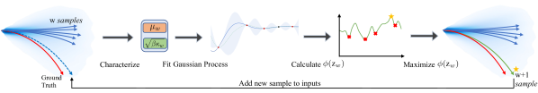
This closed-form solution of the posterior process indicates that we can easily update the probabilistic model of $f(\text{z})$ with new sample ${\text{z}}_w$. As shown in Figure 2, we can iteratively use the posterior distribution to select new samples and use new samples to update the distribution. Specifically, given the $w-1$ sampled trajectories and the corresponding latent variables, we first obtain a database ${\mathrm{\Omega }}_{w-1}={\{({\text{z}}_i,{\text{s}}_i)\}}_{i=1}^{w-1}$. Then we can calculate the posterior distribution of the possible evaluation score $f({\text{z}}_w)$, and use this posterior distribution to select the next sample ${\text{z}}_w$. Then we add this sample to the database to obtain ${\mathrm{\Omega }}_w$ and further select ${\text{z}}_{w+1}$.

3.2.2 Acquisition Function

To select the next sample, we apply this posterior distribution to define an acquisition function $\varphi (\text{z})$ to measure the value of each sample. On the one hand, the good samples deserve a high evaluation score $f(\text{z})$. On the other hand, we encourage the model to explore the regions never touched before. To achieve this goal, we define the acquisition function $\varphi (\text{z})$ as:

$\varphi ({\text{z}}_w)={\mu }_w({\text{z}}_w)+\sqrt{\beta {\kappa }_w({\text{z}}_w,{\text{z}}_w^{\prime })},$ (7)

where the first term denotes that we would like to select the samples with high score expectations, and the second term indicates to select the samples with more uncertainty (variance). Both two terms come from the posterior distribution. We use a hyper-parameter $\beta$ to balance the accuracy (high score expectation) and diversity (high uncertainty). We then maximize this acquisition function as ${\text{z}}_w^{\ast }=\arg \max \varphi ({\text{z}}_w)$ to select the next samples.

However, different from typical Bayesian Optimization, our task finds the score function inaccessible since we cannot obtain the ground-truth trajectory during sampling. To solve this problem, we propose a pseudo-score evaluation function to approximate the ground-truth function. Specifically, we assume only slight bias exists between the training and testing environment, and the same for using the most likely predicted trajectory and the pseudo ground truth. Taking the ADE as an example, we calculate the evaluation score as:

$f(\text{z})=-{\displaystyle \sum _{l=1}^L}{D}_{ade}(G_{\theta }(X,\text{z}),G_{\theta }(X,\tilde{\text{z}})),$ (8)

where $\tilde{\text{z}}=\arg \max p_{\mathrm{z}}$ denotes the most-likely prediction. It means that we trust the trained model without any information update.

Table 1: Quantitative results on the exception subset with Best-of-20 strategy in ADE/FDE metric. We select the abnormal trajectories from ETH-UCY to benchmark the sampling methods for abnormal situations such as turning left/right or U-turn, which is important for safety. Gain: the average performance improvement of ADE and FDE to MC, higher is better.

Baseline Model	Sampling	ETH		HOTEL		UNIV		ZARA1		ZARA2		AVG		Gain
		ADE	FDE	ADE	FDE	ADE	FDE	ADE	FDE	ADE	FDE	ADE	FDE	ADE	FDE
Social-GAN [18]	MC	1.52	2.37	0.61	1.21	0.91	1.86	0.78	1.63	0.90	1.97	0.94	1.80	/	/
	QMC	1.56	2.74	0.60	1.12	0.91	1.85	0.77	1.60	0.92	2.00	0.95	1.86	-1%	-3%
	BOSampler	1.14	2.04	0.52	1.03	0.80	1.62	0.68	1.41	0.75	1.60	0.78	1.54	18%	15%
Trajectron++ [41]	MC	0.59	1.41	0.20	0.44	0.37	0.87	0.15	0.35	0.22	0.47	0.30	0.71	/	/
	QMC	0.61	1.45	0.20	0.43	0.36	0.86	0.15	0.35	0.22	0.48	0.31	0.71	-1%	-1%
	BOSampler	0.52	0.95	0.19	0.39	0.30	0.67	0.14	0.33	0.20	0.45	0.27	0.56	11%	21%
PECNet [33]	MC	2.80	5.38	0.59	0.94	1.14	2.04	0.76	1.52	0.76	1.51	1.21	2.33	/	/
	QMC	2.81	5.35	0.59	0.98	1.13	2.28	0.68	1.36	0.78	1.56	1.20	2.31	1%	1%
	BOSampler	2.11	3.73	0.46	0.72	0.97	1.87	0.66	1.27	0.65	1.18	0.97	1.75	19%	25%
Social-STGCNN [35]	MC	2.18	4.14	0.30	0.51	0.57	1.05	0.56	1.03	0.50	0.96	0.82	1.54	/	/
	QMC	2.20	3.66	0.26	0.42	0.45	0.80	0.48	0.86	0.44	0.79	0.77	1.31	7%	15%
	BOSampler	0.87	1.13	0.18	0.32	0.58	1.06	0.52	0.96	0.45	0.86	0.52	0.87	37%	44%
STGAT [20]	MC	1.73	3.49	0.60	1.10	0.92	1.94	0.69	1.41	0.90	1.87	0.97	1.96	/	/
	QMC	1.80	3.61	0.56	0.98	0.89	1.87	0.67	1.33	0.88	1.85	0.96	1.93	1%	2%
	BOSampler	0.97	1.57	0.56	1.01	0.83	1.74	0.63	1.23	0.83	1.71	0.76	1.45	21%	26%

3.3 Technical Details

To optimize the sampling process smoothly, we apply some technical tricks for our BOsampler .

Warm-up. First, we use a warm starting to build the Gaussian process. It randomly samples w latent variables and generates trajectories to obtain the first understanding of $f(\text{z})$ as prior. This warm stage is the same as the original MC random sampling. We choose the number of warm-ups as half of the total number of sampling in our experiments. In Sec. 4.4, we provide quantitative analysis about the number of warm-ups

Acquisition Function. For the acquisition function, we set the latent vector $z$ to a zero vector to generate the pseudo label, and use the pseudo label to obtain the pseudo-score as equation 8. Then we tune the hyper-parameter $\beta$ of the acquisition function between $[0.1,1]$ because it’s within the commonly used range in applications of Bayesian Optimization. Please refer to Eq. 8 for details.

Calculation. To make BOsampler computes on GPU as the same as the pre-trained neural networks, we use BoTorch[5] as our base implementation. Also, we modify some parts related to the acquisition function and batch computation accordingly.

Overall, BOsampler is an iterative sampling method. Given a set of samples, we first build the Gaussian process and obtain the posterior distribution as equation 6. Then, we calculate the acquisition function as equation 7 and generate the new sample with the latent variable ${\text{z}}^{\ast }$ with the highest acquisition value. Finally, we add the new sample into the database and repeat this loop until we get enough samples.

4 Experiments

In this section, we first quantitatively compare the performance of our BOsampler with other sampling methods using five popular methods as baselines on full ETH-UCY dataset and the hard subset of it. Then, qualitatively, we visualize the sampled trajectories and their distribution. Finally, we provide an ablation study and parameters analysis to further investigate our method.

4.1 Experimental Setup

Dataset. We evaluated our method on one of the most widely used public human trajectory prediction benchmark dataset: ETH-UCY [38, 27]. ETH-UCY is a combination of two datasets with totally five different scenes, where the ETH dataset [38] contains two scenes, ETH and HOTEL, with 750 pedestrians, and the UCY dataset [27] consists of three scenes with 786 pedestrians including UNIV, ZARA1, and ZARA2. All scenes are captured in unconstrained environments such as the road, cross-road, and almost open area. In each scene, the pedestrian trajectories are provided in a sequence of world-coordinate. The data split of ETH-UCY follows the protocols in Social-GAN and Trajectron++ [18, 41]. The trajectories are sampled at 0.4 seconds interval, where the first 3.2 seconds (8 frames) is used as observed data to predict the next 4.8 seconds (12 frames) future trajectory.

To evaluate the performance on the uncommon trajectories (e.g. the pedestrian suddenly makes a U-turn right after the observation), we select a exception subset consisting of the most uncommon trajectories selected from ETH/UCY. To quantify the rate of exception, we use a linear method [22], an off-the-shelf Kalman filter, to give a reference trajectory. Since it is a linear model, the predictions can be regarded as normal predictions. Then we calculate FDE between the ground truth and reference trajectory as a metric of deviation. If the derivation is relatively high, it means that the pedestrian makes a sudden move or sharp turn afterward. Finally, we select the top 4% most deviated trajectories from each dataset of UCY/ETH as the exception subset.

Table 2: Quantitative results on the ETH/UCY dataset with Best-of-20 strategy in ADE/FDE metric. Lower is better. * updated version of Trajectron++

Baseline Model	Sampling	AVG
		ADE	FDE
Social-GAN [18]	MC	0.53	1.05
	QMC	0.53	1.03
	BOSampler	0.52	1.01
	BOSampler + QMC	0.52	1.00
Trajectron++ [41]	MC	0.21	0.41
	QMC	0.21	0.40
	BOSampler	0.18	0.36
	BOSampler + QMC	0.18	0.36
Trajectron++ [41] *	MC	0.28	0.54
	QMC	0.28	0.54
	BOSampler	0.25	0.45
	BOSampler + QMC	0.25	0.45
PECNet [33]	MC	0.32	0.56
	QMC	0.31	0.54
	BOSampler	0.30	0.51
	BOSampler + QMC	0.30	0.50
Social-STGCNN [35]	MC	0.45	0.75
	QMC	0.39	0.65
	BOSampler	0.41	0.69
	BOSampler + QMC	0.37	0.62
STGAT [20]	MC	0.46	0.90
	QMC	0.45	0.89
	BOSampler	0.44	0.85
	BOSampler + QMC	0.44	0.84

Evaluation Metric. We follow the same evaluation metrics adopted by previous stochastic trajectory prediction methods [18, 33, 43, 20, 16], which use widely-used evaluation metrics: minimal Average Displacement Error (minADE) and minimal Final Displacement Error (minFDE). ADE denotes the average error between all the ground truth positions and the estimated positions while FDE computes the displacement between the endpoints. Since the stochastic prediction model generates a finite set ($N$) of trajectories instead of the single one, we use the minimal ADE and FDE of $N=20$ trajectories following [18, 41], called Best-of-20 strategy. For the ETH-UCY dataset, we use the leave-one-out cross-validation evaluation strategy where four scenes are used for training and the remaining one is used for testing. Besides, for all experiments, we evaluate methods 10 times and report the average performance for robust evaluation.

Baseline Methods. We evaluate our BOsampler with five mainstream stochastic pedestrian trajectory prediction methods, including Social-GAN [18], PECNet [33], Trajectron++ [41], Social-STGCNN [35] and STGAT [20]. Social-GAN [18] learns a GAN model with a normal Gaussian noise input to represent human multi-modality. BOsampler optimizes the sampled noise to encourage diversity. STGAT [20] is an improved version of Social-GAN, which also learns a GAN model for motion multi-modality and applies the graph attention mechanism to encode spatial interactions. PECNet [33] applies the different endpoints to generate multiple trajectories. We optimize these end-points whose prior is the learned Endpoint VAE. Trajectron++ [41] uses the observation as the condition to learn a CVAE with the learned discrete latent variable. Social-STGCNN [35] directly learns parameters of the Gaussian distribution of each point and samples from it. Here, we can directly optimize the position of points. All these baseline methods use the Monte Carlo (MC) sampling methods for generations. We can directly change the sampling manner from MC to our BOsampler with their trained models, i.e. our method doesn’t need any training data to refine the sampling process. Beyond MC sampling, we also compare BOsampler with Quasi-Monte Carlo (QMC) sampling introduced in [4], which uses low-discrepancy quasi-random sequences to replace the random sampling. It can generate evenly distributed points and achieve more uniform sampling.

Figure 3: Visualization of trajectories with sample number $N=4,8,12,16,20$, generated by MC, QMC and BOsampler . Different from MC and QMC whose sampling distribution is the same with all sample numbers, BOsampler adaptively modifies the sampling distribution with existing samples.

4.2 Quantitative Comparison

Performance on the exception subset of ETH-UCY. The goal of our method is to help models to generate more comprehensive and reliable samples. Thus, we focus on abnormal situations such as turning left, turning right, or U-turn. Though these situations are the minority of all trajectories, they are still crucial for the applications such as intelligent transportation and auto-driving due to their safety and reliability. The detailed selection procedure of the exception subset is explained in Sec. 4.1. As shown in Tab. 1, we give minADE and minFDE results using the same pre-trained model across different sampling methods including MC, QMC, and BOsampler , based on five baseline methods. BOsampler shows a significant improvement in exception trajectories compared to MC and QMC. The average performance gain rate of BOsampler to MC on ADE/FDE among five baseline models is 23.71% and 27.49%, respectively. It implies that the promotion of BOsampler over the original fixed pre-trained model mainly lies in the rare trajectories.

Performance on ETH-UCY. Beyond the exceptional cases, we also quantitatively compare BOsampler with MC and QMC sampling methods on the original ETH-UCY dataset. As shown in Tab. 2, we provide the minADE and minFDE results using the same pre-trained model and different sampling methods. Here, we only report the average results on all five scenes. Please kindly refer to the supplementary materials for the complete experimental results on each scene. For all baseline methods, BOsampler consistently outperforms the MC sampling method, which shows the effectiveness of the proposed method, though not much. It is reasonable that all results from a fixed model with different sampling methods are comparable because only a small part of trajectories are uncommon (lie in low probability), while most testing trajectories are normal. But we want to highlight that these low-probability trajectories may raise safety risks for autonomous driving systems. The results show that BOsampler can provide a better prediction for possible low-probability situations without reducing the accuracy of most normal trajectories. In addition, BOsampler also shows an improvement over the QMC method on most baselines. For Social-STGCNN [35], though BOsampler achieves improvement over the MC method by a more considerable margin, it is still slightly lower than the QMC method. It is because Social-STGCNN adds the indeterminacy on each position, whose variable dimension is too large ($2\times 12=24$) for Bayesian Optimization. Furthermore, we also show that the proposed BOsampler is not contradictory to the QMC method. Using QMC in the warm-up stage, we can further improve the performance of BOsampler . For example, for Social-STGCNN, BOsampler + QMC can further improve the QMC method and achieve 0.37 ADE and 0.62 FDE. Please note that we don’t compare with the NPSN method [4] since it is a supervised method that needs to access the source data and re-train the models.

4.3 Qualitative Comparison

We further investigate our method with three qualitative experiments. Firstly, we visualize the sampled trajectories of MC, QMC, and BOsampler with different sample numbers. Secondly, we visualize and compare the best predictions among sampled trajectories of MC, QMC, and BOsampler in the real environment. Thirdly, we also provide the visualization of some failure cases.

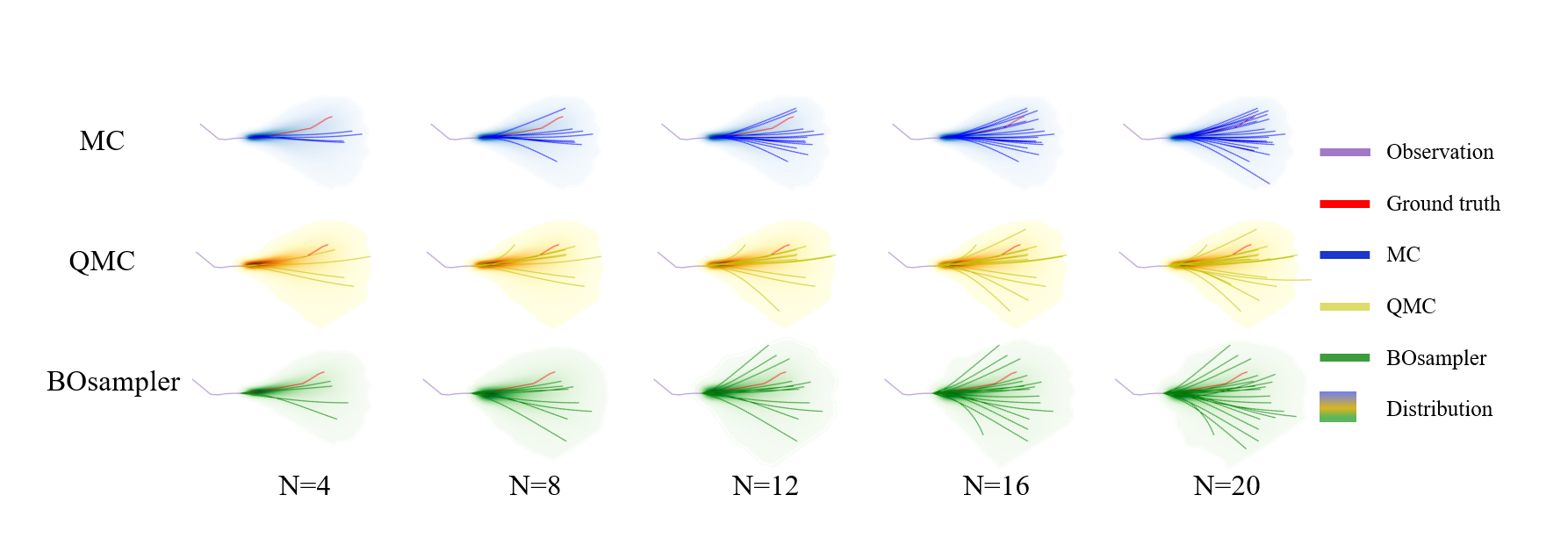
Trajectories with different sample numbers. In this experiment, we aim to investigate how the sampling (posterior) distribution changes with the increase of the sampling number. As shown in Figure 3, we provide the sampling results of MC, QMC, and BOsampler with sample number $N=4,8,12,16,20$, where the light area denotes the sampling (posterior) distribution. We can observe that the sampling distributions of both MC and QMC are unchanged. The only difference is that QMC smooths the original distribution. It indicates that QMC may not work well when the sampling number is small since the distribution is changed suddenly. Unlike them, BOsampler gradually explore the samples with low probability with the increase of the sample number, which can achieve an adaptive balance between diversity and accuracy. When the sampling number $N$ is small, BOsampler tends to sample close to the prior distribution. When $N$ is larger, the model is encouraged to select those low-probability samples.

Figure 4: Visualization of our method in five datasets. We sampled 20 times with MC, QMC, and BOsampler and compared the best-predicted trajectories from the sampled results. And the light areas are density graphed generated by sampling 2000 times with MC.

Figure 5: Frequency histogram of MC, QMC, and BOsampler

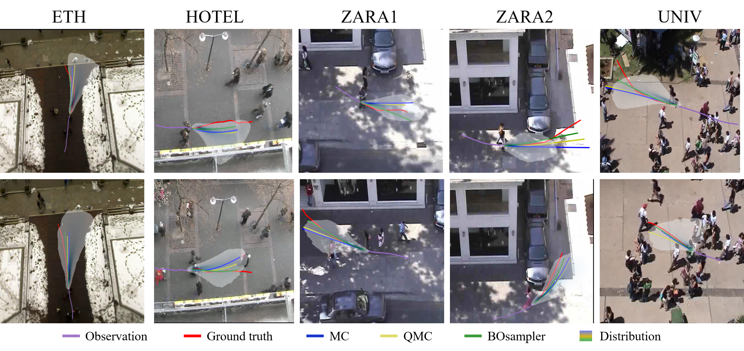
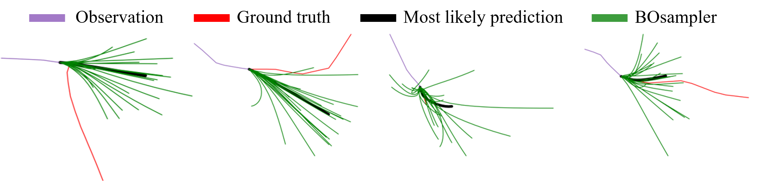
Visualization. We also compare the best predictions of different sampling methods to provide an intuition in which situation BOsampler works well. As shown in Figure 4, we give the best predictions of different sampling methods and the ground truth trajectory on five scenes in the ETH-UCY dataset. We observe that BOsampler can provide the socially-acceptable paths in the low-probabilities (away from normal ones). For example, when the pedestrian turns left or right, the gourd truth will be far away from the sampled results of MC and QMC, but our method’s sampled results are usually able to cover this case. It indicates that BOsampler encourage the model to explore the low-probability choices. Besides, we also provide the visualization of the failure cases to understand the method better. We found that BOsampler may lose the ground truth trajectory when the most-likely prediction is far away from the ground truth.

Besides, as shown in Figure 5, we visualize the optimized sampling distributions of MC, QMC, and BOsampler with the original standard Gaussian distribution $𝒩(0,1)$. By the simulation results, we show that BOsampler can mitigate the long-tail property, while MC and QMC cannot.

Figure 6: Left: ADE and FDE with different warm-up samples by BOsampler on PECNet.
Right: ADE and FDE with different hyper-parameters $\beta$ by BOsampler on PECNet.

4.4 Ablation Studies and Parameters Analysis

In this subsection, we conduct ablation studies and parameters analysis to investigate the robustness of different hyper-parameters. Then, we provided a detailed analysis of the sampling process with a different number of samples.

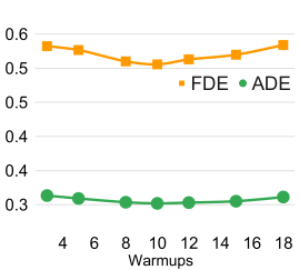
Analysis with warm-up: We choose among the number of warm-up $\text{w}=3,5,8,10,12,15,18$, and then we use PECNet as the baseline model. The results on the ETH/UCY dataset with the Best-of-20 strategy are shown in the top row of Figure 6. For all the numbers of warm-ups, BOsampler achieves better performance than the MC baseline. When the number of warm-ups is close to half of the number of samples, which is 10, the corresponding ADE/FDE is better than other options. Although decreasing the number of warm-ups will encourage more exploration by increasing the number of BOsampler , the performance overall will be hurt because the abnormal trajectories only make up a relatively small portion of the entire dataset. Setting the number of warm-up to half of the number of entire samples helps balance exploration and exploitation.

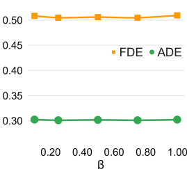
Analysis with acquisition function: We analyze the robustness of the hyper-parameter by selecting $\beta \in [0.1,1]$, separated evenly in this range. We choose PECNet as a base model and use the Best-of-20 strategy to evaluate on the ETH/UCY dataset. The performance is close among five acquisition factors $\beta$, which means the performance of BOsampler is stable when the acquisition factor is set within a reasonable range.

(a) Social GAN

(b) PECNet

Figure 7: ADE, FDE, and performance gain of BOsampler to MC on Social GAN and PECNet across a different number of samples.

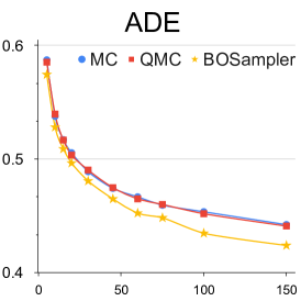
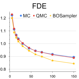
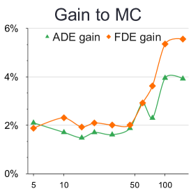
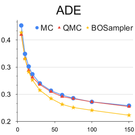
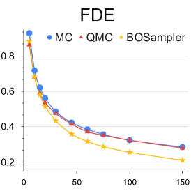
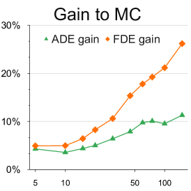
Analysis with different number of samples: We provide this quantitative experiment with respect to the number of samples to better understand the simpling process of our BOsampler . As shown in Figure 7, we compare the ADE and FDE on the ETH-UCY dataset of MC, QMC, and BOsampler with different numbers of samples on Social GAN and PECNet. We choose a number of samples $N=5,10,15,20,30,45,60,75,100,150$. BOsampler works well in all settings, which demonstrates an adaptive balance between diversity and accuracy. It also shows that BOsampler will work even if the warm-up steps are extremely small (less than five as is shown in this case). Besides, we find that our BOsampler obtains a larger improvement over MC than the improvement of QMC when the number of samples increases. With the Gaussian process, BOsampler can gradually refine the posterior distribution with the sampling process.

5 Conclusion

In this paper, we have proposed an unsupervised sampling method, called BOsampler, to promote the sampling process of the stochastic trajectory prediction system. In this method, we formulate the sampling as a sequential Gaussian process, where the current prediction is conditioned on previous samples. Using Bayesian optimization, we defined an acquisition function to explore potential paths with low probability adaptively. Experimental results demonstrate the superiority of BOsampler over other sampling methods such as MC and QMC.

Broader Impact & limitations: BOsampler can be integrated with existing stochastic trajectory prediction models without retraining. It provides reasonable and diverse trajectory sampling, which can help the safety and reliability of intelligent transportation and autonomous driving. Despite being training-free, this inference time sampling promoting method still requires a time cost due to sequential modeling. Taking Social GAN as a baseline, our method needs $8.56s$ for predicting 512 trajectories while MC needs $4.92s$. Better computational techniques may mitigate this issue.

Appendix for BoSampler

Appendix A The algorithm of BOsampler

We give the algorithm to give a short but clear summarization of BOsampler . The detailed algorithm is shown in Algorithm 1.

Algorithm 1 Sampling procedure of BOsampler

generator G, observed trajectory $X$, pseudo score evaluation function f.

for $n$ in {1,…,w} do $▷$ Warm-up

Sample ${\text{z}}_n\sim p_{\text{z}}$

${\widehat{Y}}_n\leftarrow G(X,{\text{z}}_n)$

end for

for $n$ in {w+1,…,N} do $▷$ BOsampler

Fit the Gaussian Process $𝒢𝒫$ by ${\text{z}}_{1:n-1}$ and $f({\text{z}}_{1:n-1})$

Use the posterior of $𝒢𝒫$ to build the acquisition function ${\varphi }_n(\text{z})$

${\text{z}}_n\leftarrow \underset{\text{z}}{\mathrm{argmax}}{\varphi }_n(\text{z})$

${\widehat{Y}}_n\leftarrow G(X,{\text{z}}_n)$

end for

Return $\widehat{Y}=\{{\widehat{Y}}_n|n\in [1,\mathrm{\dots },N]\}$

Appendix B Complete quantitative experimental results on ETH/UCY

We present the complete experiment results on five scenes of ETH/UCY datasets in Tab. 4. For all baseline methods, BOsampler consistently outperforms the MC sampling method, which shows the effectiveness of the proposed method, though not much. BOsampler also shows an improvement over the QMC method on most baselines. BOsampler doesn’t have the same level of performance gain in the complete set of ETH/UCY compared to the exception subset. It is because the uncommon trajectories only comprise a small portion of the dataset. BOsampler achieves more performance gain on the ETH dataset. The reason is probably the same: uncommon trajectories show up more frequently in ETH dataset than in the other four datasets in ETH/UCY. Although BOsampler does not achieve a huge improvement in the complete set, considering BOsampler has a significant gain in the exception subset, it is clear that BOsampler balances exploitation of the baseline model’s distribution and exploration of the edge cases. So BOsampler helps promote the robustness of the sampling process of baseline models. We highlight that BOsampler focus on trajectories with low probability. Although these cases are the minority, it is meaningful and crucial to consider them in intelligent transportation and autonomous driving.

Figure 8: Failure cases: In the first and second graph, we show that when a pedestrian changes direction suddenly, our method may not predict such a change. In the third graph, when a pedestrian stops suddenly (e.g. a pram gets stuck in the ground), or when a pedestrian suddenly starts walking, our method may also fail.

	top 4%	top 12%	full
MC	1.21/2.33	0.88/1.76	0.32/0.56
QMC	1.20/2.33	0.86/1.70	0.31/0.54
BOsampler	0.97/1.75	0.74/1.38	0.30/0.51

Table 3: The results of PECNet on ETH-UCY with different exception ratios.

Appendix C Experiments on exception subsets with different ratios

In Section 4.2 of the main manuscript, we set the ratio of the exception set as 4%. In order to verify the validity of the chosen subset, we further provide a 12% variation, which demonstrates a consistent performance trend with the original subset, thus confirming the representativeness and appropriateness of the ratio setting of our experiments. The experiment results are presented in Tab. 3. When the ratio goes to 12%, BOsampler still achieves considerably better performance than baselines.

Appendix D Visualization of the failure cases

We provide the visualization of the failure cases to better understand the method. From the visualization in Fig. 8, we found BOsampler may lose the ground truth trajectory when the most-likely prediction is far away from the ground truth. It is not surprising since our method is based on the assumption of the good prior distribution. Solving this problem without accessing more data is not trivial. A potential solution is to modify the prior distribution using the testing data during the inference [50].

Table 4: Quantitative results on the ETH/UCY dataset with Best-of-20 strategy in ADE/FDE metric. Lower is better. * updated version of Trajectron++

Baseline Model	Sampling	ETH		HOTEL		UNIV		ZARA1		ZARA2		AVG
		ADE	FDE	ADE	FDE	ADE	FDE	ADE	FDE	ADE	FDE	ADE	FDE
Social-GAN [18]	MC	0.77	1.40	0.43	0.88	0.75	1.50	0.35	0.69	0.36	0.72	0.53	1.05
	QMC	0.76	1.38	0.43	0.87	0.75	1.50	0.34	0.69	0.35	0.72	0.53	1.03
	BOSampler	0.73	1.28	0.43	0.87	0.75	1.50	0.34	0.69	0.35	0.71	0.52	1.01
	BOSampler + QMC	0.72	1.26	0.43	0.87	0.74	1.49	0.34	0.69	0.35	0.71	0.52	1.00
Trajectron++ [41]	MC	0.43	0.86	0.12	0.19	0.22	0.43	0.17	0.32	0.12	0.25	0.21	0.41
	QMC	0.43	0.84	0.12	0.19	0.22	0.42	0.17	0.31	0.12	0.24	0.21	0.40
	BOSampler	0.34	0.64	0.12	0.21	0.18	0.40	0.14	0.30	0.11	0.24	0.18	0.36
	BOSampler + QMC	0.34	0.64	0.12	0.21	0.18	0.40	0.14	0.30	0.11	0.24	0.18	0.36
Trajectron++ [41]*	MC	0.57	1.06	0.16	0.26	0.30	0.61	0.22	0.42	0.16	0.33	0.28	0.54
	QMC	0.57	1.05	0.16	0.26	0.30	0.61	0.22	0.42	0.16	0.33	0.28	0.54
	BOSampler	0.49	0.82	0.15	0.23	0.27	0.53	0.20	0.38	0.15	0.29	0.25	0.45
	BOSampler + QMC	0.49	0.82	0.15	0.23	0.27	0.53	0.20	0.38	0.15	0.29	0.25	0.45
PECNet [33]	MC	0.61	1.07	0.22	0.39	0.34	0.56	0.25	0.45	0.19	0.33	0.32	0.56
	QMC	0.60	1.04	0.21	0.38	0.33	0.53	0.24	0.43	0.18	0.31	0.31	0.54
	BOSampler	0.56	0.92	0.21	0.38	0.32	0.52	0.24	0.42	0.18	0.31	0.30	0.51
	BOSampler + QMC	0.56	0.91	0.21	0.37	0.31	0.51	0.24	0.41	0.18	0.31	0.30	0.50
Social-STGCNN [35]	MC	0.65	1.10	0.50	0.86	0.44	0.80	0.34	0.53	0.31	0.48	0.45	0.75
	QMC	0.62	1.03	0.38	0.57	0.36	0.63	0.32	0.52	0.29	0.50	0.39	0.65
	BOSampler	0.57	0.90	0.44	0.82	0.43	0.76	0.34	0.54	0.26	0.45	0.41	0.69
	BOSampler + QMC	0.49	0.74	0.39	0.73	0.41	0.72	0.32	0.52	0.26	0.40	0.37	0.62
STGAT [20]	MC	0.74	1.34	0.35	0.68	0.56	1.20	0.34	0.68	0.29	0.59	0.46	0.90
	QMC	0.73	1.32	0.35	0.67	0.56	1.20	0.34	0.68	0.29	0.59	0.45	0.89
	BOSampler	0.70	1.15	0.35	0.67	0.55	1.17	0.34	0.68	0.29	0.59	0.44	0.85
	BOSampler + QMC	0.68	1.11	0.35	0.67	0.55	1.17	0.33	0.67	0.30	0.59	0.44	0.84

References

- [1] Vida Adeli, Mahsa Ehsanpour, Ian Reid, Juan Carlos Niebles, Silvio Savarese, Ehsan Adeli, and Hamid Rezatofighi. Tripod: Human trajectory and pose dynamics forecasting in the wild. In ICCV, pages 13390–13400, 2021.
- [2] Alexandre Alahi, Kratarth Goel, Vignesh Ramanathan, Alexandre Robicquet, Li Fei-Fei, and Silvio Savarese. Social lstm: Human trajectory prediction in crowded spaces. In CVPR, pages 961–971, 2016.
- [3] Inhwan Bae, Jin-Hwi Park, and Hae-Gon Jeon. Learning pedestrian group representations for multi-modal trajectory prediction. In ECCV, pages 270–289, 2022.
- [4] Inhwan Bae, Jin-Hwi Park, and Hae-Gon Jeon. Non-probability sampling network for stochastic human trajectory prediction. In CVPR, pages 6477–6487, 2022.
- [5] Maximilian Balandat, Brian Karrer, Daniel R. Jiang, Samuel Daulton, Benjamin Letham, Andrew Gordon Wilson, and Eytan Bakshy. BoTorch: A Framework for Efficient Monte-Carlo Bayesian Optimization. In Advances in Neural Information Processing Systems 33, 2020.
- [6] Eric Brochu, Vlad M Cora, and Nando De Freitas. A tutorial on bayesian optimization of expensive cost functions, with application to active user modeling and hierarchical reinforcement learning. arXiv preprint arXiv:1012.2599, 2010.
- [7] Guangyi Chen, Junlong Li, Jiwen Lu, and Jie Zhou. Human trajectory prediction via counterfactual analysis. In ICCV, pages 9824–9833, 2021.
- [8] Guangyi Chen, Junlong Li, Nuoxing Zhou, Liangliang Ren, and Jiwen Lu. Personalized trajectory prediction via distribution discrimination. In ICCV, pages 15580–15589, 2021.
- [9] Yuxiao Chen, Boris Ivanovic, and Marco Pavone. Scept: Scene-consistent, policy-based trajectory predictions for planning. In CVPR, pages 17103–17112, 2022.
- [10] Patrick Dendorfer, Sven Elflein, and Laura Leal-Taixé. Mg-gan: A multi-generator model preventing out-of-distribution samples in pedestrian trajectory prediction. In ICCV, pages 13158–13167, 2021.
- [11] Nachiket Deo and Mohan M Trivedi. Trajectory forecasts in unknown environments conditioned on grid-based plans. arXiv preprint arXiv:2001.00735, 2020.
- [12] Liangji Fang, Qinhong Jiang, Jianping Shi, and Bolei Zhou. Tpnet: Trajectory proposal network for motion prediction. In CVPR, 2020.
- [13] Tharindu Fernando, Simon Denman, Sridha Sridharan, and Clinton Fookes. Soft+ hardwired attention: An lstm framework for human trajectory prediction and abnormal event detection. Neural Networks, 108:466–478, 2018.
- [14] Harshayu Girase, Haiming Gang, Srikanth Malla, Jiachen Li, Akira Kanehara, Karttikeya Mangalam, and Chiho Choi. Loki: Long term and key intentions for trajectory prediction. In ICCV, pages 9803–9812, 2021.
- [15] Junru Gu, Chen Sun, and Hang Zhao. Densetnt: End-to-end trajectory prediction from dense goal sets. In ICCV, pages 15303–15312, 2021.
- [16] Tianpei Gu, Guangyi Chen, Junlong Li, Chunze Lin, Yongming Rao, Jie Zhou, and Jiwen Lu. Stochastic trajectory prediction via motion indeterminacy diffusion. In CVPR, pages 17113–17122, 2022.
- [17] Ke Guo, Wenxi Liu, and Jia Pan. End-to-end trajectory distribution prediction based on occupancy grid maps. In CVPR, pages 2242–2251, 2022.
- [18] Agrim Gupta, Justin Johnson, Li Fei-Fei, Silvio Savarese, and Alexandre Alahi. Social gan: Socially acceptable trajectories with generative adversarial networks. In CVPR, pages 2255–2264, 2018.
- [19] Marah Halawa, Olaf Hellwich, and Pia Bideau. Action-based contrastive learning for trajectory prediction. In ECCV, pages 143–159, 2022.
- [20] Yingfan Huang, HuiKun Bi, Zhaoxin Li, Tianlu Mao, and Zhaoqi Wang. Stgat: Modeling spatial-temporal interactions for human trajectory prediction. In ICCV, pages 6272–6281, 2019.
- [21] Boris Ivanovic and Marco Pavone. The trajectron: Probabilistic multi-agent trajectory modeling with dynamic spatiotemporal graphs. In ICCV, pages 2375–2384, 2019.
- [22] Rudolph Emil Kalman. A new approach to linear filtering and prediction problems. 1960.
- [23] Kirthevasan Kandasamy, Willie Neiswanger, Jeff Schneider, Barnabas Poczos, and Eric P Xing. Neural architecture search with bayesian optimisation and optimal transport. NeurIPS, 31, 2018.
- [24] Vineet Kosaraju, Amir Sadeghian, Roberto Martín-Martín, Ian Reid, Hamid Rezatofighi, and Silvio Savarese. Social-bigat: Multimodal trajectory forecasting using bicycle-gan and graph attention networks. In NeurIPS, pages 137–146, 2019.
- [25] Mihee Lee, Samuel S Sohn, Seonghyeon Moon, Sejong Yoon, Mubbasir Kapadia, and Vladimir Pavlovic. Muse-vae: Multi-scale vae for environment-aware long term trajectory prediction. In CVPR, pages 2221–2230, 2022.
- [26] Namhoon Lee, Wongun Choi, Paul Vernaza, Christopher B Choy, Philip HS Torr, and Manmohan Chandraker. Desire: Distant future prediction in dynamic scenes with interacting agents. In CVPR, pages 336–345, 2017.
- [27] Alon Lerner, Yiorgos Chrysanthou, and Dani Lischinski. Crowds by example. In Computer Graphics Forum, volume 26, pages 655–664, 2007.
- [28] Lihuan Li, Maurice Pagnucco, and Yang Song. Graph-based spatial transformer with memory replay for multi-future pedestrian trajectory prediction. In CVPR, pages 2231–2241, 2022.
- [29] Junwei Liang, Lu Jiang, Kevin Murphy, Ting Yu, and Alexander Hauptmann. The garden of forking paths: Towards multi-future trajectory prediction. In CVPR, pages 10508–10518, 2020.
- [30] Yuejiang Liu, Qi Yan, and Alexandre Alahi. Social nce: Contrastive learning of socially-aware motion representations. In ICCV, pages 15118–15129, 2021.
- [31] Yecheng Jason Ma, Jeevana Priya Inala, Dinesh Jayaraman, and Osbert Bastani. Likelihood-based diverse sampling for trajectory forecasting. In ICCV, pages 13279–13288, 2021.
- [32] Karttikeya Mangalam, Yang An, Harshayu Girase, and Jitendra Malik. From goals, waypoints & paths to long term human trajectory forecasting. In ICCV, pages 15233–15242, 2021.
- [33] Karttikeya Mangalam, Harshayu Girase, Shreyas Agarwal, Kuan-Hui Lee, Ehsan Adeli, Jitendra Malik, and Adrien Gaidon. It is not the journey but the destination: Endpoint conditioned trajectory prediction. In ECCV, 2020.
- [34] Mancheng Meng, Ziyan Wu, Terrence Chen, Xiran Cai, Xiang Sean Zhou, Fan Yang, and Dinggang Shen. Forecasting human trajectory from scene history. NeurIPS, 2022.
- [35] Abduallah Mohamed, Kun Qian, Mohamed Elhoseiny, and Christian Claudel. Social-stgcnn: A social spatio-temporal graph convolutional neural network for human trajectory prediction. In CVPR, 2020.
- [36] Harald Niederreiter. Random number generation and quasi-Monte Carlo methods. SIAM, 1992.
- [37] Nishant Nikhil and Brendan Tran Morris. Convolutional neural network for trajectory prediction. In ECCVW, pages 0–0, 2018.
- [38] Stefano Pellegrini, Andreas Ess, and Luc Van Gool. Improving data association by joint modeling of pedestrian trajectories and groupings. In ECCV, pages 452–465, 2010.
- [39] Nicholas Rhinehart, Kris M Kitani, and Paul Vernaza. R2p2: A reparameterized pushforward policy for diverse, precise generative path forecasting. In ECCV, pages 772–788, 2018.
- [40] Amir Sadeghian, Vineet Kosaraju, Ali Sadeghian, Noriaki Hirose, Hamid Rezatofighi, and Silvio Savarese. Sophie: An attentive gan for predicting paths compliant to social and physical constraints. In CVPR, pages 1349–1358, 2019.
- [41] Tim Salzmann, Boris Ivanovic, Punarjay Chakravarty, and Marco Pavone. Trajectron++: Dynamically-feasible trajectory forecasting with heterogeneous data. In ECCV, 2020.
- [42] Bobak Shahriari, Kevin Swersky, Ziyu Wang, Ryan P Adams, and Nando De Freitas. Taking the human out of the loop: A review of bayesian optimization. Proceedings of the IEEE, 104(1):148–175, 2015.
- [43] Liushuai Shi, Le Wang, Chengjiang Long, Sanping Zhou, Mo Zhou, Zhenxing Niu, and Gang Hua. Sgcn: Sparse graph convolution network for pedestrian trajectory prediction. In CVPR, pages 8994–9003, 2021.
- [44] Jasper Snoek, Hugo Larochelle, and Ryan P Adams. Practical bayesian optimization of machine learning algorithms. NeurIPS, 25, 2012.
- [45] Kihyuk Sohn, Honglak Lee, and Xinchen Yan. Learning structured output representation using deep conditional generative models. In NeurIPS, pages 3483–3491, 2015.
- [46] Hao Sun, Zhiqun Zhao, and Zhihai He. Reciprocal learning networks for human trajectory prediction. In CVPR, 2020.
- [47] Jianhua Sun, Qinhong Jiang, and Cewu Lu. Recursive social behavior graph for trajectory prediction. In CVPR, June 2020.
- [48] Jianhua Sun, Yuxuan Li, Liang Chai, Hao-Shu Fang, Yong-Lu Li, and Cewu Lu. Human trajectory prediction with momentary observation. In CVPR, pages 6467–6476, 2022.
- [49] Qiao Sun, Xin Huang, Junru Gu, Brian C Williams, and Hang Zhao. M2i: From factored marginal trajectory prediction to interactive prediction. In CVPR, pages 6543–6552, 2022.
- [50] Yu Sun, Xiaolong Wang, Zhuang Liu, John Miller, Alexei Efros, and Moritz Hardt. Test-time training with self-supervision for generalization under distribution shifts. In ICML, pages 9229–9248, 2020.
- [51] Charlie Tang and Russ R Salakhutdinov. Multiple futures prediction. In NeurIPS, pages 15398–15408, 2019.
- [52] Li-Wu Tsao, Yan-Kai Wang, Hao-Siang Lin, Hong-Han Shuai, Lai-Kuan Wong, and Wen-Huang Cheng. Social-ssl: Self-supervised cross-sequence representation learning based on transformers for multi-agent trajectory prediction. In ECCV, pages 234–250, 2022.
- [53] Anirudh Vemula, Katharina Muelling, and Jean Oh. Social attention: Modeling attention in human crowds. In ICRA, pages 1–7, 2018.
- [54] Colin White, Willie Neiswanger, and Yash Savani. Bananas: Bayesian optimization with neural architectures for neural architecture search. In AAAI, volume 35, pages 10293–10301, 2021.
- [55] Conghao Wong, Beihao Xia, Ziming Hong, Qinmu Peng, Wei Yuan, Qiong Cao, Yibo Yang, and Xinge You. View vertically: A hierarchical network for trajectory prediction via fourier spectrums. In ECCV, pages 682–700, 2022.
- [56] Chenxin Xu, Maosen Li, Zhenyang Ni, Ya Zhang, and Siheng Chen. Groupnet: Multiscale hypergraph neural networks for trajectory prediction with relational reasoning. In CVPR, pages 6498–6507, 2022.
- [57] Chenfeng Xu, Tian Li, Chen Tang, Lingfeng Sun, Kurt Keutzer, Masayoshi Tomizuka, Alireza Fathi, and Wei Zhan. Pretram: Self-supervised pre-training via connecting trajectory and map. ECCV, 2022.
- [58] Chenxin Xu, Weibo Mao, Wenjun Zhang, and Siheng Chen. Remember intentions: Retrospective-memory-based trajectory prediction. In CVPR, pages 6488–6497, 2022.
- [59] Pei Xu, Jean-Bernard Hayet, and Ioannis Karamouzas. Socialvae: Human trajectory prediction using timewise latents. ECCV, 2022.
- [60] Yi Xu, Lichen Wang, Yizhou Wang, and Yun Fu. Adaptive trajectory prediction via transferable gnn. In CVPR, pages 6520–6531, 2022.
- [61] Cunjun Yu, Xiao Ma, Jiawei Ren, Haiyu Zhao, and Shuai Yi. Spatio-temporal graph transformer networks for pedestrian trajectory prediction. In ECCV, 2020.
- [62] Ye Yuan, Xinshuo Weng, Yanglan Ou, and Kris M Kitani. Agentformer: Agent-aware transformers for socio-temporal multi-agent forecasting. pages 9813–9823, 2021.
- [63] Jiangbei Yue, Dinesh Manocha, and He Wang. Human trajectory prediction via neural social physics. In ECCV, pages 376–394, 2022.
- [64] Pu Zhang, Wanli Ouyang, Pengfei Zhang, Jianru Xue, and Nanning Zheng. Sr-lstm: State refinement for lstm towards pedestrian trajectory prediction. In CVPR, pages 12085–12094, 2019.
- [65] Hang Zhao, Jiyang Gao, Tian Lan, Chen Sun, Benjamin Sapp, Balakrishnan Varadarajan, Yue Shen, Yi Shen, Yuning Chai, Cordelia Schmid, et al. Tnt: Target-driven trajectory prediction. 2020.
- [66] He Zhao and Richard P Wildes. Where are you heading? dynamic trajectory prediction with expert goal examples. In ICCV, pages 7629–7638, 2021.
- [67] Tianyang Zhao, Yifei Xu, Mathew Monfort, Wongun Choi, Chris Baker, Yibiao Zhao, Yizhou Wang, and Ying Nian Wu. Multi-agent tensor fusion for contextual trajectory prediction. In CVPR, pages 12126–12134, 2019.
- [68] Fang Zheng, Le Wang, Sanping Zhou, Wei Tang, Zhenxing Niu, Nanning Zheng, and Gang Hua. Unlimited neighborhood interaction for heterogeneous trajectory prediction. In ICCV, pages 13168–13177, 2021.
- [69] Yiqi Zhong, Zhenyang Ni, Siheng Chen, and Ulrich Neumann. Aware of the history: Trajectory forecasting with the local behavior data. ECCV, 2022.