*3pt
Rethinking the Integration of Prediction and Planning in Deep Learning-Based Automated Driving Systems: A Review
Abstract
Automated driving has the potential to revolutionize personal, public, and freight mobility. Beside accurately perceiving the environment, automated vehicles must plan a safe, comfortable, and efficient motion trajectory. To promote safety and progress, many works rely on modules that predict the future motion of surrounding traffic. Modular automated driving systems commonly handle prediction and planning as sequential, separate tasks. While this accounts for the influence of surrounding traffic on the ego vehicle, it fails to anticipate the reactions of traffic participants to the ego vehicle’s behavior. Recent models increasingly integrate prediction and planning in a joint or interdependent step to model bi-directional interactions. To date, a comprehensive overview of different integration principles is lacking. We systematically review state-of-the-art deep learning-based prediction and planning, and focus on integrated prediction and planning models. Different facets of the integration ranging from model architecture and model design to behavioral aspects are considered and related to each other. Moreover, we discuss the implications, strengths, and limitations of different integration principles. By pointing out research gaps, describing relevant future challenges, and highlighting trends in the research field, we identify promising directions for future research.
Index Terms:
Automated Driving, Motion Prediction, Motion Planning, Deep Learning6.6in(0.95in,0.15in)
SUBMITTED TO REVIEW AND POSSIBLE PUBLICATION. COPYRIGHT WILL BE TRANSFERRED WITHOUT NOTICE.
Personal use of this material is permitted.
Permission must be obtained for all other uses, in any current or future media, including reprinting/republishing this material for advertising or promotional purposes, creating new collective works, for resale or redistribution to servers or lists, or reuse of any copyrighted component of this work in other works.
1 Introduction
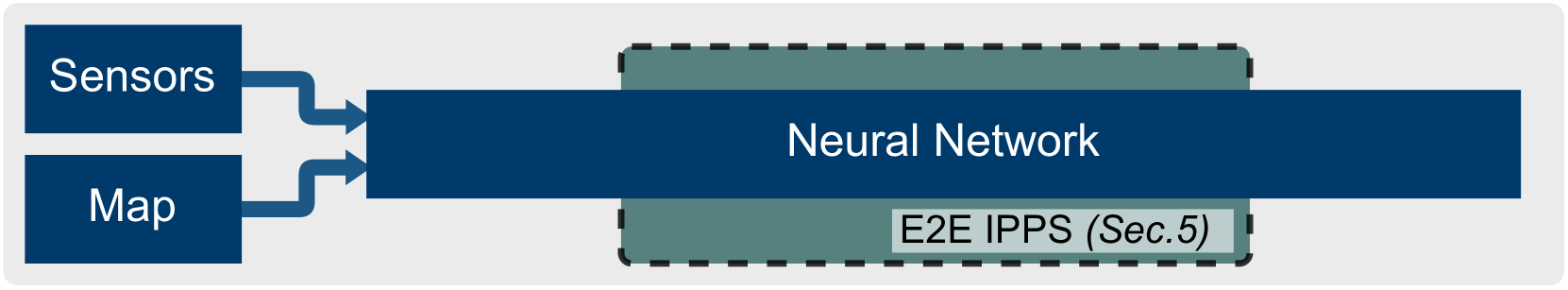
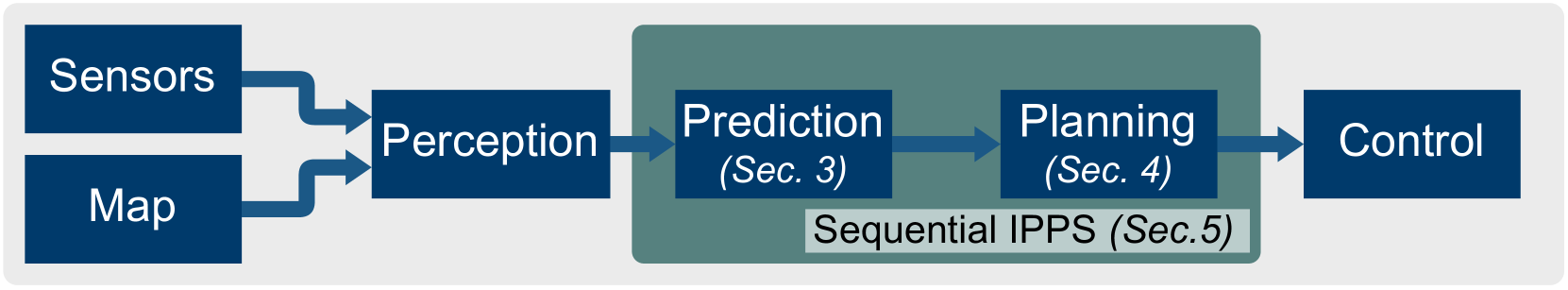
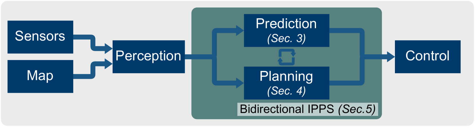
Automated Driving (AD) remains a challenging endeavour. It is usually split into the subtasks of perception, prediction, planning, and control [1, 2, 3]. Perception processes sensor inputs to create a model of the environment. Prediction and planning build upon this model and make future motion forecasts for surrounding traffic agents and a plan for the controlled ego vehicle. Traditional, modular systems (cf. Fig. 1) address prediction and planning as separate tasks. The predicted behavior of surrounding traffic agents is leveraged to plan a suitable behavior for the ego vehicle. However, this sequential ordering is inherently reactive and cannot represent bidirectional interaction between the ego vehicle and other traffic agents [4]. In fact, prediction and planning are no sequential problems and should be tightly coupled in automated driving systems [5, 6, 7].
1.1 Scope
In this work, we review methods to integrate prediction and planning into an automated driving system (ADS).
Prediction is the task of anticipating intents and future trajectories of observed traffic agents [8], and planning is about finding the best possible trajectory w.r.t. previously defined criteria for a controlled vehicle [9].
Deep Learning (DL)-based methods follow a data-centric approach to tackle these problems [10] and have led to significant improvements in many fields [11]. Works in prediction and planning increasingly employ DL-based approaches as well [12, 13, 14, 15] and represent an alternative to traditional, rule-based methods [16, 17] and constrained optimization [18]. In this work, we focus on DL-based methods.
The architecture of an ADS can take different forms, which are shown in Fig 1.
Black-box methods employ a single neural network for perception, prediction and planning (c.f. Fig 1(a)), so that depending on the architecture, no boundaries between the modules can be drawn [9, 19, 20].
In contrast, modular systems consist of clearly defined components for different tasks [21, 22, 23, 24, 25].
Traditionally, they are arranged in a sequential order (c.f. Fig 1(b)).
In this work, we emphasize the shortcomings of this approach and highlight works that integrate prediction and planning in a more sophisticated way (c.f. Fig 1(c)) to enable bi-directional interaction of self-driving vehicles and surrounding traffic.
We refer to the component of an automated driving system that integrates prediction and planning as an Integrated Prediction and Planning System (IPPS).
We limit the scope of our work to mixed traffic without Vehicle-to-X communication between traffic agents.
Furthermore, we exclude pedestrian motion forecasting, which poses a different problem that is subject to weaker dynamic constraints compared to vehicles [26] and has been thoroughly surveyed [27, 28, 29].
1.2 Contribution and Structure
In a thorough approach, this survey first reviews DL-based prediction and planning before focusing on how to integrate these two tasks. While surveys on classical methods [30, 31, 14, 32], stand-alone DL-based prediction [33, 34, 35, 15] or planning [36], and end-to-end (E2E) AD [37] already exist, to the best of our knowledge we are the first to review the integration of DL-based prediction and planning. We summarize our contributions as follows:
- •
-
•
We propose a categorization for the integration of prediction and planning, which addresses model architecture, system design and behavioral aspects. Further, we investigate and analyze the interrelations between these categories and their impact on safety and robustness (Sec. 5).
-
•
We reveal gaps in state-of-the-art research and point out promising directions of future research based on the identified categorization (Sec. 6).
2 Task Definitions
In the following, we start by introducing the terminology and notation for the task definitions used in this work. We adopt a similar terminology to that proposed by [33] and partition the actors in a traffic scenario into the self-driving Ego Vehicle (EV) and the Surrounding Vehicles (SVs). The EV is equipped with sensors that provide information on the environment. The state history of vehicle over the time interval is
| (1) |
Each state comprises 2D or 3D positional information and further optional information like heading angle, speed, static attributes, or goal information in the case of the EV. Hence, denotes the EV’s past states. Similarly,
| (2) |
refers to the past states of all SVs. Analogously, the future states of vehicle within a prediction horizon of are
| (3) |
and the future states of all SVs are .
In the following, state sequences are also referred to as trajectories.
Additional scene information, such as a semantic map or traffic signs and traffic light states are represented by .
Prediction. Following [8], we state trajectory forecasting as the task of estimating a probability distribution
| (4) |
that maps state histories of observed vehicles in to the future trajectories of predicted vehicles in . The distribution accounts for inherent uncertainties in the forecasting task and is often modeled by a discrete set of samples with corresponding probabilities [38, 39, 40, 41]. Some methods omit scene information and infer trajectories based on a state history alone [42, 43, 44].
| Task | ||
|---|---|---|
| , | Single-Agent Prediction | |
| , | Clique Prediction | |
| , | Joint Prediction |
Commonly includes all vehicles in the scene, i.e. and . Depending on the vehicles in , different variants of prediction can be formulated as stated in Tab. I. Single-agent prediction models the future trajectory for each SV individually [45]. However, estimating a joint prediction from a set of single-agent predictions is not trivial since the number of possible combinations grows exponentially with the number of agents . Not all these combinations are meaningful and finding realistic ones with heuristics and joint optimization is cumbersome [46]. To avoid this, joint prediction directly estimates a joint distribution for multiple SVs [47]. As not every single SV interacts with all other actors, ScePT [48] partitions the SVs into highly interactive cliques and models . We only discuss single-agent prediction and joint prediction since clique prediction can be seen as a special case of joint prediction that marginalizes over the remaining SVs. Moreover, the aspects discussed in Sec. 3 are also valid for clique prediction.
Planning. The task is to find a single suitable trajectory for the EV that can be passed on to a downstream motion controller. Hence, we define planning to be a function that maps the observational inputs , and as well as the context information to a future trajectory , i.e.
| (5) |
In many cases, the also uses the prediction , i.e.
| (6) |
The definitions show that planning can be considered a special case of single-agent prediction where the output distribution models only a single trajectory. However, in contrast to prediction, the planning trajectory must be conditioned on a navigation goal. Moreover, it has to be stable in closed-loop, i.e. it must be kinematically feasible and result in safe and efficient driving behavior when fed to a downstream controller.
3 Prediction
The core of prediction is understanding how the driving scene will evolve. Sec. 3.1 discusses how different scene representations allow local and global interactions. Sec. 3.2 reviews which NN designs are used to model interactions and extract descriptive features. Finally, Sec. 3.3 shows how the extracted features are mapped to trajectory predictions and how multimodality is modeled.
3.1 Scene Representation
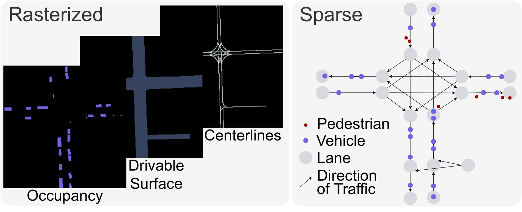
Representing a scene means extracting the relevant subset of all available information and transferring it into a format that subsequent processing steps can utilize. In the context of trajectory prediction for automated vehicles, agent states and map I are the most important information to represent. Two major representations exist in DL-based approaches: Rasterized and sparse (cf. Fig. 2).
Rasterized. Rasterized representations use dense, fixed-resolution grid structures that often have multiple channels [49, 50, 48, 51, 52]. Each channel encodes different information on agent states. They are commonly used in combination with rasterized high-definition maps (HD maps).
Typical modalities are occupancy maps [51], object detections [53], lane markings [54], motion history [55], semantic information [56], traffic signs [57], traffic light states [57], and route information [58] (c.f. Fig 2.
DESIRE [8] is an early work that uses a rasterized representation for DL-based prediction.
A bird’s eye view (BEV) representation is employed to fuse multiple EV sensor inputs into a shared representation.
This allows the combination of different sensing modalities and establishes a common coordinate system for all vehicles, facilitating to model interactions within the scene [59].
Additionally, dense grids are well-suited for processing with powerful Convolutional Neural Network (CNN) [60] architectures [58, 61, 62, 10, 63, 64, 65, 66, 67, 68, 69, 70, 71].
However, embedding all observations in a grid structure leads to information loss due to quantization errors [72].
Moreover, as discussed in Sec. 3.2, the locally restricted receptive field of CNNs can hamper interaction modeling.
Sparse representations use vectors to describe all objects in a scene. The per-object vectors are then either encoded jointly, e.g., with a transformer, or individually and then aggregated, e.g., with Graph Neural Networks (GNN) [73].
Objects are represented by polygons, or point sets [6, 74, 41, 75, 61, 76, 38, 77].
The map is commonly described by a set of lanes represented by polylines and an adjacency matrix.
Objects and map elements are then encoded into fixed-size latent features, for instance, via Multi-Layer Perceptrons (MLP) [78] or Recurrent Neural Networks (RNN) [79, 39].
To encode sequential signals like state histories , 1D CNNs [80], RNNs like LSTMs [81] and GRUs [82], and Transformers [83] are applied [41, 84, 76].
The timeline in Fig. 3 chronologically depicts impactful prediction methods and exhibits a shift towards sparse representations during the past years.
Diehl et al. [72] proposed a graph representation for vehicle interaction modeling.
Based on their work, two approaches emerged: Homogeneous and heterogeneous graphs. Homogeneous graphs encode objects of one class, for example, the road network [74, 41], whereas heterogeneous graphs combine different object classes in one graph [40, 85, 86, 87].
However, their work is focused on highway data and does not include map information.
In contrast, VectorNet [74] proposes to represent all map elements and agents by a set of points.
Agents are represented by a set of points along their motion history, while lanes are described by polyline points. Small objects, such as traffic signs, are represented by a single point, and extended elements are given by polygons defined by multiple points.
Vectornet then processes each object with a homogeneous subgraph called polyline subgraph.
A per-object feature is obtained by max-pooling. Next, all object features are aggregated in a heterogeneous global graph. Finally, the TV trajectory is decoded from the encoding of the node corresponding to the TV.
Trajectron++ [40] and MFP [88] combine rasterized representations for HD maps with sparse representations for objects.
Further, a few works use voxel representations that differ in their degree of sparsity [89], [90].
MultiPath++ [38] is the successor of MultiPath [56] and switches from rasterized to sparse representations. Their results show that the shift from rasterized to sparse can increase performance. The overall development in the field confirms this trend (c.f. Fig. 3).
Coordinate frame. Irrespective of the scene representation itself, the coordinate frame is a fundamental design choice.
Applying a global coordinate system with a fixed viewpoint for the whole scene [91, 46, 92, 6] is computationally efficient.
However, the frame is not viewpoint-invariant, i.e., the predictions change if the coordinate system is moved within the scene.
This leads to low sample efficiency and impairs generalization [93]. Even fixing the coordinate origin to the EV center does not lead to viewpoint-invariant predictions when predicting other agents than the EV [94].
In contrast, other models [95, 96, 74, 54] process a scene from the viewpoint of each agent. Thus, the processing is viewpoint-invariant. On the downside, computational complexity scales linearly with the number of agents and quadratically with the number of interactions [6].
An alternative way to achieve viewpoint invariance are pairwise relative coordinate systems introduced in GoRela [97], which describe the relation between agents instead of using a fixed coordinate frame.
This allows the computation of the relation between static objects offline and greatly reduces computation.
PEP [94] further reduces computation by using center-relative instead of pairwise relative coordinates, i.e. shifting the coordinate frame into the mean position of all processed agents before each transformation.
Another choice to increase robustness are Frenet representations that decompose positions into progress along and lateral offset from a lane [98, 99].
Either a single Frenet frame defined by the target vehicle is used for all agents [100] or each agent is represented in an individual coordinate frame [84, 101].
3.2 Interaction Modeling
A decisive aspect of prediction is to model the interaction between traffic agents represented in the scene [4, 137]. This includes interaction with map elements and other traffic agents. Modeling the relation of vehicles to static map elements like lane markings, traffic signs, etc. is important to understand feasible corridors in which trajectories could be localized. Interaction with other traffic agents are crucial to understanding social interaction.
RNNs. A few early prediction models like DESIRE [8] or Trajectron++ [40] combine RNNs with an aggregation operator like spatial pooling or attention. They either extract temporal per-agent features and then aggregate them across all agents or aggregate information first and extract joint temporal features afterwards.
CNNs. Alternatively, Fast and Furious [102], MTP [54], and Multipath [56] applied 2D convolutions to implicitly capture interaction within the kernel size. Compared to sequence processing-based approaches, higher importance is assigned to spatial interaction.
GNNs and Graph-Attention explicitly model interactions between individual agents by combining multiple agents’ features [138] and processing them with graph convolution operators [139, 73, 140, 141] or graph attention [142, 143, 144, 145] to aggregate information. Prediction networks like VectorNet [74], LaneGCN [41], TNT [75], HOME [104], DenseTNT [106], GOHOME [84], Multipath++ [38], LaFormer [111], and BAT [114] are examples of this development.
Transformers [83] have been widely adopted in prediction: InteractionTransformer [146], mmTransformer [76], AgentFormer [105], SceneTransformer [6], HiVT [108], Wayformer [109], Motion Transformer [110], MotionDiffuser [112], Trajeglish [113] and many further works [147, 148, 149, 150, 110, 151, 152, 153, 154, 155, 156] exploit the global receptive field and attention mechanism of Transformers. All SVs can be predicted simultaneously [76], and the impact of vehicles on each others’ behaviors across different timesteps can be modeled with attention layers [105]. Attention layers can be applied along the spatial and temporal dimension jointly [105], or individually [157]. The latter can be divided into sequential [158, 159] and interleaved [6, 109] architectures. Experiments with Wayformer [109] and SceneTransformer [6] show that joint and interleaved processing outperform sequential approaches. As, joint processing causes higher computational burden, the interleaved paradigm balances best between performance and computational demand.
The timeline in Fig. 3 reflects how interaction models changed together with the scene representation. After CNNs and RNNs were applied to rasterized scene representations in early works, GNNs, attention, and Transformers took over since the advent of sparse representations.
Across all architectures, the prevalent concept is to extend interaction from a local to a global scale. HiVT’s ablation study [108] shows that both, local and global attention, are beneficial for prediction and that hierarchical attention yields the best performance.
3.3 Trajectory Decoding
The final step of prediction is to generate trajectories from latent features. As introduced in Sec. 2, this step models a probability distribution over possible future trajectories given observation and scene context . Here, we focus on two major aspects of trajectory decoding: The modeling of multimodality and the decoding principle.
Multimodality. The intention of SVs is inherently uncertain, making multimodal [160]. Therefore, is commonly either expressed as an explicit density function or estimated with a discrete trajectory set.
Explicit density functions. An intuitive approach to prediction is to explicitly model the probability density function of [61, 66, 69, 70]. Continuous distributions like bi-variate Gaussian distributions [161], Gaussian Mixture Models [110, 162, 132], or discrete rasterized heatmaps [104, 84] can be found in many prediction works. Alternatively, object-agnostic representations like occupancy maps [53, 163], or flow fields [164, 165, 70] can be used. These representations handle multimodality implicitly [61] and were shown to be more robust against perturbations [62]. However, since no discrete trajectories are decoded, it is difficult to compare such representations with expert logs for performance evaluation.
Discrete trajectory sets are either created by sampling from an intermediate distribution or by the model design.
To sample a diverse trajectory set from an intermediate distribution, generative models such as Generative Adversarial Networks (GANs) [166], Conditional Variational Autoencoders (CVAEs) [167], normalizing flows [168] or denoising diffusion [112], can be used [8, 89, 169, 170, 171].
Alternatively, recent methods apply several prediction heads to the features extracted by a common backbone to decode a set of diverse trajectories [38, 41, 172, 109].
Other ways to obtain diverse predictions are training loss functions [75], entropy maximization [39, 173], variance-based non-maximum suppression [174], greedy goal sampling [55, 97], divide and conquer strategy [175], evenly spaced goal states [176], or with pre-defined anchor trajectories [56, 177]. Nevertheless, a guarantee of coverage can only be given by specifying high-level behaviors [124] or regions of the map that must be covered by at least one prediction [76].
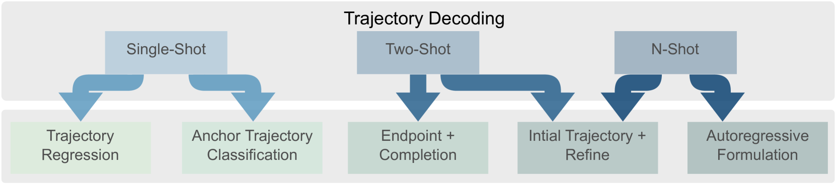
Decoding principles. We classify the decoding principles into one-shot, two-shot, and n-shot methods as depicted in Fig. 4. While it is a common practice in planning to decode trajectories as a sequence of actions that translate into Cartesian space using a kinematic model (cf. Sec. 4.2), only a few works do so in prediction [178, 179]. Instead, future waypoints are predicted directly from latent features [41, 38, 111, 109, 180].
Single-shot approaches are split into trajectory regression and anchor trajectory classification.
Trajectory regression directly decodes the latent features to a trajectory using a NN, typically an MLP [54, 74, 41, 38, 6, 107, 108, 109].
Especially Transformer-based architectures use direct trajectory regression decoding (cf. Fig. 3). However, these methods are prone to predict trajectories that leave the road, cut corners, or are kinematically infeasible [97].
Specifically designed loss functions for offroad driving [181, 182, 39, 183, 184], driving direction compliance [185] or distance to the centerline [186] can alleviate the problem.
Anchor trajectory classification states prediction as a classification task.
Thus, a probability is estimated for a set of pre-defined trajectories [55, 177]. Defining anchor trajectories can ensure the feasibility of the prediction and allows to impose hard kinematic constraints. However, rare trajectories might not be covered by the anchors.
Two-shot methods structure trajectory decoding into meaningful subtasks that increase explainability and are more flexible than anchor trajectory classification. They comprise endpoint and completion as well as initial trajectory and refine strategies.
Endpoint and completion methods are based on the assumption that a trajectory is mostly defined by its endpoint [25].
The endpoint can either be regressed [104], [84] or classified from a pre-defined set [75], [106], [97]. Usually, classification-based methods additionally regress an offset of the classified endpoint [75]. HOME [104] estimates the endpoint probability distribution as a rasterized map, samples potential endpoints, and then regresses the trajectory using an MLP.
Initial trajectory and refine approaches combine the ideas of anchor trajectory classification and endpoint and completion. Instead of an endpoint, an initial trajectory is classified or generated. Then, a refinement step adapts the trajectory, for example, by offset regression for each predicted waypoint [102, 56, 111].
TPNet [187] and DCMS [188] first regress an endpoint, then generate trajectory proposals and finally refine them.
N-shot methods are either initial trajectory and refine or autoregressive formulations.
Initial trajectory and refine strategies in their n-shot variants are similar to the two-shot version. The only difference lies in the refinement step, which is realized as a recurrent optimization [8, 112]. For example, MotionDiffuser [112] samples a noisy trajectory and repeatedly applies denoising diffusion to refine the trajectory.
Autoregressive approaches use recurrent decoding to perform a stepwise roll-out into the future. Iteratively, the next waypoint is predicted, and information on the resulting scene is added to the latent features [103, 189, 40, 76, 105].
Autoregressive decoding can help to enforce high-quality social interactions and scene understanding [97] but might lead to compounding errors since predicted information is used to make further predictions [190]. Further, the computational effort and computation time of these methods are usually higher than for one-shot or two-shot methods.
Fig. 3 shows the development of trajectory decoding using the categories defined in this Section. While endpoint and complete decoding gained popularity, auto-regressive formulations were recently used less often, assumingly due to computation time deficiencies. Trajectory regression decoding was always used but became prevalent with the rise of Transformer-based interaction modeling in prediction.
3.4 Benchmarks
Various prediction datasets provide training, validation, and test splits for benchmarking. The most prominent ones are nuScenes [191], WOMD [192], Argoverse [193], Argoverse2 [194], inD [195], highD [196], rounD [197], exiD [198], and Interaction [199]. Evaluation is carried out by comparing the predicted trajectory of an SV to its ground truth future trajectory. To account for the inherent multimodality benchmarks are commonly based on a winner-takes-all evaluation. This means the model predicts a fixed number of output trajectories, e.g., six [194] or ten [191], and the evaluation takes only the best one among them into account. Alternatively, predictors that output a parametric distribution are often evaluated based on the Negative log likelihood (NLL) of the ground truth under the predicted distribution. This assessment also factors in the uncertainty predicted by the model and evaluates the whole distribution instead of only a single trajectory.
4 Planning
The planning task is to find a trajectory for the EV that factors in safety, comfort, kinematic feasibility, and goal-directedness based on the observations and as well as additional context and optionally (cf. Sec. 2). In this section, we will first give a comprehensive overview of common input (Sec. 4.1) and output representations (Sec. 4.2). Then, we address goal-conditioning in Sec. 4.3 before we categorize existing works and discuss common paradigms in Sec. 4.4. Finally, we briefly describe existing benchmarks in Sec. 4.5.
4.1 Input Representation
We classify planning input representations into interpretable intermediate representations and latent features.
Interpretable intermediate representations such as rasterized or sparse scene representations (that were discussed thoroughly in Sec. 3.1) are common inputs to planning components in modular ADSs. Thus, many works exist that build on rasterized [58, 67, 124, 200] or sparse inputs [125, 131, 201, 130, 24]. Similar to prediction, a clear trend can be observed from rasters to sparse inputs.
Latent features. E2E ADSs directly map sensor information to actions (cf. Fig. 1) [9, 202, 20]. Thus, instead of , , and , the planner’s inputs are latent features.
The benefit of using learned latent intermediate representations is that no manual engineering effort is needed to design the interfaces between different modules.
The main drawback of hand-engineered interfaces is that they have to apply to the long-tailed distribution of potential driving scenarios, and every piece of information discarded by the interface cannot be recovered. For instance, if a vehicle is currently occluded, but its presence can be inferred from the reflection of its headlight in another car, bounding box representations [58], occupancy fields [70], or affordances [115, 119] will not be able to propagate this information to downstream modules [203, 133].
In contrast, latent feature representations allow uncertainty propagation, enabling downstream modules to compensate for errors at earlier stages, such as undetected vehicles [61].
The main disadvantage of latent feature representations is the lack of interpretability.
In case of failures, evaluating which part of the system caused the error is extremely difficult.
This aggravates tuning and debugging of pure E2E systems.
Interpretable E2E systems seek to compensate for this by producing additional intermediate representations [66].
In contrast to modular stacks, these interpretable intermediate outputs are not used by the planner.
Instead, they are only used for additional supervision and model introspection.
The timeline in Fig. 3 reveals that interpretable input representations are becoming increasingly popular compared to latent input features.
4.2 Output representation
The planning output is typically represented as a sequence of future states or control actions.
Future states are given by a sequence of future 2D position and heading angles representing the planned trajectory of the EV over time [22, 62, 58]. This trajectory is then passed to a downstream controller tasked with tracking it [22]. The trajectory representation is well interpretable and can be easily checked for collisions, traffic law violations, or deviations from the driveable surface [129, 68]. Moreover, it is agnostic of the kinematic parameters of the controlled vehicle, enabling generalization to other vehicles. However, the ultimate driving performance also depends on the downstream controller and how well the planner and controller are tuned for each other. Validating and testing the system can require iterations between both components, which slows down development.
Future actions are an alternative representation of planned behavior.
This is mostly adopted by E2E ADSs that regress acceleration and steering angle without the intermediate trajectory representation [117, 118, 119].
Besides ensuring kinematic feasibility, it can promote comfort as it is directly related to the magnitude of the actions.
However, the resulting behavior depends on the controlled vehicle’s individual dynamics [204, 19].
Hence, generalization to other vehicles is limited.
Fig. 3 depicts that early E2E ADSs planned in actions, while trajectory outputs recently gained popularity.
4.3 Goal Conditioning
The overall task of ADSs is to navigate safely toward a destination. Hence, goal-directedness is one main criterion that determines the suitability of a potential plan. Lane-level route information can be provided to the planner by a navigation system. Popular benchmarks provide route information through a high-level command such as ’turn left’ or ’go straight’ [205], through sparse goal points along the route [205] or by annotating lanes within the map as on-route or off-route [206]. For example, in the widely used Carla simulator [205], goal locations are sparsely sampled along the route, and in each planning step, the closest goal location is provided to the planner. We define four categories to describe how this goal information is incorporated into the planning algorithm: input features, separate submodules, routing cost, and route attention. While the first two were originally introduced in [117], the latter were proposed more recently [201, 207, 126, 208].
Input features are the most straightforward way to incorporate goal information and have been widely adopted [120, 20, 124, 209, 210, 24, 63, 64, 118, 23, 122].
Different methods exist to pass this input to the planning module depending on how the route information is represented.
If the lanes within the map information are annotated as on-route or off-route, then this information can be used as a separate semantic channel in raster maps [58]. Similarly, vector inputs describing the lane centerlines can have an additional flag reflecting this information [201].
High-level commands were used as input feature in LBC [124], LAV [67], and AD-MLP [208].
It was found that inputting high-level intention repeatedly at different stages of the network increases its generalization capability [23].
Transfuser [20] leverages sparse goal locations as 2D features in the final trajectory decoding step.
While using goal information as an input feature is simple, goal compliance is not guaranteed.
On the contrary, [201, 117] demonstrated that the model could ignore this additional input and instead rely on other potentially spurious correlations, such as between the current and the future kinematic state.
Separate submodules are used only with high-level commands, which serve as a switch between command-specific submodules [117, 70]. Balancing the dataset to prevent it from being dominated by a single driving mode, such as lane following, is avoided in this setup, as each block is only trained on a single high-level command. However, this approach requires a fixed number of high-level commands to be defined in advance.
Routing cost. A third option is to plan trajectories by optimizing a cost term for routing [66, 69, 62]. Such cost functions can measure the remaining distance to a goal location [62], the progress along or distance to an on-route lane [66]. Goal-directedness is balanced with further competing objectives such as safety and comfort. Thus, the planner can flexibly react to difficult situations, e.g., it could drive off the road to prevent a collision. However, tradeoffs between safety and comfort versus progress can be undesirable.
Route attention applies spatial attention to relevant parts of the map, i.e., the route. This can be achieved by removing the off-route portion of the map from the input features, e.g., PDM-Open [126] and PEP [94] discard almost the entire map information and only keep points along a lane centerline on the route. Similarly, GC-PGP [201] removes off-route nodes from the lane graph after information aggregation and TPP [134] and DTPP [136] discard all EV trajectory proposals that do not comply with the route.
Fig. 3 shows that early models did not condition their plan on a goal at all. Afterward, submodules and input features dominated. While using input features is easy to implement, it is less effective, whereas submodules represent a major architectural constraint. The most interpretable method is using a routing cost function. Recent models introduced route attention, which is more flexible. Both route attention and routing cost allow to condition on goals that are not reflected in the training dataset, thus improving generalization.
4.4 Planning Paradigms
Recall that in Eqn. 5 we defined planning to be a function mapping from observational inputs , , and predictions to a trajectory . In the following, we focus on the planning function . To this end, we decompose into two parts: A proposal generator , yielding a set of multiple potentially suitable trajectories and a proposal selector that selects the final plan among the proposed set. Hence, in this work, we propose to represent the planning function as
| (7) |
Based on this, we distinguish three different paradigms adopted for the planning task: Cost function optimization, regression, and hybrid planning.
Cost function optimization. As planning aims to find a trajectory that optimizes objectives such as safety, comfort, and progress, it is a natural approach to design and optimize a cost function that balances these potentially conflicting objectives. Cost function-based planning methods [121, 61, 211] rely entirely on the selection function to find a suitable trajectory, i.e.,
| (8) |
where is a cost function of the planned trajectory.
Consequently, the proposal generator may randomly sample feasible motion profiles [61] or obtain them by clustering real-world expert demonstrations [70].
Traditional non-learning-based methods rely on hand-crafted cost functions [212, 213, 214, 215, 216, 217, 218, 123].
However, designing a cost function that effectively balances these goals and generalizes to the long-tailed distribution of possible driving scenarios is challenging.
Learning-based methods aim to address this by learning a cost function directly from expert demonstrations [219, 220, 103].
Similarly, [119, 115] learn to regress driving-relevant affordances such as the distance to the leading vehicle or the heading angle relative to the lane, based on which a downstream controller infers driving commands.
The learned cost function can be non-parametric [61, 221, 222] or comprise hand-designed sub-costs of which only the weights are learned [69, 70, 66, 121].
The non-parametric cost function of the NMP [61] assigns a cost to each potential future EV position within the planning horizon and is represented as a 3D-BEV-Tensor.
In contrast, hand-designed sub-costs commonly evaluate safety, comfort, traffic rule compliance, and progress [121, 70, 66].
Regression approaches rely entirely on the proposal generator . The selection function is the identity, and all burden is placed on the proposal generator , which only generates a single proposal . E2E methods fall into this category. Regression approaches can learn to directly predict future waypoints [201, 20, 24] or actions [9] by supervised learning [223]. This form of imitation learning, i.e., supervised learning from expert data, is called behavior cloning (BC) [224, 190, 225]. This approach makes the manual design of the cost function obsolete. However, BC models are vulnerable to distributional shifts, which occur when the model reaches states not covered by the training data. Besides, regressed trajectories are generally not guaranteed to be kinematically feasible. UrbanDriver [24] counters this by training the model directly in a closed-loop simulation. However, this requires the entire simulator to be differentiable. CW-ERM [226] rolls out the policy in a non-differentiable simulation to identify important training scenarios and assign sample weights.
Hybrid planning describes methods that combine both ideas. First, a set of candidate trajectories is regressed by the proposal generator , then the best one is selected with a cost function in [227]. For instance, [130, 131, 228, 229, 132] perform collision checks on the proposed trajectories to rule out unsafe proposals. In this setting, it often remains unclear which parts of the overall objective are enforced by the proposal generator and which by the cost function.
Fig. 3 shows that regression is the dominating planning paradigm for E2E systems. Cost function-based planning is mainly used in the work of researchers from Uber ATG and the University of Toronto [68, 66, 69, 70].
4.5 Benchmarks
Different methods exist to evaluate planning approaches, namely open-loop evaluation and closed-loop simulation.
Open-loop evaluation is similar to an evaluation in the prediction task. It compares the planner output to that of an expert planner [230]. However, this does not give the planner control over the EV and ignores the problems arising from compounding errors and distributional shifts [231]. More severely, recent work demonstrated that open-loop evaluation results do not correlate with driving performance [126, 232].
Closed-loop simulation in contrast, lets the planner control the EV. Instead of merely comparing the planner output to that of an expert planner , the evaluation is based on metrics for comfort, safety, and progress. Thus, closed-loop evaluation relates better to real-world driving but requires a simulator to let the model interact with its environment. Prominent simulators are Carla [205], nuPlan [206], Waymax [233], Highway-Env [234], and CommonRoad [235]. Carla is a high-fidelity simulator that involves sensor simulation, whereas nuPlan, Waymax, CommonRoad, and Highway-Env operate on abstract object representations (e.g., bounding boxes) without rendering camera or lidar sensors. Many benchmark datasets were proposed for the Carla simulator [232, 236, 237, 20]. However, the scenarios are purely synthetic, which questions the generalizability to the real world. In contrast, nuPlan and Waymax follow a data-driven approach, which uses recordings from real-world scenarios to initialize the simulation. Thus, users have access to corresponding large-scale real-world datasets to train their method before deploying it in simulation. CommonRoad is compatible with several smaller datasets [195, 196, 197, 198, 199]. Highway-env is based on simplistic synthetic environments.
When simulating regular driving scenes, rare and critical scenarios are naturally under-represented. This problem can be tackled with data curation [238, 239] or additional test case generation. These can be generated manually [240, 241, 242, 243, 244, 245] or automatically from recorded driving logs [246, 247, 248]. Other methods generate adversarial critical scenarios by augmenting actors within the scene [249, 250, 251, 252, 253, 254, 255, 256] or the scene itself [257, 258, 259, 260, 261]. Similarly, [5, 64] investigate human-robot interaction more closely with hand-crafted scenarios – an aspect that is uncared for in average driving situations.
Another major challenge in closed-loop evaluation is to realistically simulate the SVs. Simple simulators such as Highway-Env [262] rely on non-reactive agents that follow predefined trajectories [263]. In the non-reactive version of nuPlan, and Waymax, these trajectories are obtained from real-world recordings. However, if the EV behaves differently than the expert during recording, this can result in collisions caused by the SVs, as they do not react to the EV. Hence, this simulation is usually limited to short sequences, where the EV stays close to the expert’s trajectory [264]. Carla, nuPlan, and Waymax also provide a reactive driver model for the SV, such as the Intelligent Driver Model (IDM) [16, 17, 265, 266, 267, 268]. Another line of work focuses on learning-based methods to simulate realistic driving behavior [269, 270, 271, 272, 273, 274]. In Waymax [233], users can plug in their own model to control objects in the scene.
5 Integrating prediction and planning
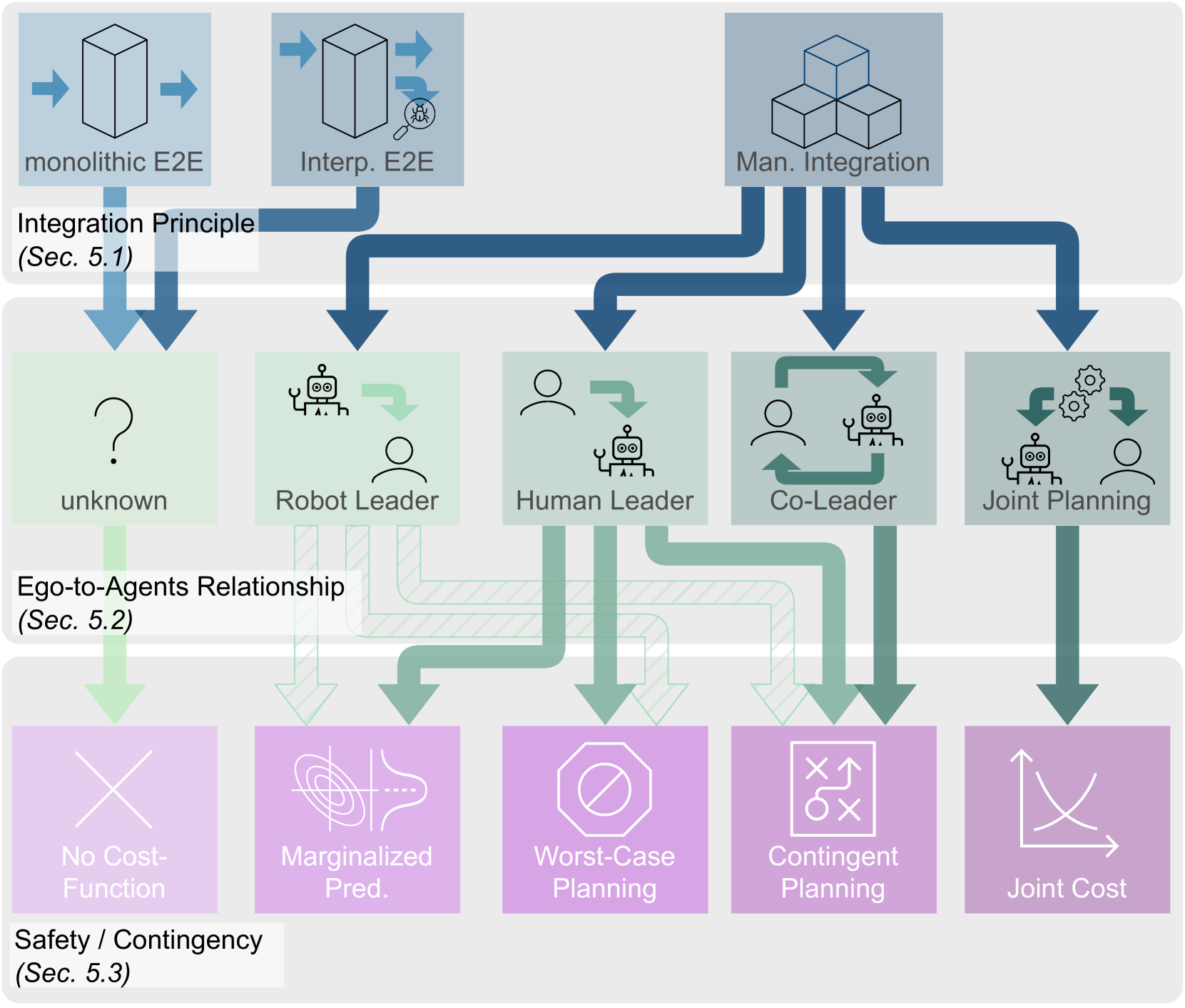
After reviewing key aspects such as interfaces and architecture of planning and prediction components found in ADSs, we change perspective and discuss the properties of the IPPS. In particular, we will highlight the influence of design decisions in the IPPS on behavior in interactive scenarios. We will start by categorizing existing works based on which components the IPPS comprises (Sec. 5.1). Then, we will describe the implications for the interactive behavior which follow from design choices in modular integrated systems (Sec. 5.2). Subsequently, different concepts of safety and contingency in modular integrated systems are discussed in Sec. 5.3. Finally, Sec. 5.4 discusses possible combinations of these categories. An overview is provided in Fig. 5.
5.1 Integration Principles
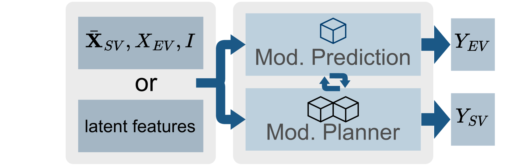
In this work, we distinguish among three design principles for IPPS. An overview can be seen in Fig. 6.
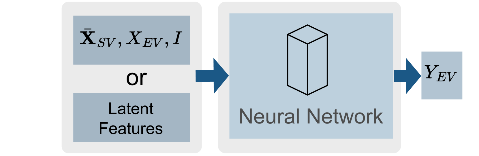
Monolithic E2E planning describes methods where the IPPS consists of a single E2E planner, which maps the state inputs , , and to the EV’s trajectory .
Thus, the SVs’ future behavior and the interactions among them, as well as between the SVs and the EV, are not modeled explicitly.
However, the expert’s actions, which the E2E planner learns to imitate in training, are based on reasoning of how the future will unfold.
By learning to imitate actions, the model could exhibit behavior that is implicitly based on such reasoning as well.
For instance, consider a scenario where the EV’s leading vehicle brakes.
An expert or a human driver will base their driving decision on the likely future scenario that the safety margin will shrink and thus brake as well.
Hence, an E2E planner that imitates the expert’s behavior makes a decision that is implicitly based on a predicted future.
Pioneered by Pomerlau [9], there is a vast body of literature on IPPS based on monolithic E2E planners [19, 116, 117, 118, 22, 62, 10, 63, 64, 23, 67, 122, 236, 24].
The main disadvantage is their black-box nature, which makes model introspection and safety verification difficult.
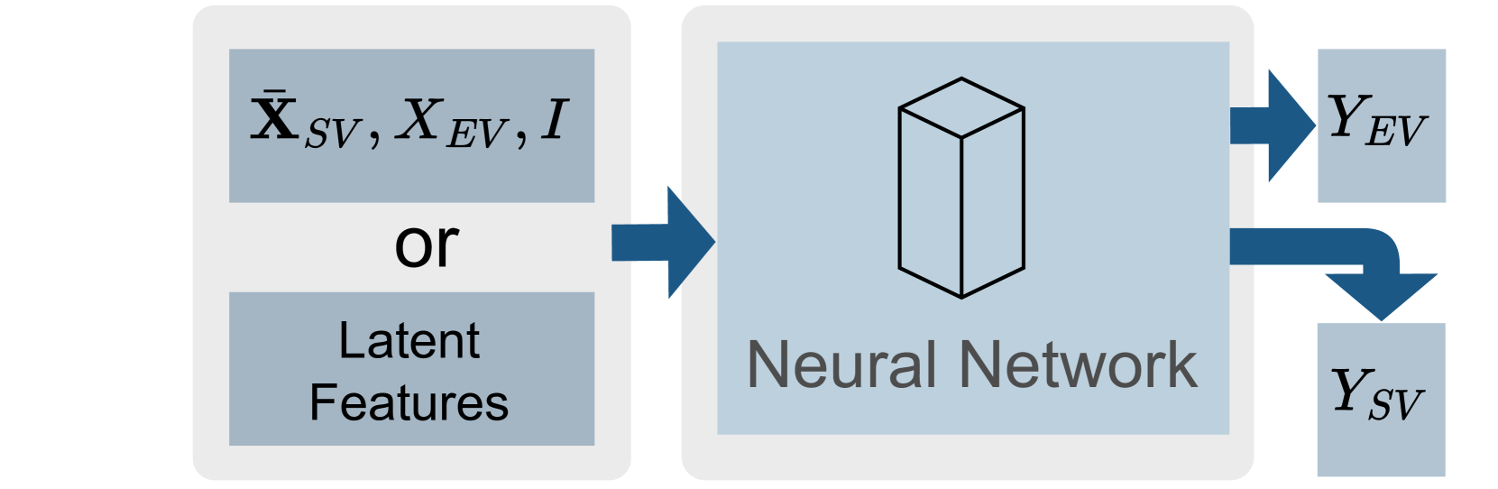
Interpretable E2E planning frames prediction as an auxiliary learning task [58, 61, 120, 125].
Explicit predictions are an additional model output trained jointly with the planning task.
Usually, a shared backbone encodes features that are used for both tasks.
Then, separate heads decode the respective output representations.
The additional objective provides a learning signal to the backbone.
It acts as a regularization which can make the learning process more sample-efficient and can increase generalization capabilities [58, 124, 119] as it was previously demonstrated for other auxiliary tasks in prediction and planning like speed prediction [64], semantic mapping [275], and occupancy forecasting [66].
However, the additional learning objective results in a trade-off between the different tasks, usually resulting in a hyperparameter that balances the respective losses and has to be tuned empirically.
Compared to monolithic E2E planning, the explicit prediction adds interpretability and facilitates introspection. Nonetheless, both IPPS designs cannot provide safety guarantees.
Hence, we attribute the increased driving performance to the regularizing effect of the additional objective.
Manual integration of a planner with a prediction module means that a separate subsystem is employed for each of the tasks. The interplay of both tasks is manually engineered based on domain knowledge. The most widely adopted integration is a sequential pipeline, where first the prediction module is inferred, and its output is fed to a subsequent planning module [70, 66, 69, 123]. Since this design is unable to reflect the impact of the EV’s plan on the SVs, an alternative is to swap the order of prediction and planning: First, candidate plans are generated, followed by a conditional prediction module. Then, the best plan for the EV is selected among the candidates [129, 134]. Alternative methods iterate between prediction and planning [276] or do both jointly [132]. In the following, we give a chronological overview of different models and highlight the integration design of prediction and planning.
PRECOG [65] uses a probabilistic model for conditional multi-agent forecasting. It implements autoregressive trajectory decoding for EV and SVs jointly. At each time step, the state of all agents is updated and used as input for all other agents in the next update step.
PiP [129, 277] reverses the view of IPPS. Its core idea is that SVs behave differently depending on the EV’s actions. A trajectory generator provides a set of candidate plans independent of the SVs. Each candidate plan is then used to condition prediction. Finally, the optimal plan is selected using a cost function.
DSDNet [68] combines E2E and modular model design. Each of the sequential NN modules additionally has access to the high-dimensional features of the perception backbone, complying with the hypothesis [20] that scene context is important for robust planning. For each detected vehicle, a set of potential future trajectories is predicted. To select the plan for the EV from a sampled candidate set, a hand-crafted cost function is applied, which quantifies the collision probability of the EV candidate trajectories and the SVs’ predicted trajectories.
P3 [66], LookOut [69], and MP3 [70] use cost functions to link prediction and planning. P3 predicts an occupancy map, LookOut [69] employs predicted trajectories to evaluate different pre-defined EV candidate trajectories. MP3 [70] extends P3 into a mapless approach by predicting an online map. A ’dynamic state map’ comprising detections and prediction is used together with the intended route to evaluate potential trajectories.
SafetyNet [130] parallelly applies a monolithic E2E planner with implicit prediction and an explicit prediction module. Multiple collision checks between EV plan and SVs predictions are performed. If the initial plan is classified as unsafe, a hand-crafted fallback layer generates a lane-aligned trajectory. SafePathNet[131] improves upon SafetyNet [130] with a transformer module for joint prediction and planning. In a mixture-of-experts approach, multiple modes are predicted and ranked. The ranking is updated by checking for collisions with the most probable SVs’ predictions. Finally, the highest scoring EV mode is selected.
DIPP [7] jointly predicts the trajectories for all agents, including the EV, which is treated as an SV. The mode with the highest probability is selected for each vehicle. A differentiable nonlinear motion planner then performs iterative, local optimization under consideration of a kinematic model and a hand-crafted cost function.
Inspired by hierarchical game-theoretic frameworks [278, 279, 280, 281], GameFormer [132] models interaction between agents as a level- game [282, 283]. Thus, a transformer decoder models the interaction between all agents, including the EV, by iteratively updating the individual predictions based on the predicted behavior of all agents from the previous level. Hence, the model yields a joint prediction for all agents, including the EV.
UniAD [133] implements a modular system that is trained E2E based on the planning objective. Queries are used as the interface between the submodules so that the planning module can attend to agent-level features from previous network layers. Various works adapted or extended this approach: VAD [135] and Hydra-MDP [284] use the output of previous layers explicitly for collision and map compliance checks. PPAD [276] repeatedly iterates between prediction and planning based on the perception modules’ outputs and GenAD [285] adapts a generative decoder to regress SV and EV trajectories jointly.
TPP [134], DTPP [136], and MBAPPE [286] represent multiple future outcomes in scenario trees, where branches reflect combinations of SV predictions and EV plans. The best plan is obtained through a tree search.
Compared to other integration principles, manual integration requires more engineering effort but restricts the solution space in a meaningful way by incorporating prior knowledge. Often, manually integrated IPPS provide a high explainability and safer plans than E2E systems [287, 131].
The timelines in Fig. 3 show how early works relied mostly on implicit predictions in monolithic E2E designs. Starting with ChauffeurNet [58] and PRECOG [65], explicit predictions became more popular. More recently, manual integration of E2E differentiable modular components gained popularity [203, 133].
5.2 Ego-to-Agents Relationship
After reviewing the integration principles from a system architecture perspective, in the following, we will analyze the manual integration category from a different perspective, namely the intended ego-to-agents relationship.
This is of special importance in highly interactive scenarios since the EV needs to base its driving decisions on the observed and expected behavior of surrounding agents.
However, as [5] pointed out, the EV also needs to be aware that it can influence the behavior of others.
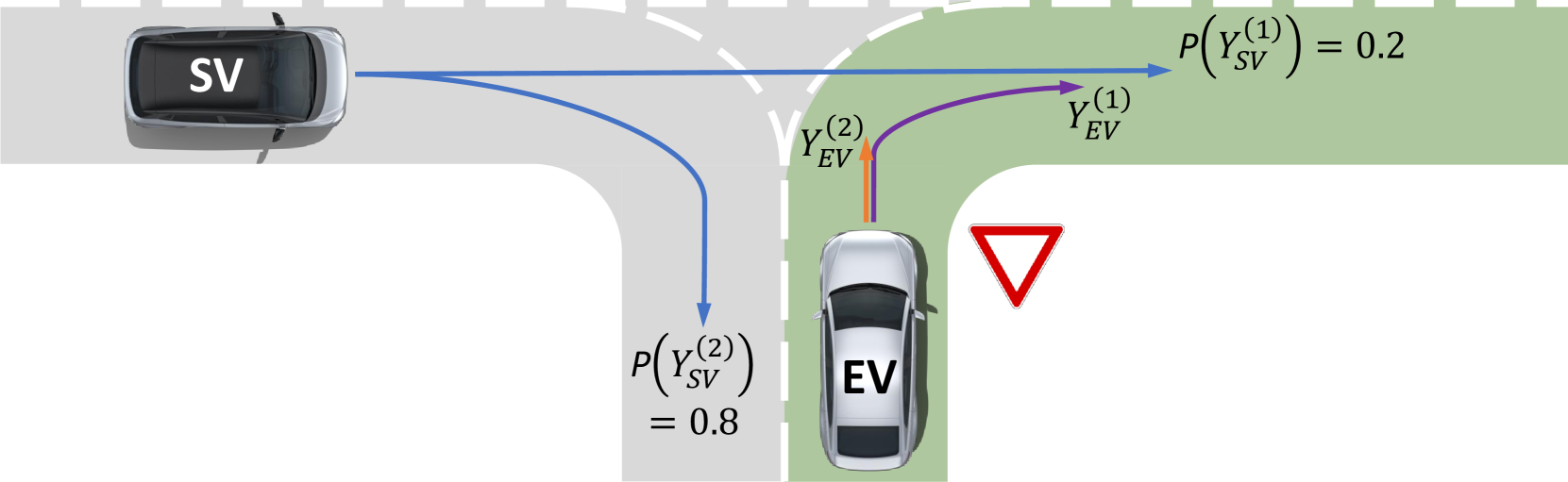
For instance, in the example in Fig. 7, the plan of the EV can also influence the behavior of the SV: If it approaches the intersection faster, the SV might decelerate and yield to the EV.
To describe if and in which way the mutual interaction of the EV and surrounding traffic is taken into account in the planning step, [5] introduced the following four categories: robot leader planning, human leader planning, co-leader planning, and joint planning.
In this context, human refers to the surrounding traffic, and robot refers to the self-driving vehicle.
In the following, we briefly describe these categories and discuss existing work.
Robot leader planning. The EV plan is inferred based on the current state, and the prediction step for the whole environment is conditioned on it. Hence, the EV can effectively seek to make the SV react to its trajectory [88, 128, 127]. This can result in aggressive driving behavior. For instance, in the example in Fig. 7, the EV would reason that when it follows the fast-progressing plan, the observed SV will yield to it to prevent a collision.
Human leader planning is the opposite of robot leader planning. The plan is based on the forecasted behavior of SVs [61, 62, 70, 66]. Hence, the EV shows a reactive behavior. It does not model the influence of the EV’s plan on the SVs, which can lead to underconfident behavior [5]. This is the case for IPPS that predict and plan sequentially. In the unprotected right turn example (cf. Fig. 7), the EV tries to find a plan that is suitable given the two predicted SV behaviors without being aware that it can influence them. Consequently, it will favor the slower plan.
Joint planning describes systems that are aware that vehicles (including ego) interact with each other. The EV’s plan is obtained by global optimization over all agents [288]. Hence, the IPPS system deterministically approximates a joint objective [289] under the assumption that an optimal outcome exists. Hence, it erroneously assumes that the behavior model used for SVs is exactly known and that every traffic participant optimizes this same global objective. For example, if the EV in Fig. 7 squeezes in before the approaching SV, this may be optimal with respect to a reasonable global objective. Nonetheless, there is no guarantee that the SV will behave accordingly. Consequently, [5] demonstrates how this can lead to fatal errors.
Co-leader planning is the most complex paradigm. It models the influence of SVs’ potential future behaviors on the EV plan as well as their reaction to potential ego trajectories [290, 291, 5]. In contrast to the joint planning category, the surrounding agents’ behavior is not assumed to be deterministic. The EV has to consider this uncertainty in the planning step, e.g., by being prepared for multiple future outcomes and reacting accordingly. Additionally, co-leader planning expects the SV to make plans for different potential behaviors of the EV. The EV can exploit this by behaving in a way that makes the SVs reveal their intention, which in turn lets the EV make more confident plans. For instance, in the example in Fig. 7, the EV can try to slowly approach the intersection to provoke a reaction of the SV. This reaction can either indicate that the SV is going to make a turn, e.g., with a turn signal or by slowing down, or the opposite, i.e., accelerating, to indicate that the SV will continue straight. The former will enable the EV to confidently decide in favor of the faster-progressing plan. CfO [5] originally introduced this paradigm, leveraging normalizing flows to represent multi-agent behavior as a learned coupling of independent variables. However, the intricate nature of this architecture may pose obstacles to wider adoption. Furthermore, their benchmark is simplistic, encompassing only a few scenarios with hard-coded agent behaviors. TPP [134] presents a readily comprehensible tree-structured framework that implements co-leader planning. It involves sampling kinematically feasible trajectories for the EV and then conditioning prediction on each of them. An autoregressive formulation for prediction ensures causality: It can be seen as a way to roll out the scene with SV predictions and the EV plan such that both can only access the observation history up until the respective rollout step. Finally, the best EV trajectory proposal is selected with a dynamic programming algorithm. DTPP [136] extends this with a transformer-based conditional prediction module, which allows the forecast of all agents conditioned on multiple EV plans at once. It also replaced the dynamic program with a learnable cost function and applied node pruning to reduce computational burden. Still, the EV reaction to the prediction is taken over entirely by the cost function because the sampled ego-proposals are non-reactive with respect to the SV predictions.
Fig. 3 shows that no clear trend toward one of the paradigms can be observed. While Co-leader planning is theoretically the most capable paradigm, it has not yet been shown empirically if one of these four theoretical concepts is superior to the others and how it can be realized in the design of system architectures. This may also be related to a lack of comprehensive empirical benchmarking focused on interactive behavior.
5.3 Safety and Contingency
The ego-to-agents relationship categories discussed above highlighted that considering multiple potential future scenarios is essential to safety and contingency planning. In the following, we will discuss how this can be incorporated into the cost function component that we defined as part of the planning function (cf. Sec. 4.4). We will analyze the implications of different design choices on safety and contingency. To this end, we introduce the following notation: We denote the number of relevant future scenarios with . These scenarios can be reflected by a multinomial distribution describing the behavior of SVs in each scenario. Based on how this distribution is reflected in the design of the IPPS, we form the following three groups of existing methods regarding safety and contingency: Planning with marginalized predictions, worst-case planning, and contingency planning. They are briefly outlined in Fig. 7.
Planning with marginalized predictions describes IPPS that do not explicitly distinguish multiple future scenarios . This means that the prediction is marginalized over the future outcomes . This can be done explicitly, i.e., by integrating over the scenario probabilities
| (9) |
or implicitly, i.e., by representing all possible scenarios in a joint representation instead of differentiating scenarios. For instance, IPPS that incorporate the prediction in their cost function and do not consider separate future outcomes when evaluating a proposal fall into this category [61, 70, 66]. Hence, their selection function takes the form
| (10) |
Similarly, this is the case for all systems in the monolithic E2E category (cf. Sec. 5.1) [201, 20, 24, 9, 19], as they do not explicitly consider multiple future scenarios and hence – if at all – learn marginalized predictions. Broadly speaking, this means that the IPPS assumes that all scenarios will occur to a certain degree at the same time. As can be seen in the example of Fig. 7, the cost function needs to trade off unlikely but dangerous scenarios (e.g. collision) against very likely low-cost scenarios. This is safety-critical since planners need to be cautious, especially w.r.t. unlikely but dangerous events.
Worst-case planning refers to IPPS that are aware that multiple future outcomes exist. In this category, no probabilities are considered. Instead, each proposal is evaluated based on the worst-case scenario. The motivation behind this assumption is that the final output trajectory must be safe in each possible scenario. Consequently, the selection function can be formulated as
| (11) |
This paradigm strongly focuses on collision avoidance and can result in overly conservative behavior, as shown in Fig. 7. While this assumption is not a popular choice in DL-based prediction and planning, it is broadly applied for rule-based safety layers such as RSS [292] and can be seen as an intermediate step between planning with marginalized predictions and contingency planning.
Contingency planning prepares for the unknown future development of the scene by taking into account different future scenarios and their probabilities . The resulting plan hedges against worst-case risks while enabling progress in expectation. Both the cost function-based and the hybrid planning paradigm can have these properties, and the selection function takes the general form
| (12) |
where is a contingent selection function.
For instance, [69, 287, 293] find a plan that is safe for scenarios on the short horizon (independently of their probability, i.e., worst-case) and also optimize the expected cost on the long horizon (marginalization). Thus,
| (13) |
where and consider the short-term and the long-term part of the proposal , respectively. In the example in Fig. 7, this planner allows the most progress while still ensuring safety. CfO [5] further differentiates between passive contingency where the EV is contingent upon the SVs [69, 287, 293, 294] and active contingency where the EV also expects the SVs to be contingent upon it [290, 291, 295].
5.4 Possible Combinations
In the previous sections, we have described three ways to categorize the integration of prediction and planning methods, namely (1) integration principle, (2) ego-to-agents relationships, and (3) safety and contingency. In the following, we discuss possible combinations of these three dimensions. Fig. 5 shows an overview. Our key insight is that the categories we characterized describe the differences between IPPS methods on different levels. While the integration principle focuses on a high-level system architecture, the ego-to-agent relationship is mostly based on interactive behavior. The safety and contingency consideration is founded on the cost function, i.e., a specific design choice for the proposal selection. In the following, we highlight associations between these categories.
In case of monolithic E2E [9, 20, 24, 19, 117, 64, 10, 121, 23, 67, 122, 62, 22, 118, 116, 201] and interpretable E2E [58, 61, 296], no part of the system architecture explicitly reflects an intended interactive behavior. Hence, they cannot be assigned to the ego-to-agents relationship categories, and we determine their ego-to-agents relationship as unknown.
For instance, imagine that a model is trained on demonstrations from an expert who follows the co-leader planning paradigm and employs contingency planning.
Given that the model excels at imitating the expert, it could be assumed that the model behaves in the same way.
However, there is no guarantee for this, and it could be equally possible that the model is unable to reason effectively about SVs, resulting in a behavior similar to the robot leader paradigm.
Similarly, as E2E models do not use hand-crafted cost functions with a pre-defined structure, the safety and contingency categories described in Sec. 5.3 do not apply to them.
In contrast, inferring the ego-to-agents relationship of modular systems is often possible.
Thus, we can further divide manually integrated architectures into robot-leader, human-leader, joint planning, and co-leader planning.
There is a plethora of manual integration methods following the human leader paradigm (cf. Fig. 3).
By following a traditional sequential scheme of prediction and planning, [70, 66, 69, 120, 68, 130] do not model the influence of the ego plan on SVs.
This can be combined with any of the three safety and contingency categories.
Works like DSDNet [68], P3 [66], MP3 [70], UniAD [133], and [297] leverage marginalized predictions.
While applying a worst-case cost function is theoretically possible, most works that can distinguish multiple future scenarios aim to make contingency plans [69, 287, 293].
Similarly, we argue that the robot leader paradigm can be combined with all three cost functions.
Consider a simple robot leader model that first identifies potential ego plans and then predicts the future behavior of SVs conditioned on each plan.
The final selection of the EV’s plan can be based on a cost function belonging to each of the three categories.
However, existing works use specialized cost functions that do not follow the structure we outlined in Sec. 5.3, e.g.,[129, 134, 128, 88].
We want to highlight that systematically combining robot-leader architectures with corresponding cost functions could be a promising direction for future research.
Especially contingent or worst-case cost functions could mitigate the inherent problem associated with robot leader planning, namely relying on SVs to react in potentially unreasonable ways for the interests of the EV.
As described in Sec. 5.2, the active contingency resulting from the co-leader planning paradigm implies that the EV makes contingency plans while being aware that SVs are contingent upon it. Hence, it naturally employs a cost function that supports contingency plans.
Finally, the joint planning paradigm relies on optimizing a joint cost function for all traffic participants in the scene. Thus, none of the safety and contingency concepts are applicable, and we denote such a cost function as joint cost.
6 Outlook and Conclusion
Based on the overview we gave on deep learning-based prediction, planning, and their integration in automated driving systems, we identify two core challenges for future research: System design and comprehensive benchmarking. After discussing both, we draw a final conclusion.
System Design. Employing a traditional, strictly sequential system consisting of perception, prediction, planning, and control is still a popular choice. Our survey suggests that this approach is not able to meet the requirements set for driving systems. Alternative methods integrate prediction and planning in a way that allows conditioning prediction on potential ego plans and vice versa. Nonetheless, it remains unclear which exact integration architecture is most effective. Especially in the increasingly popular field of interpretable end-to-end systems, it is unclear how prediction and planning should be integrated.
Comprehensive Benchmarking. We discussed different aspects of the integration of prediction and planning. However, no comprehensive empirical benchmark reproduces and analyzes their strengths and weaknesses. Such an overview would help to better understand the effects of different ego-to-agents relationships and safety/contingency paradigms. This requires simulation in realistic and highly interactive scenarios with realistic driver models for surrounding vehicles and expressive interaction metrics. Moreover, benchmarks must cover corner case scenarios and test the generalization to distributional shifts.
In this work, we surveyed and analyzed the integration of prediction and planning methods in automated driving systems based on a comprehensive overview of the individual tasks and respective methods. We described, proposed, and analyzed categories to compare integrated prediction and planning works and highlighted implications on safety and behavior. Finally, we pointed out promising directions for future research based on the identified gaps.
References
- [1] E. Yurtsever, J. Lambert, A. Carballo, and K. Takeda, “A survey of autonomous driving: Common practices and emerging technologies,” IEEE access, vol. 8, pp. 58 443–58 469, 2020.
- [2] D. Gruyer, V. Magnier, K. Hamdi, L. Claussmann, O. Orfila, and A. Rakotonirainy, “Perception, information processing and modeling: Critical stages for autonomous driving applications,” Annual Reviews in Control, vol. 44, pp. 323–341, 2017.
- [3] L.-H. Wen and K.-H. Jo, “Deep learning-based perception systems for autonomous driving: A comprehensive survey,” Neurocomputing, 2022.
- [4] Q. Sun, X. Huang, J. Gu, B. C. Williams, and H. Zhao, “M2i: From factored marginal trajectory prediction to interactive prediction,” in IEEE/CVF CVPR, 2022, pp. 6543–6552.
- [5] N. Rhinehart, J. He, C. Packer, M. A. Wright, R. McAllister, J. E. Gonzalez, and S. Levine, “Contingencies from observations: Tractable contingency planning with learned behavior models,” in ICRA. IEEE, 2021, pp. 13 663–13 669.
- [6] J. Ngiam, V. Vasudevan, B. Caine, Z. Zhang, H.-T. L. Chiang, J. Ling, R. Roelofs, A. Bewley, C. Liu, A. Venugopal et al., “Scene transformer: A unified architecture for predicting future trajectories of multiple agents,” in ICLR, 2022.
- [7] Z. Huang, H. Liu, J. Wu, and C. Lv, “Differentiable integrated motion prediction and planning with learnable cost function for autonomous driving,” arXiv:2207.10422, 2022.
- [8] N. Lee, W. Choi, P. Vernaza, C. B. Choy, P. H. Torr, and M. Chandraker, “Desire: Distant future prediction in dynamic scenes with interacting agents,” in IEEE CVPR, 2017, pp. 336–345.
- [9] D. A. Pomerleau, “Alvinn: An autonomous land vehicle in a neural network,” Advances in NeurIPS, vol. 1, 1988.
- [10] D. Wang, C. Devin, Q.-Z. Cai, F. Yu, and T. Darrell, “Deep object-centric policies for autonomous driving,” in ICRA. IEEE, 2019, pp. 8853–8859.
- [11] S. Dong, P. Wang, and K. Abbas, “A survey on deep learning and its applications,” Computer Science Review, vol. 40, p. 100379, 2021.
- [12] S. Grigorescu, B. Trasnea, T. Cocias, and G. Macesanu, “A survey of deep learning techniques for autonomous driving,” Journal of Field Robotics, vol. 37, no. 3, pp. 362–386, 2020.
- [13] S. Kuutti, R. Bowden, Y. Jin, P. Barber, and S. Fallah, “A survey of deep learning applications to autonomous vehicle control,” IEEE T-ITS, vol. 22, no. 2, pp. 712–733, 2020.
- [14] Y. Huang and Y. Chen, “Survey of state-of-art autonomous driving technologies with deep learning,” in QRS-C. IEEE, 2020, pp. 221–228.
- [15] Y. Huang, J. Du, Z. Yang, Z. Zhou, L. Zhang, and H. Chen, “A survey on trajectory-prediction methods for autonomous driving,” IEEE T-IV, vol. 7, no. 3, pp. 652–674, 2022.
- [16] M. Treiber, A. Hennecke, and D. Helbing, “Congested traffic states in empirical observations and microscopic simulations,” Physical review E, vol. 62, no. 2, p. 1805, 2000.
- [17] A. Kesting, M. Treiber, and D. Helbing, “General lane-changing model mobil for car-following models,” Transportation Research Record, vol. 1999, no. 1, pp. 86–94, 2007.
- [18] C. Liu, S. Lee, S. Varnhagen, and H. E. Tseng, “Path planning for autonomous vehicles using model predictive control,” in IV. IEEE, 2017, pp. 174–179.
- [19] M. Bojarski, D. Del Testa, D. Dworakowski, B. Firner, B. Flepp, P. Goyal, L. D. Jackel, M. Monfort, U. Muller, J. Zhang et al., “End to end learning for self-driving cars,” arXiv:1604.07316, 2016.
- [20] K. Chitta, A. Prakash, B. Jaeger, Z. Yu, K. Renz, and A. Geiger, “Transfuser: Imitation with transformer-based sensor fusion for autonomous driving,” IEEE TPAMI, 2022.
- [21] S. Hu, L. Chen, P. Wu, H. Li, J. Yan, and D. Tao, “St-p3: End-to-end vision-based autonomous driving via spatial-temporal feature learning,” in ECCV. Springer, 2022, pp. 533–549.
- [22] M. Müller, A. Dosovitskiy, B. Ghanem, and V. Koltun, “Driving policy transfer via modularity and abstraction,” arXiv:1804.09364, 2018.
- [23] J. Hawke, R. Shen, C. Gurau, S. Sharma, D. Reda, N. Nikolov, P. Mazur, S. Micklethwaite, N. Griffiths, A. Shah et al., “Urban driving with conditional imitation learning,” in ICRA. IEEE, 2020, pp. 251–257.
- [24] O. Scheel, L. Bergamini, M. Wolczyk, B. Osiński, and P. Ondruska, “Urban driver: Learning to drive from real-world demonstrations using policy gradients,” in CoRL. PMLR, 2022, pp. 718–728.
- [25] D. Li, Q. Zhang, Z. Xia, K. Zhang, M. Yi, W. Jin, and D. Zhao, “Planning-inspired hierarchical trajectory prediction for autonomous driving,” arXiv:2304.11295, 2023.
- [26] C. Gómez-Huélamo, M. V. Conde, M. Ortiz, S. Montiel, R. Barea, and L. M. Bergasa, “Exploring attention gan for vehicle motion prediction,” in IEEE ITSC. IEEE, 2022, pp. 4011–4016.
- [27] A. Rudenko, L. Palmieri, M. Herman, K. M. Kitani, D. M. Gavrila, and K. O. Arras, “Human motion trajectory prediction: A survey,” The International Journal of Robotics Research, vol. 39, no. 8, pp. 895–935, 2020.
- [28] B. I. Sighencea, R. I. Stanciu, and C. D. Căleanu, “A review of deep learning-based methods for pedestrian trajectory prediction,” Sensors, vol. 21, no. 22, p. 7543, 2021.
- [29] R. Korbmacher and A. Tordeux, “Review of pedestrian trajectory prediction methods: Comparing deep learning and knowledge-based approaches,” IEEE T-ITS, 2022.
- [30] S. Lefèvre, D. Vasquez, and C. Laugier, “A survey on motion prediction and risk assessment for intelligent vehicles,” ROBOMECH journal, vol. 1, no. 1, pp. 1–14, 2014.
- [31] L. Claussmann, M. Revilloud, D. Gruyer, and S. Glaser, “A review of motion planning for highway autonomous driving,” IEEE T-ITS, vol. 21, no. 5, pp. 1826–1848, 2019.
- [32] F. Leon and M. Gavrilescu, “A review of tracking and trajectory prediction methods for autonomous driving,” Mathematics, vol. 9, no. 6, p. 660, 2021.
- [33] S. Mozaffari, O. Y. Al-Jarrah, M. Dianati, P. Jennings, and A. Mouzakitis, “Deep learning-based vehicle behavior prediction for autonomous driving applications: A review,” IEEE T-ITS, vol. 23, no. 1, pp. 33–47, 2020.
- [34] J. Liu, X. Mao, Y. Fang, D. Zhu, and M. Q.-H. Meng, “A survey on deep-learning approaches for vehicle trajectory prediction in autonomous driving,” in IEEE ROBIO. IEEE, 2021, pp. 978–985.
- [35] Z. Ding and H. Zhao, “Incorporating driving knowledge in deep learning based vehicle trajectory prediction: A survey,” IEEE T-IV, 2023.
- [36] W. Schwarting, J. Alonso-Mora, and D. Rus, “Planning and decision-making for autonomous vehicles,” Annual Review of Control, Robotics, and Autonomous Systems, vol. 1, pp. 187–210, 2018.
- [37] L. Chen, P. Wu, K. Chitta, B. Jaeger, A. Geiger, and H. Li, “End-to-end autonomous driving: Challenges and frontiers,” arXiv:2306.16927, 2023.
- [38] B. Varadarajan, A. Hefny, A. Srivastava, K. S. Refaat, N. Nayakanti, A. Cornman, K. Chen, B. Douillard, C. P. Lam, D. Anguelov et al., “Multipath++: Efficient information fusion and trajectory aggregation for behavior prediction,” in ICRA. IEEE, 2022, pp. 7814–7821.
- [39] N. Deo and M. M. Trivedi, “Trajectory forecasts in unknown environments conditioned on grid-based plans,” arXiv:2001.00735, 2020.
- [40] T. Salzmann, B. Ivanovic, P. Chakravarty, and M. Pavone, “Trajectron++: Dynamically-feasible trajectory forecasting with heterogeneous data,” in 2020. Springer, 2020, pp. 683–700.
- [41] M. Liang, B. Yang, R. Hu, Y. Chen, R. Liao, S. Feng, and R. Urtasun, “Learning lane graph representations for motion forecasting,” in ECCV. Springer, 2020, pp. 541–556.
- [42] J. Mercat, T. Gilles, N. El Zoghby, G. Sandou, D. Beauvois, and G. P. Gil, “Multi-head attention for multi-modal joint vehicle motion forecasting,” in ICRA. IEEE, 2020, pp. 9638–9644.
- [43] J. Xu, L. Xiao, D. Zhao, Y. Nie, and B. Dai, “Trajectory prediction for autonomous driving with topometric map,” in ICRA. IEEE, 2022, pp. 8403–8408.
- [44] J. Schmidt, J. Jordan, F. Gritschneder, and K. Dietmayer, “Crat-pred: Vehicle trajectory prediction with crystal graph convolutional neural networks and multi-head self-attention,” in ICRA. IEEE, 2022, pp. 7799–7805.
- [45] P. Bhattacharyya, C. Huang, and K. Czarnecki, “Ssl-interactions: Pretext tasks for interactive trajectory prediction,” arXiv:2401.07729, 2024.
- [46] T. Gilles, S. Sabatini, D. Tsishkou, B. Stanciulescu, and F. Moutarde, “Thomas: Trajectory heatmap output with learned multi-agent sampling,” arXiv:2110.06607, 2021.
- [47] S. Casas, C. Gulino, S. Suo, K. Luo, R. Liao, and R. Urtasun, “Implicit latent variable model for scene-consistent motion forecasting,” in ECCV. Springer, 2020, pp. 624–641.
- [48] Y. Chen, B. Ivanovic, and M. Pavone, “Scept: Scene-consistent, policy-based trajectory predictions for planning,” in IEEE/CVF CVPR, 2022, pp. 17 103–17 112.
- [49] S. Casas, W. Luo, and R. Urtasun, “Intentnet: Learning to predict intention from raw sensor data,” in CoRL. PMLR, 2018, pp. 947–956.
- [50] S. H. Park, G. Lee, J. Seo, M. Bhat, M. Kang, J. Francis, A. Jadhav, P. P. Liang, and L.-P. Morency, “Diverse and admissible trajectory forecasting through multimodal context understanding,” in ECCV. Springer, 2020, pp. 282–298.
- [51] A. Kamenev, L. Wang, O. B. Bohan, I. Kulkarni, B. Kartal, A. Molchanov, S. Birchfield, D. Nistér, and N. Smolyanskiy, “Predictionnet: Real-time joint probabilistic traffic prediction for planning, control, and simulation,” in ICRA. IEEE, 2022, pp. 8936–8942.
- [52] M. Stoll, M. Mazzola, M. Dolgov, J. Mathes, and N. Möser, “Scaling planning for automated driving using simplistic synthetic data,” arXiv:2305.18942, 2023.
- [53] B. Kim, C. M. Kang, J. Kim, S. H. Lee, C. C. Chung, and J. W. Choi, “Probabilistic vehicle trajectory prediction over occupancy grid map via recurrent neural network,” in ITSC. IEEE, 2017, pp. 399–404.
- [54] H. Cui, V. Radosavljevic, F.-C. Chou, T.-H. Lin, T. Nguyen, T.-K. Huang, J. Schneider, and N. Djuric, “Multimodal trajectory predictions for autonomous driving using deep convolutional networks,” in ICRA. IEEE, 2019, pp. 2090–2096.
- [55] T. Phan-Minh, E. C. Grigore, F. A. Boulton, O. Beijbom, and E. M. Wolff, “Covernet: Multimodal behavior prediction using trajectory sets,” in IEEE/CVF CVPR, 2020, pp. 14 074–14 083.
- [56] Y. Chai, B. Sapp, M. Bansal, and D. Anguelov, “Multipath: Multiple probabilistic anchor trajectory hypotheses for behavior prediction,” arXiv:1910.05449, 2019.
- [57] S. Casas, C. Gulino, R. Liao, and R. Urtasun, “Spagnn: Spatially-aware graph neural networks for relational behavior forecasting from sensor data,” in ICRA. IEEE, 2020, pp. 9491–9497.
- [58] M. Bansal, A. Krizhevsky, and A. Ogale, “Chauffeurnet: Learning to drive by imitating the best and synthesizing the worst,” arXiv:1812.03079, 2018.
- [59] N. Djuric, V. Radosavljevic, H. Cui, T. Nguyen, F.-C. Chou, T.-H. Lin, and J. Schneider, “Short-term motion prediction of traffic actors for autonomous driving using deep convolutional networks,” arXiv:1808.05819, vol. 1, no. 2, p. 6, 2018.
- [60] Y. LeCun, B. Boser, J. Denker, D. Henderson, W. Hubbard, and L. Jackel, “Handwritten digit recognition with a back-propagation network,” Advances in NeurIPS, vol. 2, 1989.
- [61] W. Zeng, W. Luo, S. Suo, A. Sadat, B. Yang, S. Casas, and R. Urtasun, “End-to-end interpretable neural motion planner,” in IEEE/CVF CVPR, 2019, pp. 8660–8669.
- [62] N. Rhinehart, R. McAllister, and S. Levine, “Deep imitative models for flexible inference, planning, and control,” arXiv:1810.06544, 2018.
- [63] J. Chen, B. Yuan, and M. Tomizuka, “Deep imitation learning for autonomous driving in generic urban scenarios with enhanced safety,” in IROS. IEEE/RSJ, 2019, pp. 2884–2890.
- [64] F. Codevilla, E. Santana, A. M. López, and A. Gaidon, “Exploring the limitations of behavior cloning for autonomous driving,” in IEEE/CVF ICCV, 2019, pp. 9329–9338.
- [65] N. Rhinehart, R. McAllister, K. Kitani, and S. Levine, “Precog: Prediction conditioned on goals in visual multi-agent settings,” in IEEE/CVF ICCV, 2019, pp. 2821–2830.
- [66] A. Sadat, S. Casas, M. Ren, X. Wu, P. Dhawan, and R. Urtasun, “Perceive, predict, and plan: Safe motion planning through interpretable semantic representations,” in ECCV. Springer, 2020, pp. 414–430.
- [67] D. Chen, B. Zhou, V. Koltun, and P. Krähenbühl, “Learning by cheating,” in CoRL. PMLR, 2020, pp. 66–75.
- [68] W. Zeng, S. Wang, R. Liao, Y. Chen, B. Yang, and R. Urtasun, “Dsdnet: Deep structured self-driving network,” in ECCV. Springer, 2020, pp. 156–172.
- [69] A. Cui, S. Casas, A. Sadat, R. Liao, and R. Urtasun, “Lookout: Diverse multi-future prediction and planning for self-driving,” in IEEE/CVF ICCV, 2021, pp. 16 107–16 116.
- [70] S. Casas, A. Sadat, and R. Urtasun, “Mp3: A unified model to map, perceive, predict and plan,” in IEEE/CVF CVPR, 2021, pp. 14 403–14 412.
- [71] S. Konev, K. Brodt, and A. Sanakoyeu, “Motioncnn: a strong baseline for motion prediction in autonomous driving,” arXiv:2206.02163, 2022.
- [72] F. Diehl, T. Brunner, M. T. Le, and A. Knoll, “Graph neural networks for modelling traffic participant interaction,” in IV. IEEE, 2019, pp. 695–701.
- [73] T. N. Kipf and M. Welling, “Semi-supervised classification with graph convolutional networks,” in ICLR, 2017.
- [74] J. Gao, C. Sun, H. Zhao, Y. Shen, D. Anguelov, C. Li, and C. Schmid, “Vectornet: Encoding hd maps and agent dynamics from vectorized representation,” in IEEE/CVF CVPR, 2020, pp. 11 525–11 533.
- [75] H. Zhao, J. Gao, T. Lan, C. Sun, B. Sapp, B. Varadarajan, Y. Shen, Y. Shen, Y. Chai, C. Schmid et al., “Tnt: Target-driven trajectory prediction,” in CoRL. PMLR, 2021, pp. 895–904.
- [76] Y. Liu, J. Zhang, L. Fang, Q. Jiang, and B. Zhou, “Multimodal motion prediction with stacked transformers,” in IEEE/CVF CVPR, 2021, pp. 7577–7586.
- [77] N. Mu, J. Ji, Z. Yang, N. Harada, H. Tang, K. Chen, C. R. Qi, R. Ge, K. Goel, Z. Yang et al., “Most: Multi-modality scene tokenization for motion prediction,” in CVPR, 2024, pp. 14 988–14 999.
- [78] F. Rosenblatt, “The perceptron: a probabilistic model for information storage and organization in the brain.” Psychological review, vol. 65, no. 6, p. 386, 1958.
- [79] D. E. Rumelhart, G. E. Hinton, and R. J. Williams, “Learning representations by back-propagating errors,” nature, vol. 323, no. 6088, pp. 533–536, 1986.
- [80] B. Kim, S. H. Park, S. Lee, E. Khoshimjonov, D. Kum, J. Kim, J. S. Kim, and J. W. Choi, “Lapred: Lane-aware prediction of multi-modal future trajectories of dynamic agents,” in IEEE/CVF CVPR, 2021, pp. 14 636–14 645.
- [81] S. Hochreiter and J. Schmidhuber, “Long short-term memory,” Neural computation, vol. 9, no. 8, pp. 1735–1780, 1997.
- [82] J. Chung, C. Gulcehre, K. Cho, and Y. Bengio, “Empirical evaluation of gated recurrent neural networks on sequence modeling,” arXiv:1412.3555, 2014.
- [83] A. Vaswani, N. Shazeer, N. Parmar, J. Uszkoreit, L. Jones, A. N. Gomez, Ł. Kaiser, and I. Polosukhin, “Attention is all you need,” Advances in NeurIPS, vol. 30, 2017.
- [84] T. Gilles, S. Sabatini, D. Tsishkou, B. Stanciulescu, and F. Moutarde, “Gohome: Graph-oriented heatmap output for future motion estimation,” in ICRA. IEEE, 2022, pp. 9107–9114.
- [85] X. Jia, P. Wu, L. Chen, H. Li, Y. Liu, and J. Yan, “Hdgt: Heterogeneous driving graph transformer for multi-agent trajectory prediction via scene encoding,” arXiv:2205.09753, 2022.
- [86] Z. Sun, Z. Wang, L. Halilaj, and J. Luettin, “Semanticformer: Holistic and semantic traffic scene representation for trajectory prediction using knowledge graphs,” arXiv:2404.19379, 2024.
- [87] T. Demmler, A. Tamke, T. Dang, K. Haug, and L. Mikelsons, “Towards consistent and explainable motion prediction using heterogeneous graph attention,” arXiv:2405.10134, 2024.
- [88] C. Tang and R. R. Salakhutdinov, “Multiple futures prediction,” Advances in NeurIPS, vol. 32, 2019.
- [89] T. Zhao, Y. Xu, M. Monfort, W. Choi, C. Baker, Y. Zhao, Y. Wang, and Y. N. Wu, “Multi-agent tensor fusion for contextual trajectory prediction,” in IEEE/CVF CVPR, 2019, pp. 12 126–12 134.
- [90] M. Ye, T. Cao, and Q. Chen, “Tpcn: Temporal point cloud networks for motion forecasting,” in IEEE/CVF CVPR, 2021, pp. 11 318–11 327.
- [91] S. Khandelwal, W. Qi, J. Singh, A. Hartnett, and D. Ramanan, “What-if motion prediction for autonomous driving,” arXiv:2008.10587, 2020.
- [92] W. Zeng, M. Liang, R. Liao, and R. Urtasun, “Lanercnn: Distributed representations for graph-centric motion forecasting,” in IROS. IEEE/RSJ, 2021, pp. 532–539.
- [93] R. Reiter, R. Quirynen, M. Diehl, and S. Di Cairano, “Equivariant deep learning of mixed-integer optimal control solutions for vehicle decision making and motion planning,” IEEE TCST, 2024.
- [94] S. Hagedorn, M. Milich, and A. P. Condurache, “Pioneering se (2)-equivariant trajectory planning for automated driving,” arXiv:2403.11304, 2024.
- [95] F. Janjoš, M. Dolgov, and J. M. Zöllner, “Starnet: Joint action-space prediction with star graphs and implicit global-frame self-attention,” in IEEE IV. IEEE, 2022, pp. 280–286.
- [96] X. Jia, L. Sun, H. Zhao, M. Tomizuka, and W. Zhan, “Multi-agent trajectory prediction by combining egocentric and allocentric views,” in CoRL. PMLR, 2022, pp. 1434–1443.
- [97] A. Cui, S. Casas, K. Wong, S. Suo, and R. Urtasun, “Gorela: Go relative for viewpoint-invariant motion forecasting,” arXiv:2211.02545, 2022.
- [98] A. Houenou, P. Bonnifait, V. Cherfaoui, and W. Yao, “Vehicle trajectory prediction based on motion model and maneuver recognition,” in IROS. IEEE/RSJ, 2013, pp. 4363–4369.
- [99] W. Yao, H. Zhao, P. Bonnifait, and H. Zha, “Lane change trajectory prediction by using recorded human driving data,” in IV. IEEE, 2013, pp. 430–436.
- [100] M. Hallgarten, I. Kisa, M. Stoll, and A. Zell, “Stay on track: A frenet wrapper to overcome off-road trajectories in vehicle motion prediction,” arXiv:2306.00605, 2023.
- [101] L. Zhang, P.-H. Su, J. Hoang, G. C. Haynes, and M. Marchetti-Bowick, “Map-adaptive goal-based trajectory prediction,” in CoRL. PMLR, 2021, pp. 1371–1383.
- [102] W. Luo, B. Yang, and R. Urtasun, “Fast and furious: Real time end-to-end 3d detection, tracking and motion forecasting with a single convolutional net,” in IEEE CVPR, 2018, pp. 3569–3577.
- [103] N. Rhinehart, K. M. Kitani, and P. Vernaza, “R2p2: A reparameterized pushforward policy for diverse, precise generative path forecasting,” in ECCV, 2018, pp. 772–788.
- [104] T. Gilles, S. Sabatini, D. Tsishkou, B. Stanciulescu, and F. Moutarde, “Home: Heatmap output for future motion estimation,” in ITSC. IEEE, 2021, pp. 500–507.
- [105] Y. Yuan, X. Weng, Y. Ou, and K. M. Kitani, “Agentformer: Agent-aware transformers for socio-temporal multi-agent forecasting,” in IEEE/CVF ICCV, 2021, pp. 9813–9823.
- [106] J. Gu, C. Sun, and H. Zhao, “Densetnt: End-to-end trajectory prediction from dense goal sets,” in IEEE/CVF ICCV, 2021, pp. 15 303–15 312.
- [107] X. Mo, Z. Huang, Y. Xing, and C. Lv, “Multi-agent trajectory prediction with heterogeneous edge-enhanced graph attention network,” IEEE T-ITS, vol. 23, no. 7, pp. 9554–9567, 2022.
- [108] Z. Zhou, L. Ye, J. Wang, K. Wu, and K. Lu, “Hivt: Hierarchical vector transformer for multi-agent motion prediction,” in IEEE/CVF CVPR, 2022, pp. 8823–8833.
- [109] N. Nayakanti, R. Al-Rfou, A. Zhou, K. Goel, K. S. Refaat, and B. Sapp, “Wayformer: Motion forecasting via simple & efficient attention networks,” arXiv:2207.05844, 2022.
- [110] S. Shi, L. Jiang, D. Dai, and B. Schiele, “Motion transformer with global intention localization and local movement refinement,” Advances in NeurIPS, vol. 35, pp. 6531–6543, 2022.
- [111] M. Liu, H. Cheng, L. Chen, H. Broszio, J. Li, R. Zhao, M. Sester, and M. Y. Yang, “Laformer: Trajectory prediction for autonomous driving with lane-aware scene constraints,” in IEEE/CVF CVPR, 2024, pp. 2039–2049.
- [112] C. Jiang, A. Cornman, C. Park, B. Sapp, Y. Zhou, D. Anguelov et al., “Motiondiffuser: Controllable multi-agent motion prediction using diffusion,” in IEEE/CVF CVPR, 2023, pp. 9644–9653.
- [113] J. Philion, X. B. Peng, and S. Fidler, “Trajeglish: Traffic modeling as next-token prediction,” in ICLR, 2024.
- [114] H. Liao, Z. Li, H. Shen, W. Zeng, D. Liao, G. Li, and C. Xu, “Bat: Behavior-aware human-like trajectory prediction for autonomous driving,” in AAAI CAI, vol. 38, no. 9, 2024, pp. 10 332–10 340.
- [115] C. Chen, A. Seff, A. Kornhauser, and J. Xiao, “Deepdriving: Learning affordance for direct perception in autonomous driving,” in IEEE ICCV, 2015, pp. 2722–2730.
- [116] H. Xu, Y. Gao, F. Yu, and T. Darrell, “End-to-end learning of driving models from large-scale video datasets,” in IEEE CVPR, 2017, pp. 2174–2182.
- [117] F. Codevilla, M. Müller, A. López, V. Koltun, and A. Dosovitskiy, “End-to-end driving via conditional imitation learning,” in ICRA. IEEE, 2018, pp. 4693–4700.
- [118] S. Hecker, D. Dai, and L. Van Gool, “End-to-end learning of driving models with surround-view cameras and route planners,” in ECCV, 2018, pp. 435–453.
- [119] A. Sauer, N. Savinov, and A. Geiger, “Conditional affordance learning for driving in urban environments,” in CoRL. PMLR, 2018, pp. 237–252.
- [120] K. Chitta, A. Prakash, and A. Geiger, “Neat: Neural attention fields for end-to-end autonomous driving,” in IEEE/CVF ICCV, 2021, pp. 15 793–15 803.
- [121] A. Sadat, M. Ren, A. Pokrovsky, Y.-C. Lin, E. Yumer, and R. Urtasun, “Jointly learnable behavior and trajectory planning for self-driving vehicles,” in IROS. IEEE/RSJ, 2019, pp. 3949–3956.
- [122] E. Ohn-Bar, A. Prakash, A. Behl, K. Chitta, and A. Geiger, “Learning situational driving,” in IEEE/CVF CVPR, 2020, pp. 11 296–11 305.
- [123] H. Pulver, F. Eiras, L. Carozza, M. Hawasly, S. V. Albrecht, and S. Ramamoorthy, “Pilot: Efficient planning by imitation learning and optimisation for safe autonomous driving,” in IROS. IEEE/RSJ, 2021, pp. 1442–1449.
- [124] D. Chen and P. Krähenbühl, “Learning from all vehicles,” in IEEE/CVF CVPR, 2022, pp. 17 222–17 231.
- [125] K. Renz, K. Chitta, O.-B. Mercea, A. Koepke, Z. Akata, and A. Geiger, “Plant: Explainable planning transformers via object-level representations,” arXiv:2210.14222, 2022.
- [126] D. Dauner, M. Hallgarten, A. Geiger, and K. Chitta, “Parting with misconceptions about learning-based vehicle motion planning,” arXiv:2306.07962, 2023.
- [127] D. Sadigh, S. Sastry, S. A. Seshia, and A. D. Dragan, “Planning for autonomous cars that leverage effects on human actions.” in Robotics: Science and systems, vol. 2. Ann Arbor, MI, USA, 2016, pp. 1–9.
- [128] E. Schmerling, K. Leung, W. Vollprecht, and M. Pavone, “Multimodal probabilistic model-based planning for human-robot interaction,” in ICRA. IEEE, 2018, pp. 3399–3406.
- [129] H. Song, W. Ding, Y. Chen, S. Shen, M. Y. Wang, and Q. Chen, “Pip: Planning-informed trajectory prediction for autonomous driving,” in ECCV. Springer, 2020, pp. 598–614.
- [130] M. Vitelli, Y. Chang, Y. Ye, A. Ferreira, M. Wołczyk, B. Osiński, M. Niendorf, H. Grimmett, Q. Huang, A. Jain et al., “Safetynet: Safe planning for real-world self-driving vehicles using machine-learned policies,” in ICRA. IEEE, 2022, pp. 897–904.
- [131] S. Pini, C. S. Perone, A. Ahuja, A. S. R. Ferreira, M. Niendorf, and S. Zagoruyko, “Safe real-world autonomous driving by learning to predict and plan with a mixture of experts,” arXiv:2211.02131, 2022.
- [132] Z. Huang, H. Liu, and C. Lv, “Gameformer: Game-theoretic modeling and learning of transformer-based interactive prediction and planning for autonomous driving,” arXiv:2303.05760, 2023.
- [133] Y. Hu, J. Yang, L. Chen, K. Li, C. Sima, X. Zhu, S. Chai, S. Du, T. Lin, W. Wang et al., “Planning-oriented autonomous driving,” in IEEE/CVF CVPR, 2023, pp. 17 853–17 862.
- [134] Y. Chen, P. Karkus, B. Ivanovic, X. Weng, and M. Pavone, “Tree-structured policy planning with learned behavior models,” arXiv:2301.11902, 2023.
- [135] B. Jiang, S. Chen, Q. Xu, B. Liao, J. Chen, H. Zhou, Q. Zhang, W. Liu, C. Huang, and X. Wang, “Vad: Vectorized scene representation for efficient autonomous driving,” in IEEE/CVF ICCV, 2023, pp. 8340–8350.
- [136] Z. Huang, P. Karkus, B. Ivanovic, Y. Chen, M. Pavone, and C. Lv, “Dtpp: Differentiable joint conditional prediction and cost evaluation for tree policy planning in autonomous driving,” arXiv:2310.05885, 2023.
- [137] E. Tolstaya, R. Mahjourian, C. Downey, B. Vadarajan, B. Sapp, and D. Anguelov, “Identifying driver interactions via conditional behavior prediction,” in ICRA. IEEE, 2021, pp. 3473–3479.
- [138] Y. Zhang, D. Qian, D. Li, Y. Pan, Y. Chen, Z. Liang, Z. Zhang, S. Zhang, H. Li, M. Fu et al., “Graphad: Interaction scene graph for end-to-end autonomous driving,” arXiv:2403.19098, 2024.
- [139] Y. Wang, Y. Sun, Z. Liu, S. E. Sarma, M. M. Bronstein, and J. M. Solomon, “Dynamic graph cnn for learning on point clouds,” Acm Transactions On Graphics (tog), vol. 38, no. 5, pp. 1–12, 2019.
- [140] X. Li, X. Ying, and M. C. Chuah, “Grip: Graph-based interaction-aware trajectory prediction,” in ITSC. IEEE, 2019, pp. 3960–3966.
- [141] ——, “Grip++: Enhanced graph-based interaction-aware trajectory prediction for autonomous driving,” arXiv:1907.07792, 2019.
- [142] D. Bahdanau, K. Cho, and Y. Bengio, “Neural machine translation by jointly learning to align and translate,” arXiv:1409.0473, 2014.
- [143] M.-T. Luong, H. Pham, and C. D. Manning, “Effective approaches to attention-based neural machine translation,” arXiv:1508.04025, 2015.
- [144] P. Velickovic, G. Cucurull, A. Casanova, A. Romero, P. Lio, Y. Bengio et al., “Graph attention networks,” stat, vol. 1050, no. 20, pp. 10–48 550, 2017.
- [145] J. Pan, H. Sun, K. Xu, Y. Jiang, X. Xiao, J. Hu, and J. Miao, “Lane-attention: Predicting vehicles’ moving trajectories by learning their attention over lanes,” in IROS. IEEE/RSJ, 2020, pp. 7949–7956.
- [146] L. L. Li, B. Yang, M. Liang, W. Zeng, M. Ren, S. Segal, and R. Urtasun, “End-to-end contextual perception and prediction with interaction transformer,” in IROS. IEEE/RSJ, 2020, pp. 5784–5791.
- [147] W. Chen, F. Wang, and H. Sun, “S2tnet: Spatio-temporal transformer networks for trajectory prediction in autonomous driving,” in ACML. PMLR, 2021, pp. 454–469.
- [148] A. Quintanar, D. Fernández-Llorca, I. Parra, R. Izquierdo, and M. Sotelo, “Predicting vehicles trajectories in urban scenarios with transformer networks and augmented information,” in IV. IEEE, 2021, pp. 1051–1056.
- [149] R. Girgis, F. Golemo, F. Codevilla, M. Weiss, J. A. D’Souza, S. E. Kahou, F. Heide, and C. Pal, “Latent variable sequential set transformers for joint multi-agent motion prediction,” arXiv:2104.00563, 2021.
- [150] A. Postnikov, A. Gamayunov, and G. Ferrer, “Transformer based trajectory prediction,” arXiv:2112.04350, 2021.
- [151] D. Singh and R. Srivastava, “Multi-scale graph-transformer network for trajectory prediction of the autonomous vehicles,” Intelligent Service Robotics, vol. 15, no. 3, pp. 307–320, 2022.
- [152] C. Hazard, A. Bhagat, B. R. Buddharaju, Z. Liu, Y. Shao, L. Lu, S. Omari, and H. Cui, “Importance is in your attention: agent importance prediction for autonomous driving,” in IEEE/CVF CVPR, 2022, pp. 2532–2535.
- [153] K. Zhang, X. Feng, L. Wu, and Z. He, “Trajectory prediction for autonomous driving using spatial-temporal graph attention transformer,” IEEE T-ITS, vol. 23, no. 11, pp. 22 343–22 353, 2022.
- [154] S. Wonsak, M. Al-Rifai, M. Nolting, and W. Nejdl, “Multi-modal motion prediction with graphormers,” in ITSC. IEEE, 2022, pp. 3521–3528.
- [155] E. Amirloo, A. Rasouli, P. Lakner, M. Rohani, and J. Luo, “Latentformer: Multi-agent transformer-based interaction modeling and trajectory prediction,” arXiv:2203.01880, 2022.
- [156] H. Hu, Q. Wang, Z. Zhang, Z. Li, and Z. Gao, “Holistic transformer: A joint neural network for trajectory prediction and decision-making of autonomous vehicles,” Pattern Recognition, vol. 141, p. 109592, 2023.
- [157] Y. Chen, S. Tonkens, and M. Pavone, “Categorical traffic transformer: Interpretable and diverse behavior prediction with tokenized latent,” arXiv:2311.18307, 2023.
- [158] A. Arnab, M. Dehghani, G. Heigold, C. Sun, M. Lučić, and C. Schmid, “Vivit: A video vision transformer,” in IEEE/CVF ICCV, 2021, pp. 6836–6846.
- [159] J. Ho, N. Kalchbrenner, D. Weissenborn, and T. Salimans, “Axial attention in multidimensional transformers,” arXiv:1912.12180, 2019.
- [160] S. Chen, B. Jiang, H. Gao, B. Liao, Q. Xu, Q. Zhang, C. Huang, W. Liu, and X. Wang, “Vadv2: End-to-end vectorized autonomous driving via probabilistic planning,” arXiv:2402.13243, 2024.
- [161] C. Luo, L. Sun, D. Dabiri, and A. Yuille, “Probabilistic multi-modal trajectory prediction with lane attention for autonomous vehicles,” in IROS. IEEE/RSJ, 2020, pp. 2370–2376.
- [162] A. Knittel, M. Hawasly, S. V. Albrecht, J. Redford, and S. Ramamoorthy, “Dipa: Probabilistic multi-modal interactive prediction for autonomous driving,” IEEE RA-L, 2023.
- [163] J. Kim, R. Mahjourian, S. Ettinger, M. Bansal, B. White, B. Sapp, and D. Anguelov, “Stopnet: Scalable trajectory and occupancy prediction for urban autonomous driving,” in ICRA. IEEE, 2022, pp. 8957–8963.
- [164] R. Mahjourian, J. Kim, Y. Chai, M. Tan, B. Sapp, and D. Anguelov, “Occupancy flow fields for motion forecasting in autonomous driving,” IEEE RA-L, vol. 7, no. 2, pp. 5639–5646, 2022.
- [165] B. Agro, Q. Sykora, S. Casas, and R. Urtasun, “Implicit occupancy flow fields for perception and prediction in self-driving,” in IEEE/CVF CVPR, 2023, pp. 1379–1388.
- [166] I. Goodfellow, J. Pouget-Abadie, M. Mirza, B. Xu, D. Warde-Farley, S. Ozair, A. Courville, and Y. Bengio, “Generative adversarial networks,” Communications of the ACM, vol. 63, no. 11, pp. 139–144, 2020.
- [167] K. Sohn, H. Lee, and X. Yan, “Learning structured output representation using deep conditional generative models,” Advances in NeurIPS, vol. 28, 2015.
- [168] D. Rezende and S. Mohamed, “Variational inference with normalizing flows,” in ICML. PMLR, 2015, pp. 1530–1538.
- [169] N. Sriram, B. Liu, F. Pittaluga, and M. Chandraker, “Smart: Simultaneous multi-agent recurrent trajectory prediction,” in ECCV. Springer, 2020, pp. 463–479.
- [170] C. Choi, S. Malla, A. Patil, and J. H. Choi, “Drogon: A trajectory prediction model based on intention-conditioned behavior reasoning,” in CoRL. PMLR, 2021, pp. 49–63.
- [171] P. Dendorfer, S. Elflein, and L. Leal-Taixé, “Mg-gan: A multi-generator model preventing out-of-distribution samples in pedestrian trajectory prediction,” in Proceedings of ICCV. IEEE/CVF, 2021, pp. 13 158–13 167.
- [172] Y. Wang, H. Zhou, Z. Zhang, C. Feng, H. Lin, C. Gao, Y. Tang, Z. Zhao, S. Zhang, J. Guo et al., “Tenet: Transformer encoding network for effective temporal flow on motion prediction,” arXiv:2207.00170, 2022.
- [173] N. Aghasadeghi and T. Bretl, “Maximum entropy inverse reinforcement learning in continuous state spaces with path integrals,” in IROS. IEEE/RSJ, 2011, pp. 1561–1566.
- [174] J. Wang, T. Ye, Z. Gu, and J. Chen, “Ltp: Lane-based trajectory prediction for autonomous driving,” in IEEE/CVF CVPR, 2022, pp. 17 134–17 142.
- [175] S. Narayanan, R. Moslemi, F. Pittaluga, B. Liu, and M. Chandraker, “Divide-and-conquer for lane-aware diverse trajectory prediction,” in IEEE/CVF CVPR, 2021, pp. 15 799–15 808.
- [176] Q. Lu, W. Han, J. Ling, M. Wang, H. Chen, B. Varadarajan, and P. Covington, “Kemp: Keyframe-based hierarchical end-to-end deep model for long-term trajectory prediction,” in ICRA. IEEE, 2022, pp. 646–652.
- [177] H. Song, D. Luan, W. Ding, M. Y. Wang, and Q. Chen, “Learning to predict vehicle trajectories with model-based planning,” in CoRL. PMLR, 2022, pp. 1035–1045.
- [178] F. Janjoš, M. Dolgov, and J. M. Zöllner, “Self-supervised action-space prediction for automated driving,” in IV. IEEE, 2021, pp. 200–207.
- [179] F. Janjoš, M. Dolgov, M. Kurić, Y. Shen, and J. M. Zöllner, “San: Scene anchor networks for joint action-space prediction,” in IV. IEEE, 2022, pp. 1751–1756.
- [180] N. Deo, E. Wolff, and O. Beijbom, “Multimodal trajectory prediction conditioned on lane-graph traversals,” in CoRL. PMLR, 2022, pp. 203–212.
- [181] D. Ridel, N. Deo, D. Wolf, and M. Trivedi, “Scene compliant trajectory forecast with agent-centric spatio-temporal grids,” IEEE RA-L, vol. 5, no. 2, pp. 2816–2823, 2020.
- [182] K. Messaoud, N. Deo, M. M. Trivedi, and F. Nashashibi, “Multi-head attention with joint agent-map representation for trajectory prediction in autonomous driving,” arXiv:2005.02545, vol. 2, 2020.
- [183] M. Niedoba, H. Cui, K. Luo, D. Hegde, F.-C. Chou, and N. Djuric, “Improving movement prediction of traffic actors using off-road loss and bias mitigation,” in Workshop on’Machine Learning for Autonomous Driving’at Conference on Neural Information Processing Systems, vol. 1, 2019, p. 2.
- [184] F. A. Boulton, E. C. Grigore, and E. M. Wolff, “Motion prediction using trajectory sets and self-driving domain knowledge,” arXiv:2006.04767, 2020.
- [185] R. Greer, N. Deo, and M. Trivedi, “Trajectory prediction in autonomous driving with a lane heading auxiliary loss,” RA-L, vol. 6, no. 3, pp. 4907–4914, 2021.
- [186] S. Casas, C. Gulino, S. Suo, and R. Urtasun, “The importance of prior knowledge in precise multimodal prediction,” in IROS. IEEE/RSJ, 2020, pp. 2295–2302.
- [187] L. Fang, Q. Jiang, J. Shi, and B. Zhou, “Tpnet: Trajectory proposal network for motion prediction,” in IEEE/CVF CVPR, 2020, pp. 6797–6806.
- [188] M. Ye, J. Xu, X. Xu, T. Wang, T. Cao, and Q. Chen, “Dcms: Motion forecasting with dual consistency and multi-pseudo-target supervision,” arXiv:2204.05859, 2022.
- [189] B. Ivanovic and M. Pavone, “The trajectron: Probabilistic multi-agent trajectory modeling with dynamic spatiotemporal graphs,” in IEEE/CVF ICCV, 2019, pp. 2375–2384.
- [190] S. Ross, G. Gordon, and D. Bagnell, “A reduction of imitation learning and structured prediction to no-regret online learning,” in AISTATS. JMLR Proceedings, 2011, pp. 627–635.
- [191] H. Caesar, V. Bankiti, A. H. Lang, S. Vora, V. E. Liong, Q. Xu, A. Krishnan, Y. Pan, G. Baldan, and O. Beijbom, “nuscenes: A multimodal dataset for autonomous driving,” in IEEE/CVF CVPR, 2020, pp. 11 621–11 631.
- [192] S. Ettinger, S. Cheng, B. Caine, C. Liu, H. Zhao, S. Pradhan, Y. Chai, B. Sapp, C. R. Qi, Y. Zhou et al., “Large scale interactive motion forecasting for autonomous driving: The waymo open motion dataset,” in IEEE/CVF ICCV, 2021, pp. 9710–9719.
- [193] M.-F. Chang, J. Lambert, P. Sangkloy, J. Singh, S. Bak, A. Hartnett, D. Wang, P. Carr, S. Lucey, D. Ramanan et al., “Argoverse: 3d tracking and forecasting with rich maps,” in IEEE/CVF CVPR, 2019, pp. 8748–8757.
- [194] B. Wilson, W. Qi, T. Agarwal, J. Lambert, J. Singh, S. Khandelwal, B. Pan, R. Kumar, A. Hartnett, J. K. Pontes et al., “Argoverse 2: Next generation datasets for self-driving perception and forecasting,” arXiv:2301.00493, 2023.
- [195] J. Bock, R. Krajewski, T. Moers, S. Runde, L. Vater, and L. Eckstein, “The ind dataset: A drone dataset of naturalistic road user trajectories at german intersections,” in IV. IEEE, 2020, pp. 1929–1934.
- [196] R. Krajewski, J. Bock, L. Kloeker, and L. Eckstein, “The highd dataset: A drone dataset of naturalistic vehicle trajectories on german highways for validation of highly automated driving systems,” in ITSC. IEEE, 2018, pp. 2118–2125.
- [197] R. Krajewski, T. Moers, J. Bock, L. Vater, and L. Eckstein, “The round dataset: A drone dataset of road user trajectories at roundabouts in germany,” in ITSC. IEEE, 2020, pp. 1–6.
- [198] T. Moers, L. Vater, R. Krajewski, J. Bock, A. Zlocki, and L. Eckstein, “The exid dataset: A real-world trajectory dataset of highly interactive highway scenarios in germany,” in IV. IEEE, 2022, pp. 958–964.
- [199] W. Zhan, L. Sun, D. Wang, H. Shi, A. Clausse, M. Naumann, J. Kummerle, H. Konigshof, C. Stiller, A. de La Fortelle et al., “Interaction dataset: An international, adversarial and cooperative motion dataset in interactive driving scenarios with semantic maps,” arXiv:1910.03088, 2019.
- [200] D. Wang, C. Devin, Q.-Z. Cai, P. Krähenbühl, and T. Darrell, “Monocular plan view networks for autonomous driving,” in IROS. IEEE/RSJ, 2019, pp. 2876–2883.
- [201] M. Hallgarten, M. Stoll, and A. Zell, “From prediction to planning with goal conditioned lane graph traversals,” arXiv:2302.07753, 2023.
- [202] U. Muller, J. Ben, E. Cosatto, B. Flepp, and Y. Cun, “Off-road obstacle avoidance through end-to-end learning,” Advances in NeurIPS, vol. 18, 2005.
- [203] P. Karkus, B. Ivanovic, S. Mannor, and M. Pavone, “Diffstack: A differentiable and modular control stack for autonomous vehicles,” in CoRL. PMLR, 2023, pp. 2170–2180.
- [204] R. Rajamani, Vehicle dynamics and control. Springer Science & Business Media, 2011.
- [205] A. Dosovitskiy, G. Ros, F. Codevilla, A. Lopez, and V. Koltun, “Carla: An open urban driving simulator,” in CoRL. PMLR, 2017, pp. 1–16.
- [206] H. Caesar, J. Kabzan, K. S. Tan, W. K. Fong, E. Wolff, A. Lang, L. Fletcher, O. Beijbom, and S. Omari, “nuplan: A closed-loop ml-based planning benchmark for autonomous vehicles,” arXiv:2106.11810, 2021.
- [207] E. Bronstein, M. Palatucci, D. Notz, B. White, A. Kuefler, Y. Lu, S. Paul, P. Nikdel, P. Mougin, H. Chen et al., “Hierarchical model-based imitation learning for planning in autonomous driving,” in IROS. IEEE/RSJ, 2022, pp. 8652–8659.
- [208] J.-T. Zhai, Z. Feng, J. Du, Y. Mao, J.-J. Liu, Z. Tan, Y. Zhang, X. Ye, and J. Wang, “Rethinking the open-loop evaluation of end-to-end autonomous driving in nuscenes,” arXiv:2305.10430, 2023.
- [209] H. Shao, L. Wang, R. Chen, H. Li, and Y. Liu, “Safety-enhanced autonomous driving using interpretable sensor fusion transformer,” in CoRL. PMLR, 2023, pp. 726–737.
- [210] P. Wu, X. Jia, L. Chen, J. Yan, H. Li, and Y. Qiao, “Trajectory-guided control prediction for end-to-end autonomous driving: A simple yet strong baseline,” Advances in NeurIPS, vol. 35, pp. 6119–6132, 2022.
- [211] S. Biswas, S. Casas, Q. Sykora, B. Agro, A. Sadat, and R. Urtasun, “Quad: Query-based interpretable neural motion planning for autonomous driving,” arXiv:2404.01486, 2024.
- [212] N. H. Truong, H. T. Mai, T. A. Tran, M. Q. Tran, D. D. Nguyen, and N. V. P. Pham, “Paas: Planning as a service for reactive driving in carla leaderboard,” in ICSSE. IEEE, 2023, pp. 101–107.
- [213] M. Werling, J. Ziegler, S. Kammel, and S. Thrun, “Optimal trajectory generation for dynamic street scenarios in a frenet frame,” in ICRA. IEEE, 2010, pp. 987–993.
- [214] M. Buehler, K. Iagnemma, and S. Singh, The DARPA urban challenge: autonomous vehicles in city traffic. springer, 2009, vol. 56.
- [215] H. Fan, F. Zhu, C. Liu, L. Zhang, L. Zhuang, D. Li, W. Zhu, J. Hu, H. Li, and Q. Kong, “Baidu apollo em motion planner,” arXiv:1807.08048, 2018.
- [216] M. Montremerlo, J. Beeker, S. Bhat, and H. Dahlkamp, “The stanford entry in the urban challenge,” Journal of Field Robotics, vol. 7, no. 9, pp. 468–492, 2008.
- [217] J. Ziegler, P. Bender, T. Dang, and C. Stiller, “Trajectory planning for bertha—a local, continuous method,” in IV. IEEE, 2014, pp. 450–457.
- [218] Z. Ajanovic, B. Lacevic, B. Shyrokau, M. Stolz, and M. Horn, “Search-based optimal motion planning for automated driving,” in IROS. IEEE/RSJ, 2018, pp. 4523–4530.
- [219] B. D. Ziebart, A. L. Maas, J. A. Bagnell, A. K. Dey et al., “Maximum entropy inverse reinforcement learning.” in AAAI, vol. 8. Chicago, IL, USA, 2008, pp. 1433–1438.
- [220] M. Wulfmeier, P. Ondruska, and I. Posner, “Maximum entropy deep inverse reinforcement learning,” arXiv:1507.04888, 2015.
- [221] B. Wei, M. Ren, W. Zeng, M. Liang, B. Yang, and R. Urtasun, “Perceive, attend, and drive: Learning spatial attention for safe self-driving,” in ICRA. IEEE, 2021, pp. 4875–4881.
- [222] P. Hu, A. Huang, J. Dolan, D. Held, and D. Ramanan, “Safe local motion planning with self-supervised freespace forecasting,” in IEEE/CVF CVPR, 2021, pp. 12 732–12 741.
- [223] S. Schaal, “Learning from demonstration,” Advances in NeurIPS, vol. 9, 1996.
- [224] M. Bain and C. Sammut, “A framework for behavioural cloning.” in Machine Intelligence 15, 1995, pp. 103–129.
- [225] S. Daftry, J. A. Bagnell, and M. Hebert, “Learning transferable policies for monocular reactive mav control,” in ISER. Springer, 2016, pp. 3–11.
- [226] E. Kumar, Y. Zhang, S. Pini, S. Stent, A. Ferreira, S. Zagoruyko, and C. S. Perone, “Cw-erm: Improving autonomous driving planning with closed-loop weighted empirical risk minimization,” arXiv:2210.02174, 2022.
- [227] J. Cheng, Y. Chen, and Q. Chen, “Pluto: Pushing the limit of imitation learning-based planning for autonomous driving,” arXiv:2404.14327, 2024.
- [228] Y. Hu, K. Li, P. Liang, J. Qian, Z. Yang, H. Zhang, W. Shao, Z. Ding, W. Xu, and Q. Liu, “Imitation with spatial-temporal heatmap: 2nd place solution for nuplan challenge,” arXiv:2306.15700, 2023.
- [229] W. Xi, L. Shi, and G. Cao, “An imitation learning method with data augmentation and post processing for planning in autonomous driving,” https://opendrivelab.com/e2ead/AD23Challenge/Track_4_pe-gasus_weitao.pdf, 2023, accessed: 2023-07-07.
- [230] J. Cheng, Y. Chen, X. Mei, B. Yang, B. Li, and M. Liu, “Rethinking imitation-based planner for autonomous driving,” arXiv:2309.10443, 2023.
- [231] Z. Li, Z. Yu, S. Lan, J. Li, J. Kautz, T. Lu, and J. M. Alvarez, “Is ego status all you need for open-loop end-to-end autonomous driving?” in CVPR, 2024, pp. 14 864–14 873.
- [232] F. Codevilla, A. M. Lopez, V. Koltun, and A. Dosovitskiy, “On offline evaluation of vision-based driving models,” in ECCV, 2018, pp. 236–251.
- [233] C. Gulino, J. Fu, W. Luo, G. Tucker, E. Bronstein, Y. Lu, J. Harb, X. Pan, Y. Wang, X. Chen et al., “Waymax: An accelerated, data-driven simulator for large-scale autonomous driving research,” Advances in NeurIPS, vol. 36, 2024.
- [234] E. Leurent, “An environment for autonomous driving decision-making,” https://github.com/eleurent/highway-env, 2018.
- [235] M. Althoff, M. Koschi, and S. Manzinger, “Commonroad: Composable benchmarks for motion planning on roads,” in IV. IEEE, 2017, pp. 719–726.
- [236] A. Prakash, K. Chitta, and A. Geiger, “Multi-modal fusion transformer for end-to-end autonomous driving,” in IEEE/CVF CVPR, 2021, pp. 7077–7087.
- [237] Z. Zhang, A. Liniger, D. Dai, F. Yu, and L. Van Gool, “End-to-end urban driving by imitating a reinforcement learning coach,” in IEEE/CVF ICCV, 2021, pp. 15 222–15 232.
- [238] A. Filos, P. Tigkas, R. McAllister, N. Rhinehart, S. Levine, and Y. Gal, “Can autonomous vehicles identify, recover from, and adapt to distribution shifts?” in ICML. PMLR, 2020, pp. 3145–3153.
- [239] P. Wu, L. Chen, H. Li, X. Jia, J. Yan, and Y. Qiao, “Policy pre-training for end-to-end autonomous driving via self-supervised geometric modeling,” arXiv:2301.01006, 2023.
- [240] F. Klück, Y. Li, J. Tao, and F. Wotawa, “An empirical comparison of combinatorial testing and search-based testing in the context of automated and autonomous driving systems,” Information and Software Technology, vol. 160, p. 107225, 2023.
- [241] E. Rocklage, H. Kraft, A. Karatas, and J. Seewig, “Automated scenario generation for regression testing of autonomous vehicles,” in ITSC. IEEE, 2017, pp. 476–483.
- [242] L. Birkemeyer, T. Pett, A. Vogelsang, C. Seidl, and I. Schaefer, “Feature-interaction sampling for scenario-based testing of advanced driver assistance systems*,” in 16th VaMoS International Working Conference, 2022, pp. 1–10.
- [243] L. Mi, H. Zhao, C. Nash, X. Jin, J. Gao, C. Sun, C. Schmid, N. Shavit, Y. Chai, and D. Anguelov, “Hdmapgen: A hierarchical graph generative model of high definition maps,” in IEEE/CVF CVPR, 2021, pp. 4227–4236.
- [244] J. Erz, B. Schütt, T. Braun, H. Guissouma, and E. Sax, “Towards an ontology that reconciles the operational design domain, scenario-based testing, and automated vehicle architectures,” in SYSCON. IEEE, 2022, pp. 1–8.
- [245] M. Hallgarten, J. Zapata, M. Stoll, K. Renz, and A. Zell, “Can vehicle motion planning generalize to realistic long-tail scenarios?” arXiv:2404.07569, 2024.
- [246] A. Gambi, V. Nguyen, J. Ahmed, and G. Fraser, “Generating critical driving scenarios from accident sketches,” in AITest. IEEE, 2022, pp. 95–102.
- [247] J. Langner, J. Bach, L. Ries, S. Otten, M. Holzäpfel, and E. Sax, “Estimating the uniqueness of test scenarios derived from recorded real-world-driving-data using autoencoders,” in IV. IEEE, 2018, pp. 1860–1866.
- [248] F. Hauer, I. Gerostathopoulos, T. Schmidt, and A. Pretschner, “Clustering traffic scenarios using mental models as little as possible,” in IV. IEEE, 2020, pp. 1007–1012.
- [249] J. Wang, A. Pun, J. Tu, S. Manivasagam, A. Sadat, S. Casas, M. Ren, and R. Urtasun, “Advsim: Generating safety-critical scenarios for self-driving vehicles,” in IEEE/CVF CVPR, 2021, pp. 9909–9918.
- [250] Y. Abeysirigoonawardena, F. Shkurti, and G. Dudek, “Generating adversarial driving scenarios in high-fidelity simulators,” in ICRA. IEEE, 2019, pp. 8271–8277.
- [251] M. Althoff and S. Lutz, “Automatic generation of safety-critical test scenarios for collision avoidance of road vehicles,” in IV. IEEE, 2018, pp. 1326–1333.
- [252] F. Indaheng, E. Kim, K. Viswanadha, J. Shenoy, J. Kim, D. J. Fremont, and S. A. Seshia, “A scenario-based platform for testing autonomous vehicle behavior prediction models in simulation,” arXiv:2110.14870, 2021.
- [253] M. Klischat and M. Althoff, “Generating critical test scenarios for automated vehicles with evolutionary algorithms,” in IV. IEEE, 2019, pp. 2352–2358.
- [254] P. Kothari, S. Kreiss, and A. Alahi, “Human trajectory forecasting in crowds: A deep learning perspective,” IEEE T-ITS, vol. 23, no. 7, pp. 7386–7400, 2021.
- [255] A. Wachi, “Failure-scenario maker for rule-based agent using multi-agent adversarial reinforcement learning and its application to autonomous driving,” arXiv:1903.10654, 2019.
- [256] N. Hanselmann, K. Renz, K. Chitta, A. Bhattacharyya, and A. Geiger, “King: Generating safety-critical driving scenarios for robust imitation via kinematics gradients,” in ECCV. Springer, 2022, pp. 335–352.
- [257] H. Zhou, W. Li, Z. Kong, J. Guo, Y. Zhang, B. Yu, L. Zhang, and C. Liu, “Deepbillboard: Systematic physical-world testing of autonomous driving systems,” in ACM/IEEE 42nd ICSE, 2020, pp. 347–358.
- [258] Z. Kong, J. Guo, A. Li, and C. Liu, “Physgan: Generating physical-world-resilient adversarial examples for autonomous driving,” in IEEE/CVF CVPR, 2020, pp. 14 254–14 263.
- [259] A. Boloor, K. Garimella, X. He, C. Gill, Y. Vorobeychik, and X. Zhang, “Attacking vision-based perception in end-to-end autonomous driving models,” Journal of Systems Architecture, vol. 110, p. 101766, 2020.
- [260] T. Sato, J. Shen, N. Wang, Y. Jia, X. Lin, and Q. A. Chen, “Dirty road can attack: Security of deep learning based automated lane centering under Physical-World attack,” in USENIX Security Symposium, 2021, pp. 3309–3326.
- [261] M. Bahari, S. Saadatnejad, A. Rahimi, M. Shaverdikondori, A. H. Shahidzadeh, S.-M. Moosavi-Dezfooli, and A. Alahi, “Vehicle trajectory prediction works, but not everywhere,” in IEEE/CVF CVPR, 2022, pp. 17 123–17 133.
- [262] E. Leurent, “An environment for autonomous driving decision-making,” https://github.com/eleurent/highway-env, 2018.
- [263] D. Dauner, M. Hallgarten, T. Li, X. Weng, Z. Huang, Z. Yang, H. Li, I. Gilitschenski, B. Ivanovic, M. Pavone et al., “Navsim: Data-driven non-reactive autonomous vehicle simulation and benchmarking,” arXiv:2406.15349, 2024.
- [264] C. Zhang, R. Guo, W. Zeng, Y. Xiong, B. Dai, R. Hu, M. Ren, and R. Urtasun, “Rethinking closed-loop training for autonomous driving,” in ECCV. Springer, 2022, pp. 264–282.
- [265] A. Kesting, M. Treiber, and D. Helbing, “Enhanced intelligent driver model to access the impact of driving strategies on traffic capacity,” Philosophical Transactions of the Royal Society A: Mathematical, Physical and Engineering Sciences, vol. 368, no. 1928, pp. 4585–4605, 2010.
- [266] O. Derbel, T. Peter, H. Zebiri, B. Mourllion, and M. Basset, “Modified intelligent driver model for driver safety and traffic stability improvement,” IFAC Proceedings Volumes, vol. 46, no. 21, pp. 744–749, 2013.
- [267] S. Albeaik, A. Bayen, M. T. Chiri, X. Gong, A. Hayat, N. Kardous, A. Keimer, S. T. McQuade, B. Piccoli, and Y. You, “Limitations and improvements of the intelligent driver model (idm),” SIAM Journal on Applied Dynamical Systems, vol. 21, no. 3, pp. 1862–1892, 2022.
- [268] M. Sharath and N. R. Velaga, “Enhanced intelligent driver model for two-dimensional motion planning in mixed traffic,” Transportation Research Part C: Emerging Technologies, vol. 120, p. 102780, 2020.
- [269] S. Suo, S. Regalado, S. Casas, and R. Urtasun, “Trafficsim: Learning to simulate realistic multi-agent behaviors,” in IEEE/CVF CVPR, 2021, pp. 10 400–10 409.
- [270] S. Suo, K. Wong, J. Xu, J. Tu, A. Cui, S. Casas, and R. Urtasun, “Mixsim: A hierarchical framework for mixed reality traffic simulation,” in IEEE/CVF CVPR, 2023.
- [271] M. Igl, D. Kim, A. Kuefler, P. Mougin, P. Shah, K. Shiarlis, D. Anguelov, M. Palatucci, B. White, and S. Whiteson, “Symphony: Learning realistic and diverse agents for autonomous driving simulation,” in ICRA. IEEE, 2022, pp. 2445–2451.
- [272] D. Xu, Y. Chen, B. Ivanovic, and M. Pavone, “Bits: Bi-level imitation for traffic simulation,” arXiv:2208.12403, 2022.
- [273] Z. Guo, X. Gao, J. Zhou, X. Cai, and B. Shi, “Scenedm: Scene-level multi-agent trajectory generation with consistent diffusion models,” arXiv:2311.15736, 2023.
- [274] Z. Zhong, D. Rempe, D. Xu, Y. Chen, S. Veer, T. Che, B. Ray, and M. Pavone, “Guided conditional diffusion for controllable traffic simulation,” in ICRA. IEEE, 2023, pp. 3560–3566.
- [275] A. Zhao, T. He, Y. Liang, H. Huang, G. Van den Broeck, and S. Soatto, “Sam: Squeeze-and-mimic networks for conditional visual driving policy learning,” in CoRL. PMLR, 2021, pp. 156–175.
- [276] Z. Chen, M. Ye, S. Xu, T. Cao, and Q. Chen, “Deepemplanner: An em motion planner with iterative interactions,” arXiv:2311.08100, 2023.
- [277] Q. Dong, T. Jiang, T. Xu, and Y. Liu, “Graph-based planning-informed trajectory prediction for autonomous driving,” in CAA CVCI. IEEE, 2022, pp. 1–6.
- [278] P. Hang, C. Lv, C. Huang, Y. Xing, and Z. Hu, “Cooperative decision making of connected automated vehicles at multi-lane merging zone: A coalitional game approach,” IEEE T-ITS, vol. 23, no. 4, pp. 3829–3841, 2021.
- [279] W. Wang, L. Wang, C. Zhang, C. Liu, L. Sun et al., “Social interactions for autonomous driving: A review and perspectives,” Foundations and Trends® in Robotics, vol. 10, no. 3-4, pp. 198–376, 2022.
- [280] N. Li, D. W. Oyler, M. Zhang, Y. Yildiz, I. Kolmanovsky, and A. R. Girard, “Game theoretic modeling of driver and vehicle interactions for verification and validation of autonomous vehicle control systems,” IEEE TCST, vol. 26, no. 5, pp. 1782–1797, 2017.
- [281] P. Geiger and C.-N. Straehle, “Learning game-theoretic models of multiagent trajectories using implicit layers,” in Proceedings of AAAI CAI, vol. 35, no. 6, 2021, pp. 4950–4958.
- [282] J. Wright and K. Leyton-Brown, “Beyond equilibrium: Predicting human behavior in normal-form games,” in AAAI CAI, vol. 24, no. 1, 2010, pp. 901–907.
- [283] M. A. Costa-Gomes, V. P. Crawford, and N. Iriberri, “Comparing models of strategic thinking in van huyck, battalio, and beil’s coordination games,” Journal of the European Economic Association, vol. 7, no. 2-3, pp. 365–376, 2009.
- [284] Z. Li, K. Li, S. Wang, S. Lan, Z. Yu, Y. Ji, Z. Li, Z. Zhu, J. Kautz, Z. Wu et al., “Hydra-mdp: End-to-end multimodal planning with multi-target hydra-distillation,” arXiv:2406.06978, 2024.
- [285] W. Zheng, R. Song, X. Guo, and L. Chen, “Genad: Generative end-to-end autonomous driving,” arXiv:2402.11502, 2024.
- [286] R. Chekroun, T. Gilles, M. Toromanoff, S. Hornauer, and F. Moutarde, “Mbappe: Mcts-built-around prediction for planning explicitly,” arXiv:2309.08452, 2023.
- [287] J. Hardy and M. Campbell, “Contingency planning over probabilistic obstacle predictions for autonomous road vehicles,” IEEE Transactions on Robotics, vol. 29, no. 4, pp. 913–929, 2013.
- [288] Y. Chen, S. Veer, P. Karkus, and M. Pavone, “Interactive joint planning for autonomous vehicles,” IEEE RA-L, 2023.
- [289] J. Liu, W. Zeng, R. Urtasun, and E. Yumer, “Deep structured reactive planning,” in ICRA. IEEE, 2021, pp. 4897–4904.
- [290] E. Galceran, A. G. Cunningham, R. M. Eustice, and E. Olson, “Multipolicy decision-making for autonomous driving via changepoint-based behavior prediction: Theory and experiment,” Autonomous Robots, vol. 41, pp. 1367–1382, 2017.
- [291] J. F. Fisac, E. Bronstein, E. Stefansson, D. Sadigh, S. S. Sastry, and A. D. Dragan, “Hierarchical game-theoretic planning for autonomous vehicles,” in ICRA. IEEE, 2019, pp. 9590–9596.
- [292] S. Shalev-Shwartz, S. Shammah, and A. Shashua, “On a formal model of safe and scalable self-driving cars,” arXiv:1708.06374, 2017.
- [293] W. Zhan, C. Liu, C.-Y. Chan, and M. Tomizuka, “A non-conservatively defensive strategy for urban autonomous driving,” in ITSC. IEEE, 2016, pp. 459–464.
- [294] A. Bajcsy, A. Siththaranjan, C. J. Tomlin, and A. D. Dragan, “Analyzing human models that adapt online,” in ICRA. IEEE, 2021, pp. 2754–2760.
- [295] T. Bandyopadhyay, K. S. Won, E. Frazzoli, D. Hsu, W. S. Lee, and D. Rus, “Intention-aware motion planning,” in Algorithmic Foundations of Robotics X: Tenth Workshop on the Algorithmic Foundations of Robotics. Springer, 2013, pp. 475–491.
- [296] Z. Li, T. Motoyoshi, K. Sasaki, T. Ogata, and S. Sugano, “Rethinking self-driving: Multi-task knowledge for better generalization and accident explanation ability,” arXiv:1809.11100, 2018.
- [297] T. Ye, W. Jing, C. Hu, S. Huang, L. Gao, F. Li, J. Wang, K. Guo, W. Xiao, W. Mao et al., “Fusionad: Multi-modality fusion for prediction and planning tasks of autonomous driving,” arXiv:2308.01006, 2023.