Transitivity-Preserving Graph Representation Learning for Bridging Local Connectivity and Role-based Similarity

Abstract

Graph representation learning (GRL) methods, such as graph neural networks and graph transformer models, have been successfully used to analyze graph-structured data, mainly focusing on node classification and link prediction tasks. However, the existing studies mostly only consider local connectivity while ignoring long-range connectivity and the roles of nodes. In this paper, we propose Unified Graph Transformer Networks (UGT) that effectively integrate local and global structural information into fixed-length vector representations. First, UGT learns local structure by identifying the local substructures and aggregating features of the $k$-hop neighborhoods of each node. Second, we construct virtual edges, bridging distant nodes with structural similarity to capture the long-range dependencies. Third, UGT learns unified representations through self-attention, encoding structural distance and $p$-step transition probability between node pairs. Furthermore, we propose a self-supervised learning task that effectively learns transition probability to fuse local and global structural features, which could then be transferred to other downstream tasks. Experimental results on real-world benchmark datasets over various downstream tasks showed that UGT significantly outperformed baselines that consist of state-of-the-art models. In addition, UGT reaches the expressive power of the third-order Weisfeiler-Lehman isomorphism test (3d-WL) in distinguishing non-isomorphic graph pairs. The source code is available at https://github.com/NSLab-CUK/Unified-Graph-Transformer.

Keywords Graph Transformer $\cdot$ Graph Representation Learning $\cdot$ Structure-Preserving Graph Transformer $\cdot$ Local Connectivity $\cdot$ Role-based Similarity

1 Introduction

Graph neural networks (GNNs) and graph transformers have effectively solved graph analysis tasks, such as node classification and link prediction [1, 2, 3]. GNNs learn representations by iteratively aggregating features of neighbouring nodes with uniform or attentional weights [1, 4]. Unlike GNNs, graph transformer models learn node representations using self-attention, encoding pair-wise connections between nodes, and have shown better performance than variants of GNNs [2].

Figure 1: The Laplacian positional encoding cannot guarantee capturing similarity between surrounding structures of nodes. Two adjacent nodes, ‘1’ and ‘3’, have different positional encodings even though they are structurally similar.

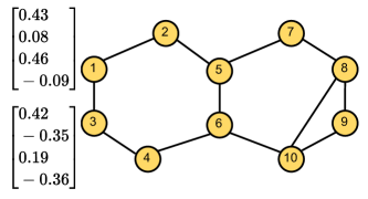
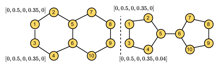
While the existing models have been applied to various domains, GNNs and graph transformers still have three inherent limitations. First, graph transformer models lack the power to capture similarity between local structures. Some recent graph transformers (e.g., GT [2] and SAN [5]) use graph structural features (e.g., Laplacian Eigenvectors) as positional encodings (PEs) to distinguish isomorphic substructures. However, although the PEs can assign distinguishable representations to substructures of individual nodes, they do not always reflect structural similarity between the substructures. PEs that account for substructure similarity are significant for the models to understand connectivity between neighbours, rather than simply aggregating their feature vectors. In Figure 1, we assign the PEs to two nodes, ‘1’ and ‘3’, with Laplacian Eigenvectors. Then, their vector representations are dissimilar, although they have similar local structures. This impreciseness can be a serious obstacle to learning representations of graph structures and eventually affect the models’ performance.

Second, GNN aggregators and self-attention lack the power to learn global structural features. GNN variants, like GCN [1], GAT [6], and GATv2 [7, 8, 9], compose node embeddings based only on features of neighbours. Similarly, graph transformer models learn node representations by encoding features of node pairs and substructures within $k$-hop distance using self-attention [10, 11, 12]. Although graph transformers have larger aggregation ranges in a layer than GNNs, neighbourhood aggregation is not powerful enough to reveal long-range dependencies or role-based similarities of nodes.

Third, the existing models lack the ability to integrate local and global structural features into a unified representation, which could benefit various downstream tasks. For example, influential nodes in social networks will be centres of different communities, and we consider both ‘influence (global)’ and ‘community (local)’ to analyse the nodes. Some GNNs and graph transformers, such as LSPE [13] and GPS [14], try to capture higher-order substructures surrounding nodes within $k$-hop distance and consider them in messages or node features. However, we cannot increase the $k$-hop distance as the graph diameter increases. Furthermore, global structural features (e.g., long-range dependencies) correlate with node roles (i.e., substructures rooted in nodes). Similar roles of nodes do not always indicate their adjacency or similar node features but rather the opposite. Therefore, the different views of the features are a significant barrier to integrating these features into a unified vector representation.

To overcome the limitations, we propose Unified Graph Transformer Networks (UGT), which can represent both local and global structural features of graphs with a unified vector representation. We first construct virtual edges connecting the distant nodes with role-based similarity. By sampling $k$-hop neighbourhoods with both virtual and actual edges, UGT can observe long-range dependencies of nodes along with their local connectivities. We propose structural identity, which is a substructure descriptor, and use it for identity mapping in transformer layers to preserve information about roles of nodes. Structural distances estimated based on the substructure descriptor are also used to compute attention scores to consider role-based similarity. Transition probabilities are used together to calculate the attention scores to consider proximity and role jointly. Finally, to bridge the gap between local and global structures, UGT is pre-trained to preserve $p$-step transition probabilities, considering all the paths between two nodes and reflecting proximity and surrounding structure in multiple scales. Our contributions are as follows:

• We propose Unified Graph Transformer Networks (UGT), which can learn local and global structural features and integrate them into a unified representation.

• Our novel sampling method constructs virtual edges between nodes with high role-based similarity and samples $k$-hop neighbourhoods to observe long-range dependencies and local connectivity together.

• The pre-training task is proposed to bridge the conceptual gap between local and global structures by preserving transition probabilities between nodes, which reflect both connectivity and surrounding structures of the nodes from all the paths connecting them, at multiple scales.

• We experimentally validated that UGT achieves comparable expressive power to the third-order Weisfeiler-Lehman isomorphism test (3d-WL) in distinguishing non-isomorphic graph pairs.

2 Related Work

This section discusses how the existing studies attempted to overcome the limitations discussed in the previous section. Several existing graph transformers attempt to reveal similarity of local structures between neighbouring nodes using PEs. SAN [5] uses learnable PEs combined with the attention mechanism to learn the local structures. Graphformer [15] adds node degree to node features and integrates edge features using shortest-path distance attention bias. GPS [14] uses random walk positional encoding (RWPE) to find similar substructures for each target node. SAT [10] extracts $k$-hop subgraph representations for each target node and uses GNNs to update the target node representations. The existing models try to consider similarity of local structures using substructures or paths surrounding nodes without preserving distances between target and context nodes, although close neighbours usually have higher significance than distant ones [16, 17]. The main difference between the existing studies and UGT is that we describe and consider substructures while preserving the distances using the structural identity and distance. By describing the distances, the structural identity goes beyond local structure descriptors to cover global structures, including the roles of nodes.

Several existing studies attempted to capture global structural features. WRGAT [18] aims to break the limitations of GNNs by using multiple relations between nodes. GeoGCNs [19] employ multiple embedding methods, such as Poincare and Struc2vec, and choose an optimal latent space that can preserve the global structural features. While the GNN variants show the capability to capture global information, they mostly overlook substructure similarity. Several graph transformers, such as SAT [10] and Graphformer [15], attempt to capture higher-order structures within $k$-hop distance [20]. However, the higher-order structures are extracted within $k$-hop distance and omit long-range dependencies since the $k$-hop distance is difficult to be extended to graph diameters. Otherwise, UGT constructs virtual edges to connect distant nodes with substructure similarity. By observing occurrences of substructures all over the graph with virtual edges and co-occurrences of substructures within $k$-hop distance with actual edges, UGT can learn both local and global structures. Then, the transition probabilities are the medium for fusing the two features.

3 Unified Graph Transformer Networks

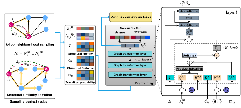
This section introduces a novel graph transformer model, UGT, which can learn local and global structural features and integrate them into a unified vector representation. We first introduce how to sample context nodes and then describe the design of UGT in detail. Finally, we introduce self-supervised learning and fine-tuning tasks. The overall architecture of UGT is described in Figure 2.

Figure 2: The overall architecture of UGT. UGT is composed of main blocks, including sampling context nodes, building modules $I$, $d$, and $m$, and pre-training blocks. The learned representations then could be used for various downstream tasks.

3.1 Sampling Context Nodes

Figure 3: An example of UGT sampling strategy. We sample context nodes within $k$-hop neighbourhoods and virtual connections between distant nodes with structural similarity.

Given a graph $G=(V,E)$ with node set $V$ and edge set $E$, we aim to sample the context node $v_j$ of each target node $v_i\in V$. The context node $v_j$ could be sampled if the distance from $v_i$ to $v_j$ within $k$-hop, or both two nodes $v_i$ and $v_j$ are structurally similar. Formally, for each target node $v_i$, the set of neighbours of $v_i$ can be defined as:

$N_i$ $=$ $N_i^{(k)}\cup N_i^{(st)},$ (1)

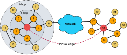
where $N_i^{(k)}$ indicates the set of neighbours of $v_i$ within $k$-hop distance, and $N_i^{(st)}$ refers to the set of nodes that are structurally similar to $v_i$. Figure 3 presents a simplified graph that contains a target node ‘1’ and its context. For global sampling, we construct virtual edges between any two nodes if they are structurally similar. For example, nodes ‘1’ and ‘12’ are structurally similar with the same degree of five and connected to two triangles. Note that we only consider similarity based on the graph structure without using the node feature. Let $I_k(v_i)$ denotes the set of an ordered degree sequence of $v_i$ in $1$ to $k$-hop. Note that $I_0(v_i)$ is the degree of $v_i$. By comparing the ordered degree sequences between $v_i$ and $v_j$, we can impose a score to measure structural distance. Formally, the structural distance and score between any two nodes $v_i$ and $v_j$ in a graph could be defined as:

$s_k=f_k(I_k(v_i),I_k(v_j)),$ (2)

$S(v_i,v_j)=\exp \left(-\sqrt{s_k}\right),$ (3)

where $f_k(\cdot ,\cdot )$ is the structural distance between two sequences. Similar to Struc2vec [21], we use dynamic time warping (DTW) to measure the distance between two ordered degree sequences. In most real-world networks, however, the degree distribution is highly asymmetric and shows a long tail distribution. To boost the connections between nodes with high degrees, we introduce another score:

$S(v_i,v_j)=\exp \left(-\sqrt{s_k}\right)+\exp \left(-{\displaystyle \frac{1}{{}^{\sqrt{\left(d_{v_i}+d_{v_j}\right)}}}}\right),$ (4)

where $d_{v_i}$ presents the degree of $v_i$. Accordingly, two nodes with a high score are structurally similar, and if they have high degrees together, they are closer in the latent space.

3.2 Learning Unified Representations of Graphs

3.2.1 Input representation

Given a graph $G$, the node feature $x_i\in R^{d_0\times 1}$ of node $v_i$ is mapped via a linear projection to $d$-dimensional hidden feature ${\widehat{x}}_i^0$, as:

${\widehat{x}}_i^0$ $=$ $W_0{x}_i+b_0,$ (5)

where $W_0\in R^{d\times d_0}$ and $b_0\in R^d$ are the parameters of the linear projection, $d_0$ refers to the original feature of $v_i$. Since we aim to make UGT can learn the global positional information context for each node in the whole graph, we add a linearly transformed positional embedding ${\lambda }_i$ of dim $k$ to node features, as:

${\widehat{\lambda }}_i$ $=$ $W_1{\lambda }_i+b_1,$ (6)

$h_i^0$ $=$ ${\widehat{x}}_i^0+{\widehat{\lambda }}_i,$ (7)

where $W_1\in R^{d\times k}$ and $b_1\in R^d$. Note that the positional embeddings are pre-calculated and added only for the first time, and we use Eigenvectors of the graph Laplacian matrix. Furthermore, we randomly flip $\lambda$ during training to allow UGT to capture sign invariance.

3.2.2 Global structural self-attention

We now propose a self-attention bias to encode local and global structural information. Since we aim to capture context nodes within a $k$-hop distance and distant nodes, the self-attention needs to understand the distance between node pairs in terms of $k$-hop distance and the structural distance. Formally, we define a self-attention between $v_i$ and $v_j$ for head $k$ at layer $l$ as:

${\alpha }_{ij}^{k,l}={\displaystyle \frac{\left(Q^{k,l}{h}_i^l\right)\cdot \left(K^{k,l}{h}_j^l\right)}{\sqrt{d_k}}}+D_{ij}^{k,l}+M_{ij}^{k,l},$ (8)

where $Q^{k,l}$, $K^{k,l}$ $\in R^{d_k\times d}$, $k=1$ to $H$ refers to the number of attention heads, $h_i$ and $h_j$ are the features of node $v_i$ and $v_j$, respectively. $D_{ij}^{k,l}$ and $M_{ij}^{k,l}$ $\in R^{d_k\times d}$ are linear transformed structural distance $d_{ij}$ and transition probability $m_{ij}$ between two nodes $v_i$ and $v_j$, respectively. We now introduce strategies to construct $d$ and $m$.

We define the structural identity of each target node based on hierarchical role-based information, including minimum, maximum, mean, and standard deviation degrees up to $k$-hop distance context of each node $v_i$. Formally, the structural identity of node $v_i$ and the structural distance could be defined as:

$I_i=\{d_{v_i},T_1,T_2,\mathrm{\cdots },T_k\},$ (9)

$d_{ij}=f\left({\left[{\Vert I_i^{(q)}-I_j^{(q)}\Vert }_2\right]}^{-1}\right),$ (10)

where $d_{v_i}$ denotes the degree of node $v_i$, $T_k=\{{\min }_k,{\max }_k,{\mu }_k,{\delta }_k\}$ denotes the set of minimum, maximum, mean, and standard deviation values of the node degrees at $k$-th hop distance, $I_i^{(q)}$ refers to the $q$-th element of $I_i$, and $f$ refers to a linearly transformed structural distance.

While structural distance can benefit the model by finding distant nodes with structural similarity, it cannot capture paths between the two nodes. To fill this gap, we present the transition probability-based distance $m$, which is the awareness of connectivity between any two nodes from a probabilistic perspective. In this way, UGT could capture both the local and global structural information, leading to the power to capture any path between nodes. We define the transition probability distance $m$ from $v_i$ to $v_j$ as:

$m_{ij}=f(A_{ij}^1,A_{ij}^2,\mathrm{\cdots },A_{ij}^p),$ (11)

where $A_{ij}^p$ refers to the transition probability from $v_i$ to $v_j$ at $p$-step, and $f$ refers to a linearly transformed transition probability.

3.2.3 Graph transformer layers

The outputs of self-attention are then concatenated into one vector representation followed by a linear transformation. The node features of $v_i$ are updated at layer $l$ as:

$${\widehat{h}}_i^{l+1}=O_h^l\underset{k=1}{\overset{𝐻}{\parallel }}\left(\sum _{v_j\in N(v_i)}{\tilde{\alpha }}_{ij}^{k,l}{V}^{k,l}{h}_j^l\right),$$ (12)

where ${\tilde{\alpha }}_{ij}^{k,l}={\text{softmax}}_j({\alpha }_{ij}^{k,l})$, $Q^{k,l}$, $K^{k,l}$,$V^{k,l}$ $\in R^{d_k\times d}$, $O_h^l\in R^{d\times d}$, and $\parallel$ refers to concatenation. The outputs then are passed to feed-forward networks (FFN) along with residual connections and layer normalization:

${\widehat{h}}_i^{l+1}=\text{LN}\left(h_i^l+{\widehat{h}}_i^{l+1}\right),$ (13)

${\widehat{\widehat{h}}}_i^{l+1}=W_2^l\text{ReLU}\left(W_1^l{\widehat{h}}_i^{l+1}\right),$ (14)

$h_i^{l+1}=\text{LN}\left({\widehat{h}}_i^{l+1}+{\widehat{\widehat{h}}}_i^{l+1}\right),$ (15)

where $W_1^l\in R^{2d\times d}$ and $W_2^l\in R^{d\times 2d}$ are learnable parameters, and LN refers to layer normalization.

Since the structural identity of nodes could sufficiently extract information around nodes based on degree information, it could benefit to distinguish non-isomorphic substructures. Therefore, we add a linearly transformed structural identity to each transformer layer, as given by Equation (12):

${\widehat{h}}_i^{l+1}=f\left(I_i^l\right)+{\widehat{h}}_i^{l+1}.$ (16)

We believe that with a number of adequate transformer layers, UGT could map different substructures into different representations.

3.3 Self-supervised Learning Tasks

We now present self-supervised learning tasks that could train UGT on pretext tasks to extract graph structure without using any label information. Our objective is to learn representations that could capture both local and global structures between any nodes as long as they are structurally similar. As mentioned earlier, we aim to preserve relational structure information in $p$-step transition probability, combining local and global structures. The learned representations could then be used for solving different downstream tasks.

Given a connectivity between a target node $v_i$ and a context node $v_j$, we aim to maximize the transition probability of paths connecting $v_i$ and $v_j$ against the probability of other pairs not from the graph. Similar to Grarep and Glove, we employ noise contrastive estimation, introduced by [22]. The loss function for the transition probability matrix of $v_i$ at $p$-step could be defined as:

$L_1^p(v_i)=\left({\displaystyle \sum _{v_j}}{P}_k\left(v_j|v_i\right)\log \sigma \left(z_i{z}_j\right)\right)+\lambda 𝔼,$ (17)

where $𝔼=E_{v_k\sim P_k(V)}\left[\log \sigma \left(-z_i{z}_k\right)\right]$, $v_k$ refers to nodes obtained from negative sampling. We then assume the noise follows a uniform distribution, and this lead to a new transition matrix on a log scale that represents precisely the global relation information between any two nodes at step $p$:

$A^{\prime (p)}=\log \left({\displaystyle \frac{A_{i,j}^{(p)}}{{\sum }_t{A}_{t,j}^{(p)}}}\right)-\log \left({\displaystyle \frac{\left|N_s\right|}{\left|V\right|}}\right),$ (18)

where $A^{\prime (p)}$ is the log scale probability matrix at step $p$ that we aim to preserve, and $N_s$ refers to the set of negative samples. Finally, the loss function for structure preservation at step $p$ can be computed as:

$L_1^p=\parallel A^{{}_{}{}^{\prime }(p)}-Z^{(p)})\parallel {}_F{}^2,$ (19)

where $Z^{(p)}$ is the score matrix that could be built by computing the cosine similarity between vector embeddings.

Since node feature information could benefit several downstream tasks, UGT should also learn a reconstruction of node feature information. We define the node raw feature reconstruction-based loss term as:

$L_2={\displaystyle \frac{1}{\left|V\right|}}{\displaystyle {\sum }_{v_i\in V}}{\Vert x_i-{\widehat{x}}_i\Vert }_2,$ (20)

where $x_i$ refers to the raw feature of node $v_i$, and $\widehat{x_i}=FFN(z_i)$. We train the model in multi-task learning with the two losses, and the losses are linearly combined as:

$L=\alpha {\displaystyle \sum _p}{L}_1^p+\beta L_2,$ (21)

where $\alpha$ and $\beta$ are hyper-parameters.

3.4 Fine-tuning Tasks

To apply UGT to downstream tasks, the learned representations are then passed directly to solve downstream tasks. In this study, we present three downstream tasks, including node clustering, node classification, and graph-level classification. For the node clustering task, we used modularity as the loss function as with [23]. For the node classification, a representation of node $v_i$ from the transformer layers was passed to fully-connected (FC) layers to get the classification output $y_i$ as:

$y_i=W_1\text{ReLU}\left(W_2{h}_i^l\right),$ (22)

where $W_1\in R^{d\times C}$ and $W_2\in R^{d\times d}$ are weight matrixes, and $C$ refers to the number of classes. In the graph-level classification, we employed average pooling to obtain graph features and likewise used FC layers to obtain the prediction output.

4 Experiments

We conducted experiments to evaluate UGT versus GNN variants and graph transformer models for three tasks: node clustering, node classification, and graph-level classification. We also analyzed the power of our model by assessing UGT on isomorphism testing.

4.1 Experimental Settings

4.1.1 Datasets

For the node-level tasks, we used eleven publicly available datasets, which are grouped into three different domains, including Air-traffic networks (e.g., Brazil, Europe, and USA) [21], Webpage networks (e.g., Chameleon, Squirrel, Actor, Cornell, Texas, and Wisconsin) [19], and Citation networks (e.g., Cora and Citeseer) [24]. We used four publicly available datasets for the graph classification task, including Enzymes, Proteins, NCI1, and NCI9 from TUDataset [25]. Furthermore, we used Graph8c and nine Strongly Regular Graphs datasets (SRGs), which contain 1d-WL and 3d-WL equivalent graph pairs, respectively, for isomorphism testing [26].

4.1.2 Baselines

The GNN variants included GCN [1], GCNII [27], GIN [28], GAT [6], GATv2 [7], SAGE [29], Geom-S [19], WRGAT [18], and DeeperGCN [30]. Furthermore, we compared UGT against recent transformers, including GT [2], SAN [5], SAT [10], GPS [14], ANS-GT [31], and Graphormer [15]. For isomorphism testing, we compare UGT against recent powerful models, i.e., ChebNet [32], and GNNML3 [26].

4.1.3 Implementation Details

We conducted each experiment ten times by randomly sampling training, validation, and testing sets of size 80%, 10%, and 10%, respectively. The results written in the tables were measured with means and standard deviation on the testing set over the ten cases. The experiments were done in two servers with four NVIDIA RTX A5000 GPUs (24GB RAM/GPU). The hyper-parameters were tuned on the validation sets for each task and dataset. For fair comparisons with the baselines, we conducted a search for the number of layers and the hidden dimension size with ranges of {2, 4, 8} and {32, 64, 128} with every model, respectively.

Brazil Europe USA Chameleon Squirrel Film Cornell Texas Wisconsin Cora Citeseer C$\downarrow$ Q$\uparrow$ C$\downarrow$ Q$\uparrow$ C$\downarrow$ Q$\uparrow$ C$\downarrow$ Q$\uparrow$ C$\downarrow$ Q$\uparrow$ C$\downarrow$ Q$\uparrow$ C$\downarrow$ Q$\uparrow$ C$\downarrow$ Q$\uparrow$ C$\downarrow$ Q$\uparrow$ C$\downarrow$ Q$\uparrow$ C$\downarrow$ Q$\uparrow$ GCN 0.71 -0.01 0.71 -0.07 0.47 0.16 0.46 0.25 0.27 0.73 0.59 0.11 0.75 0.0 0.61 0.16 0.59 0.18 0.16 0.68 0.17 0.63 GCNII 0.74 -0.02 0.76 -0.03 0.59 0.11 0.56 0.2 0.72 0.27 0.66 0.06 0.78 -0.05 0.8 -0.03 0.64 0.09 0.42 0.33 0.32 0.37 GIN 0.73 -0.03 0.01 0.01 0.08 0.1 0.47 0.13 0.75 0.27 0.59 0.04 0.81 -0.1 0.9 -0.13 0.73 -0.02 0.2 0.63 0.24 0.56 GAT 0.68 -0.01 0.74 -0.05 0.69 0.03 0.66 0.09 0.77 0.25 0.71 0.02 0.85 -0.1 0.88 -0.18 0.82 -0.07 0.17 0.66 0.25 0.55 GATv2 0.54 -0.01 0.61 -0.06 0.22 0.17 0.72 0.06 0.77 0.2 0.7 0.06 0.8 -0.08 0.88 -0.13 0.72 -0.01 0.17 0.66 0.21 0.59 SAGE 0.55 -0.02 0.76 -0.06 0.68 0.04 0.77 0.03 0.75 0.25 0.72 0.0 0.9 -0.16 0.94 -0.15 0.83 -0.07 0.18 0.65 0.23 0.57 WRGAT 0.74 -0.01 0.78 -0.05 0.71 0.03 0.64 0.09 0.69 0.34 0.67 -0.0 0.86 -0.15 0.92 -0.17 0.83 -0.12 0.23 0.6 0.28 0.53 WRGCN 0.72 -0.0 0.79 -0.05 0.7 0.03 0.64 0.1 0.68 0.34 0.67 0.0 0.88 -0.16 0.92 -0.17 0.79 -0.07 0.24 0.59 0.27 0.53 DeeperGCN 0.46 0.0 0.55 -0.06 0.5 0.1 0.75 0.04 0.78 0.26 0.75 0.03 0.8 -0.07 0.88 -0.15 0.75 -0.05 0.18 0.65 0.23 0.57 GT 0.61 -0.01 0.6 -0.05 0.31 0.12 0.78 0.02 0.78 0.22 0.8 -0.01 0.87 -0.15 0.92 -0.19 0.81 -0.11 0.19 0.64 0.26 0.54 SAN 0.6 -0.04 0.66 -0.06 0.42 0.15 0.71 0.01 0.58 0.42 0.42 0.01 0.89 -0.15 0.88 -0.12 0.79 -0.04 0.23 0.61 0.25 0.55 GPS 0.7 0.03 0.7 -0.01 0.64 -0.0 0.7 0.08 0.81 0.2 0.65 0.0 0.8 -0.09 0.73 -0.05 0.78 -0.05 0.38 0.46 0.5 0.29 SAT 0.43 0.01 0.75 -0.06 0.72 -0.0 0.8 -0.08 0.64 0.35 0.73 -0.0 0.85 -0.07 0.7 0.02 0.81 -0.04 0.58 0.01 0.39 0.12 UGT(K-mean) 0.68 0.0 0.78 -0.05 0.13 0.22 0.11 0.66 0.24 0.74 0.44 0.32 0.52 0.1 0.8 -0.1 0.67 0.03 0.10 0.71 0.15 0.66 UGT 0.51 0.22 0.51 0.20 0.34 0.30 0.11 0.64 0.21 0.39 0.28 0.50 0.28 0.47 0.33 0.46 0.27 0.52 0.09 0.76 0.04 0.78

Table 1: The performance on node clustering task in terms of conductance (C) and modularity (Q) measurements. The top three are emphasized by first, second, and third.

4.2 Performance Analysis

4.2.1 Evaluation on node clustering

We first conducted an experiment on eleven benchmark datasets for the node clustering task. For the baselines, we trained the models in a supervised manner with a classification task. Then, we used learned representations as inputs for the K-means clustering algorithm. For our UGT model, we conducted clustering using both K-means and an end-to-end manner. Table 1 shows the performance of node clustering in terms of conductance (C) and modularity (Q) measurements [33]. (1) UGT outperformed all baselines that ignore either local or global structures, e.g., GCN, WRGAT, and GT. Remarkably, the performance of our learned representations combined with K-mean also showed significant performance over the benchmark datasets. We suppose that as UGT could learn local and global structure and graph density, the representations could estimate the dense relations between nodes in communities. (2) Most of the recent graph transformers, such as SAN, SAT, Graphormer, and GPS, did not capture the density and connectivity information, only concerning higher-order neighbourhoods. This indicates that learning higher-order substructures could not help the model handle local relation density and graph partitioning.

Brazil Europe USA Chameleon Squirrel Film Cornell Texas Wisconsin Cora Citeseer GCN 41.54$\pm$9.73 37.94$\pm$2.99 50.42$\pm$5.07 66.25 $\pm$1.77 50.92 $\pm$1.02 28.15$\pm$1.37 55.55$\pm$9.29 48.89$\pm$6.47 58.40$\pm$6.49 87.33$\pm$1.71 72.05$\pm$1.22 GCNII 24.35$\pm$3.62 22.78$\pm$5.37 28.29$\pm$4.19 60.07$\pm$2.44 28.30$\pm$1.63 26.03$\pm$0.77 50.92$\pm$6.54 75.00$\pm$2.26 60.67$\pm$2.49 84.22$\pm$0.74 70.22$\pm$2.25 GIN 50.76$\pm$7.84 42.56$\pm$9.67 50.75$\pm$9.77 66.87$\pm$2.72 40.53$\pm$1.16 23.21$\pm$1.13 36.66$\pm$7.53 34.44$\pm$13.78 44.00$\pm$12.64 77.25$\pm$3.35 64.09$\pm$1.95 GAT 58.46$\pm$7.84 54.35$\pm$3.40 46.38$\pm$11.41 67.84$\pm$0.8 64.76$\pm$0.72 26.21$\pm$1.44 57.77$\pm$6.66 68.88$\pm$9.02 60.00$\pm$11.02 84.29$\pm$2.02 73.43$\pm$1.21 GATv2 69.23$\pm$8.42 57.94$\pm$4.75 61.84$\pm$ 3.38 62.20$\pm$2.11 50.80$\pm$3.01 25.73$\pm$2.11 56.66$\pm$8.88 63.33$\pm$9.68 55.20$\pm$4.66 85.77$\pm$1.27 72.95$\pm$1.87 SAGE 66.15$\pm$7.84 60.16$\pm$4.59 60.00$\pm$6.60 67.92$\pm$3.83 47.42$\pm$1.07 32.57$\pm$0.91 77.77$\pm$6.08 82.22$\pm$10.18 81.60$\pm$6.49 87.77$\pm$1.49 74.69$\pm$1.89 Geom-S - - - 58.94$\pm$0.54 36.55$\pm$0.14 30.46$\pm$0.32 54.05$\pm$0.00 64.86$\pm$0.00 58.82$\pm$0.00 83.40$\pm$0.10 73.50$\pm$0.07 WRGAT 55.38$\pm$3.07 51.28$\pm$3.62 56.97$\pm$3.54 51.80$\pm$2.03 32.96$\pm$1.44 35.78$\pm$1.84 74.44$\pm$15.55 75.55$\pm$6.66 84.80$\pm$5.30 74.59$\pm$0.50 73.01$\pm$1.71 DeeperGCN 69.23$\pm$4.86 59.49$\pm$6.76 61.17$\pm$4.99 57.53$\pm$2.82 34.96$\pm$1.04 31.68$\pm$1.50 63.33$\pm$10.30 76.67$\pm$8.16 72.80$\pm$8.54 86.59$\pm$0.85 73.61$\pm$0.62 GT 63.07$\pm$11.30 62.56 $\pm$9.53 64.37 $\pm$ 2.67 65.55$\pm$2.83 49.50$\pm$ 1.59 34.55$\pm$ 1.90 70.37$\pm$ 5.24 84.44$\pm$ 7.37 82.40$\pm$5.98 86.17$\pm$ 1.96 71.58$\pm$ 2.38 SAN 61.53$\pm$10.87 63.24$\pm$5.26 35.29$\pm$3.43 64.02$\pm$2.60 46.28$\pm$2.09 32.14$\pm$0.27 79.62$\pm$2.61 85.18$\pm$9.44 82.66$\pm$1.88 84.81$\pm$1.98 73.99$\pm$2.69 GPS 52.31$\pm$8.97 46.00$\pm$5.15 42.52$\pm$3.85 42.54$\pm$3.87 34.42$\pm$2.14 35.37$\pm$2.20 45.05$\pm$7.75 30.63$\pm$1.27 62.00$\pm$9.09 62.12$\pm$1.00 51.18$\pm$3.35 SAT 66.15 $\pm$6.15 57.43$\pm$6.19 65.04$\pm$4.06 49.69$\pm$3.81 40.08$\pm$0.76 31.61$\pm$1.37 41.67$\pm$6.33 34.44$\pm$4.15 57.60$\pm$9.32 79.63$\pm$2.69 63.98$\pm$2.41 ANS-GT 46.80$\pm$5.30 31.00$\pm$3.89 46.20$\pm$3.31 54.60$\pm$1.02 35.80$\pm$1.17 39.80$\pm$0.75 59.80$\pm$2.71 63.80$\pm$5.04 85.20$\pm$2.71 88.00$\pm$0.63 75.00$\pm$0.89 Graphormer 42.00$\pm$3.2 29.80$\pm$1.17 45.80$\pm$3.66 53.80$\pm$1.17 34.60$\pm$0.80 39.20$\pm$0.75 66.20$\pm$1.47 74.00$\pm$4.86 84.00$\pm$1.26 86.40$\pm$0.49 74.60$\pm$0.80 UGT w/o PT 76.92$\pm$4.71 44.94 $\pm$4.86 64.71$\pm$3.19 60.33 $\pm$3.91 50.43 $\pm$0.81 23.63 $\pm$1.03 52.78 $\pm$6.51 63.89 $\pm$3.93 64.0 $\pm$7.21 74.63 $\pm$2.93 57.41 $\pm$1.25 UGT 80.00 $\pm$5.23 56.92 $\pm$6.36 66.22$\pm$4.55 69.78 $\pm$3.21 66.96 $\pm$2.49 36.84$\pm$0.62 70.0 $\pm$4.44 86.67 $\pm$8.31 81.6 $\pm$8.24 88.74$\pm$0.6 76.08$\pm$2.5

Table 2: The performance on node classification task (accuracy). The top three are emphasized by first, second, and third.

4.2.2 Evaluation on node classification

We show the results of the baselines and UGT on the node classification task in Table 2. (1) Our UGT model with pre-training outperformed baseline models that overlook the long-term dependencies in most datasets, i.e., GCN, GAT, GATv2, and GT. We assume that the virtual edges allowed UGT to capture the long-term dependencies between structurally similar nodes, which have analogous roles and are significant for analyzing heterophily graphs. (2) UGT showed significant improvements in homophily graphs, i.e., Cora and Citeseer, in which nodes with the same labels tend to be adjacent. This indicates that UGT could not only capture local connectivity but also distinguish similar substructures (roles).

Enzymes Proteins NCI1 NCI109 GCN 18.24$\pm$2.05 59.23$\pm$0.62 68.24$\pm$2.38 67.09 $\pm$ 3.43 SAGE 21.46$\pm$4.32 62.79$\pm$1.38 64.36$\pm$2.82 64.47$\pm$2.41 GCNII 31.46$\pm$5.31 62.53$\pm$2.41 63.27$\pm$1.38 68.12$\pm$0.54 GIN 33.64$\pm$3.52 64.14 $\pm$ 2.05 66.72$\pm$5.32 68.44$\pm$1.89 GATv2 25.17$\pm$4.42 66.85$\pm$ 2.43 61.58$\pm$1.43 64.51$\pm$2.36 DeeperGCN 25.36$\pm$4.79 61.24$\pm$3.59 55.32$\pm$3.28 55.1$\pm$2.18 GT 41.67$\pm$6.67 77.25$\pm$3.83 69.77$\pm$1.4 69.66$\pm$0.06 SAN 22.50$\pm$0.83 68.47$\pm$0.9 59.31$\pm$3.47 57.3$\pm$8.20 SAT 50.85$\pm$3.66 62.91$\pm$0.76 54.99$\pm$0.26 56.04$\pm$0.06 GPS 62.71$\pm$8.64 53.75$\pm$6.20 79.44$\pm$0.65 76.27$\pm$0.95 UGT 67.22$\pm$3.92 80.12 $\pm$0.32 77.55 $\pm$0.16 75.45$\pm$1.26

Table 3: The performance on graph classification task in terms of accuracy. The top three are emphasized by first, second, and third.

4.2.3 Evaluation on graph-level classification

Table 3 shows the performance of the models on graph-level classification. For fair comparisons, we did not use the pre-training in the graph-level tasks, since graphs in the benchmarks have small scales. UGT exhibited competitive results compared to GNN variants and graph transformers, showing the effectiveness in capturing the global structure information in the whole graphs. This indicates that UGT could capture the connectivity in each individual substructure and then map unique substructures to different representations.

Table 4: The number of graph pairs that are undistinguished in Graph8c and nine strongly regular graphs (SRGs). Since graphs in each benchmark dataset are non-isomorphic, an ideal graph representation model should not find any similar pairs. The top two are emphasized by first and second.

GRAPH8C SR16622 SR251256 SR261034 SR281264 SR291467 SR351668 SR351899 SR361446 SR401224 $\mathrm{\#}$ Graphs 11,117 2 15 10 4 41 3854 227 180 28 $\mathrm{\#}$ Comparisions 61.8M 1 105 45 6 820 7,424,731 25,651 16,110 378 Types 1-d WL 3-d WL GCN 4,196 1 105 45 6 820 7,424,731 25,651 16,110 378 GA 1,827 1 105 45 6 820 7,424,731 25,651 16,110 378 GIN 559 1 105 45 6 820 7,424,731 25,651 16,110 378 ChebNet 44 1 105 45 6 820 7,424,731 25,651 16,110 378 PPGN 0 1 105 45 6 820 7,424,731 25,651 16,110 378 GNNML3 0 1 105 45 6 820 7,424,731 25,651 16,110 378 GT 0 0 0 0 0 0 19 0 0 2 GT w/o $\lambda$ 6,157 1 105 45 6 820 7,424,731 25,651 16,110 378 SAN 5,819 1 105 45 6 820 7,424,731 25,651 16,110 378 SAT 286,360 0 91 36 3 742 6,973,038 23,899 15,066 351 GPS 0 1 105 45 6 820 7,424,731 25,651 16,110 378 GPS w/o RWPE 1,517 1 105 45 6 820 7,424,731 25,651 16,110 378 UGT w/o $\lambda$ 355 1 105 45 6 820 7,424,731 25,651 16,110 378 UGT w/o I 36,857.0 1 105 45 6 820 7,424,731 25,651 16,110 378 UGT 0 0 0 0 0 0 0 0 0 0

4.2.4 Evaluation on the power of model

a Distinguishing non-isomorphic graphs with $\lambda$.

b Distinguishing non-isomorphic graphs with RWPE.

Figure 4: Distinguishing a Decalin graph (Left) and Bi-cyclopentyl graph (Right).

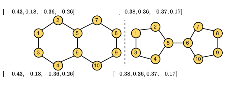
We conducted experiments to evaluate UGT on isomorphism testing for 1d-WL and 3d-WL benchmark datasets. Table 4 shows the performance on Graph8c and nine SRGs datasets. (1) UGT could perfectly distinguish non-isomorphic graph pairs in Graph8c and SRGs. Most of the GNN variants could also distinguish graphs in Graph8c. However, as GNNs’ capabilities are limited to the 1d-WL test, they failed to distinguish the graph pairs in SRGs. (2) The structural identity was effective to distinguish 1d-WL graph pairs in Graph8c, which is more powerful than $ϵ$ of GIN. Since UGT determines substructures rooted in each node through structural identity ($I$), the learned representations thus could capture the surrounding substructures of each node. (3) To investigate the reasons why UGT is more powerful than baselines, we examined differences between Laplacian Eigenvectors and RWPE. Figure 4a presents how Laplacian Eigenvectors ($\lambda$) can distinguish a decalin and bi-cyclopentyl graph pair by assigning initial PEs to nodes ‘1’ and ‘3’. At the first iteration, the input representation of UGT can be represented as $h_i^0={\widehat{x}}_i^0+W_1{\lambda }_i+b_1$ and assigns different representations from the first iteration. Thus, the output embeddings with structural identity ($h_i^{l+1}=FFN\left(I_i^l\right)+O_h^l(\cdot )$) ensure distinguishability to nodes. In contrast, RWPE needed a random walk with a length of five to distinguish the non-isomorphic graph pairs in Figure 4b. We suppose that in the SRGs, nodes are connected densely, which causes RWPE to fail to capture the substructures and connectivity in such graphs.

4.3 Ablation studies

To verify different modules in our model contribute to the overall performance, we conduct ablation studies on three benchmark datasets, including Cora, Brazil, and Cornell. Table 5 shows the results of contributions of the five models: virtual edges, I, $\lambda$, d, and m. We have the following observations: 1) Constructing virtual edges two components I and $\lambda$ could bring better performance in terms of accuracy for node classification tasks. We argue that as the Cora dataset is homophily graph, our model could understand the local and global structural information, thanks to the I and $\lambda$ components. Furthermore, UGT can also capture the long-term dependencies in Brazil and Cornell as they are heterophily graphs. This indicates that our model could effectively combine the virtual edges and two components. 2) Without virtual edges, our model can show good performance on clustering tasks. We argue that constructing virtual edges may make UGT a bit confusing the connectivity in graphs since it can affect actual edges. 4), Considering the structural distance and transition probability could contribute to the highest performance of the model in terms of accuracy for the Cora dataset. This is because the model could learn the local structural similarity and long-term dependencies even if we enable the virtual edges. For understanding local connectivity, the transition probability (m) is beneficial compared to structural distance (d). We argue that the transition probability could distinguish different connectivity between pair nodes in graphs, eventually helping the model to capture the density and the graph partitioning.

Virtual Edges I $\lambda$ Cora Brazil Cornell D M Cora Brazil Cornell acc Q C acc Q C acc Q C acc Q C acc Q C acc Q C $\mathrm{✓}$ - - 86.87 0.71 0.14 76.92 0.06 0.49 50.0 0.02 0.62 - - 85.00 0.70 0.15 76.92 0.03 0.30 50.0 0.45 0.31 $\mathrm{✓}$ - 87.06 0.73 0.12 76.92 0.09 0.52 66.67 0.21 0.43 $\mathrm{✓}$ - 86.87 0.68 0.18 84.62 0.07 0.51 55.56 0.09 0.42 - $\mathrm{✓}$ 86.50 0.72 0.13 69.23 -0.01 0.59 44.44 0.02 0.18 - $\mathrm{✓}$ 86.69 0.74 0.11 84.62 0.07 0.46 61.11 0.43 0.34 $\mathrm{✓}$ $\mathrm{✓}$ 87.80 0.70 0.15 84.62 0.03 0.20 55.56 0.24 0.29 $\mathrm{✓}$ $\mathrm{✓}$ 88.35 0.72 0.12 76.92 0.07 0.37 50.0 0.11 0.40 ✗ - - 86.32 0.70 0.15 69.23 -0.02 0.46 61.11 0.01 0.44 - - 87.61 0.73 0.12 76.92 0.02 0.13 55.56 0.55 0.23 $\mathrm{✓}$ - 87.24 0.72 0.13 84.62 0.07 0.37 66.67 0.19 0.29 $\mathrm{✓}$ - 86.50 0.73 0.12 84.62 0.03 0.20 50.0 0.17 0.45 - $\mathrm{✓}$ 87.43 0.75 0.10 76.92 0.00 0.65 50.0 0.49 0.26 - $\mathrm{✓}$ 86.32 0.73 0.12 76.92 0 0 50.0 -0.16 0.66 $\mathrm{✓}$ $\mathrm{✓}$ 85.40 0.72 0.13 84.62 0.06 0.52 55.56 0.0 0.0 $\mathrm{✓}$ $\mathrm{✓}$ 87.25 0.74 0.11 76.92 0.03 0.16 55.56 0.44 0.25

Table 5: Study the effect of virtual edges, I, $\lambda$, D, and M while keeping the other components in our model fixed. The different consequences are marked and highlighted by colours.

4.4 Sensitivity Analysis

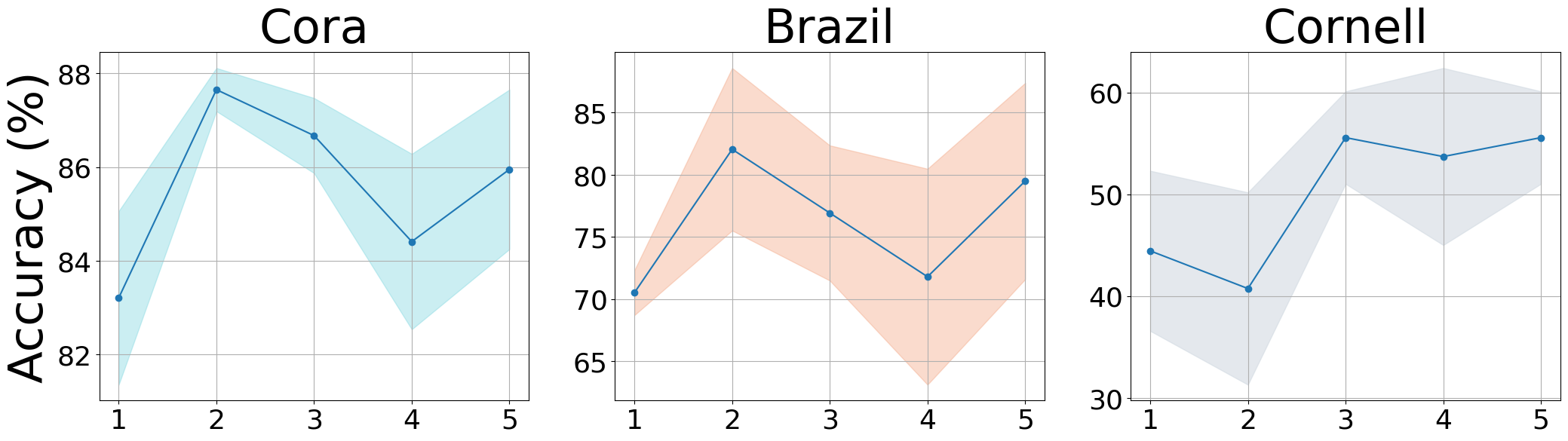
$k$-hop distance.

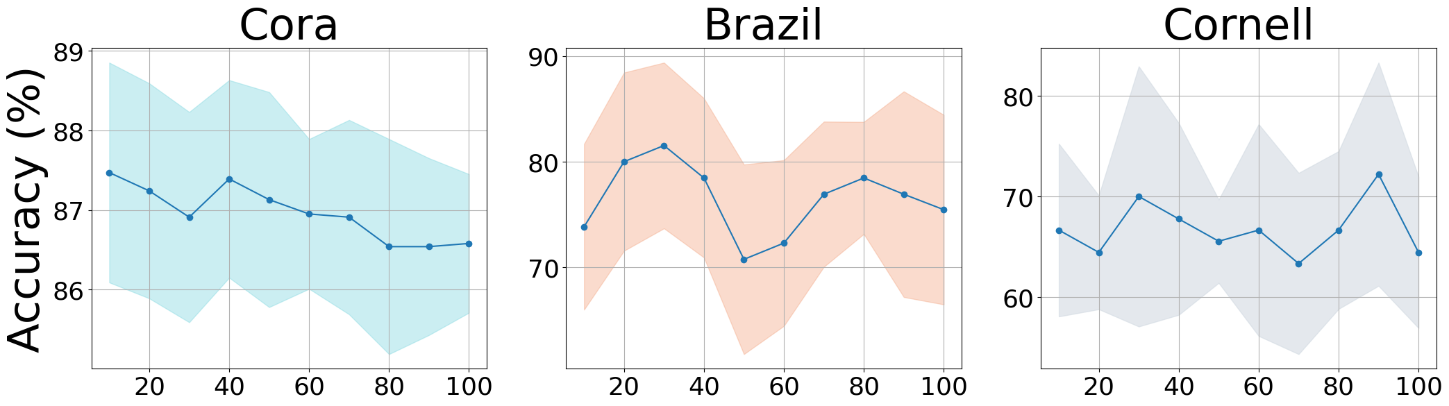
Virtual edges over actual edges.

Figure 5: The performance of node classification task according to the sampling range of context nodes up to $k$-hop distance (Above) and the percentage of virtual edges over actual edges (Below).

We performed sensitivity analyses on the range of $k$-hop neighbourhoods and the ratio of virtual edges to real edges, as shown in Figure 5. (1) As $k$ (i.e., the range of neighbourhood sampling) increased, the performance of node classification showed increasing tendencies across the three datasets. However, the trends were different for homophily and heterophily graphs. For homophily graphs (e.g., Cora), increasing $k$ up to the 3-hop range affected model performance, but not beyond. In contrast, for heterophily and sparse graphs, increasing the number of neighbourhoods provided more benefit. (2) Adding virtual edges could benefit more than increasing the number of $k$-hop neighbourhoods for the Cora dataset. We suppose that virtual edges could assist UGT in finding more distant nodes with structural similarity, and long-range dependencies could be effective for analyzing both homophily and heterophily graphs.

5 Conclusion and future work

This study proposes a novel graph transformer model, UGT, to learn local and global structural features and integrate them into a unified representation. UGT captures long-range dependencies between nodes with similar roles using structural similarity-based sampling, discovers local connectivity using $k$-hop neighbourhoods and structural identity, and unifies them by learning transition probabilities between nodes that imply both aspects. Experimental results on various downstream tasks and datasets show that UGT outperforms or is comparable to state-of-the-art GNNs and graph transformers. Since our sampling technique uses the structural similarity between nodes in the whole graph, it can cause computational complexity in large graphs. Our further research aims to reduce the computational complexity of role-based sampling by applying graph coarsening.

References

- [1] Thomas N. Kipf and Max Welling. Semi-supervised classification with graph convolutional networks. In Proceedings of the 5th International Conference on Learning Representations (ICLR 2017), Toulon, France, Apr 2017. OpenReview.net.
- [2] Vijay Prakash Dwivedi and Xavier Bresson. A generalization of transformer networks to graphs. In Proceedings of the AAAI Workshop on Deep Learning on Graphs (AAAI 2021), 8–9 Feb 2021.
- [3] Van Thuy Hoang , Hyeon-Ju Jeon , Eun-Soon You , Yoewon Yoon , Sungyeop Jung , and O-Joun Lee . Graph representation learning and its applications: A survey. Sensors, 23(8), 2023.
- [4] Hyeon-Ju Jeon, Min-Woo Choi, and O-Joun Lee. Day-ahead hourly solar irradiance forecasting based on multi-attributed spatio-temporal graph convolutional network. Sensors, 22(19):7179, 2022.
- [5] Devin Kreuzer, Dominique Beaini, William L. Hamilton, Vincent Létourneau, and Prudencio Tossou. Rethinking graph transformers with spectral attention. In Proceedings of the 34th Annual Conference on Neural Information Processing Systems (NeurIPS 2021), pages 21618–21629, Virtual Event, Dec 2021.
- [6] Petar Velickovic, Guillem Cucurull, Arantxa Casanova, Adriana Romero, Pietro Liò, and Yoshua Bengio. Graph attention networks. In Proceedings of the 6th International Conference on Learning Representations (ICLR 2018), Vancouver, BC, Canada, Apr 2018. OpenReview.net.
- [7] Shaked Brody, Uri Alon, and Eran Yahav. How attentive are graph attention networks? In Proceedings of the 10th International Conference on Learning Representations (ICLR 2022), Virtual Event, Apr 2022. OpenReview.net.
- [8] O-Joun Lee and Jason J. Jung. Story embedding: Learning distributed representations of stories based on character networks (extended abstract). In Proceedings of the 29th International Joint Conference on Artificial Intelligence (IJCAI 2020), pages 5070–5074, Yokohama, Japan, Jan 2020. ijcai.org.
- [9] O-Joun Lee, Jason J. Jung, and Jin-Taek Kim. Learning hierarchical representations of stories by using multi-layered structures in narrative multimedia. Sensors, 20(7):1978, 2020.
- [10] Dexiong Chen, Leslie O’Bray, and Karsten M. Borgwardt. Structure-aware transformer for graph representation learning. In International Conference on Machine Learning (ICML 2022), volume 162 of Proceedings of Machine Learning Research, pages 3469–3489, Baltimore, Maryland, USA, 17–23 Jul 2022. PMLR.
- [11] O-Joun Lee and Jason J. Jung. Story embedding: Learning distributed representations of stories based on character networks. Artificial Intelligence, 281:103235, 2020.
- [12] Hyeon-Ju Jeon, Gyu-Sik Choi, Se-Young Cho, Hanbin Lee, Hee Yeon Ko, Jason J Jung, O-Joun Lee, and Myeong-Yeon Yi. Learning contextual representations of citations via graph transformer. In Proceedings of the 2nd International Conference on Human-centered Artificial Intelligence (Computing4Human 2021), Da Nang, Vietnam, Oct 2021.
- [13] Vijay Prakash Dwivedi, Anh Tuan Luu, Thomas Laurent, Yoshua Bengio, and Xavier Bresson. Graph neural networks with learnable structural and positional representations. In Proceedings of the 10th International Conference on Learning Representations (ICLR 2022), Virtual Event, 25–29 Apr 2022. OpenReview.net.
- [14] Ladislav Rampásek, Michael Galkin, Vijay Prakash Dwivedi, Anh Tuan Luu, Guy Wolf, and Dominique Beaini. Recipe for a general, powerful, scalable graph transformer. In Proceedings of the 35th Annual Conference on Neural Information Processing Systems (NeurIPS 2022), 2022.
- [15] Chengxuan Ying, Tianle Cai, Shengjie Luo, Shuxin Zheng, Guolin Ke, Di He, Yanming Shen, and Tie-Yan Liu. Do transformers really perform badly for graph representation? In Proceedings of the 35th Conference on Neural Information Processing Systems (NeurIPS 2021), pages 28877–28888, Virtual Event, Dec 2021.
- [16] O-Joun Lee, Seungha Hong, and Jin-Taek Kim. Interinstitutional research team formation based on bibliographic network embedding. Mobile Information Systems, 2021:6629520:1–6629520:12, 2021.
- [17] O-Joun Lee, Hyeon-Ju Jeon, and Jason J. Jung. Learning multi-resolution representations of research patterns in bibliographic networks. Journal of Informetrics, 15(1):101126, 2021.
- [18] Susheel Suresh, Vinith Budde, Jennifer Neville, Pan Li, and Jianzhu Ma. Breaking the limit of graph neural networks by improving the assortativity of graphs with local mixing patterns. In Proceedings of the 27th Conference on Knowledge Discovery and Data Mining (KDD 2021), pages 1541–1551, Virtual Event, Aug 2021. ACM.
- [19] Hongbin Pei, Bingzhe Wei, Kevin Chen-Chuan Chang, Yu Lei, and Bo Yang. Geom-gcn: Geometric graph convolutional networks. In Proceedings of the 8th International Conference on Learning Representation (ICLR 2020), Addis Ababa, Ethiopia, 26-30 Apr 2020. OpenReview.net.
- [20] Thanh Sang Nguyen, Jooho Lee, Van Thuy Hoang, O Lee, et al. Connector 0.5: A unified framework for graph representation learning. arXiv preprint arXiv:2304.13195, 2023.
- [21] Leonardo Filipe Rodrigues Ribeiro, Pedro H. P. Saverese, and Daniel R. Figueiredo. struc2vec: Learning node representations from structural identity. In Proceedings of the 23rd International Conference on Knowledge Discovery and Data Mining (KDD 2017), pages 385–394, Halifax, NS, Canada, Aug 2017. ACM.
- [22] Michael Gutmann and Aapo Hyvärinen. Noise-contrastive estimation of unnormalized statistical models, with applications to natural image statistics. Journal of Machine Learning Research, 13:307–361, 2012.
- [23] Anton Tsitsulin, John Palowitch, Bryan Perozzi, and Emmanuel Müller. Graph clustering with graph neural networks. Journal of Machine Learning Research, 24:127:1–127:21, 2023.
- [24] Prithviraj Sen, Galileo Namata, Mustafa Bilgic, Lise Getoor, Brian Gallagher, and Tina Eliassi-Rad. Collective classification in network data. AI Magazine, 29(3):93–106, 2008.
- [25] Christopher Morris, Nils M. Kriege, Franka Bause, Kristian Kersting, Petra Mutzel, and Marion Neumann. Tudataset: A collection of benchmark datasets for learning with graphs. In Proceedings of the ICML 2020 Workshop on Graph Representation Learning and Beyond (GRL+ 2020), 2020.
- [26] Muhammet Balcilar, Pierre Héroux, Benoit Gaüzère, Pascal Vasseur, Sébastien Adam, and Paul Honeine. Breaking the limits of message passing graph neural networks. In Proceedings of the 38th International Conference on Machine Learning (ICML 2021), volume 139 of Proceedings of Machine Learning Research, pages 599–608, Virtual Event, 18–24 Jul 2021. PMLR.
- [27] Ming Chen, Zhewei Wei, Zengfeng Huang, Bolin Ding, and Yaliang Li. Simple and deep graph convolutional networks. In Proceedings of the 37th International Conference on Machine Learning (ICML 2020), volume 119 of Proceedings of Machine Learning Research, pages 1725–1735, Virtual Event, 13-18 Jul 2020. PMLR.
- [28] Keyulu Xu, Weihua Hu, Jure Leskovec, and Stefanie Jegelka. How powerful are graph neural networks? In Proceedings of the 7th International Conference on Learning Representations (ICLR 2019), New Orleans, LA, USA, May 2019. OpenReview.net.
- [29] William L. Hamilton, Zhitao Ying, and Jure Leskovec. Inductive representation learning on large graphs. In Proceedings of the 30th Annual Conference on Neural Information Processing Systems (NeurIPS 2017), pages 1024–1034, Long Beach, CA, USA, Dec 2017.
- [30] Guohao Li, Chenxin Xiong, Ali K. Thabet, and Bernard Ghanem. Deepergcn: All you need to train deeper gcns. CoRR, abs/2006.07739, 2020.
- [31] Zaixi Zhang, Qi Liu, Qingyong Hu, and Chee-Kong Lee. Hierarchical graph transformer with adaptive node sampling. In Proceedings of the 36th Annual Conference on Neural Information Processing Systems (NeurIPS 2022), New Orleans, Louisiana, 28th Nov- 9th Dec 2022.
- [32] Michaël Defferrard, Xavier Bresson, and Pierre Vandergheynst. Convolutional neural networks on graphs with fast localized spectral filtering. In Proceedings of the 29th Annual Conference on Neural Information Processing Systems (NeurIPS 2016), pages 3837–3845, Barcelona, Spain, 5–10 Dec 2016.
- [33] Jaewon Yang and Jure Leskovec. Defining and evaluating network communities based on ground-truth. Knowledge and Information Systems, 42(1):181–213, 2015.