Multimodal Industrial Anomaly Detection by Crossmodal Feature Mapping

Abstract

The paper explores the industrial multimodal Anomaly Detection (AD) task, which exploits point clouds and RGB images to localize anomalies. We introduce a novel light and fast framework that learns to map features from one modality to the other on nominal samples. At test time, anomalies are detected by pinpointing inconsistencies between observed and mapped features. Extensive experiments show that our approach achieves state-of-the-art detection and segmentation performance in both the standard and few-shot settings on the MVTec 3D-AD dataset while achieving faster inference and occupying less memory than previous multimodal AD methods. Moreover, we propose a layer-pruning technique to improve memory and time efficiency with a marginal sacrifice in performance.

1 Introduction

Industrial Anomaly Detection (AD) aims to identify unusual characteristics or defects in products, serving as a vital component within quality inspection processes. Collecting data to exemplify anomalies is challenging due to their rarity and unpredictability. Therefore, most works focus on unsupervised approaches, i.e., algorithms trained only on samples without defects, also referred to as nominal samples. Currently, most existing AD methods are geared toward analyzing RGB images. However, in many industrial settings, anomalies are hard to recognize effectively based solely on colour images, e.g., due to varying light conditions conducive to false detection and surface deviations that may not appear as unlikely colours. Deploying colour images and surface information acquired by 3D sensors can tackle the above issues and substantially improve AD.

Recently, researchers have started to explore novel avenues thanks to the introduction of benchmark datasets for 3D anomaly detection, such as MVTec 3D-AD [5] and Eyecandies [6]. Indeed, both provide RGB images alongside pixel-registered 3D information for all data samples, thereby fostering the development of new, multimodal AD approaches [42, 17, 36]. Unsupervised multimodal AD methods like BTF [17] and M3DM [42] rely on large memory banks of multimodal features. They achieve excellent performance (AUPRO@30% metric in Fig. 1) at the cost of extensive memory requirements and slow inference (Fig. 1). In particular, M3DM outperforms BTF by leveraging frozen feature extractors trained by self-supervision on large datasets, i.e., ImageNet and Shapenet, for 2D and 3D features, respectively.

Figure 1: Performance, speed and memory occupancy of Multimodal Anomaly Detection methods. The chart reports defect segmentation performance (AUPRO@30%) vs inference speed (Frame Rate on an NVIDIA 4090 GPU). The size of the symbols is proportional to memory occupancy at inference time.

Another recent multimodal method, AST [36], follows a teacher-student paradigm conducive to a faster architecture (Fig. 1). Yet, AST does not exploit the spatial structure of the 3D data but employs this information just as an additional input channel in a 2D network architecture. This results in inferior performance compared to M3DM and BTF (Fig. 1).

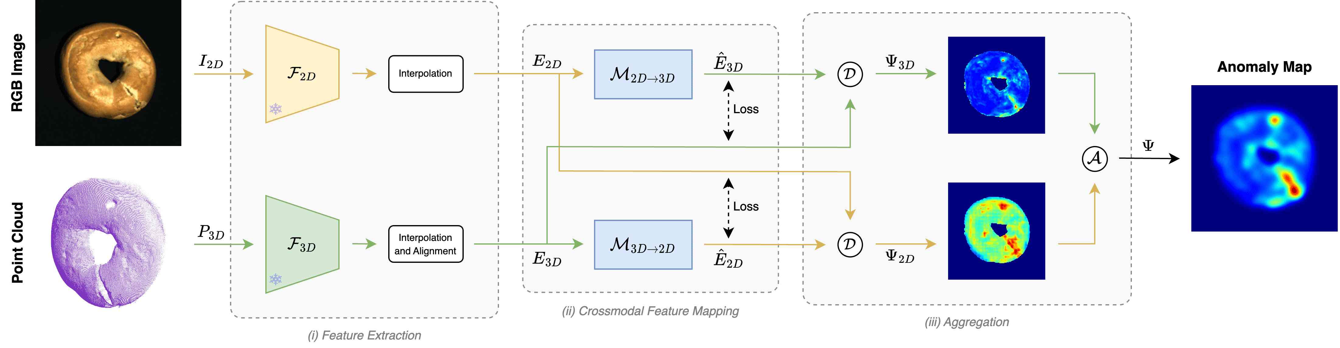
In this paper, we propose a novel paradigm to exploit the relationship between features extracted from different modalities and improve multimodal AD. The core idea behind our method, described in Fig. 2, is to learn two crossmodal mapping functions, ${ℳ}_{2D\to 3D}$ and ${ℳ}_{3D\to 2D}$, between the latent spaces of frozen 2D and 3D feature extractors, ${ℱ}_{2D}$ and ${ℱ}_{3D}$, respectively. Thus, given a 2D feature computed by the 2D extractor, ${ℳ}_{2D\to 3D}$ learns to predict the corresponding 3D feature calculated by the 3D extractor, and, likewise, ${ℳ}_{3D\to 2D}$ learns to predict a 2D feature for a given 3D feature. As we learn the two mapping functions on nominal data, we expect them to capture crossmodal relationships peculiar to good samples, while anomalies, by their quintessential nature, realize mappings unseen at training time, such as a 2D feature never observed in conjunction with a certain 3D feature, or vice versa. Hence, at inference time, we compute an anomaly map $\mathrm{\Psi }$ by estimating and aggregating the discrepancies $({\mathrm{\Psi }}_{3D},{\mathrm{\Psi }}_{2D})$ between the actual features provided by the two frozen extractors and those predicted by the crossmodal mapping functions.

This framework is amenable to realising multimodal AD effectively and efficiently. Indeed, no obvious, trivial solutions would lead the crossmodal mapping networks to generalize to defective samples. For instance, as input and output features are extracted from different modalities, the networks cannot learn identity mappings, as may have happened in previous reconstruction-based AD methods [23]. Moreover, as we will discuss in Sec. 3, modelling the relationship between 2D and 3D features in nominal data provides high sensitivity toward all kinds of anomalies. Finally, the feature mapping functions can be implemented as lightweight neural networks, such as small and shallow MLPs. This yields very fast inference alongside limited memory occupancy.

As shown in Fig. 1, our novel AD approach based on crossmodal mapping functions achieves state-of-the-art performance on MVTec 3D-AD, outperforming the best resource-intensive method based on memory banks (Ours vs M3DM), while delivering much faster inference. Additionally, we have observed that learning mappings between features from shallower layers of the frozen extractors can yield massive gains in terms of memory requirements and inference speed with a relatively limited impact on the effectiveness of our method. Thus, we can prune the deepest layers of both the 2D and 3D feature extractors to obtain Small and Tiny variants of our framework (Fig. 1: Ours-S, Ours-T) that require much less memory and run faster. Remarkably, the Small architecture still provides state-of-the-art performance on MVTec 3D-AD while requiring less than half memory compared to the full model, whereas the Tiny architecture runs almost twice as fast and outperforms BTF and AST. Finally, we point out that our method can be trained even with a few nominal samples. To properly evaluate our approach in this challenging scenario, we build the first few-shot multimodal AD benchmark from MVTec 3D-AD, and we note that our method achieves state-of-the-art anomaly segmentation performance.

Code will be released upon publication. Our contributions can be summarized as follows:

• We propose a novel framework for unsupervised multimodal AD based on mapping features across modalities;

• By using modality-specific features extracted by frozen 2D and 3D extractors, we attain state-of-the-art detection and segmentation performance on MVTec 3D-AD, while reaching performance comparable to the state-of-the-art on Eyecandies.

• Our method is capable of very fast inference and requires less memory than state-of-the-art solutions.

• We reach state-of-the-art performance on the proposed few-shot AD benchmark built on top of MVTec 3D-AD;

• We develop a strategy to prune networks without overly compromising performance. In this way, we achieve remarkably faster inference and large memory savings.

2 Related Work

Figure 2: Proposed pipeline. Given an RGB Image $I_{2D}$ and a Point Cloud $P_{3D}$: a pair of feature extractors, ${ℱ}_{2D},{ℱ}_{3D}$, extract pixel-aligned features maps, $E_{2D},E_{3D}$, by Transformer architectures. Then, a pair of crossmodal feature mappings, ${ℳ}_{2D\to 3D},{ℳ}_{3D\to 2D}$, map the extracted features from one modality to the other, processing the features at each pixel independently. Lastly, extracted, $E_{2D},E_{3D}$ and mapped, ${\widehat{E}}_{3D},{\widehat{E}}_{3D}$, features are compared through a discrepancy function $𝒟$, to create modality-specific anomaly maps, ${\mathrm{\Psi }}_{2D},{\mathrm{\Psi }}_{3D}$, that are then combined by an aggregation function, $𝒜$, to obtain the final anomaly map $\mathrm{\Psi }$.

Unsupervised Image Anomaly Detection. Unsupervised AD approaches [23] analyzing RGB Images can be divided into two broad categories. The general idea behind the first is to learn how to reconstruct images of nominal samples using auto-encoders [2, 49, 18, 33], in-painting [28], or diffusion models [43]. Then, at test time, as the trained model cannot correctly reconstruct anomalous images, a per-pixel anomaly map can be computed by analyzing the discrepancy between the input and reconstructed image. The second category of approaches focuses instead on the feature space defined by deep neural networks [31, 46, 50, 40, 47, 22, 45, 24, 48, 35, 32, 15, 10, 12]. Among these techniques, teacher-student [4, 41, 7, 38, 13] is one of the typical strategies employed for AD. During training, the teacher model extracts features from nominal samples and distils the knowledge to the student model. At test time, anomalies are detected by analysing the discrepancy between the features computed by the teacher and the student. Differently, Deep Feature Reconstruction (DFR) [44] trains an auto-encoder on the features extracted from nominal samples. Then, similarly to image reconstruction methods, it identifies anomalies in the test samples by analysing the difference between reconstructed and original features. The increasing availability of effective, general-purpose feature extractors [8, 25, 16], also referred to as foundation models, has fostered interest in anomaly detection methods that deploy features extracted by frozen models [34, 11, 1]. At training time, the features computed from nominal samples by a frozen extractor are stored in a memory bank. At inference time, the features extracted from the input image by the frozen model are compared to those stored in the bank to identify anomalies. These approaches achieve remarkable performance, albeit at the cost of slow inference — since each feature vector extracted from the input image has to be compared to all the nominal ones stored in the bank — and significant memory occupancy — since larger memory banks better capture the variability of nominal features.

Multimodal RGB-3D Anomaly Detection. Multimodal approaches exploit both RGB images and 3D data to enhance the robustness and effectiveness of anomaly detection. Following the influential work on benchmarking image-based AD [3], a recent paper [5] has introduced the MVTec 3D-AD dataset, alongside an experimental validation including several baselines, such as distribution mapping techniques based on GANs and variational models (i.e., VAEs), as well as auto-encoders. These baseline models are trained on 3D data represented by voxel grids or depth maps and incorporate RGB information as additional input channels. The method proposed in [36] consists of an asymmetric student-teacher approach (AST) aimed at processing RGB-D data, in which the two networks have different architectures to prevent over-generalization on anomalous samples. Inspired by PatchCore [34], BTF [17] investigates the use of memory banks for 3D anomaly detection. The authors propose to add 3D features to the 2D features provided by a frozen convolutional model (Wide ResNet-50) to enhance anomaly detection performance. They test several 3D features and achieve the best results using hand-crafted descriptors extracted from Point Clouds [37]. M3DM [42] improved over BTF by employing rich and distinctive 2D and 3D features extracted by frozen Transformer-based foundation models trained by self-supervision on large datasets. In particular, they use DINO [8] and Point-MAE [26] to extract 2D and 3D features, respectively. The authors also propose a learned function to fuse 2D and 3D features into multimodal features stored in memory banks alongside those computed from the individual modalities. Thanks to the joint deployment of powerful 2D, 3D and multimodal features, they achieve excellent performance, setting the highest bar on MVTec 3D-AD. However, reliance on large feature banks renders M3DM overly expensive in terms of memory and time (Fig. 1). Similarly to M3DM [42], our method deploys compelling 2D and 3D features computed by frozen Transformer-based models. Yet, we do not employ any memory bank and, instead, propose a novel crossmodal feature mapping paradigm that can be realized by two lightweight neural networks. Using the same feature extractors as M3DM [42], we achieve better performance on MVTec 3D-AD while requiring way less memory and running remarkably faster (Fig. 1).

3 Method

Our multimodal AD approach relies on learning crossmodal mappings between features extracted from nominal samples to pinpoint anomalies based on the discrepancy between predicted and observed features. As depicted in Fig. 2, this is realized by (i) a pair of frozen feature extractors ${ℱ}_{2D},{ℱ}_{3D}$; (ii) a pair of feature mappings networks ${ℳ}_{2D\to 3D},{ℳ}_{3D\to 2D}$; and (iii) an aggregation module.

3.1 Feature Extraction

The initial step in our pipeline involves extracting features for every pixel in a 2D image denoted as $I_{2D}$ and for each point in a 3D Point Cloud represented by $P_{3D}$. As explained in Sec. 1, in our framework, both feature extractors are trained on large external datasets and frozen, i.e., their weights will never be updated.

2D Feature Extraction and Interpolation. Given an image $I_{2D}$ with dimensions $H\times W\times C$ , we process it with a 2D feature extractor, denoted as ${ℱ}_{2D}$, yielding a feature map with dimensions $H_f\times W_f\times D_{2D}$. Since the dimensions $H_f$ and $W_f$ are smaller than the original $H$ and $W$, we apply a bilinear upsampling operation to obtain $E_{2D}$, which is a feature map with dimensions $H\times W\times D_{2D}$, thereby obtaining a feature vector for each pixel location.

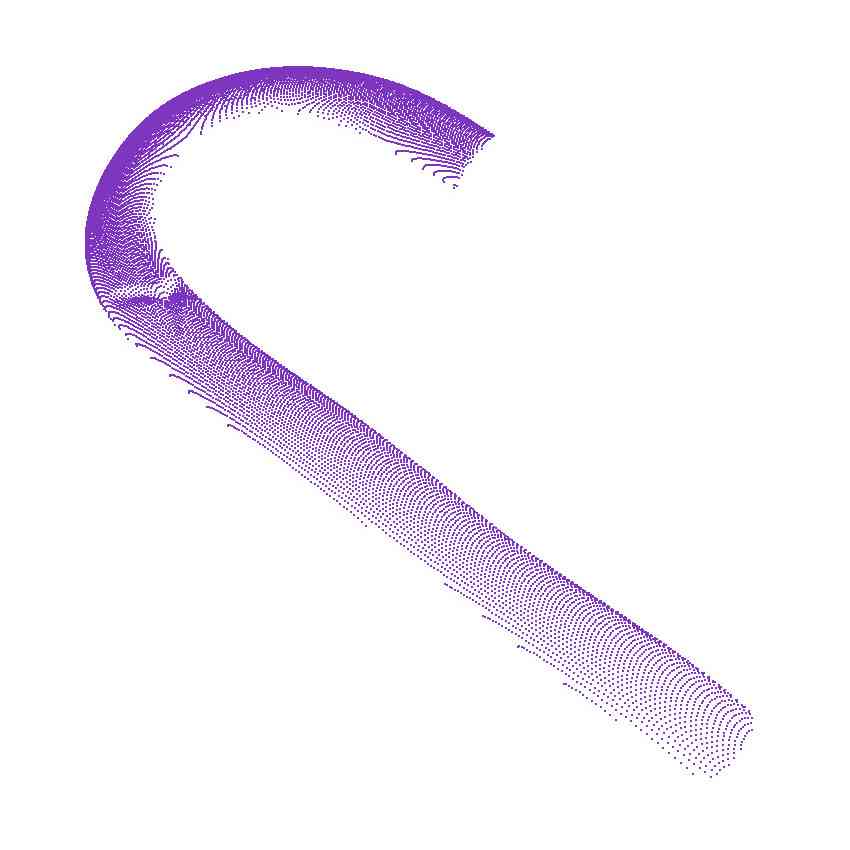
3D Feature Extraction and Interpolation. Given a point cloud of dimensions $N\times 3$, we process it with a 3D feature extractor, ${ℱ}_{3D}$, obtaining a set of $N_f$ feature vectors of size $D_{3D}$. Each feature vector, $f_{𝐜}$, is associated with a specific point within the original point cloud, $𝐜\in P_{3D}$. Indeed, many 3D feature extractors (e.g., [26]) do not estimate features for each input point but only for a subset of them, i.e., . Thus, to obtain a feature vector, $f_{𝐩}$, for each point of the cloud, $𝐩\in P_{3D}$, we follow a procedure similar to [42]. Here, $f_{𝐩}$ is computed as a weighted sum of the three feature vectors that, among the $N_f$ extracted by ${ℱ}_{3D}$, have the closest centres to $𝐩$. In this way, we obtain $E_{3D}^{\prime }$, a set of $N$ interpolated feature vectors of size $D_{3D}$.

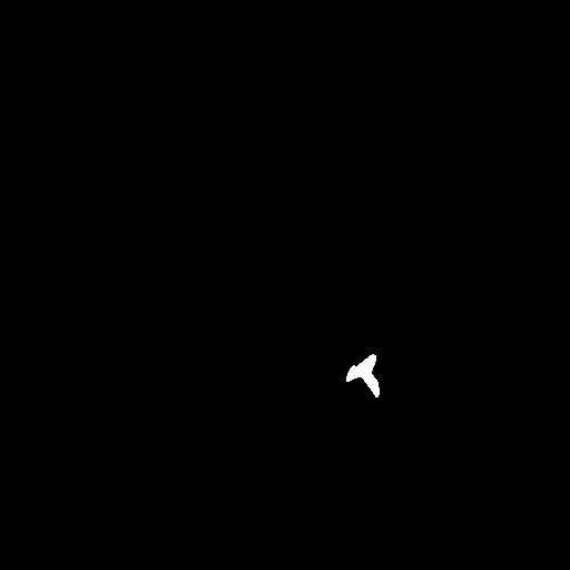
Feature Alignment. According to the standard setting in multimodal AD [5, 6], we assume pixel-registered 3D data and images. Thus, we know the corresponding pixel location associated with each 3D point. As $E_{2D}$ and $E_{3D}^{\prime }$ have been interpolated to match the original image and point cloud resolutions, we can project $E_{3D}^{\prime }$ into the 2D image plane, obtaining $E_{3D}$, a feature map of dimensions $H\times W\times D_{3D}$. In this process, we set to zero the vectors at the pixel locations where we do not have a corresponding 3D feature. Finally, we apply a $3\times 3$ smoothing kernel on $E_{3D}$. At the end of this procedure, we obtain $E_{2D}$ and $E_{3D}$, two feature maps aligned at the pixel level.

3.2 Crossmodal Feature Mapping

Once $E_{2D}$ and $E_{3D}$ have been obtained, we deploy two Feature Mapping functions, implemented as lightweight MLPs, ${ℳ}_{2D\to 3D}$ and ${ℳ}_{3D\to 2D}$. ${ℳ}_{2D\to 3D}$ maps a feature vector of size $D_{2D}$ into another one of size $D_{3D}$, while ${ℳ}_{3D\to 2D}$ does the opposite. Each network predicts features of one modality from the other, processing each pixel location independently. Thus, given a pixel location $i$, and the corresponding 2D and 3D feature, $E_{2D}^i$ and $E_{3D}^i$, we can obtain the predicted feature of the other modality as:

$${\widehat{E}}_{3D}^i={ℳ}_{2D\to 3D}(E_{2D}^i){\widehat{E}}_{2D}^i={ℳ}_{3D\to 2D}(E_{3D}^i)$$ (1)

When processing pixel locations without a 3D point associated with it, we set to zero the corresponding predicted feature. By processing all pixels, we obtain the predicted feature maps ${\widehat{E}}_{3D},{\widehat{E}}_{2D}$, of dimensions $H\times W\times D_{2D}$ and $H\times W\times D_{3D}$, respectively.

Training. At training time, ${ℳ}_{2D\to 3D}$ and ${ℳ}_{3D\to 2D}$ are jointly optimized on all the nominal samples of a dataset by minimizing the cosine distance between the feature maps computed from the input data of both modalities and the predicted ones. Thus, the per-pixel loss is:

$${ℒ}^i=\left(1-\frac{E_{2D}^i\cdot {\widehat{E}}_{2D}^i}{\Vert E_{2D}^i\Vert \Vert {\widehat{E}}_{2D}^i\Vert }\right)+\left(1-\frac{E_{3D}^i\cdot {\widehat{E}}_{3D}^i}{\Vert E_{3D}^i\Vert \Vert {\widehat{E}}_{3D}^i\Vert }\right)$$ (2)

Figure 3: Toy example of anomaly scenarios with corresponding behaviour of cross-modal mappings. Top left: Nominal samples. Top right: 2D-Only with an RGB anomaly. Bottom left: 3D-Only with an anomalous shape. Bottom right: Multimodal-Only, with nominal RGB and 3D data but anomalous correlation.

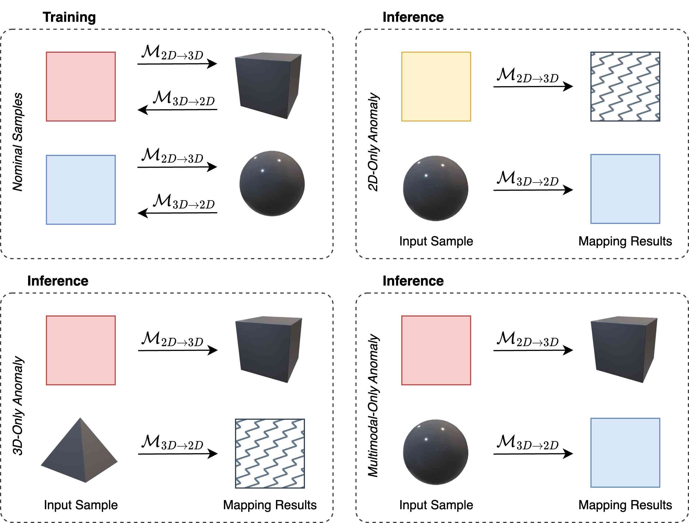
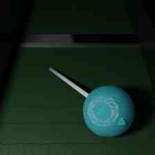
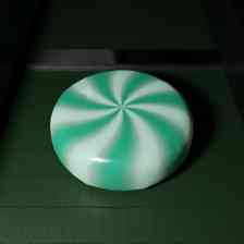
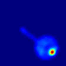
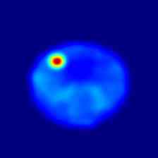
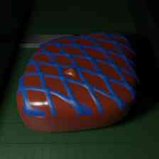
Rationale. As pointed out in Sec. 1, this novel paradigm offers high sensitivity toward all kinds of anomalies. Let us conceptualize this property with the toy examples presented in Fig. 3. At training time (top left), we observe red 2D patterns on flat 3D surfaces and blue 2D patterns on curved 3D surfaces: ${ℳ}_{2D\to 3D}$ and ${ℳ}_{3D\to 2D}$ learn to predict the relationships between the features extracted from these data. At inference time, if an anomalous, e.g., yellow, 2D pattern appears on a curved surface (top right), ${ℳ}_{3D\to 2D}$ predicts the 2D feature corresponding to a blue pattern, whilst the observed 2D feature concerns a yellow pattern. Moreover, ${ℳ}_{2D\to 3D}$ receives an input feature unseen at training time, which would unlikely yield as output the 3D feature of the actual curved surface. Thus, our method senses a discrepancy between prediction and observation for the 2D and the 3D features. Similar considerations apply to a nominal 2D pattern on an anomalous 3D surface (bottom left): both predictions disagree with the observations. This is the case also when both modalities exhibit anomalies (not shown in Fig. 3): both inputs are unseen at training time, so both crossmodal predictions are unlikely to match the observations. Finally, we highlight the case mandating multimodal AD: the individual modalities comply with the nominal distributions, but their co-occurrence is anomalous. This may be exemplified by a red pattern on a curved surface (bottom right): again, as ${ℳ}_{2D\to 3D}$ outputs the 3D feature of the flat patch and ${ℳ}_{3D\to 2D}$ the 2D feature of the blue one, both predictions disagree with the observations.

It is worth pointing out that, due to the variability of the nominal samples, the mappings between 2D and 3D features may not be unique. For instance, in Fig. 3, there might be both flat and curved surfaces coloured in red, and this one-to-many mapping makes it hard for ${ℳ}_{2D\to 3D}$ to learn the correct 3D feature to be associated to the 2D feature of a red patch. Consequently, when presented with a red patch, ${ℳ}_{2D\to 3D}$ may predict the wrong 3D feature or an unlikely one, causing a discrepancy between the predicted and observed 3D features. Yet, ${ℳ}_{3D\to 2D}$ can predict the 2D feature of the red patch, due to the $3D\to 2D$ mapping being many-to-one. Thus, we may avoid a false detection by pinpointing anomalies only when both predictions disagree with the observations. Of course, due to even higher variability across nominal samples, we may also face one-to-many $3D\to 2D$ mappings, e.g., considering again Fig. 3, both blue and red image patches on curved 3D patches. In such a case, when presented with a red patch on a curved surface, ${ℳ}_{2D\to 3D}$ may wrongly predict the feature of a flat patch and ${ℳ}_{3D\to 2D}$ that of a blue patch, ending up in a false anomaly detection due to both predictions disagreeing with the observations.

Nonetheless, in our framework, we can address the issue of potential one-to-many feature mappings across modalities by leveraging on the highly contextualized 2D and 3D features provided by Transformer architectures [8, 26]. Indeed, a contextualized 2D feature, e.g., describing a red patch surrounded by blue and purple patches, tends to correspond to a specific contextualized 3D feature, e.g., representing a flat patch just to the right of a rippling surface area. In other words, the highly contextualized 2D and 3D features extracted by Transformers are less prone to realize one-to-many crossmodal mappings. For the above reasons, we employ Transformers for both ${ℱ}_{2D}$ and ${ℱ}_{3D}$.

3.3 Aggregation

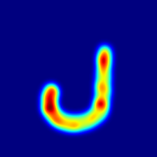
At inference time, test samples are forwarded to the Feature Extraction and Mapping networks to obtain two pairs of extracted and predicted feature maps $(E_{2D},{\widehat{E}}_{2D}),(E_{3D},{\widehat{E}}_{3D})$. After ${\mathrm{\ell }}_2$-normalization of all the individual feature vectors, the extracted and predicted maps are compared pixel-wise by a discrepancy function, $𝒟$, to obtain modality-specific anomaly maps ${\mathrm{\Psi }}_{2D},{\mathrm{\Psi }}_{3D}$:

$${\mathrm{\Psi }}_{2D}=𝒟(E_{2D},{\widehat{E}}_{2D}){\mathrm{\Psi }}_{3D}=𝒟(E_{3D},{\widehat{E}}_{3D})$$ (3)

We employ the Euclidean distance as discrepancy $𝒟$.

The above anomaly maps are then combined using an aggregation function $𝒜$ to get the final anomaly map $\mathrm{\Psi }=𝒜({\mathrm{\Psi }}_{2D},{\mathrm{\Psi }}_{3D})$. As discussed in Sec. 3.2 with the help of Fig. 3, pinpointing anomalies only when both predictions disagree with the observations provides high sensitivity across all kinds of anomalies and good robustness toward false detection. Therefore, we use the pixel-wise product as aggregation function: $\mathrm{\Psi }={\mathrm{\Psi }}_{2D}\cdot {\mathrm{\Psi }}_{3D}$, which can be thought of as a logical AND: the anomaly score at any pixel location is high only if this is so for both the modality-specific scores, i.e., anomaly detection must be corroborated by both modalities.

The aggregated anomaly map is finally smoothed by a Gaussian of kernel with $\sigma =4$, similarly to common practice [42, 34, 11]. The global anomaly score required to perform sample-level anomaly detection is obtained as the maximum value of the anomaly map $\mathrm{\Psi }$.

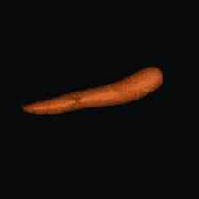
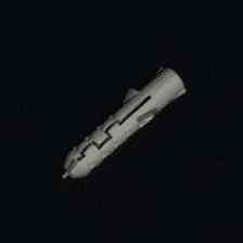
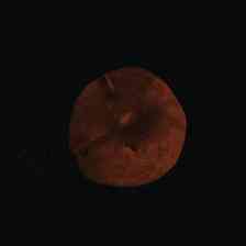
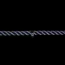
	Method	Bagel	Cable Gland	Carrot	Cookie	Dowel	Foam	Peach	Potato	Rope	Tire	Mean
I-AUROC	DepthGAN [5]	0.538	0.372	0.580	0.603	0.430	0.534	0.642	0.601	0.443	0.577	0.532
	DepthAE [5]	0.648	0.502	0.650	0.488	0.805	0.522	0.712	0.529	0.540	0.552	0.595
	DepthVM [5]	0.513	0.551	0.477	0.581	0.617	0.716	0.450	0.421	0.598	0.623	0.555
	VoxelGAN [5]	0.680	0.324	0.565	0.399	0.497	0.482	0.566	0.579	0.601	0.482	0.517
	VoxelAE [5]	0.510	0.540	0.384	0.693	0.446	0.632	0.550	0.494	0.721	0.413	0.538
	VoxelVM [5]	0.553	0.772	0.484	0.701	0.751	0.578	0.480	0.466	0.689	0.611	0.609
	BTF [17]	0.918	0.748	0.967	0.883	0.932	0.582	0.896	0.912	0.921	0.886	0.865
	AST [36]	0.983	0.873	0.976	0.971	0.932	0.885	0.974	0.981	1.000	0.797	0.937
	M3DM [42]	0.994	0.909	0.972	0.976	0.960	0.942	0.973	0.899	0.972	0.850	0.945
	Ours	0.994	0.888	0.984	0.993	0.980	0.888	0.941	0.943	0.980	0.953	0.954
AUPRO@30%	DepthGAN [5]	0.421	0.422	0.778	0.696	0.494	0.252	0.285	0.362	0.402	0.631	0.474
	DepthAE [5]	0.432	0.158	0.808	0.491	0.841	0.406	0.262	0.216	0.716	0.478	0.481
	DepthVM [5]	0.388	0.321	0.194	0.570	0.408	0.282	0.244	0.349	0.268	0.331	0.335
	VoxelGAN [5]	0.664	0.620	0.766	0.740	0.783	0.332	0.582	0.790	0.633	0.483	0.639
	VoxelAE [5]	0.467	0.750	0.808	0.550	0.765	0.473	0.721	0.918	0.019	0.170	0.564
	VoxelVM [5]	0.510	0.331	0.413	0.715	0.680	0.279	0.300	0.507	0.611	0.366	0.471
	BTF [17]	0.976	0.969	0.979	0.973	0.933	0.888	0.975	0.981	0.950	0.971	0.959
	AST [36]	0.970	0.947	0.981	0.939	0.913	0.906	0.979	0.982	0.889	0.940	0.944
	M3DM [42]	0.970	0.971	0.979	0.950	0.941	0.932	0.977	0.971	0.971	0.975	0.964
	Ours	0.979	0.972	0.982	0.945	0.950	0.968	0.980	0.982	0.975	0.981	0.971

Table 1: I-AUROC and AUPRO@30% on MVTec 3D-AD for multimodal AD methods. Best results in bold, runner-ups underlined.

Method	Bagel	Cable Gland	Carrot	Cookie	Dowel	Foam	Peach	Potato	Rope	Tire	Mean
BTF [17]	0.428	0.365	0.452	0.431	0.370	0.244	0.427	0.470	0.298	0.345	0.383
AST [36]	0.388	0.322	0.470	0.411	0.328	0.275	0.474	0.487	0.360	0.474	0.398
M3DM [42]	0.414	0.395	0.447	0.318	0.422	0.335	0.444	0.351	0.416	0.398	0.394
Ours	0.459	0.431	0.485	0.469	0.394	0.413	0.468	0.487	0.464	0.476	0.455

Table 2: AUPRO@1% on MVTec 3D-AD for multimodal AD methods. Best results in bold, runner-ups underlined.

Figure 4: Layers Pruning. The Feature Mapping networks can be fed with features from different layers of the two Transformers.

3.4 Layers Pruning

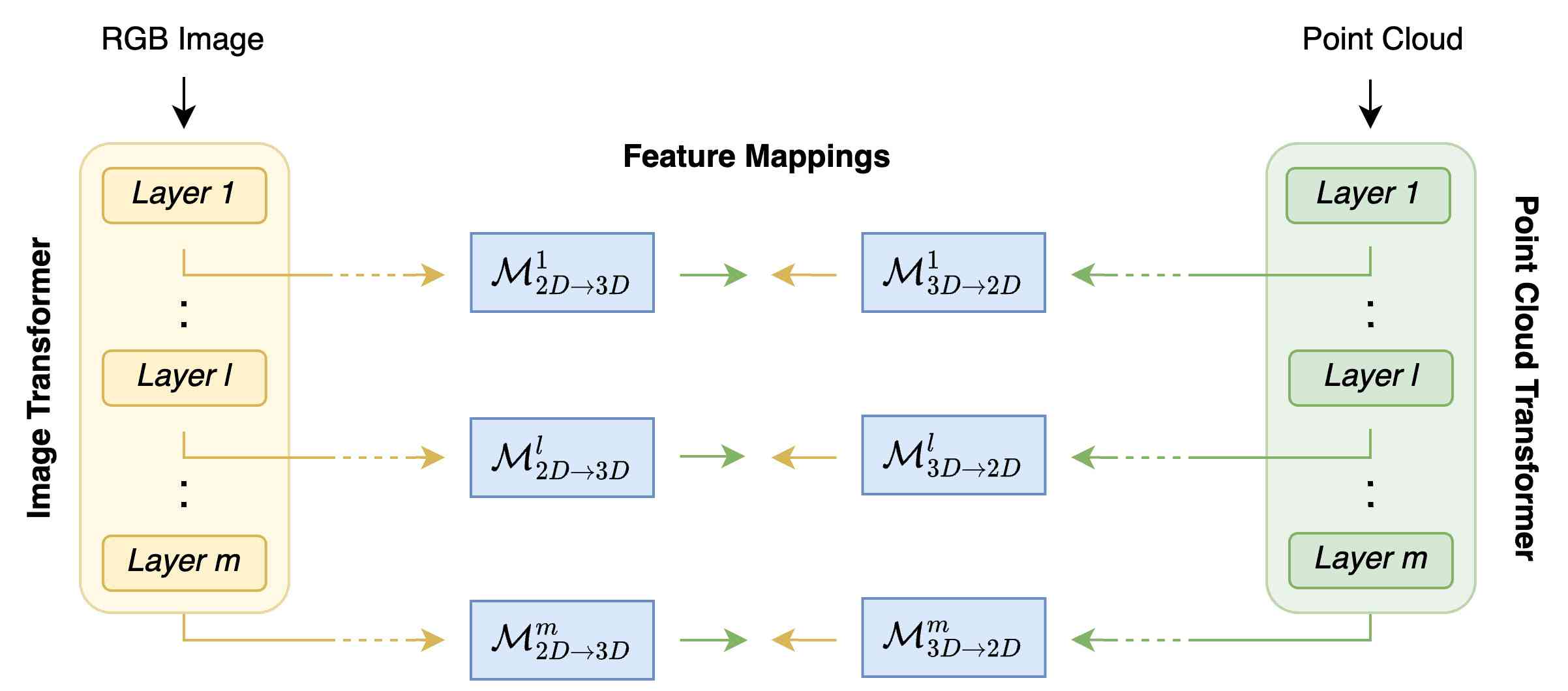
The Feature Extractors employed in our solution [8, 26] are based on Transformer encoders composed of $m$ layers. The distinguishing factor between features at different layers lies in the varying degree of self-attention processing applied to the original input. As the input features descend the encoder layers, they exhibit an increased contextualization. We observed that learning mappings between features from shallower layers of the frozen extractors can yield remarkable gains in terms of memory requirements and inference speed with a limited impact on effectiveness. Thus, as shown in Fig. 4, we prune the layers of both feature extractors at a specific layer $l$ to obtain variants which require less memory and run faster.

4 Experimental Settings

Datasets and Metrics. We evaluate our framework on two multimodal AD benchmarks. MVTec 3D-AD [5] consists of $10$ categories of industrial objects, totalling $2656$ train samples, $294$ validation samples and $1197$ test samples. Eyecandies [6] is a synthetic dataset featuring photo-realistic images of $10$ categories of food items in an industrial conveyor scenario. It contains $10k$ train samples, $1k$ validation samples and $4k$ test samples. Both datasets provide RGB images alongside pixel-registered 3D information for each sample. Thus, we have RGB information at each pixel location paired with $(x,y,z)$ coordinates. We employ the evaluation metrics proposed by MVTec 3D-AD. Thus, we assess image anomaly detection performance by the Area Under the Receiver Operator Curve (I-AUROC) computed on the global anomaly score. We estimate the anomaly segmentation performance by the pixel-level Area Under the Receiver Operator Curve (P-AUROC) and the Area Under the Per-Region Overlap (AUPRO). All previous works employ $0.3$ as the False Positive Rate (FPR) integration threshold to calculate the AUPRO. We reckon such a value may often turn out too loose for real industrial applications, allowing too many false positives. Hence, we also compute AUPRO based on the tighter $0.01$ threshold. We denote AUPROs with integration thresholds $0.3$ and $0.01$ as AUPRO@30%, and AUPRO@1%, respectively. We report results with additional thresholds in the Supplementary.

Implementation Details. We employ the same frozen Transformers as M3DM [42] to realize the ${ℱ}_{2D}$ and ${ℱ}_{3D}$ feature extractors, i.e., DINO ViT-B/8 [21, 8] trained on ImageNet [14] and Point-MAE [26] trained on ShapeNet [9], respectively. Thus, ${ℱ}_{2D}$ processes $224\times 224$ RGB images and outputs $28\times 28\times 768$ feature maps, which are bi-linearly up-sampled to $224\times 224\times 768$ before feeding the features to ${ℳ}_{2D\to 3D}$. ${ℱ}_{3D}$ processes $1024$ groups of $32$ points obtained with FPS [29], yielding a feature vector of dimensionality $1152$ for each group. As described in in Sec. 3.1, these features are interpolated and aligned to $224\times 224\times 1152$ before being fed to ${ℳ}_{3D\to 2D}$.

Both ${ℳ}_{2D\to 3D}$ and ${ℳ}_{3D\to 2D}$ consist of just three linear layers, each but the last one followed by GeLU activations. The number of units per layer is $768,960,1152$ for ${ℳ}_{2D\to 3D}$ and $1152,960,768$ for ${ℳ}_{3D\to 2D}$. The two networks are trained jointly for $250$ epochs using Adam [19] with a learning rate of $0.001$.

As done in [17, 42, 36], we fit a plane with RANSAC on the 3D point cloud and consider a point as background if the distance to the plane is less than $0.005$. Background points are discarded from the Points Clouds in input to ${ℱ}_{3D}$. This procedure accelerates the processing of 3D features during both training and inference and mitigates background noise in anomaly maps.

Moreover, as described in Sec. 3.4 to obtain lighter versions of our framework we prune both feature extractors at layer $l$ equal to $1$, $4$, $8$, to obtain Tiny, Small and Medium architectures referred to as Ours-T, Ours-S, and Ours-M.

We conducted experiments using both our and the original code from the authors of other multimodal AD methods on a single NVIDIA GeForce RTX 4090.

5 Experiments

We report here experiments to evaluate our proposal.

Method	I-AUROC	P-AUROC	AUPRO@30%	AUPRO@1%
AST [36]	0.758	0.902	0.878	0.224
M3DM [42]	0.897	0.977	0.882	0.331
Ours	0.881	0.974	0.887	0.335

Table 3: Eyecandies Results. Average metrics of 10 classes on the test set. Best results in bold, runner-ups underlined.

Method BTF [17] AST [36] M3DM [42] Ours	5-shot 10-shot 50-shot Full I-AUROC 0.671 0.695 0.806 0.865 0.680 0.689 0.794 0.937 0.822 0.845 0.907 0.945 0.811 0.845 0.906 0.954	5-shot 10-shot 50-shot Full P-AUROC 0.980 0.983 0.989 0.992 0.950 0.946 0.974 0.976 0.984 0.986 0.989 0.992 0.986 0.987 0.991 0.993	5-shot 10-shot 50-shot Full AUPRO@30% 0.920 0.928 0.947 0.959 0.903 0.835 0.929 0.944 0.937 0.943 0.955 0.964 0.949 0.954 0.965 0.971	5-shot 10-shot 50-shot Full AUPRO@1% 0.288 0.308 0.356 0.383 0.158 0.174 0.335 0.398 0.330 0.355 0.387 0.394 0.382 0.398 0.431 0.455

Table 4: Few-shot Anomaly Detection and Segmentation on the MVTec 3D-AD dataset. Best results in bold, runner-ups underlined.

	Bagel	Carrot	Dowel	Peach	Rope
RGB
PC
GT
M3DM
Ours

Figure 5: MVTec-3D AD Qualitative Results. From top to bottom: input RGB images, point clouds, GT anomaly segmentations, anomaly maps from M3DM, and anomaly maps with our method.

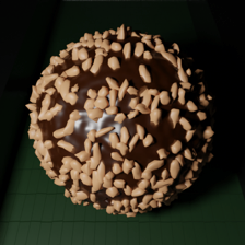
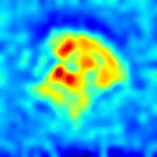
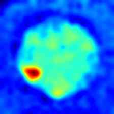
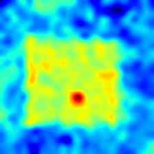
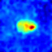
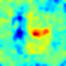
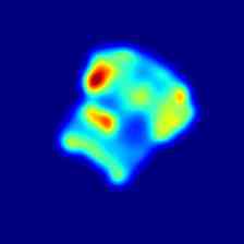
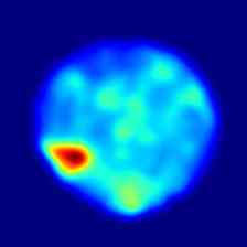
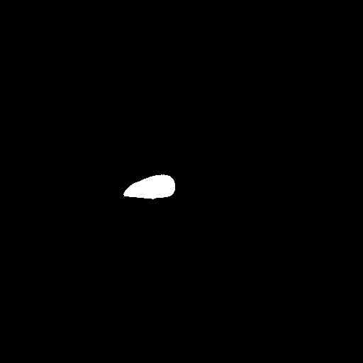
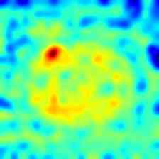
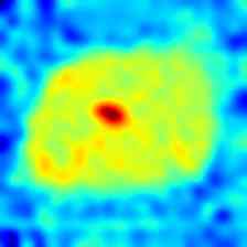
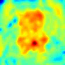
Anomaly Detection and Segmentation. Following the setups of [42], we evaluate our proposal on MVTec 3D-AD and Eyecandies, reporting results in Tab. 1, Tab. 2 and Tab. 3. Our method achieves the best results in detection and segmentation on MVTec 3D-AD, outperforming the previous state-of-the-art method, M3DM, in all the three mean metrics, namely I-AUROC, AUPRO@30% and AUPRO@1%, as well as in most of the individual categories. Comparison between Tab. 1 and Tab. 2 shows how the performance of current AD methods turn out dramatically inferior when the evaluation sets a more challenging bar in terms of tolerable FPR. As mentioned in Sec. 4, we believe that such a challenge better matches the requirements of many real industrial AD applications. Therefore, we posit that the MVTec 3D-AD benchmark is far from saturated, and there exist vast margins of improvements in multimodal AD. As for Eyecandies, Tab. 3, we achieve performance comparable to M3DM, with two winning metrics for each method. Moreover, we highlight that the P-AUROC metric seems almost saturated while also in Eyecandies there is substantial room for improvement in the AUPRO@1% metric. In Fig. 5, we show some qualitative results on the MVTec 3D-AD dataset. Compared to M3DM, our method provides remarkably sharper anomaly maps, well localized relatively to the ground-truth defect segmentation, thereby motivating the larger performance gap in terms of AUPRO@1%. More extensive qualitative results are reported in the Supplementary Material.

Method	Frame Rate	Memory	I-AUROC	P-AUROC	AUPRO@30%	AUPRO@1%
BTF [17]	3.197	381.06	0.865	0.992	0.959	0.383
AST [36]	4.966	463.94	0.937	0.976	0.944	0.398
M3DM [42]	0.514	6526.12	0.945	0.992	0.964	0.394
Ours	21.755	437.91	0.954	0.993	0.971	0.455
Ours-M	24.146	295.81	0.960	0.994	0.972	0.459
Ours-S	24.527	211.09	0.948	0.994	0.972	0.451
Ours-T	42.818	48.12	0.899	0.990	0.961	0.419

Table 5: Inference Speed, Memory Footprint and AD Performance on MVTec 3D-AD. Frame Rate in fps and Memory in MB.

Few-shot Anomaly Detection and Segmentation. In relevant industrial scenarios, collecting many nominal samples is extremely expensive or even unfeasible. Thus, a desirable property of AD methods is the ability to model the distribution of nominal data by only a few samples. To address this scenario, we define the first benchmark for few-shot multimodal AD based on the MVTec 3D-AD dataset. We randomly select 5, 10, and 50 images from each category as training data. We train the best multimodal methods, BTF [17], M3DM [42], and AST [36] on these samples, and we test them on the entire MVTec 3D-AD test set, reporting the results in Tab. 4. As for detection, our method achieves an I-AUROC comparable to M3DM [42] while outperforming the other approaches. We obtain the best segmentation performance for all metrics (P-AUROC, AUPRO@1%, and AUPRO@30%) in all the few-shot settings, significantly improving the most challenging segmentation metric (+0.052 AUPRO@1% on 5-shot). These results show that our framework enables learning general crossmodal relationships even from a few nominal samples.

Frame Rate and Memory Occupancy. Computational efficiency is key to industrial AD. Thus, we investigate the memory footprint and inference speed w.r.t. AD performance for the best multimodal approaches, BTF [17], M3DM [42], and AST [36], as well as our method. In addition, we report the performance of our framework by pruning the feature extractors at various levels using the technique described in Sec. 3.4. The results are reported in Tab. 5. We compute inference speed in frames per second on the same machine equipped with an NVIDIA 4090 and Pytorch 1.13, reporting the average across all the test samples of MVTec 3D-AD. For each method, we include the time for each step of its inference pipeline, from input pre-processing to the computation of anomaly scores, synchronizing all GPU threads before estimating the total inference time. We do not include training-only steps such as the memory bank creation. Regarding memory occupancy during inference, we consider network parameters, activations, and memory banks. As expected, memory-bank methods (BTF [17] and M3DM [42]) exhibit the lowest frame rate and the highest memory footprint. AST [36] requires only 26 MB more than our model, as it is based on two feed-forward networks. However, it is still relatively slow ($4.966$ fps) since it is based on Normalizing Flow [27]. Our method has the highest frame rate ($21.755$ fps) and the lowest memory occupancy ($437.91$ MB) while outperforming competitors across all metrics. The pruned models Ours-M, Ours-S, and Ours-T are even more efficient with a marginal sacrifice in accuracy. For instance, Ours-S occupies half of the memory of our full model and yet achieves state-of-the-art results on MVTec 3D-AD on all metrics. Remarkably, Ours-T obtains state-of-the-art anomaly segmentation performance according to the most challenging metric (AUPRO@1%=$0.419$) while running in real-time ($48.12$ fps).

Aggregation Analysis. We investigate on the impact of the proposed product-based aggregation discussed in Sec. 3.3. In Tab. 6, we report the results obtained on MVTec 3D-AD by using the anomaly maps before aggregation, ${\mathrm{\Psi }}_{2D}$ and ${\mathrm{\Psi }}_{3D}$, or combined using different functions, such as pixel-wise sum ${\mathrm{\Psi }}_{2D}+{\mathrm{\Psi }}_{3D}$, pixel-wise maximum $\max ({\mathrm{\Psi }}_{2D},{\mathrm{\Psi }}_{3D})$, and pixel-wise product ${\mathrm{\Psi }}_{2D}\cdot {\mathrm{\Psi }}_{3D}$. It is possible to note how the product performs best in both detection and segmentation. Indeed, considering as anomalous only points in which both ${\mathrm{\Psi }}_{2D}$ and ${\mathrm{\Psi }}_{3D}$ have high scores, enables discarding false positives that may occur when nominal relationships between RGB and 3D features are not unique, as discussed in Sec. 3.2.

Anomaly Map	I-AUROC	P-AUROC	AUPRO@30%	AUPRO@1%
${\mathrm{\Psi }}_{2D}$	0.895	0.985	0.950	0.401
${\mathrm{\Psi }}_{3D}$	0.885	0.987	0.956	0.403
${\mathrm{\Psi }}_{2D}$ + ${\mathrm{\Psi }}_{3D}$	0.939	0.988	0.959	0.430
$\max ({\mathrm{\Psi }}_{2D}$, ${\mathrm{\Psi }}_{3D})$	0.895	0.985	0.950	0.400
${\mathrm{\Psi }}_{2D}\cdot {\mathrm{\Psi }}_{3D}$	0.954	0.993	0.971	0.455

Table 6: Analysis of Aggregation Functions. Results on MVTec 3D-AD. Best results in bold.

Modality	Anomaly Map	I-AUROC	P-AUROC	AUPRO@30%	AUPRO@1%
Intra	${\mathrm{\Phi }}_{2D}$	0.860	0.980	0.932	0.361
Intra	${\mathrm{\Phi }}_{3D}$	0.816	0.970	0.900	0.348
Intra	${\mathrm{\Phi }}_{2D}\cdot {\mathrm{\Phi }}_{3D}$	0.898	0.989	0.963	0.426
Cross	${\mathrm{\Psi }}_{2D}$	0.865	0.982	0.944	0.382
Cross	${\mathrm{\Psi }}_{3D}$	0.885	0.985	0.952	0.391
Cross	${\mathrm{\Psi }}_{2D}\cdot {\mathrm{\Psi }}_{3D}$	0.944	0.993	0.970	0.450

Table 7: Crossmodal vs Intramodal. Results on MVTec 3D-AD. Best results in bold. Networks are trained for 50 epochs.

${ℱ}_{2D}$	I-AUROC	P-AUROC	AUPRO@30%	AUPRO@1%
DINO [8]	0.949	0.992	0.968	0.445
SAM [20]	0.792	0.973	0.906	0.311
CLIP [30]	0.833	0.984	0.942	0.346
DINO-v2 [25]	0.958	0.992	0.964	0.437

Table 8: 2D Feature Extractor Alternatives. Results on MVTec 3D-AD. Best results in bold. Networks are trained for 50 epochs.

Crossmodal Mapping vs Intramodal Reconstruction. The authors of DFR [44] argued that learning a reconstruction network in feature space from nominal samples makes it possible to detect anomalies in RGB images by analyzing the reconstruction error. As our method may be thought of as performing a Crossmodal reconstruction in feature space, we investigate the impact of learning Crossmodal vs. Intra-modal feature mapping functions. Tab. 7 compares the results of our approach (Cross) to those obtained by modifying the input layers of both our mapping networks so as to learn to reconstruct features within the same modality (Intra). The results obtained by reconstructing each modality independently show that our proposed crossmodal feature mapping sets forth a more effective modality-specific learning objective w.r.t. intra-modal feature reconstruction (rows 1 vs. 4, 2 vs. 5). This yields better results also by the aggregated maps obtained by pixel-wise product (rows 3 vs. 6).

Different 2D Feature Extractors. The ever-increasing availability of frozen Transformer-based RGB feature extractors trained on large data corpora has motivated us to explore alternatives to DINO ViT-B/8, such as, in particular, the ViT-B/16 used in SAM [20], the ViT-B/16 used in CLIP [30], and the ViT-B/14 used in DINO-v2 [25]. Results obtained on MVTec 3D-AD with the different 2D Feature Extractors are reported in Tab. 8. Interestingly, DINO and DINO-v2 exhibit much better performance than other feature extractors, which hints at - and may foster further investigation on - the benefits of foundation models trained via self-supervised contrastive learning in industrial AD.

6 Conclusions and Limitations

We have developed an effective and efficient multimodal AD framework based on the core idea of mapping features extracted by Transformer architectures across modalities. This novel paradigm outperforms previous resource-intensive methods on the MVTec 3D-AD benchmark while delivering substantially faster inference speed. Additionally, we have proposed a layer-pruning strategy for frozen Transformer encoders that can vastly reduce the memory footprint and yield even faster inference without compromising AD performance. Lastly, we also outperform competitors in the challenging few-shot scenario, achieving state-of-the-art performance on the proposed multimodal few-shot AD benchmark. A limitation of our approach lies in its multimodal-only nature, i.e., our paradigm cannot be applied to 2D AD or 3D AD, as it mandates data from both modalities at training and test times. In future work, we plan to extend our paradigm to pursue high-resolution anomaly detection by deploying coordinate-based networks, such as [39], to realize crossmodal mapping functions.

Supplementary Material

This supplementary material includes additional experimental results. In particular, we report:

• A more detailed analysis on the dynamic of the PRO (Per-Region Overlap) curve, alongside comparisons dealing with different integration thresholds;

• An ablation study concerning the architecture of the Feature Mapping networks, i.e. the core components in our method;

• Additional quantitative and qualitative results dealing with both MVTec 3D-AD and Eyecandies;

• A type correction of the main paper.

A Analysis of the PRO curve

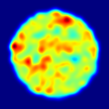
The chart in Fig. 2 reports the Per-Region Overlap curve provided by our method on class Foam of the MVTec 3D-AD dataset. The chart shows how most of the dynamic of the curve is concentrated way underneath the $0.3$ integration threshold used to define the popular AUPRO@30% metric. This is also highlighted in Fig. 2, which compares the different Multimodal AD methods focusing on lower FPRs.

Figure 1: PRO curve - Whole FPR Range. Per-Region Overlap curve obtained by our method on class Foam of MVTec 3D-AD. The dotted line shows the AUPRO@30% threshold.

Figure 2: PRO curve - Lower FPRs. Per-Region Overlap curve obtained by all Multmodal AD methods on class Foam of MVTec 3D-AD. Focus on the [0-0.3] FPR range.

Thus, as discussed in the main paper, on one hand choosing FPR=0.3 as integration threshold may not match the requirements of a number of industrial applications, on the other, it tends to wash out the performance differences between the methods, which, indeed, behave much more differently at lower, i.e., more challenging FPRs. Hence, we deem it worth considering also more demanding variants of the AUPRO metric, such as, in particular, those obtained with integration thresholds 0.1, 0.05, and 0.01, referred to as AUPRO@10%, AUPRO@5% and AUPRO@1%, respectively. As illustrated in Fig. 3, our proposal consistently provides better performance (i.e., higher AUPRO) than previous Multimodal AD methods across all the considered variants of the AUPRO metric while running much faster and requiring way less memory. In particular, the performance gap is higher for the more challenging variants of the AUPRO.

Figure 3: Performance, speed and memory occupancy of Multimodal Anomaly Detection methods. The chart reports anomaly segmentation performance on MVTec 3D-AD according to different AUPRO variants (from left to right: AUPRO@10%, AUPRO@5%, AUPRO@1% ) vs. inference speed (Frame Rate on an NVIDIA 4090 GPU). The size of the symbols is proportional to memory occupancy at inference time.

B Feature Mapping Networks

We investigate the use of alternative network architectures to implement the Feature Mapping functions, namely: (i) MLP Encoder-Decoder, (ii) MLP Projection, i.e. the architecture described in the main paper, and (iii) Convolutional Encoder-Decoder.

The MLP Encoder-Decoder architecture comprises an encoding stage and a decoding stage, each consisting of two layers, along with an extra bottleneck layer between these two stages. The input layer in the encoding stage has a number of neurons equal to the dimensionality of the input feature space, while the last layer in the decoding stage has a number of neurons equal to the dimensionality of the output feature space. Between each pair of successive layers, but for the bottleneck layer, the number of neurons is either halved (in the encoding stage) or doubled (in the decoding stage). Accordingly, in our setup, we have $[768,384,192,192,384,1152]$ neurons in each layer for ${ℳ}_{2D\to 3D}$, and $[1152,576,288,288,576,768]$ neurons in each layer for ${ℳ}_{3D\to 2D}$. In both networks, all but the last layer employ GeLU activations.

Metric	Bagel	Cable Gland	Carrot	Cookie	Dowel	Foam	Peach	Potato	Rope	Tire	Mean
	MLP Encoder-Decoder
I-AUROC	0.993	0.858	0.992	0.988	0.985	0.911	0.959	0.866	0.986	0.864	0.940
AUPRO@30%	0.979	0.959	0.982	0.940	0.946	0.960	0.980	0.982	0.972	0.981	0.968
AUPRO@10%	0.938	0.882	0.946	0.890	0.843	0.883	0.941	0.946	0.918	0.942	0.913
AUPRO@5%	0.879	0.791	0.893	0.830	0.749	0.797	0.883	0.892	0.853	0.884	0.845
AUPRO@1%	0.467	0.385	0.487	0.455	0.385	0.395	0.466	0.480	0.451	0.466	0.444
Frame Rate (fps)											25.769
Memory (MB)											369.856
	MLP Projection (main paper)
I-AUROC	0.990	0.894	0.986	0.989	0.980	0.916	0.951	0.916	0.986	0.886	0.949
AUPRO@30%	0.979	0.963	0.982	0.940	0.944	0.961	0.980	0.983	0.972	0.980	0.968
AUPRO@10%	0.937	0.892	0.947	0.890	0.838	0.885	0.940	0.948	0.918	0.941	0.914
AUPRO@5%	0.878	0.806	0.894	0.830	0.742	0.799	0.882	0.897	0.853	0.882	0.846
AUPRO@1%	0.469	0.402	0.486	0.450	0.380	0.397	0.463	0.490	0.453	0.463	0.445
Frame Rate (fps)											21.755
Memory (MB)											437.911
	Convolutional Encoder-Decoder
I-AUROC	0.997	0.866	0.990	0.993	0.989	0.927	0.979	0.897	0.990	0.918	0.955
AUPRO@30%	0.979	0.965	0.982	0.941	0.948	0.969	0.982	0.983	0.977	0.981	0.971
AUPRO@10%	0.938	0.897	0.947	0.893	0.847	0.906	0.945	0.948	0.931	0.944	0.920
AUPRO@5%	0.880	0.813	0.894	0.834	0.756	0.820	0.891	0.896	0.872	0.889	0.855
AUPRO@1%	0.469	0.409	0.488	0.453	0.393	0.409	0.477	0.488	0.467	0.473	0.453
Frame Rate (fps)											9.906
Memory (MB)											2780.690

Table 9: Results on MVTec 3D-AD, Models trained for 50 epochs. Best results in bold, runner-ups underlined.

Metric	Bagel	Cable Gland	Carrot	Cookie	Dowel	Foam	Peach	Potato	Rope	Tire	Mean
	${\mathrm{\Psi }}_{2D}$
I-AUROC	0.937	0.864	0.984	0.951	0.984	0.789	0.915	0.736	0.968	0.825	0.895
AUPRO@30%	0.960	0.966	0.979	0.884	0.911	0.916	0.981	0.974	0.958	0.971	0.950
AUPRO@10%	0.896	0.906	0.937	0.813	0.741	0.783	0.942	0.922	0.878	0.913	0.873
AUPRO@5%	0.819	0.834	0.874	0.738	0.624	0.675	0.884	0.844	0.789	0.841	0.792
AUPRO@1%	0.410	0.427	0.456	0.371	0.311	0.326	0.468	0.410	0.401	0.429	0.401
	${\mathrm{\Psi }}_{3D}$
I-AUROC	0.948	0.770	0.968	0.981	0.937	0.893	0.694	0.909	0.939	0.812	0.885
AUPRO@30%	0.967	0.922	0.981	0.926	0.919	0.965	0.965	0.981	0.963	0.976	0.956
AUPRO@10%	0.903	0.782	0.943	0.871	0.764	0.899	0.894	0.943	0.892	0.928	0.882
AUPRO@5%	0.817	0.664	0.887	0.806	0.661	0.812	0.793	0.887	0.818	0.858	0.800
AUPRO@1%	0.402	0.302	0.474	0.443	0.341	0.389	0.338	0.474	0.431	0.437	0.403
	${\mathrm{\Psi }}_{2D}+{\mathrm{\Psi }}_{3D}$
I-AUROC	0.980	0.893	0.991	0.996	0.980	0.844	0.970	0.876	0.966	0.894	0.939
AUPRO@30%	0.969	0.968	0.980	0.904	0.914	0.958	0.982	0.977	0.961	0.977	0.959
AUPRO@10%	0.917	0.912	0.941	0.853	0.749	0.877	0.945	0.932	0.886	0.931	0.894
AUPRO@5%	0.852	0.844	0.882	0.799	0.638	0.784	0.890	0.864	0.806	0.869	0.823
AUPRO@1%	0.448	0.439	0.468	0.462	0.323	0.384	0.478	0.439	0.424	0.456	0.432
	$\max ({\mathrm{\Psi }}_{2D},{\mathrm{\Psi }}_{3D}$)
I-AUROC	0.937	0.865	0.984	0.951	0.983	0.789	0.915	0.736	0.968	0.825	0.895
AUPRO@30%	0.960	0.966	0.979	0.884	0.911	0.916	0.981	0.974	0.958	0.971	0.950
AUPRO@10%	0.896	0.906	0.937	0.813	0.741	0.783	0.942	0.922	0.878	0.913	0.873
AUPRO@5%	0.819	0.834	0.874	0.738	0.624	0.675	0.884	0.844	0.789	0.841	0.792
AUPRO@1%	0.410	0.428	0.456	0.371	0.311	0.326	0.468	0.410	0.401	0.429	0.401
	${\mathrm{\Psi }}_{2D}\cdot {\mathrm{\Psi }}_{3D}$
I-AUROC	0.994	0.888	0.984	0.993	0.980	0.888	0.941	0.943	0.980	0.953	0.954
AUPRO@30%	0.979	0.972	0.982	0.945	0.950	0.968	0.980	0.982	0.975	0.981	0.971
AUPRO@10%	0.937	0.917	0.947	0.897	0.855	0.906	0.942	0.947	0.926	0.944	0.922
AUPRO@5%	0.877	0.843	0.894	0.840	0.765	0.828	0.884	0.894	0.865	0.889	0.858
AUPRO@1%	0.459	0.431	0.485	0.469	0.394	0.413	0.468	0.487	0.464	0.476	0.455

Table 10: Aggregation analysis. Best results in bold, runner-ups underlined.

As to MLP Projection architecture, we refer to shallow MLPs consisting of three layers, with GeLU activations but in the last one. The input layer has a number of neurons equal to the dimensionality of the input feature space, while the last layer has a number of neurons equal to the dimensionality of the output feature space. The intermediate layer has a number of neurons equal to the mean between the dimensionality of the input and output features. Thus, as also reported in the main paper, in our setup the three layers in ${ℳ}_{2D\to 3D}$ have $768$, $960$ and $1152$ neurons each, while the three layers of ${ℳ}_{3D\to 2D}$ have $1152$, $960$ and $768$ neurons each.

Finally, unlike the previous two architectures which ingest individual feature vectors, the Convolutional Encoder-Decoder receives input tensors of spatial size $H\times W$ (with $D_{2D}$ and $D_{3D}$ channels for ${ℳ}_{2D\to 3D}$ and ${ℳ}_{3D\to 2D}$, respectively). The architecture follows a UNet-like structure without skip-connections, with two 3x3 convolutional layers followed by 2x2 max-pooling in the encoder stage and one 3x3 conv followed by a 2x2 transpose convolution in the decoding stage. All layers except the last one employ ReLU activations. The number of channels is kept equal to the input one up to the last layer, where it is modified so as to match the dimensionality of output feature space (i.e. from $D_{2D}$ and $D_{3D}$ for ${ℳ}_{2D\to 3D}$ and from $D_{3D}$ and $D_{2D}$ for ${ℳ}_{3D\to 2D}$.

For this new set of experiments, we follow the same training protocol as defined in the main paper. The results on MVTec 3D-AD are reported in Tab. 9, and show that the Convolutional Encoder-Decoder architecture provides slightly superior performance. However, despite its enhanced performance, it operates at a significantly slower inference rate, namely $9.906$ fps, in contrast to the $21.755$ fps achieved by our base model which is based on the MLP Projection architecture. Furthermore, the Convolutional Architecture requires six times more memory compared to our base model, e.g., $2780.690$ MB compared to $437.911$ MB. Thus, we are led to prefer the performance vs efficiency (both speed and memory) trade-off provided by the MLP Projection architecture.

C Additional Quantitative Results

In this section, we report the class-wise anomaly detection and segmentation results for some of the experiments discussed in the main paper, considering also the additional FPR thresholds to compute the AUPRO introduced in Sec. A.

Metric	Bagel	Cable Gland	Carrot	Cookie	Dowel	Foam	Peach	Potato	Rope	Tire	Mean
	Ours
I-AUROC	0.994	0.888	0.984	0.993	0.980	0.888	0.941	0.943	0.980	0.953	0.954
AUPRO@30%	0.979	0.972	0.982	0.945	0.950	0.968	0.980	0.982	0.975	0.981	0.971
AUPRO@10%	0.937	0.917	0.947	0.897	0.855	0.906	0.942	0.947	0.926	0.944	0.922
AUPRO@5%	0.877	0.843	0.894	0.840	0.765	0.828	0.884	0.894	0.865	0.889	0.858
AUPRO@1%	0.459	0.431	0.485	0.469	0.394	0.413	0.468	0.487	0.464	0.476	0.455
	Ours-M
I-AUROC	0.988	0.875	0.984	0.992	0.997	0.924	0.964	0.949	0.979	0.950	0.960
AUPRO@30%	0.980	0.966	0.982	0.947	0.959	0.967	0.982	0.983	0.976	0.982	0.972
AUPRO@10%	0.941	0.901	0.947	0.899	0.880	0.901	0.945	0.949	0.930	0.947	0.924
AUPRO@5%	0.884	0.817	0.895	0.842	0.798	0.823	0.890	0.898	0.872	0.893	0.861
AUPRO@1%	0.480	0.398	0.490	0.467	0.413	0.408	0.481	0.494	0.468	0.488	0.459
	Ours-S
I-AUROC	0.983	0.878	0.973	0.992	0.987	0.913	0.900	0.936	0.981	0.941	0.948
AUPRO@30%	0.978	0.960	0.982	0.948	0.960	0.972	0.977	0.983	0.976	0.981	0.972
AUPRO@10%	0.936	0.882	0.947	0.900	0.884	0.918	0.932	0.949	0.929	0.943	0.922
AUPRO@5%	0.874	0.782	0.894	0.843	0.800	0.845	0.864	0.898	0.870	0.886	0.856
AUPRO@1%	0.461	0.379	0.492	0.479	0.411	0.429	0.430	0.494	0.467	0.472	0.451
	Ours-T
I-AUROC	0.948	0.784	0.946	0.985	0.946	0.855	0.815	0.932	0.989	0.794	0.899
AUPRO@30%	0.977	0.903	0.981	0.950	0.945	0.956	0.973	0.983	0.973	0.973	0.961
AUPRO@10%	0.932	0.736	0.944	0.901	0.838	0.873	0.919	0.949	0.920	0.918	0.893
AUPRO@5%	0.867	0.612	0.889	0.844	0.729	0.773	0.839	0.897	0.856	0.838	0.814
AUPRO@1%	0.449	0.267	0.487	0.487	0.364	0.369	0.395	0.491	0.462	0.421	0.419

Table 11: Layers Pruning analysis. Best results in bold, runner-ups underlined.

In particular, Tab. 10 provides a detailed view of the results for the Aggregation function introduced in Sec. 3.3 of the main paper. As already highlighted in the evaluation summarized in Tab. 6 and discussed in Sec. 5 of the main paper, the product aggregation achieves the best results across most of the classes except for one class, i.e., Peach, which shows higher results using the sum aggregation. These results further support our choice of relying on the product function, which realizes a logical AND between the discrepancies found in the individual modalities, as preferred aggregation approach.

In addition, Tab. 11 reports the detailed results for the Layers Pruning technique. As described in Sec. 3.4 of the main paper, to obtain lighter versions of our framework, we prune both feature extractors after the 1st, 4th, and 8th layer to obtain Tiny, Small, and Medium architectures, referred to as Ours-T, Ours-S and Ours-M. Thus, Tab. 11 extends the evaluation summarized in Tab. 5 and discussed in Sec. 5 of the main paper. It is worth noticing how Ours-M achieves the best results in both detection and segmentation. We also highlight that Ours obtains the second-best results in all average metrics.

For the sake of completeness, we also report in Tab. 12 the P-AUROC results on the MVTec 3D-AD dataset. As already anticipated in Sec. 5 of the main paper, this metric is mostly saturated since every method reaches the same very high results for each class.

Method	Bagel	Cable Gland	Carrot	Cookie	Dowel	Foam	Peach	Potato	Rope	Tire	Mean
BTF [17]	0.996	0.992	0.997	0.994	0.981	0.974	0.996	0.998	0.994	0.995	0.992
AST [36]	-	-	-	-	-	-	-	-	-	-	0.976
M3DM [42]	0.995	0.993	0.997	0.985	0.985	0.984	0.996	0.994	0.997	0.996	0.992
Ours	0.997	0.992	0.999	0.972	0.987	0.993	0.998	0.999	0.998	0.998	0.993

Table 12: P-AUROC on MVTec 3D-AD dataset in comparison with state-of-the-art models.

As regards the Eyecandies dataset, we provide a detailed view of the results for each class in Tab. 13, also considering different FPR thresholds. It is worth highlighting that the original results provided by M3DM [42] were obtained by training on a subset of the train set of Eyecandies, mostly due to the limitations caused by the memory bank resource requirements. To achieve more comparable results, we retrained M3DM [42] on the full training set and reevaluated the benchmark, denoted as M3DM* in Tab. 13.

Generally, we note that features from deeper layers deliver higher contextualizations, thus enabling our cross-modal mapping to perform anomaly detection better, for the reasons highlighted in Sec. 3 of the main paper. However, some literature findings suggest that, in self-supervised learning, features from slightly shallower layers may turn out more task agnostic, i.e. exhibit a better ability to generalize to a wider range of downstream tasks. Thus, we argue that the above considerations may explain the slightly different performance between Ours and Ours-M in the considered datasets. Overall, we suggest the simplest and most general approach of keeping the whole Transformer-based feature extractors (i.e. Ours) as the default choice in our framework.

	Method	Can. C.	Cho. C.	Cho. P.	Conf.	Gum. B.	Haz. T.	Lic. S.	Lollip.	Marsh.	Pep. C.	Mean
I-AUROC	RGB-D [6]	0.529	0.861	0.739	0.752	0.594	0.498	0.679	0.651	0.838	0.750	0.689
	RGB-cD-n [6]	0.596	0.843	0.819	0.846	0.833	0.550	0.750	0.846	0.940	0.848	0.787
	M3DM [42]	0.624	0.958	0.958	1.000	0.886	0.758	0.949	0.836	1.000	1.000	0.897
	M3DM* [42]	0.597	0.954	0.931	0.990	0.883	0.666	0.923	0.888	0.995	1.000	0.882
	AST [36]	0.574	0.747	0.747	0.889	0.596	0.617	0.816	0.841	0.987	0.987	0.780
	Ours	0.680	0.931	0.952	0.880	0.865	0.782	0.917	0.840	0.998	0.962	0.881
	Ours-M	0.645	0.936	0.914	0.901	0.845	0.747	0.877	0.904	0.992	0.885	0.865
P-AUROC	RGB-D [6]	0.973	0.927	0.958	0.945	0.929	0.806	0.827	0.977	0.931	0.928	0.920
	RGB-cD-n [6]	0.980	0.979	0.982	0.978	0.951	0.853	0.971	0.978	0.985	0.967	0.962
	M3DM [42]	0.974	0.987	0.962	0.998	0.966	0.941	0.973	0.984	0.996	0.985	0.977
	M3DM* [42]	0.968	0.986	0.964	0.998	0.976	0.928	0.976	0.988	0.996	0.995	0.977
	AST [36]	0.763	0.960	0.911	0.969	0.788	0.837	0.918	0.924	0.983	0.968	0.902
	Ours	0.983	0.982	0.964	0.989	0.949	0.946	0.969	0.980	0.995	0.987	0.974
	Ours-M	0.985	0.984	0.961	0.986	0.958	0.937	0.968	0.981	0.994	0.978	0.973
AUPRO@30%	M3DM [42]	0.906	0.923	0.803	0.983	0.855	0.688	0.880	0.906	0.966	0.955	0.882
	M3DM* [42]	0.889	0.921	0.808	0.982	0.889	0.675	0.872	0.901	0.964	0.973	0.887
	AST [36]	0.514	0.835	0.714	0.905	0.587	0.590	0.736	0.769	0.918	0.878	0.744
	Ours	0.942	0.902	0.831	0.965	0.875	0.762	0.791	0.913	0.939	0.949	0.887
	Ours-M	0.943	0.892	0.795	0.962	0.871	0.779	0.767	0.909	0.944	0.935	0.880
AUPRO@10%	M3DM* [42]	0.677	0.836	0.698	0.947	0.754	0.410	0.732	0.712	0.913	0.924	0.760
	AST [36]	0.285	0.709	0.545	0.770	0.404	0.350	0.584	0.544	0.770	0.744	0.570
	Ours	0.827	0.815	0.731	0.896	0.741	0.550	0.663	0.739	0.893	0.868	0.772
	Ours-M	0.829	0.814	0.683	0.886	0.742	0.564	0.666	0.728	0.898	0.830	0.764
AUPRO@5%	M3DM* [42]	0.479	0.759	0.626	0.894	0.655	0.300	0.634	0.562	0.849	0.861	0.661
	AST [36]	0.173	0.592	0.421	0.635	0.288	0.242	0.461	0.378	0.634	0.617	0.444
	Ours	0.662	0.750	0.653	0.801	0.657	0.427	0.609	0.552	0.838	0.796	0.675
	Ours-M	0.661	0.747	0.611	0.792	0.665	0.446	0.619	0.518	0.840	0.751	0.665
AUPRO@1%	M3DM* [42]	0.166	0.388	0.329	0.486	0.315	0.131	0.323	0.258	0.462	0.454	0.331
	AST [36]	0.035	0.230	0.129	0.234	0.092	0.069	0.139	0.090	0.255	0.224	0.149
	Ours	0.229	0.397	0.345	0.389	0.353	0.188	0.333	0.236	0.455	0.428	0.335
	Ours-M	0.223	0.389	0.333	0.395	0.348	0.206	0.342	0.225	0.452	0.385	0.330

Table 13: Various metrics on the Eyecandies dataset for several multimodal AD methods. Best results in bold, runner-ups underlined.

D Additional Qualitative Results

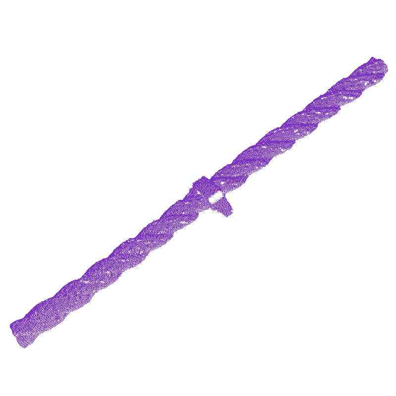
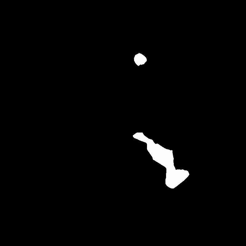
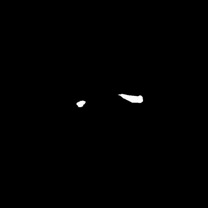
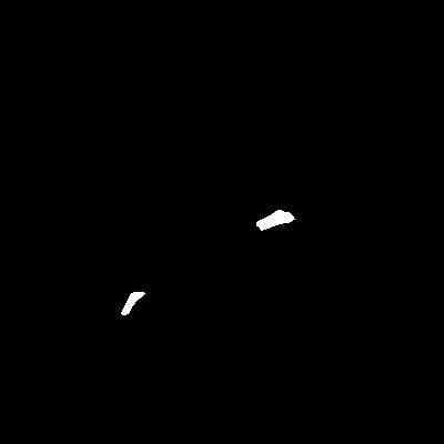
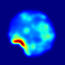
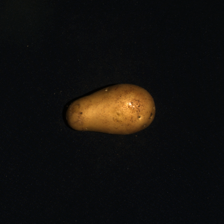
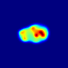
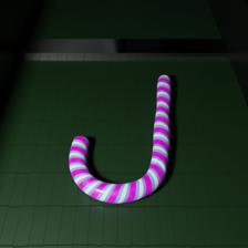
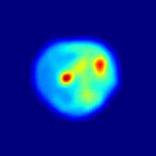
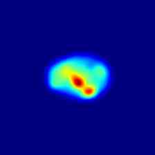
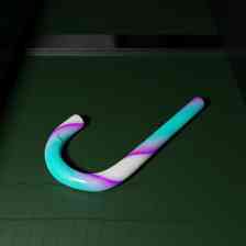
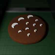
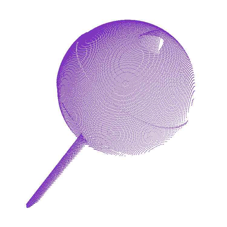
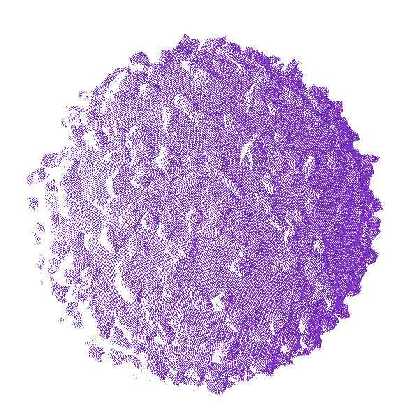
In Fig. 4, we highlight some failure cases of this approach. For instance, in the first left row, we note that our method cannot detect the missing left part of the cookie. Nevertheless, we predict higher anomaly scores for the area adjacent to the defect. In the second left row, the potato presents a tiny defect on its body, while the anomaly map — although covering the defect correctly — predicts a much broader anomaly. In the first and second right rows, the candy cane and the hazelnut truffle present high-frequency 2D or 3D patterns that produce higher anomaly scores compared to the real defects.

Finally, in Fig. 5 and Fig. 6 we show some additional qualitative results for all the classes of the MVTec 3D-AD and Eyecandies datasets, respectively. It is possible to notice how M3DM [42] tends to present anomalies on a broader area, highlighting the outline of the underlying object, while our method presents a more localized and less disturbed anomaly map.

RGB PC GT $\mathrm{\Psi }$ MVTec 3D-AD

RGB PC GT $\mathrm{\Psi }$ Eyecandies

Figure 4: Failure cases. Results on MVTec 3D-AD (left) and Eyecandies (right).

	Bagel	Cable Gl.	Carrot	Cookie	Dowel	Foam	Peach	Potato	Rope	Tire
RGB
PC
GT
M3DM
Ours
	Bagel	Cable Gl.	Carrot	Cookie	Dowel	Foam	Peach	Potato	Rope	Tire
RGB
PC
GT
M3DM
Ours

Figure 5: Qualitative results for each class of the MVTec 3D-AD dataset

	Can. C.	Cho. C.	Cho. P.	Conf.	Gum. B.	Haz. T.	Lic. S.	Lollip.	Marsh.	Pep. C.
RGB
PC
GT
M3DM
Ours
	Can. C.	Cho. C.	Cho. P.	Conf.	Gum. B.	Haz. T.	Lic. S.	Lollip.	Marsh.	Pep. C.
RGB
PC
GT
M3DM
Ours

Figure 6: Qualitative results for each class of the Eyecandies dataset

References

- Bergman et al. [2020] Liron Bergman, Niv Cohen, and Yedid Hoshen. Deep nearest neighbor anomaly detection. arXiv preprint arXiv:2002.10445, 2020.
- Bergmann et al. [2018] Paul Bergmann, Sindy Löwe, Michael Fauser, David Sattlegger, and Carsten Steger. Improving unsupervised defect segmentation by applying structural similarity to autoencoders. arXiv preprint arXiv:1807.02011, 2018.
- Bergmann et al. [2019] Paul Bergmann, Michael Fauser, David Sattlegger, and Carsten Steger. Mvtec ad – a comprehensive real-world dataset for unsupervised anomaly detection. In Proceedings of the IEEE/CVF Conference on Computer Vision and Pattern Recognition (CVPR), 2019.
- Bergmann et al. [2020] Paul Bergmann, Michael Fauser, David Sattlegger, and Carsten Steger. Uninformed students: Student-teacher anomaly detection with discriminative latent embeddings. In Proceedings of the IEEE/CVF conference on computer vision and pattern recognition, pages 4183–4192, 2020.
- Bergmann et al. [2022] Paul Bergmann, Jin Xin, David Sattlegger, and Carsten Steger. The mvtec 3d-ad dataset for unsupervised 3d anomaly detection and localization. In Proceedings of the 17th International Joint Conference on Computer Vision, Imaging and Computer Graphics Theory and Applications, pages 202–213, 2022.
- Bonfiglioli et al. [2022] Luca Bonfiglioli, Marco Toschi, Davide Silvestri, Nicola Fioraio, and Daniele De Gregorio. The eyecandies dataset for unsupervised multimodal anomaly detection and localization. In Proceedings of the 16th Asian Conference on Computer Vision (ACCV2022, 2022. ACCV.
- Cao et al. [2022] Yunkang Cao, Qian Wan, Weiming Shen, and Liang Gao. Informative knowledge distillation for image anomaly segmentation. Knowledge-Based Systems, 248:108846, 2022.
- Caron et al. [2021] Mathilde Caron, Hugo Touvron, Ishan Misra, Hervé Jégou, Julien Mairal, Piotr Bojanowski, and Armand Joulin. Emerging properties in self-supervised vision transformers. In Proceedings of the International Conference on Computer Vision (ICCV), 2021.
- Chang et al. [2015] Angel X. Chang, Thomas Funkhouser, Leonidas Guibas, Pat Hanrahan, Qixing Huang, Zimo Li, Silvio Savarese, Manolis Savva, Shuran Song, Hao Su, Jianxiong Xiao, Li Yi, and Fisher Yu. ShapeNet: An Information-Rich 3D Model Repository. Technical Report arXiv:1512.03012 [cs.GR], Stanford University — Princeton University — Toyota Technological Institute at Chicago, 2015.
- Chiu and Lai [2023] Li-Ling Chiu and Shang-Hong Lai. Self-supervised normalizing flows for image anomaly detection and localization. In Proceedings of the IEEE/CVF Conference on Computer Vision and Pattern Recognition, pages 2926–2935, 2023.
- Cohen and Hoshen [2020] Niv Cohen and Yedid Hoshen. Sub-image anomaly detection with deep pyramid correspondences. ArXiv, 2020.
- Defard et al. [2021] Thomas Defard, Aleksandr Setkov, Angelique Loesch, and Romaric Audigier. Padim: a patch distribution modeling framework for anomaly detection and localization. In International Conference on Pattern Recognition, pages 475–489. Springer, 2021.
- Deng and Li [2022] Hanqiu Deng and Xingyu Li. Anomaly detection via reverse distillation from one-class embedding. In Proceedings of the IEEE/CVF Conference on Computer Vision and Pattern Recognition, pages 9737–9746, 2022.
- Deng et al. [2009] Jia Deng, Wei Dong, Richard Socher, Li-Jia Li, Kai Li, and Li Fei-Fei. Imagenet: A large-scale hierarchical image database. In 2009 IEEE conference on computer vision and pattern recognition, pages 248–255. Ieee, 2009.
- Gudovskiy et al. [2022] Denis Gudovskiy, Shun Ishizaka, and Kazuki Kozuka. Cflow-ad: Real-time unsupervised anomaly detection with localization via conditional normalizing flows. In Proceedings of the IEEE/CVF Winter Conference on Applications of Computer Vision, pages 98–107, 2022.
- He et al. [2022] Kaiming He, Xinlei Chen, Saining Xie, Yanghao Li, Piotr Dollár, and Ross Girshick. Masked autoencoders are scalable vision learners. In Proceedings of the IEEE/CVF conference on computer vision and pattern recognition, pages 16000–16009, 2022.
- Horwitz and Hoshen [2023] Eliahu Horwitz and Yedid Hoshen. Back to the feature: classical 3d features are (almost) all you need for 3d anomaly detection. In Proceedings of the IEEE/CVF Conference on Computer Vision and Pattern Recognition, pages 2967–2976, 2023.
- Hou et al. [2021] Jinlei Hou, Yingying Zhang, Qiaoyong Zhong, Di Xie, Shiliang Pu, and Hong Zhou. Divide-and-assemble: Learning block-wise memory for unsupervised anomaly detection. In Proceedings of the IEEE/CVF International Conference on Computer Vision, pages 8791–8800, 2021.
- Kingma and Ba [2015] Diederik P. Kingma and Jimmy Ba. Adam: A method for stochastic optimization. In The International Conference on Learning Representations (ICLR), 2015.
- Kirillov et al. [2023] Alexander Kirillov, Eric Mintun, Nikhila Ravi, Hanzi Mao, Chloe Rolland, Laura Gustafson, Tete Xiao, Spencer Whitehead, Alexander C. Berg, Wan-Yen Lo, Piotr Dollar, and Ross Girshick. Segment anything. In Proceedings of the IEEE/CVF International Conference on Computer Vision (ICCV), pages 4015–4026, 2023.
- Kolesnikov et al. [2021] Alexander Kolesnikov, Alexey Dosovitskiy, Dirk Weissenborn, Georg Heigold, Jakob Uszkoreit, Lucas Beyer, Matthias Minderer, Mostafa Dehghani, Neil Houlsby, Sylvain Gelly, Thomas Unterthiner, and Xiaohua Zhai. An image is worth 16x16 words: Transformers for image recognition at scale. In International Conference on Learning Representations, 2021.
- Li et al. [2021] Chun-Liang Li, Kihyuk Sohn, Jinsung Yoon, and Tomas Pfister. Cutpaste: Self-supervised learning for anomaly detection and localization. In Proceedings of the IEEE/CVF conference on computer vision and pattern recognition, pages 9664–9674, 2021.
- Liu et al. [2023] Jiaqi Liu, Guoyang Xie, Jingbao Wang, Shangnian Li, Chengjie Wang, Feng Zheng, and Yaochu Jin. Deep industrial image anomaly detection: A survey. arXiv preprint arXiv:2301.11514, 2, 2023.
- Massoli et al. [2021] Fabio Valerio Massoli, Fabrizio Falchi, Alperen Kantarci, Şeymanur Akti, Hazim Kemal Ekenel, and Giuseppe Amato. Mocca: Multilayer one-class classification for anomaly detection. IEEE Transactions on Neural Networks and Learning Systems, 33(6):2313–2323, 2021.
- Oquab et al. [2023] Maxime Oquab, Timothée Darcet, Theo Moutakanni, Huy V. Vo, Marc Szafraniec, Vasil Khalidov, Pierre Fernandez, Daniel Haziza, Francisco Massa, Alaaeldin El-Nouby, Russell Howes, Po-Yao Huang, Hu Xu, Vasu Sharma, Shang-Wen Li, Wojciech Galuba, Mike Rabbat, Mido Assran, Nicolas Ballas, Gabriel Synnaeve, Ishan Misra, Herve Jegou, Julien Mairal, Patrick Labatut, Armand Joulin, and Piotr Bojanowski. Dinov2: Learning robust visual features without supervision, 2023.
- Pang et al. [2022] Yatian Pang, Wenxiao Wang, Francis EH Tay, Wei Liu, Yonghong Tian, and Li Yuan. Masked autoencoders for point cloud self-supervised learning. In Computer Vision–ECCV 2022: 17th European Conference, Tel Aviv, Israel, October 23–27, 2022, Proceedings, Part II, pages 604–621. Springer, 2022.
- Papamakarios et al. [2021] George Papamakarios, Eric Nalisnick, Danilo Jimenez Rezende, Shakir Mohamed, and Balaji Lakshminarayanan. Normalizing flows for probabilistic modeling and inference. The Journal of Machine Learning Research, 22(1):2617–2680, 2021.
- Pirnay and Chai [2022] Jonathan Pirnay and Keng Chai. Inpainting transformer for anomaly detection. In International Conference on Image Analysis and Processing, pages 394–406. Springer, 2022.
- Qi et al. [2017] Charles Ruizhongtai Qi, Li Yi, Hao Su, and Leonidas J Guibas. Pointnet++: Deep hierarchical feature learning on point sets in a metric space. In Advances in Neural Information Processing Systems. Curran Associates, Inc., 2017.
- Radford et al. [2021] Alec Radford, Jong Wook Kim, Chris Hallacy, Aditya Ramesh, Gabriel Goh, Sandhini Agarwal, Girish Sastry, Amanda Askell, Pamela Mishkin, Jack Clark, et al. Learning transferable visual models from natural language supervision. In International conference on machine learning, pages 8748–8763. PMLR, 2021.
- Reiss et al. [2021] Tal Reiss, Niv Cohen, Liron Bergman, and Yedid Hoshen. Panda: Adapting pretrained features for anomaly detection and segmentation. In Proceedings of the IEEE/CVF Conference on Computer Vision and Pattern Recognition, pages 2806–2814, 2021.
- Rippel et al. [2021] Oliver Rippel, Patrick Mertens, and Dorit Merhof. Modeling the distribution of normal data in pre-trained deep features for anomaly detection. In 2020 25th International Conference on Pattern Recognition (ICPR), pages 6726–6733. IEEE, 2021.
- Ristea et al. [2022] Nicolae-Cătălin Ristea, Neelu Madan, Radu Tudor Ionescu, Kamal Nasrollahi, Fahad Shahbaz Khan, Thomas B Moeslund, and Mubarak Shah. Self-supervised predictive convolutional attentive block for anomaly detection. In Proceedings of the IEEE/CVF conference on computer vision and pattern recognition, pages 13576–13586, 2022.
- Roth et al. [2022] Karsten Roth, Latha Pemula, Joaquin Zepeda, Bernhard Schölkopf, Thomas Brox, and Peter Gehler. Towards total recall in industrial anomaly detection. In Proceedings of 2022 IEEE Conference on Computer Vision and Pattern Recognition, pages 14298–14308, 2022.
- Rudolph et al. [2021] Marco Rudolph, Bastian Wandt, and Bodo Rosenhahn. Same same but differnet: Semi-supervised defect detection with normalizing flows. In Proceedings of the IEEE/CVF winter conference on applications of computer vision, pages 1907–1916, 2021.
- Rudolph et al. [2023] Marco Rudolph, Tom Wehrbein, Bodo Rosenhahn, and Bastian Wandt. Asymmetric student-teacher networks for industrial anomaly detection. In Winter Conference on Applications of Computer Vision (WACV), 2023.
- Rusu et al. [2009] Radu Bogdan Rusu, Nico Blodow, and Michael Beetz. Fast point feature histograms (fpfh) for 3d registration. In 2009 IEEE International Conference on Robotics and Automation, pages 3212–3217, 2009.
- Salehi et al. [2021] Mohammadreza Salehi, Niousha Sadjadi, Soroosh Baselizadeh, Mohammad H Rohban, and Hamid R Rabiee. Multiresolution knowledge distillation for anomaly detection. In Proceedings of the IEEE/CVF conference on computer vision and pattern recognition, pages 14902–14912, 2021.
- Sitzmann et al. [2020] Vincent Sitzmann, Julien N.P. Martel, Alexander W. Bergman, David B. Lindell, and Gordon Wetzstein. Implicit neural representations with periodic activation functions. In Proc. NeurIPS, 2020.
- Sohn et al. [2021] Kihyuk Sohn, Chun-Liang Li, Jinsung Yoon, Minho Jin, and Tomas Pfister. Learning and evaluating representations for deep one-class classification. In International Conference on Learning Representations, 2021.
- Wang et al. [2021] Guodong Wang, Shumin Han, Errui Ding, and Di Huang. Student-teacher feature pyramid matching for anomaly detection. In The British Machine Vision Conference (BMVC), 2021.
- Wang et al. [2023] Yue Wang, Jinlong Peng, Jiangning Zhang, Ran Yi, Yabiao Wang, and Chengjie Wang. Multimodal industrial anomaly detection via hybrid fusion. In Proceedings of the IEEE/CVF Conference on Computer Vision and Pattern Recognition, pages 8032–8041, 2023.
- Wyatt et al. [2022] Julian Wyatt, Adam Leach, Sebastian M Schmon, and Chris G Willcocks. Anoddpm: Anomaly detection with denoising diffusion probabilistic models using simplex noise. In Proceedings of the IEEE/CVF Conference on Computer Vision and Pattern Recognition, pages 650–656, 2022.
- Yang et al. [2020] Jie Yang, Yong Shi, and Zhiquan Qi. Dfr: Deep feature reconstruction for unsupervised anomaly segmentation. arXiv preprint arXiv:2012.07122, 2020.
- Yang et al. [2023] Minghui Yang, Peng Wu, and Hui Feng. Memseg: A semi-supervised method for image surface defect detection using differences and commonalities. Engineering Applications of Artificial Intelligence, 119:105835, 2023.
- Yi and Yoon [2020] Jihun Yi and Sungroh Yoon. Patch svdd: Patch-level svdd for anomaly detection and segmentation. In Proceedings of the Asian conference on computer vision, 2020.
- Yoa et al. [2021] Seungdong Yoa, Seungjun Lee, Chiyoon Kim, and Hyunwoo J Kim. Self-supervised learning for anomaly detection with dynamic local augmentation. IEEE Access, 9:147201–147211, 2021.
- Yu et al. [2021] Jiawei Yu, Ye Zheng, Xiang Wang, Wei Li, Yushuang Wu, Rui Zhao, and Liwei Wu. Fastflow: Unsupervised anomaly detection and localization via 2d normalizing flows. arXiv preprint arXiv:2111.07677, 2021.
- Zavrtanik et al. [2021] Vitjan Zavrtanik, Matej Kristan, and Danijel Skočaj. Draem-a discriminatively trained reconstruction embedding for surface anomaly detection. In Proceedings of the IEEE/CVF International Conference on Computer Vision, pages 8330–8339, 2021.
- Zhang and Deng [2021] Zheng Zhang and Xiaogang Deng. Anomaly detection using improved deep svdd model with data structure preservation. Pattern Recognition Letters, 148:1–6, 2021.