FOSS: A Self-Learned Doctor for Query Optimizer

Abstract

Various works have utilized deep reinforcement learning (DRL) to address the query optimization problem in database system. They either learn to construct plans from scratch in a bottom-up manner or guide the plan generation behavior of traditional optimizer using hints. While these methods have achieved some success, they face challenges in either low training efficiency or limited plan search space. To address these challenges, we introduce FOSS, a novel DRL-based framework for query optimization. FOSS initiates optimization from the original plan generated by a traditional optimizer and incrementally refines suboptimal nodes of the plan through a sequence of actions. Additionally, we devise an asymmetric advantage model to evaluate the advantage between two plans. We integrate it with a traditional optimizer to form a simulated environment. Leveraging this simulated environment, FOSS can bootstrap itself to rapidly generate a large amount of high-quality simulated experiences. FOSS then learns and improves its optimization capability from these simulated experiences. We evaluate the performance of FOSS on Join Order Benchmark, TPC-DS, and Stack Overflow. The experimental results demonstrate that FOSS outperforms the state-of-the-art methods in terms of latency performance and optimization time. Compared to PostgreSQL, FOSS achieves savings ranging from 15% to 83% in total latency across different benchmarks.

I Introduction

Query optimizer plays a critical role in database management system (DBMS). It takes a relational algebra expression derived from the parser as input and outputs an optimized physical execution plan. Most query optimizers follow the Selinger’s design and consist of the cardinality estimator, the cost estimator, and the query plan generator [1]. These components work together to explore the plan space and find the potentially optimal query plan.

However, for traditional query optimizer, finding the optimal plan within the vast plan space is an NP-hard problem [2]. Even if only the left-deep tree is considered in join order, the plan space still grows exponentially to $O(n!)$, where $n$ represents the number of tables involved in the query. The plan search space is further expanded when considering other factors, such as bushy tree, join methods and access path. Meanwhile, errors in traditional cardinality and cost estimator often result in poor-performance plans [2]. Furthermore, traditional query optimizer can not learn from the past experiences, often generating the similar poor-performance plans for the same queries repeatedly [3].

I-A Machine Learning for Query Optimization

To address the problem of traditional query optimizer, numerous studies focus on employing machine learning in end-to-end query optimization. We roughly categorize current methods into two types: plan-constructor and plan-steerer.
Plan-constructor. It is an expertise-omission approach that discards or underuses expert knowledge of traditional optimizer and focuses on constructing plans from scratch [4, 5, 6, 7, 8, 9]. It models the process of query plan generation as a Markov Decision Process (MDP) and uses deep reinforcement learning (DRL) to solve it. Its framework involves several components. An agent (i.e., a learned model) starts with a set of individual tables involved in the query, and at each step, it joins tables, joins subplans or specifies an operator. Each step results in a new state, which consists of a partial plan and other tables that have not been joined yet. The process continues until all tables involved in the query are joined, resulting in a complete plan. In this process, the DBMS serves as the environment and provides reward feedback, which are typically correlated with the execution cost or true execution latency of the final plans. Although plan-constructor can gradually surpass the performance of traditional query optimizer after a certain training period, it has the following drawbacks:

• (C1) Learning from scratch. The agent need to exert considerable effort to learn how to produce a cost-effective plan from scratch. This usually requires a significant amount of trial-and-error learning, gradually enabling the agent to reach a proficiency level similar to that of a traditional query optimizer.

• (C2) Poor experience sampling. Training a proficient agent requires a substantial amount of high-quality experiences. Prior approaches [4, 5, 6, 7, 9, 8] commonly employ cost estimation or execution latency as rewards to shape the experiences. Nevertheless, errors in cost estimation arising from the traditional cost model frequently lead to suboptimal outcomes. While using execution latency is more likely to generate superior plans, the low efficiency of obtaining execution latency incurs significant overhead. This inefficiency leads to the insufficient exploration problem, thus requiring a large amount of time for model convergence.

• (C3) Sparse reward. The number of steps required for an agent to complete the construction of a plan depends on the number of tables involved in the query. In Join Order Benchmark (JOB) [2], the queries have between 3 and 16 joins, with an average of 8 joins per query. However, prior methods such as [8, 7, 6, 10] encounter challenges in providing specific evaluations for subplans before obtaining the complete plan. In their scenarios, rewards are often assigned a value of 0 for the intermediate state, leading to sparse rewards for the agent and limiting access to sufficient guidance [11].

Plan-steerer. It is a blackbox-expertise approach that leverages the embedded expert knowledge in traditional query optimizer [12, 13, 14]. Guided by various hints, it generates multiple plans through the traditional query optimizer. For instance, in Bao [12], coarse-grained hints like disabling nested loop join for the entire query are used to guide the traditional query optimizer. It then utilizes a learned value network to evaluate these candidate plans and predict the cost. Ultimately, it selects the plan with the potentially lowest cost for execution. However, it has the following problems:

• (S1) Requiring expertise for hint design. While plan-steerer leverages traditional query optimizer to generate better plans through hints guidance, the design of hints still requires expert knowledge, as seen in the case of the hint set grouping in Bao [12].

• (S2) Limited search space. While some hints can steer traditional optimizer to select better plans, the coarse-grained nature of hints may limit plan-steerer to settling for the suboptimal plans.

• (S3) Hard to balance. Adding more candidate hints increases the number of candidate plans, thereby raising the probability of generating a better plan. However, this expansion also leads to an increase in optimization time.

I-B A Novel Framework for Query Optimization

In this paper, to alleviate the aforementioned problems, we introduce a novel framework FOSS that modify original plan step by step. FOSS can be categorized as plan-doctor, which is a whitebox-expertise approach. Unlike the blackbox-expertise approach that steers or constrains the traditional optimizer behavior, FOSS leverages expert optimization knowledge more explicitly by optimizing the plans generated by traditional query optimizer.

The insight behind FOSS is that although traditional query optimizer often produces suboptimal plans due to errors in cardinality estimation and cost estimation, much better plans can be retrieved by making a limited number of modifications to these suboptimal plans. For example, Query 1b from JOB takes $100.67ms$ to execute with plan generated by PostgreSQL’s optimizer. Due to the inaccurate cost estimation, the optimizer chooses a hash join operator between table $it$ and table $mi\mathrm{\_}idx$, which slows down the execution of plan. In this example, FOSS will first override the join method between the two tables to use a nested loop join, then exchange the positions of $it$ and $mi\mathrm{\_}idx$ to a proper order. With FOSS, the total execution latency reduces to $0.27ms$. In similar situations, FOSS acts like a doctor, identifying the suboptimal aspects causing performance issues in the given plan. It then takes actions, such as changing the physical implementation of the join node or rendering a proper order for two tables, in a step-by-step manner to optimize it.

However, to obtain an excellent plan-doctor, two key capabilities are essential: i) the ability to identify suboptimal aspects in the original plan and generate appropriate candidate action sequences for optimization. Note that different action sequences applied to the original plan will result in distinct new plans. ii) the ability to select the sequence that yields the optimal result for the original plan from candidates. To achieve these objectives, for i), FOSS learns a planner that models the identification of suboptimal aspects and the generation of action sequences as a MDP and employs DRL to solve it, and for ii), FOSS learns an asymmetric advantage model (AAM) to serve as the optimal action sequence selector. AAM determines the optimal sequence by evaluating the advantage values between pairs of candidate plans generated through candidate action sequences. Furthermore, inspired by model-based reinforcement learning (MBRL), FOSS integrates the AAM with a traditional optimizer to form a simulated environment, where the AAM serves as a reward indicator, and the traditional optimizer acts as a state transitioner.

We summarize the features of FOSS as follows:

• High training efficiency. FOSS starts from the original plans and focuses on optimizing suboptimal aspects, eliminating the need to learn from scratch (addressing C1). At each step, FOSS can generate a new complete execution plan, allowing for a straightforward evaluation of reward based on the performance of the new plan. Furthermore, the experimental results in VI demonstrate that FOSS often requires only 1-3 steps to achieve a better-performance plan (addressing C3). With the simulated environment, FOSS can efficiently bootstrap itself, generating ample high-quality simulated experiences to enhance its optimization capability (addressing C2).

• Intelligent candidate plans generation. FOSS can autonomously generate candidate plans through learning a planner, unlike plan-steerer’s reliance on pre-injected expert knowledge for hint design (addressing S1 and S3).

• Sufficient plan search space. FOSS employs finer-grained optimization, in contrast to plan-steerer’s coarse hints. Under similar scenarios, FOSS shares the same plan search space as plan-constructor, indicating its potential to discover the globally optimal plan (addressing S2).

Neither plan-constructor nor plan-steerer alone can encompass all of the aforementioned features. Therefore, FOSS strikes a good balance between the two approaches.

Figure 1: The framework of FOSS.

I-C Contributions

We summarize our contributions as follows:

• We introduce a whitebox-expertise approach called plan-doctor, which consists of a planner and a selector. It produces better-performance plans by optimizing the original plan through a step-by-step process.

• We construct a simulated environment and use simulated experiences to accelerate the learning of FOSS.

• We design an asymmetric advantage model to serve as a reward indicator in the simulated environment and as a selector to choose the optimal plan.

• Experimental results show that FOSS outperforms the state-of-the-art (SOTA) methods in terms of latency performance and optimization time, while also reducing total latency by 15% to 83% compared to the PostgreSQL.

II SYSTEM OVERVIEW

Figure 2: The workflow of planner.

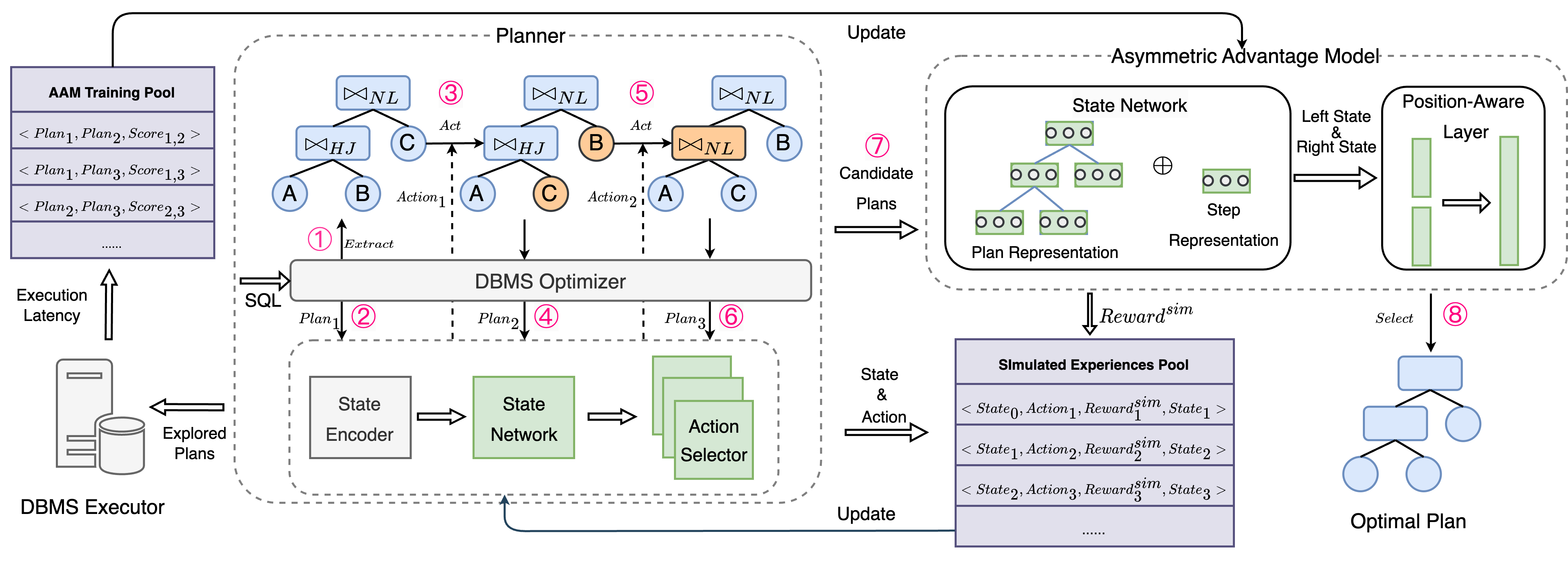
The overall architecture of FOSS is illustrated in Fig. 1. For a given query, FOSS follows the order indicated by the pink numbers to output the better-performance plan. Firstly, planner utilizes past experiences to iteratively modify the original plan, resulting in a set of potentially promising plans. Then, following the temporal sequence (i.e., the order of generated candidate plans), asymmetric advantage model (AAM) serves as the selector, assessing specific pairs of candidate plans and selecting the estimated optimal plan. To expedite the learning of the planner, FOSS builds a simulated learner to generate ample high-quality experiences. We divide our framework into the following three key modules.
Planner. We deploy the entire process of planner using DRL framework. Starting from the original plan, planner first encodes plan features. Considering the temporal nature of plans generated by planner, we incorporate the step status. These features are concatenated as the initial state and then passed to the agent. The agent first represents the state using a state network. Then the state representation is subsequently forwarded to the action selector to generate an action, which could involve operations such as swapping table positions or overriding join method. Following the execution of the action, a new plan is generated and forwarded to the reward function module to obtain rewards. Meanwhile, the new plan is utilized to generate a new state. This iterative process continues until the maximum step limit is attained. Experiences in the format $\{State,Action,Reward,Stat{e}_{{}^{\prime }}\}$ will be collected to update the agent. Through extensive training, planner can generate more optimal plans than the original plan.
Asymmetric Advantage Model. It serves as both optimal plan selector and the reward indicator in simulated environment. It consists of state network and position-aware output layer. First, we define the state network, which also helps the planner’s agent understand the state. Its primary architecture is based on the Transformer [15], which can efficiently capture the structural and node information of plans. It involves embedding plan features and step statuses separately, passing them through a multi-head attention network, ultimately outputting the state representations. For position-aware output layer, the input comprises the two state representations $stateve{c}_{left}$ and $stateve{c}_{right}$, while the output indicates the extent to which the $stateve{c}_{right}$ surpasses the $stateve{c}_{left}$. We map the output to different scores. The selection of the optimal plan and the evaluation of rewards is determined based on these scores.
Simulated Learner. In DBMS, the cost of using the traditional optimizer to generate plans is low. FOSS utilizes the traditional optimizer and AAM to form a simulated environment. Therefore, FOSS comprises three key components: the agent, the real environment, and the simulated environment. The agent of planner interacts with the real environment, which executes explored plans in the actual system to gather AAM training pool. These data are then used to update the AAM through a supervised learning process. Then, the agent will interact with the simulated environment to obtain simulated experiences, which will be used to update the agent. After several simulated learning iterations, we use the updated agent to continue interacting with the real environment, repeating the above process. Furthermore, we incorporate a dynamics timeout mechanism to ensure efficient data collection during the interaction with the real environment. We also integrate a validation mechanism. During simulated learning iterations, we select plans with high estimated performance, execute these plans to measure their execution latency, and then incorporate them into the AAM training pool.

III Planner

In this section, we will provide a detailed description of planner. Note that in current framework, we only consider left-deep plans, which is a structure frequently used in existing DBMS such as PostgreSQL and MySQL. Although we can explore bushy plans and incorporate modifications to the structure of plans in the action space, it significantly increases the size of the action space without necessarily yielding corresponding benefits. Therefore, for now, we focus solely on left-deep plans, leaving the consideration of bushy plans for future work.

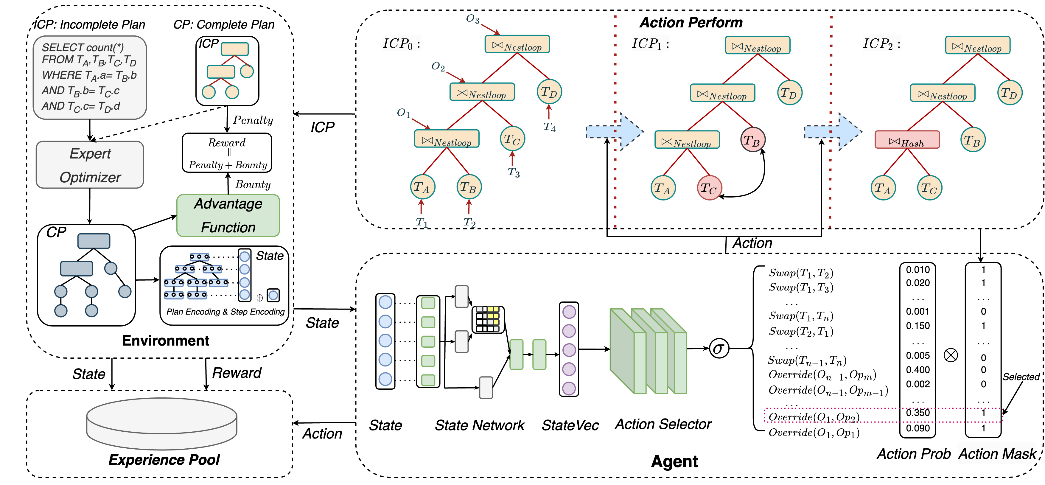
Given a schema with $n$ tables, when a query $Q$ is received, we obtain the complete plan $CP$ (i.e., execution plan) from the output of the traditional optimizer. We extract the key information from $CP$ that holds significant importance on the performance of plan. This yields an incomplete plan $ICP$, as shown in Fig. 2. The $ICP$ represents a subset of $CP$ and includes the join order and join method. The planner’s main process is to iteratively modify $ICP$ in a step-by-step manner. After taking one step on the $ICP$, guided by the new $ICP$, we can derive the new $CP$ using the DBMS hook, such as pg_hint_plan in PostgreSQL. When the maximum number of steps $maxsteps$ per episode is reached, the plan modification process will be stopped. Planner adopts the framework of DRL, which consists of key components like agent, environment, state, action and reward. Next, we will provide a detailed explanation of each component.
State. It is the output of the environment and the input to the agent. It is primarily composed of $CP$, typically in the form of tree-like structure. To facilitate the agent’s handling of $CP$, it is essential to extract critical information from the plan and encode it. We will provide the specific details of plan encoding in IV-A. Now, we use $PlanEncoding(CP)$ to represent the encoding of $CP$. Additionally, to incorporate the temporal characteristics of the state, we also include the $Step(t)=t/maxsteps$ in state. By concatenating these two types of features, we obtain the state features $State(C{P}_t)$ at time step $t$.

$$State(C{P}_t)=PlanEncoding(C{P}_t)||Step(t)$$ (1)

Action. First, we assign sequential labels to the nodes of the $ICP$ in a bottom-up fashion. We use two types of labels: $T_k$ to represent leaf nodes (i.e., tables) and $O_k$ to represent non-leaf nodes (i.e., join methods). As shown in Fig. 2, we start with the two leaf nodes at the deepest level, where the left node is labeled as $T_1$ and the right node as $T_2$. The leaf node at the level above them are labeled as $T_3$, and so on. Similarly, we label the deepest non-leaf node as $O_1$, its parent node as $O_2$, and so forth, following the bottom-up sequence.

Next, we will explain the representation of two types of action. The first type is swapping the positions of two tables $(T_l,T_r)$, represented as $Swap(T_l,T_r)$. There are $nu{m}_s=(n\times (n-1))/2$ different actions for table positions swapping. The second type is overriding the join method of node $O_i$ with the $j$-th join method in $Op$, represented as $Override(O_i,O{p}_j)$, where $Op$ is the set of all available join methods in DBMS. There are $nu{m}_o=\left|Op\right|\times (n-1)$ different actions for overriding join method. Action is encoded as an integer $a$ within the range $[1,nu{m}_s+nu{m}_o]$. We define an action mapping function $Act(a,ICP)$ which maps an integer $a$ to the corresponding action behavior on $ICP$. We can represent it as follows:

(2)

, where the integer in $Rang{e}_s=[1,nu{m}_s]$ represents table positions swapping action, and the integer in $Rang{e}_o=[nu{m}_s+1,nu{m}_s+nu{m}_o]$ represents join method overriding action. If $a$ satisfies $Rang{e}_s$, the $Swap(T_l,T_r)$ is called, where $l$ and $r$ satisfy the following conditions:

. If $a$ satisfies $Rang{e}_o$, the $Override(O_i,O{p}_j)$ is called, where $i$ and $j$ satisfy the following conditions:

$$\{\begin{array}{cc}i=\lceil \frac{nu{m}_s+nu{m}_o+1-a}{\left|Op\right|}\rceil \hfill & \\ j=(nu{m}_s+nu{m}_o-amod\left|Op\right|)+1\hfill & \end{array}$$

. However, each query may have different action space restrictions, depending on the number of tables in the query graph. For example, in the query shown in Fig. 2, $Swap(T_1,T_5)$ is considered an illegal action. To address the problem, we perform a validity check on the action space before the agent selects an action. We use $actionmask$ to prohibit illegal actions. To further prune the action space, we employ a heuristic rule. After execute $Swap(T_l,T_r)$, the subsequent action can only select how to override the join method related to the two tables that were swapped in the previous step. This also be implemented using the $actionmask$.
Reward. During the training process of planner, we maintain both the known best plan $C{P}_b^q$ for each query and the best plan $C{P}_b^p$ perceived by FOSS. And at each step $t$ of one episode $e$, a new incomplete plan $IC{P}_t^e$ and a new complete plan $C{P}_t^e$ will be generated. We determine reward based on these plans. The reward at each step $Rewar{d}_t^e$ is the sum of bounty $Bount{y}_t^e$ and penalty $Penalt{y}_t^e$. And the reward for each episode is the sum of reward obtained at each step.
Bounty. First, we define the initial advantage function $Ad{v}_{initial}$ to calculate the initial advantage value between two plans, indicating how much better $C{P}_r$ is compared to $C{P}_l$.

$$Ad{v}_{initial}(C{P}_l,C{P}_r)=\frac{U(C{P}_l)-U(C{P}_r)}{U(C{P}_l)}$$

, where $U(CP)$ is related to the performance of $CP$. However, fine-grained value is unsuitable for dynamically changing system workloads. We discretize initial advantage value into several intervals. We take an $l$-element finite ordered point set and use it to partition the interval $(-\mathrm{\infty },1]$ into $l+1$ subintervals, resulting in the set of ordered subintervals $D=\{(d_i,d_{i+1}]|i\in \{0,1,\mathrm{\dots },l\},d_0\to -\mathrm{\infty },d_{l+1}=1\}\}$. We use $D_k$ to represent the $k$-th element (i.e., subinterval) in $D$ and set ${\widehat{D}}_k=(d_k+d_{k-1})/2$. We define the final advantage function $Adv$ that takes a pair of plans as input and outputs a score.

$$Adv(C{P}_l,C{P}_r)=k-1\text{if}Ad{v}_{initial}(C{P}_l,C{P}_r)\in D_k$$ (3)

In each episode, we maintain the current best plan $C{P}_b^e$. At each step, we calculate $Adv(C{P}_b^e,$ $C{P}_t^e)$ and provide a step bounty $c{b}_t^e$:

$$c{b}_t^e=Adv(C{P}_b^e,C{P}_t^e)\times \eta ,\eta >0$$

. Additionally, if current step is $maxsteps$, we will append the episode bounty $e{b}^e$. We begin by defining $e{b}^{pb}$ and $e{b}^{qb}$ to represent the FOSS’s episode bounty and known best episode bounty.

$$e{b}^{pb}=Ad{v}_{initial}(C{P}_o^q,C{P}_b^p)\times e{b}^m$$

$$e{b}^{qb}=Ad{v}_{initial}(C{P}_o^q,C{P}_b^q)\times e{b}^m$$

, where $e{b}^m$ represents the maximum episode bounty. Then we calculate the advantage values $ad{v}_1=Adv(C{P}_b^q,C{P}_b^e)$, $ad{v}_2=Adv(C{P}_b^p,C{P}_b^e)$, and $ad{v}_3=Adv(C{P}_o^q,C{P}_b^e)$. The episode bounty $e{b}^e$ can be represented as follows:

. Finally, we obtain the $Bount{y}_t^e$ as follows:

$$Bount{y}_t^e=c{b}_t^e+\lfloor \frac{t}{maxsteps}\rfloor \times e{b}^e.$$

Penalty. To encourage the agent to reach each different state with as few steps as possible, we implement a penalty measure. In planner, reaching a certain state from the initial state can involve multiple action sequences of varying lengths, where an action sequence refers to a combination of $Swap$ and $Override$ operators. In order to gain more rewards, the agent may opt for inappropriate action sequences. For example, assume that the execution latency for the hash join operator at position $O_i$ is $L_1$, $L_2$ for merge join, and $L_3$ for nested loop join. Suppose $L_1>L_2>L_3$, and the original plan choose using hash join. In order to obtain more bounty, the agent may choose to initially override the method at $O_i$ to a merge join, and then in subsequent steps, override it to a nested loop join. To address such issue, we calculate the minimum number of steps required from the original incomplete plan to the current incomplete plan, denoted as $minsteps(IC{P}_t^e)$. Additionally, we introduce a penalty coefficient $\gamma >0$. We set the penalty value according to the following formula:

$$Penalt{y}_t^e=\gamma \times (minsteps(IC{P}_t^e)-t)$$ (4)

. If the current step is already the minimum, the penalty value will be 0. Otherwise, it will have a negative impact on the reward. It ensures that the agent can learn useful knowledge more effectively.

In FOSS, $\eta$ is set to 0.5, $e{b}^m$ is set to 12 and $\gamma$ is set to 2.
Agent. In planner, the agent mainly consists of two models: the state network $\varphi$ and the action selector $\pi$. The former is a transformer-based network used to process the state. It takes the state $s$ as input and outputs the state representation vector $statevec$. Further details about the state network will be explained in IV-A. We use multi-layer fully connected neural network to serve as the action selector. It takes the $statevec$ and the $actionmask$ as input and outputs the action encoding $a$ that maximizes the cumulative expected reward.

$$\varphi (s)\to statevec,\pi (statevec,actionmask)\to a$$

Environment. Its main functions include: i) providing new state based on the action taken by the agent; ii) assessing the agent’s action to provide reward. For i), we use the DBMS optimizer ${\mathrm{\Gamma }}_p$ to provide new state. We can express it using the following formula:

. In the case of the initial step, it takes the query $Q$ as input and outputs a complete plan $CP$. In non-initial steps, it takes both the incomplete plan $ICP$ and the query $Q$ as input, generating a complete plan $CP$ steered by $ICP$. We can then encode the $CP$ to obtain the new state by using (1). For ii), after obtaining $CP$, we provide a reward as described in the part of Reward. The key difference is that in the real environment, we use the DBMS executor ${\mathrm{\Psi }}_p$ to execute the plan and then use the execution latency to represent the performance of plan $U(CP)$. Subsequently, we calculate the advantage and the final reward. In the simulated environment, the advantage value is evaluated by asymmetric advantage model without executing the plan. The specific details will be discussed in IV-B.

Algorithm 1 Planner Training Process

1:for Query $Q$ in Workload $W$ do

2: $C{P}_0\leftarrow {\mathrm{\Gamma }}_p(Q,/)$

3: $IC{P}_0\leftarrow Extract(C{P}_0)$

4: HistoryPlanSet $T=[IC{P}_0]$

5: EstimatedBestPlan $C{P}_{best}=C{P}_0$

6: for $t=1\to maxsteps$ do

7: $actionmask\leftarrow IC{P}_{t-1}$

8: if $t>1\cap a_{t-1}\in Rang{e}_s$ then

9: $actionmask\leftarrow LimitSpace(actionmask)$

10: end if

11: $s_{t-1}=State(C{P}_{t-1})$

12: $stateve{c}_{t-1}=\varphi (s_{t-1})$

13: $a_t=\pi (stateve{c}_{t-1},actionmask)$

14: $IC{P}_t=Act(a_t,IC{P}_{t-1})$

15: $C{P}_t\leftarrow {\mathrm{\Gamma }}_p(Q,IC{P}_t)$

16: $r_t=Penalt{y}_t$

17: if $IC{P}_t\notin T$ then

18: $r_t=r_t+Bount{y}_t$

19: $AddIC{P}_{t}toT$

20: end if

21: $C{P}_{best}\leftarrow C{P}_t\text{if}Adv(C{P}_{best},C{P}_t)>0$

22: $experiences\leftarrow Collect(s_{t-1},a_t,r_t,s_t)$

23: end for

24:end for

25:$UpdateAgent(experiences)$

Algorithm 1 shows the overall training process of planner. When a query $Q$ of a workload $W$ is inputted, the DBMS optimizer generates the original plan $C{P}_0$ (Line 2). From $C{P}_0$, the planner extracts an incomplete plan $IC{P}_0$ composed of the join order and join methods (Line 3). The planner initializes the history plan set $T$ and the estimated best plan $C{P}_{best}$ (Line 4-5). For every step, the planner calculates the forbidden actions based on the $IC{P}_{t-1}$ (Line 7). If the previous action is $Swap$ operator, the current action will be restricted to only changing the adjacent join method (Line 8-10). Next, the planner represents the previous state based on the $C{P}_{t-1}$ and step status (Line 11-12) and evaluates the action based on the state representation $stateve{c}_{t-1}$ and $actionmask$ (Line 13). Then it applies this action to $IC{P}_{t-1}$ and produces a new incomplete plan $IC{P}_t$ (Line 14). The $IC{P}_t$ will be completed by the DBMS, resulting in a complete plan $C{P}_t$ (Line 15). The planner computes the penalty value and uses it to initialize the reward value (Line 16). If the current incomplete plan $IC{P}_t$ has not appeared in this episode, we add the bounty to reward and add the $IC{P}_t$ to $T$ (Line 17-20). If the current plan is better than the optimal plan, the planner updates the estimated optimal plan $C{P}_{best}$ (Line 21). Experiences are collected in order to update the agent (Line 22). Finally, upon concluding the exploration of the current workload, the agent is updated using $experiences$ (Line 25).

IV Asymmetric Advantage Model

In this section, we will provide a detailed description of the asymmetric advantage model. We begin by introducing the state representation, followed by the advantage model. Finally, we will discuss the design of the loss function.

IV-A State Representation

As mentioned in (1), state consists of both plan encoding and step encoding. We have introduced step encoding. Next, we will provide a detailed explanation of how we encode the complete plan. Finally, we will introduce the state network which transforms state to state representation.
Plan Encoding. Our work is structured based on the QueryFormer [16], which is a tree transformer model for query plan representation. Following their work, we first extract node features, including operators, predicates, joins, and tables. But we abstain from employing histogram data and sampling information due to computational efficiency concerns. To capture the node structural features of the query plan, we encode the height of nodes, which is defined as the length of the longest downward path from the node to a leaf node in the plan tree. Additionally, different from [16], we encode the structure type of each node. We classify nodes into four types: left nodes, right nodes, no-siblings nodes, and root nodes. We use the labels 0, 1, 2, and 3 to represent these four types of nodes, obtaining the node structure feature. To capture the tree structural features of the plan, we utilize attention network with attention mask. As the original attention network will attend to all nodes in the plan tree, which is not entirely reasonable, we aim to focus the attention network on meaningful structural information. To achieve this, we mask the mutual influence between unreachable nodes in the query plan tree, setting the attention score to 0 between two unreachable nodes and 1 between two reachable nodes. It differs from their work, which uses biased weights to adjust attention scores among nodes at different levels. We argue that assuming the same level of difference affects attention scores similarly is not reasonable for different nodes in various query plans or within the same query plan. This limitation hinders the model’s power.
State Network. We individually pass the extracted four types of node features through specific embedding layers to obtain the vector representation of each feature. Subsequently, we concatenate the four vectors to obtain the node representation, denoted as $N_i$, for the $i$-th node. We use dedicated embedding layers to represent the height and node structure features, obtaining $heigh{t}_i$ and $n{s}_i$ for each node. Finally, we concatenate $N_i$, $heigh{t}_i$, $n{s}_i$ and feed them into the multi-head attention network with attention scores. This process ultimately yields the representation of the query plan. Subsequently, it is concatenated with the step encoding and passed through a linear layer to generate the final state representation vector $statevec$.

IV-B Advantage Model

As described in (3), we need to calculate the advantage between two plans. In the real environment, precise advantage values can be obtained by executing the plans using DBMS executor. In simulated environment, we estimate the advantage values using an advantage model which takes plan pairs $(C{P}_l,C{P}_r)$ as input. It initially encodes the two input plans separately, transforming them into $(stateve{c}_l,stateve{c}_r)$ using the state network. Next, it incorporates position information for each $statevec$ to obtain $(stateve{c}_l\oplus po{s}_{left},stateve{c}_r\oplus po{s}_{right})$. Finally, the pair is passed to the final output layer, where it’s mapped to the scores (i.e., the output of $Adv$). The asymmetric advantage model ${\theta }_{adv}$ can be described as follows:

, where $FC$ represents fully-connected network. In the simulated environment, ${\theta }_{adv}$ serves as the advantage function $Adv$, and training data in the format $\{(C{P}_l,C{P}_r),Adv(C{P}_l,C{P}_r)\}$ will be used to update ${\theta }_{adv}$.

Considering that the dynamic changes in system workload may cause the labels of plan pairs with similar execution latency to change continuously and to select significantly superior plans, we take the point set $\{0.05,0.75\}$ to divide the interval $(-\mathrm{\infty },1]$, resulting in three scores (i.e., $\{0,1,2\}$) for the output of the $Adv$.

IV-C Asymmetric Loss

Since plans obtained from traditional optimizer are often of reasonable performance, starting with such plans as baselines and making modifications often yields more inferior plans. As a result, training samples for ${\theta }_{adv}$ are skewed towards a larger number of samples with a score of 0 and fewer samples with a score of 2. This uneven distribution of samples across different labels will adversely affect the training of the ${\theta }_{adv}$. Inspired by Asymmetric Loss [17], FOSS addresses the issue by increasing the weights of difficult-to-classify samples. Additionally, to prevent overfitting during training, FOSS also employs label smoothing.

For a given training samples set $\{x_i=(C{P}_l^i,C{P}_r^i),y_i=Adv(C{P}_l^i,C{P}_r^i)|i=1,2,\mathrm{\dots },N\}$, where $N$ represents the number of training samples, we employ one-hot encoding $h_{i,j}$ to represent the true label $y_i$:

. We use $Softmax$ to convert the output of ${\theta }_{adv}$ into score probability distribution. $p_{i,j}$ represents the probability of the $j$th label in the $i$th sample, and ${\widehat{p}}_{i,j}$ indicates the sample’s classification difficulty. Smaller ${\widehat{p}}_{i,j}$ values suggest higher difficulty, and vice versa.

(5)

To make ${\theta }_{adv}$ pay more attention to difficult-to-classify samples, FOSS introduces a decay factor of ${(1-{\widehat{p}}_{i,j})}^{\gamma }$, where $\gamma$ represents the decay coefficient. To emphasize the contribution of positive samples, we assign different decay coefficient to positive and negative samples. We denote the decay coefficient for positive samples as ${\gamma }_{+}$ and the decay coefficient for negative samples as ${\gamma }_{-}$ and set . This is represented by the following formula:

. We modify the probability distribution as follows:

, where $ϵ$ is a hyperparameter and $K$ represents the number of scores. In FOSS, $K$ is set to 3 and $ϵ$ is set to 0.1. The final loss function can be expressed as follows:

$$LOSS=-\sum _{i=1}^N\sum _{j=1}^K{\widehat{h}}_{i,j}{L}_{i,j}.$$

V Simulated Learner

In this section, we will begin by introducing the simulated environment. Next, we will provide an explanation of how FOSS explores the real environment and trains the agent using the simulated environment.

V-A Simulated Environment

As described in Algorithm 1, data in the form of $\{s,a,r,s^{{}^{\prime }}\}$ are collected to update the agent. However, in many environments, obtaining the real state and reward is challenging due to high costs or security concerns. To overcome this challenge, researchers propose simulating environment using neural networks to accelerate agent’s learning. An simulated environment always includes State Transition Dynamics Model ${\theta }_p(s,a)\to s^{{}^{\prime }}$ and Reward Function Model ${\theta }_r(s,a)\to r$ [18]. They will have the agent interact with the real environment and then use the real experiences to perform supervised training of the simulated environment [19]. Then the agent efficiently interacts with the simulated environment to generate simulated experiences, which are then used to update the agent accordingly.

In the context of planner, state is consist of complete plan $CP$ and step status, while step status is determined and $CP$ can be obtained from DBMS optimizer with low cost, especially within the guidance of $ICP$. Therefore, we can assign ${\theta }_p(s,a)$ with DBMS optimizer ${\mathrm{\Gamma }}_p$. However, obtaining the true reward requires executing the complete plan, which can be time-consuming. We only need to be aware of how we can simulate ${\theta }_r(s,a)$ to provide rewards feedback timely. Using the asymmetric advantage model ${\theta }_{adv}$ that we have established to assign rewards is a natural idea. Therefore, we employ the DBMS optimizer ${\mathrm{\Gamma }}_p$ and ${\theta }_{adv}$ to construct a simulated environment $\widehat{E}({\mathrm{\Gamma }}_p,{\theta }_{adv})$.

V-B Training Loop

In this subsection, we will discuss how to train the agent of the planner effectively using the simulated environment and the real environment, and how to collect training data for updating ${\theta }_{adv}$. It can be divided into three stages: the exploration phase, the training phase and the validation phase.
Exploration Phase. For a batch of training workload queries, the agent interacts with real environment to perform plan exploration and collect the execution latency into execution buffer. However, during the initial stage of exploration, agent is possible to generate catastrophic plans that are significantly worse than the original plan, and it may even lead to timeouts, significantly slowing down the exploration phase. To address this issue, we introduce dynamic timeouts to terminate the execution of poorly performing plans. The timeout is set to $1.5$ times the original plan’s execution latency. If the execution latency of a new generated plan exceeds this threshold, it is terminated and labeled as timeout. Then, as described in IV-B, we utilize the data in execution buffer to form the training data for ${\theta }_{adv}$ and update it. We will filter out plan pairs that involve timeouts for both. Although the timeout strategy results in a loss of training samples, it significantly increases the data collection rate.
Training Phase. FOSS randomly samples from the history queries and acquires simulated experiences by interacting with the simulated environment $\widehat{E}({\mathrm{\Gamma }}_p,{\theta }_{adv})$, following the process outlined in the Algorithm 1. Meanwhile, FOSS will collect excellent plans based on the outcomes of ${\theta }_{adv}$.
Validation Phase. FOSS executes the plans collected during the training phase, records their execution latency into the execution buffer, and updates ${\theta }_{adv}$ accordingly. This process enables the timely rectification of errors in ${\theta }_{adv}$, preventing the accumulation of errors in DRL training due to inaccuracies in reward estimation.
Global Process. FOSS initiates an exploration phase, succeeded by multiple rounds of training phases and a validation phase after each training iteration. This cyclic process is repeated several times until the FOSS converges. The three stages can be conducted interactively or simultaneously.

VI Experiments

In this section, we outline our experimental configurations and analyze the performance of FOSS while also conducting comparisons with SOTA methods. Finally, we analyze the effects of various components of FOSS and demonstrate the additional features of FOSS.

VI-A Experiment Setup

Experiment Support. We deploy FOSS alongside the SOTA methods on an Ubuntu 20.04 system, featuring a hardware configuration that includes a 2.40GHz Intel Xeon E5-2640 CPU, 256GB of memory, and an NVIDIA Tesla P40 GPU. We implement FOSS using PyTorch and utilize Ray [20] for the RL component. We utilize PPO [21] as the base RL algorithm due to its effectiveness in mitigating significant differences in the action distribution before and after agent updates through KL divergence. It further ensures the accuracy of the estimated reward provided by ${\theta }_{adv}$ in the simulated environment.
Workloads. We evaluate the performance of all the optimizers on three different benchmarks: Join Order Benchmark (JOB) [2], TPC-DS[22], and Stack [12].
JOB builds on the real-world IMDb dataset, which consists of 21 relations with a total data size of 3.6GB. Within the JOB workload, there are 33 query templates, encompassing 113 individual queries. We follow Balsa’s [8] random partitioning, splitting queries into 94 for training and 19 for testing.
TPC-DS is a standard benchmark. We utilize its data generation tool to create a dataset of 10GB in size. It includes 99 query templates. Nevertheless, a majority of these templates do not meet the requirements of some SOTA methods (such as requiring select-project-join queries) and the left-deep constraint of FOSS. We eventually opt for 19 query templates. From each template, we generate 6 individual queries, and from these, we randomly select 5 queries for the training workload and the remaining 1 query for the testing workload.
Stack comprises 18 million questions and answers collected from StackExchange websites such as StackOverflow.com over a decade. It is generated by [12] and occupy a total space of 100GB. Within the workload, there are 16 query templates. Similar to TPC-DS, we filter out the templates that do not meet the requirements and then randomly select 10 queries from the remaining 12 templates. For each template, 8 queries are assigned for the training workload, and 2 queries for testing.
Comparision. We employ PostgreSQL as baseline and compare FOSS with the SOTA methods, including Bao [12], Balsa [8], and HybridQO [14].
PostgreSQL is an open-source DBMS with a traditional optimizer. We employ it as a representative of traditional optimizer.
Bao follows plan-steerer framework. It steers traditional optimizer to select better query plans by employing a value model to choose different arms (i.e., hint sets). By default configuration, it has 5 arms available. We configure it according to the instructions provided in their documents [23].
Balsa is an end-to-end query optimizer that operates independently from traditional optimizer, following plan-constructor framework. We follow the instructions outlined in its source code [24] to deploy it .
HybridQO combines learned-based optimizer with traditional optimizer. It also follows plan-steerer framework. It employs Monte Carlo Tree Search to discover promising leading join order and uses these as hints to guide traditional optimizer in generating better query plans. We replicate their experimental setup as described in [25].
Expert Engine. For a fair comparison, We conduct all experiments using PostgreSQL 12.1. We set up PostgreSQL with 32GB shared buffers and disable GEQO due to the usage of pg_hint_plan. We employ it as the expert engine in our experiments.
Metrics. We deploy all learned query optimizers on the training workload and evaluate their performance on the testing workload using the two metrics: i) Workload Relevant Latency (WRL): it primarily reflects the overall latency level of the entire workload, as previously employed in the approach [13, 8, 9]. Its computation involves the ratio of the total latency of the entire workload executed by the learned-based optimizer to the total latency observed in expert optimizer. ii) Geometric Mean Relevant Latency (GMRL): it is introduced in [6] and demonstrates the optimization effectiveness at the query level. It can be expressed using the formula $GMRL=\sqrt[|W|]{{\prod }_{q\in W}\frac{E{T}_{learned}(q)}{E{T}_{expert}(q)}}$, where $E{T}_{learned}$ and $E{T}_{expert}$ respectively represent the execution latency of the learned-based optimizer and the expert optimizer. For the two metrics, a smaller value indicates better performance. A value greater than 1 implies inferiority compared to the expert optimizer, while a value less than 1 signifies the opposite.

VI-B FOSS Performance and Comparison

Unless specified otherwise, we set the $maxsteps$ to 3, explore 10 queries in each round of the exploration phase, and use 900 episodes (i.e., 900 queries) for each update of agent during training phase. We deploy all methods on each benchmark, running them five times with different random seeds.

(a) Training workload

(b) Testing workload

Figure 3: The relative speedup of FOSS compared to other methods across various workloads.

VI-B1 FOSS Performance Overview

(a) WRL of JOB

(b) WRL of TPC-DS

(c) WRL of STACK

(d) GMRL of JOB

(e) GMRL of TPC-DS

(f) GMRL of STACK

Figure 4: The training curves of FOSS on various workloads.

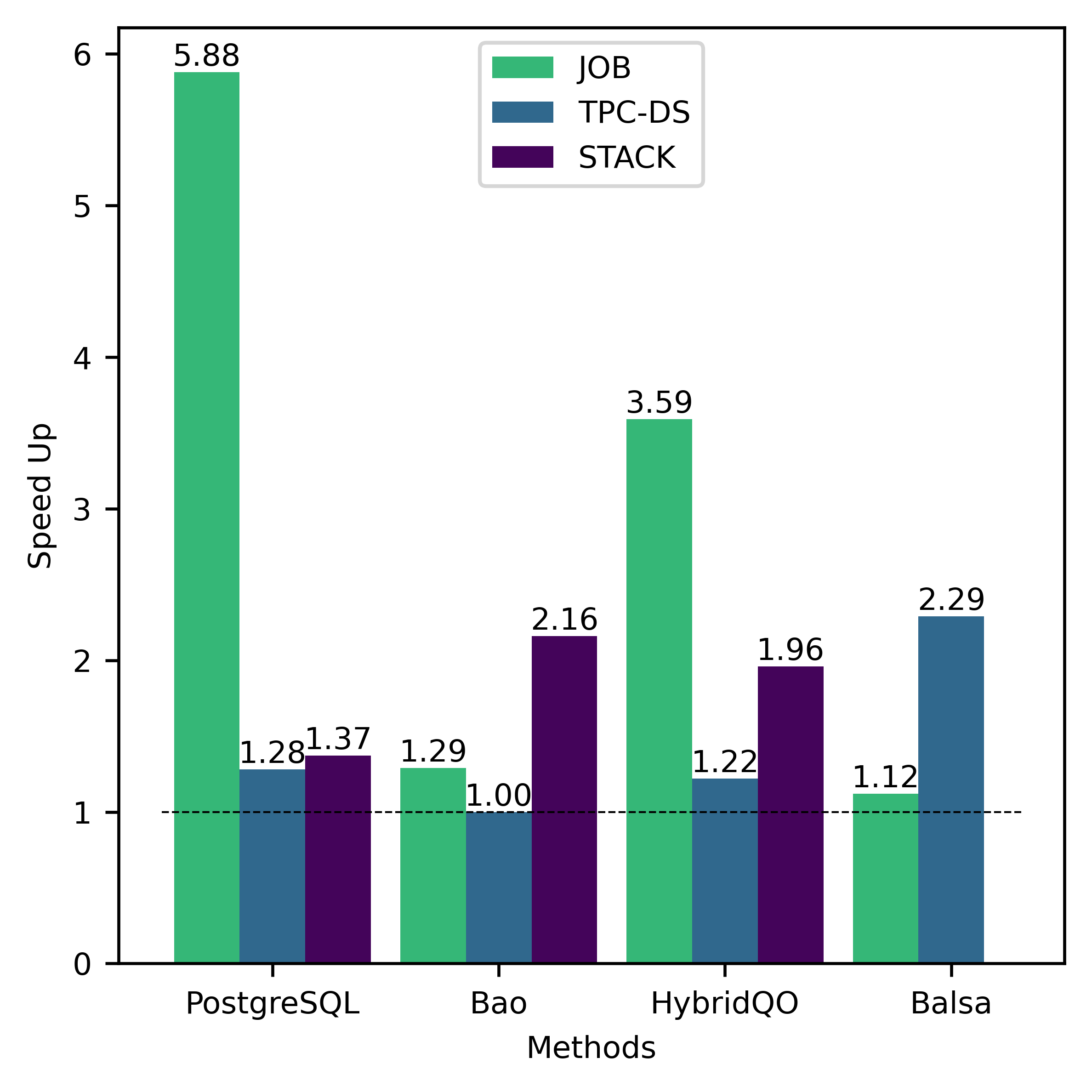
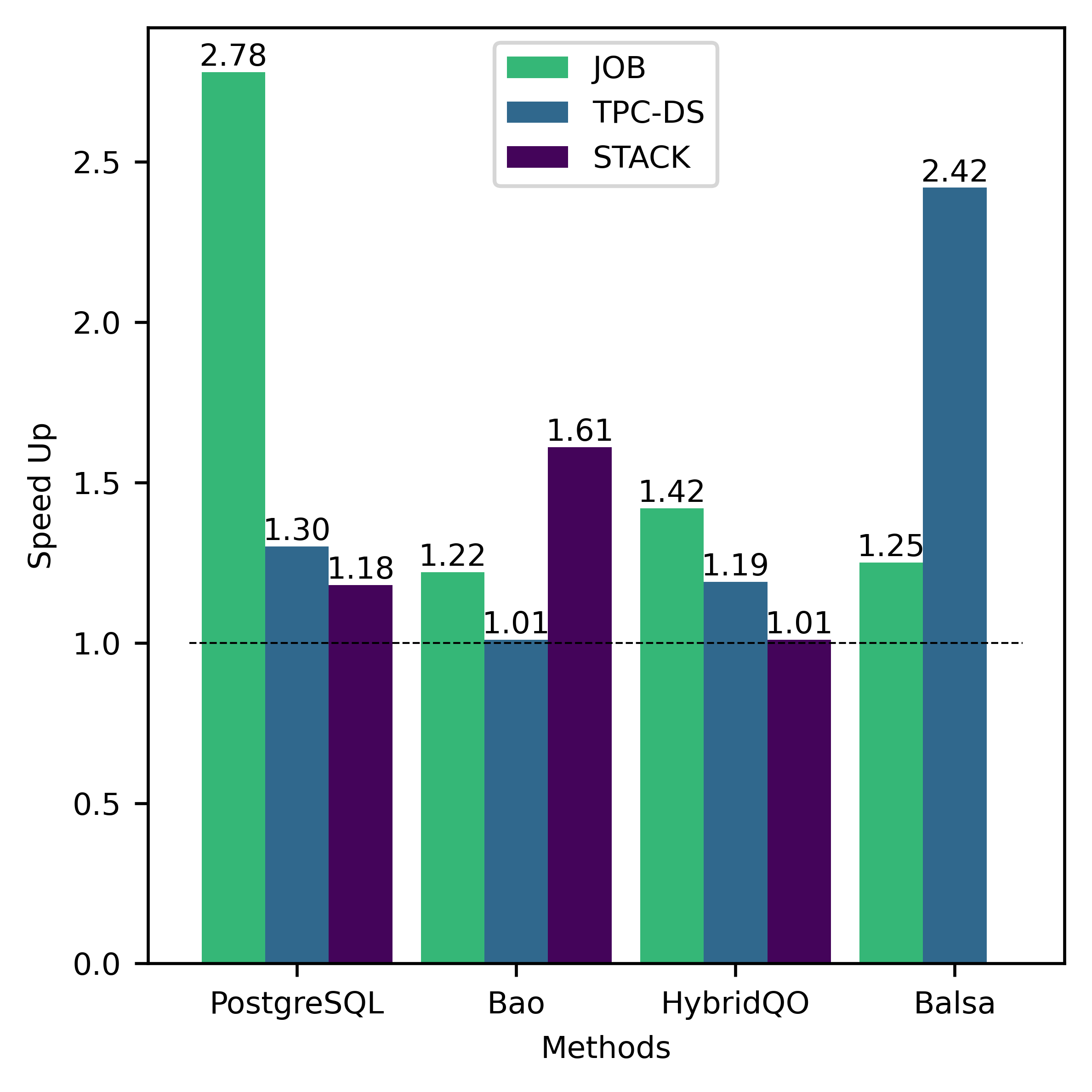
In this subsection, we analyze the training efficiency and performance of FOSS. Overall, FOSS outperforms the expert optimizer (i.e., PostgreSQL optimizer) with speedup of 5.88×, 1.28×, and 1.37× in total latency for the training workload (JOB, TPC-DS, STACK) and 2.78×, 1.30×, and 1.18× for the testing workload, respectively (Fig. 3).

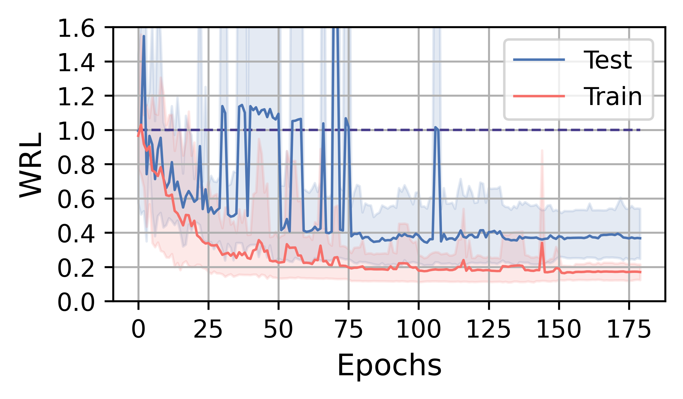
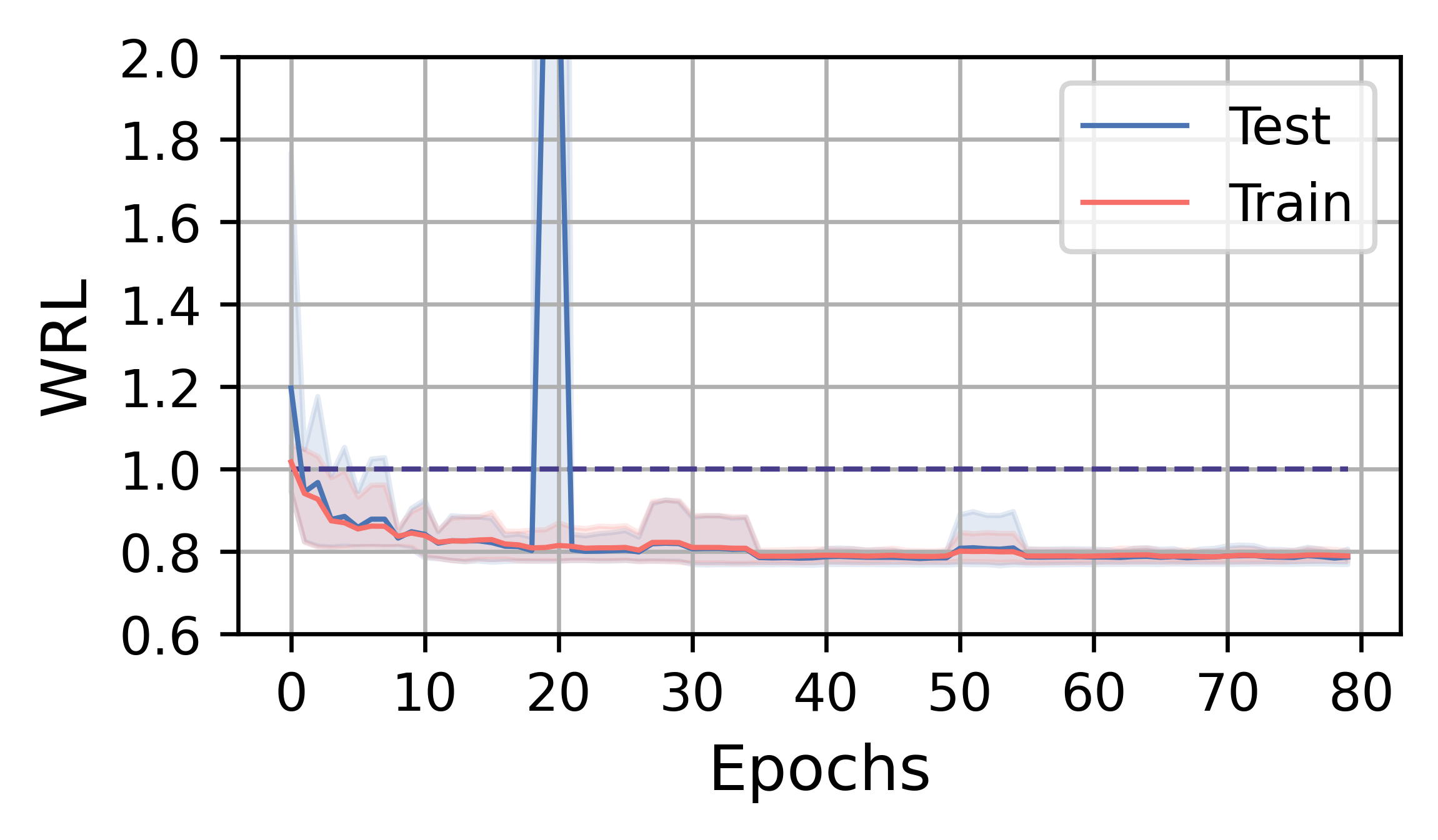
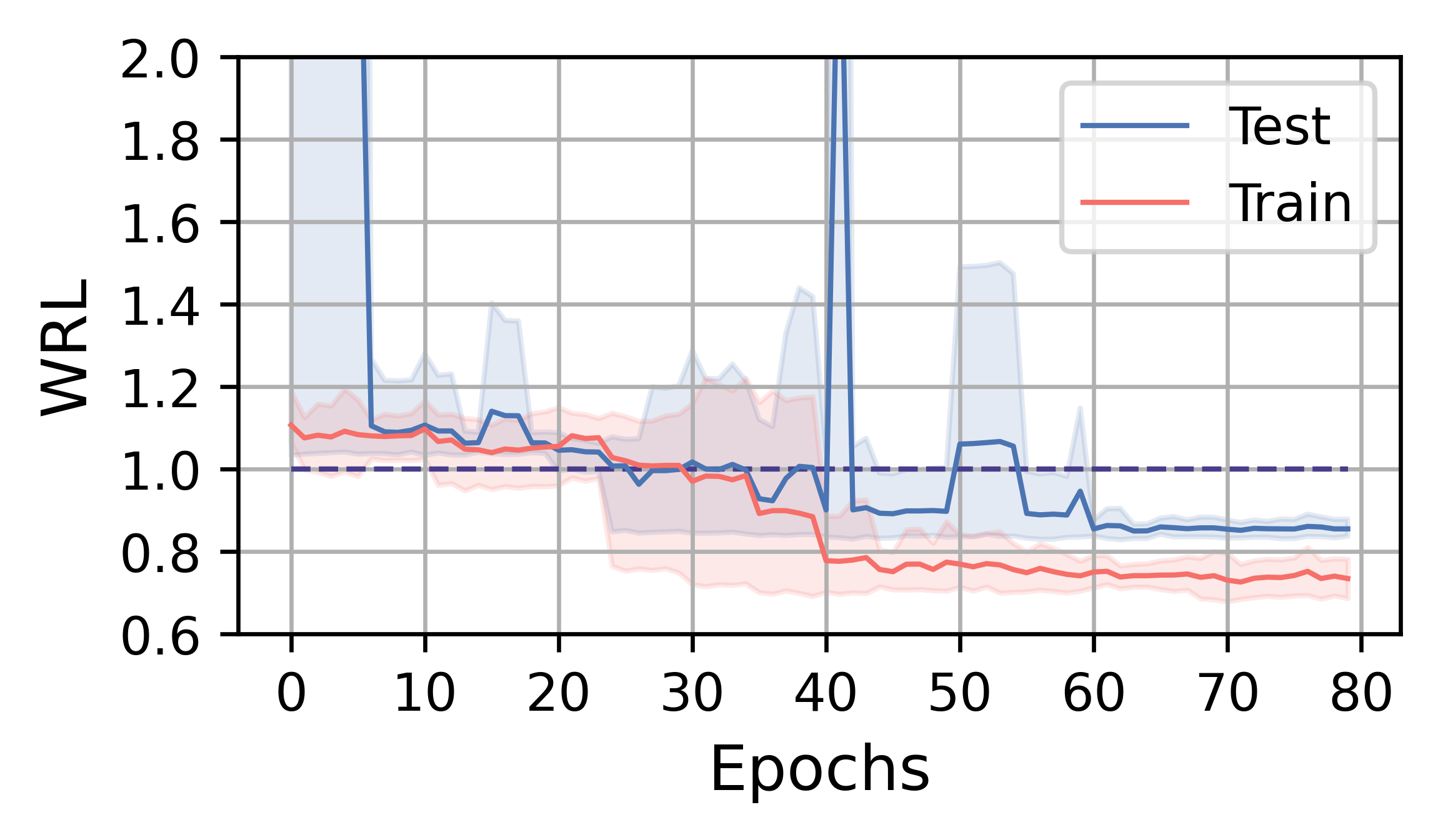
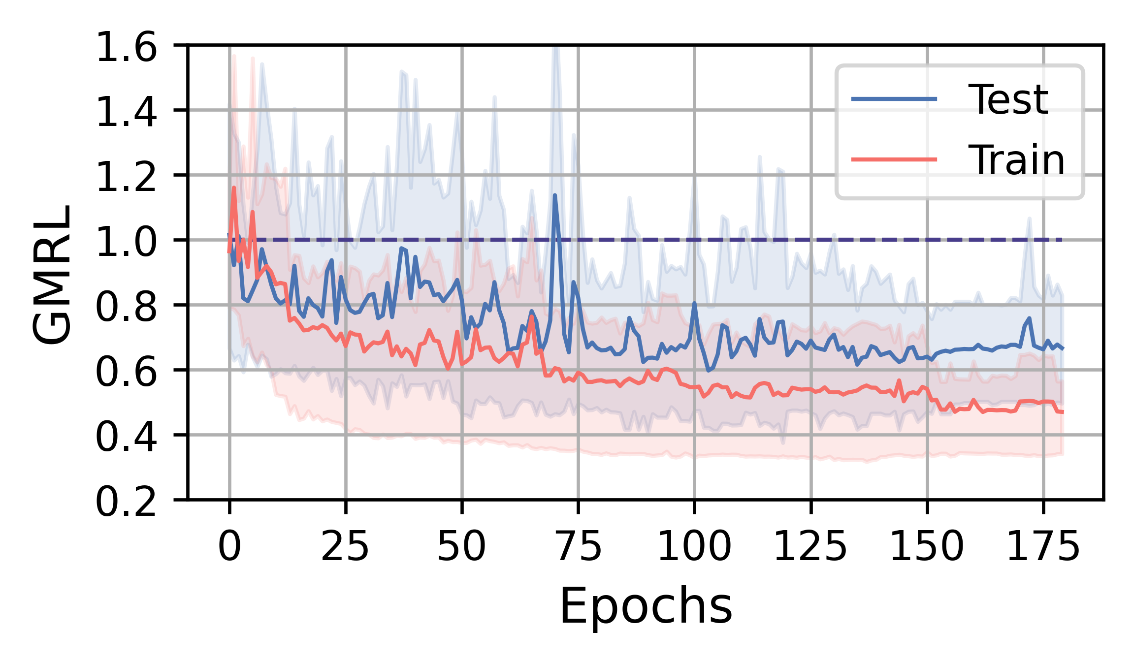
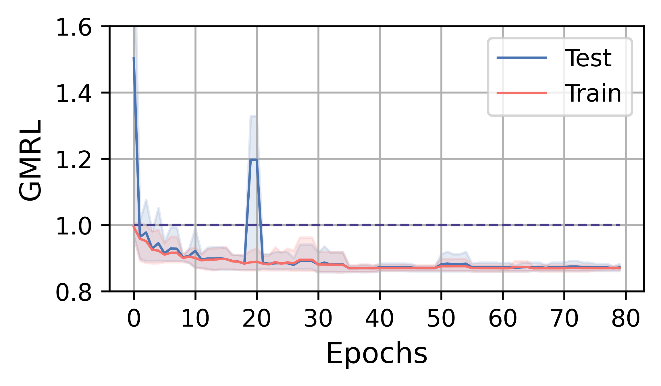
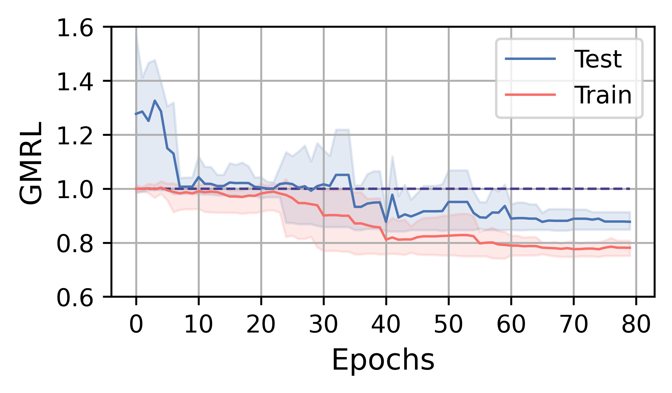
Fig. 4 illustrates the training curves of FOSS on JOB, TPC-DS, and STACK. The solid red line represents the average change in metrics over five runs on the training workload, while the blue line indicates the average change in metrics on the testing workload. The shaded area indicates the range between the minimum and maximum values. The line at 1.0 indicates the performance of the expert optimizer. Benefiting from the assurance provided by the original plans, FOSS can swiftly demonstrate its optimization effects and surpass the performance of expert optimizer.

On the JOB workload, the complexity of queries and data distribution allows FOSS to have more room for optimization. After about 8 hours of training, FOSS achieves convergence, ultimately saving $64\%$ of the latency on the testing workload relative to expert optimizer. A steady decrease on the GMRL curve until convergence to $0.64$ on the testing workload demonstrates FOSS’s ability to optimize the majority of original plans and achieve high performance. On the training workload, FOSS shows a similar convergence trend, indicating its good generalization.

On the TPC-DS and STACK workloads, FOSS occasionally encounters catastrophic plans during the training process, leading to sudden increases in WRL and GMRL. However, it can avoid these plans as training progresses, eventually converging and achieving relatively good results. Due to their simpler workload, their training processes converge in 1-3 hours and have low tail variance.

VI-B2 Performance Comparison

TABLE I: The performance of various methods and training time on different workloads.

Methods	WRL, train			GMRL, train			WRL, test			GMRL, test			Training time (hours)
	JOB	TPC-DS	STACK	JOB	TPC-DS	STACK	JOB	TPC-DS	STACK	JOB	TPC-DS	STACK	JOB	TPC-DS	STACK
PostgreSQL	1.00	1.00	1.00	1.00	1.00	1.00	1.00	1.00	1.00	1.00	1.00	1.00	/	/	/
Bao	0.22	0.78	1.58	0.54	0.96	1.18	0.44	0.78	1.37	0.84	0.95	1.78	3.35	1.32	3.03
Balsa	0.19	1.79	NA	0.62	1.98	NA	0.45	1.86	NA	1.25	2.08	NA	12.18	10.58	TLE
HybridQO	0.61	0.95	1.43	0.71	1.07	1.40	0.51	0.92	0.86	0.75	1.04	1.01	3.51	0.52	1.58
FOSS	0.17	0.78	0.73	0.48	0.87	0.78	0.36	0.77	0.85	0.64	0.87	0.87	8.09	1.55	2.31

In this subsection, we compare the performance of FOSS with the SOTA methods. We ensure that all methods are evaluated after convergence. Notably, Balsa’s training on STACK is hindered by catastrophic plans generated during the initial phase, preventing it from completing within a reasonable timeframe.

As described in Fig. 3, despite the left-deep restriction, FOSS consistently outperforms or matches the other three methods for both training and testing workloads. FOSS outperforms Bao, HybridQO, and Balsa with average speedups of 1.48×, 2.26×, and 1.71× on training workloads, and 1.28×, 1.21×, and 1.84× on testing workloads, respectively.

As shown in Table I, FOSS not only outperforms other methods at the workload total latency but also exhibits superior performance in GMRL metrics. Worth mentioning is the performance on the JOB workload, where Bao and Balsa exhibit a relatively small difference compared to FOSS in WRL, but a more significant gap emerges in GMRL. This discrepancy arises from FOSS efficiently interacting with the simulated environment, allowing for more exploration compared to Balsa. Compared to Bao, FOSS employs finer-grained optimization, resulting in a higher likelihood of generating better plans. These factors enable FOSS to surpass the expert optimizer across a broader range of queries, indicating its stronger optimization capabilities. This will be further confirmed in VI-B4. However, these advantages come with an associated cost, leading to relatively longer training time on the JOB compared to HybridQO and Bao. Nevertheless, in comparison to Balsa, another MDP-based method, FOSS exhibits a significant reduction in training time. While on STACK and TPC-DS, the training time difference among FOSS, Bao, and HybridQO is not pronounced and is much less than that of Balsa, FOSS surpasses all other methods, demonstrating the superiority of our approach.

VI-B3 Optimization Time Comparison

Figure 5: Optimization time of various optimizers.

Figure 5: Optimization time of various optimizers.

Figure 6: Steps distribution for known best plans under different maxsteps settings.

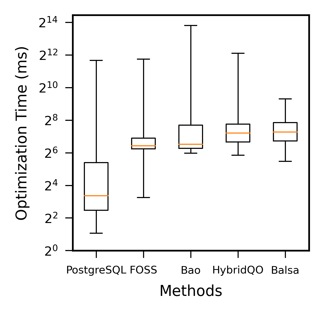
We compare the optimization time of various optimizers on the entire JOB benchmark, which is the time from the input of SQL to the generation of the execution plan. As depicted in Fig. 6, we represent the comparative results using box plots. In contrast to PostgreSQL, learned-based optimizers often require longer optimization time due to operations like model inference and plan encoding. However, the overhead is negligible compared to the time saved in execution. Among these learned-based optimizers, FOSS has the smallest 25th percentile, 50th percentile, and 75th percentile of optimization time, and its distribution is relatively concentrated. Most of its optimization time is spent on obtaining the original plan and plan encoding. Excessive reliance on the expert optimizer results in long optimization time for Bao and HybridQO. Additionally, Balsa, characterized by a lengthy average decision sequence and a wide range of plan exploration strategies, also performs poorly in terms of optimization time.

Figure 7: Ranking time savings ratios for known best plans.

VI-B4 Known Best Plan Comparison

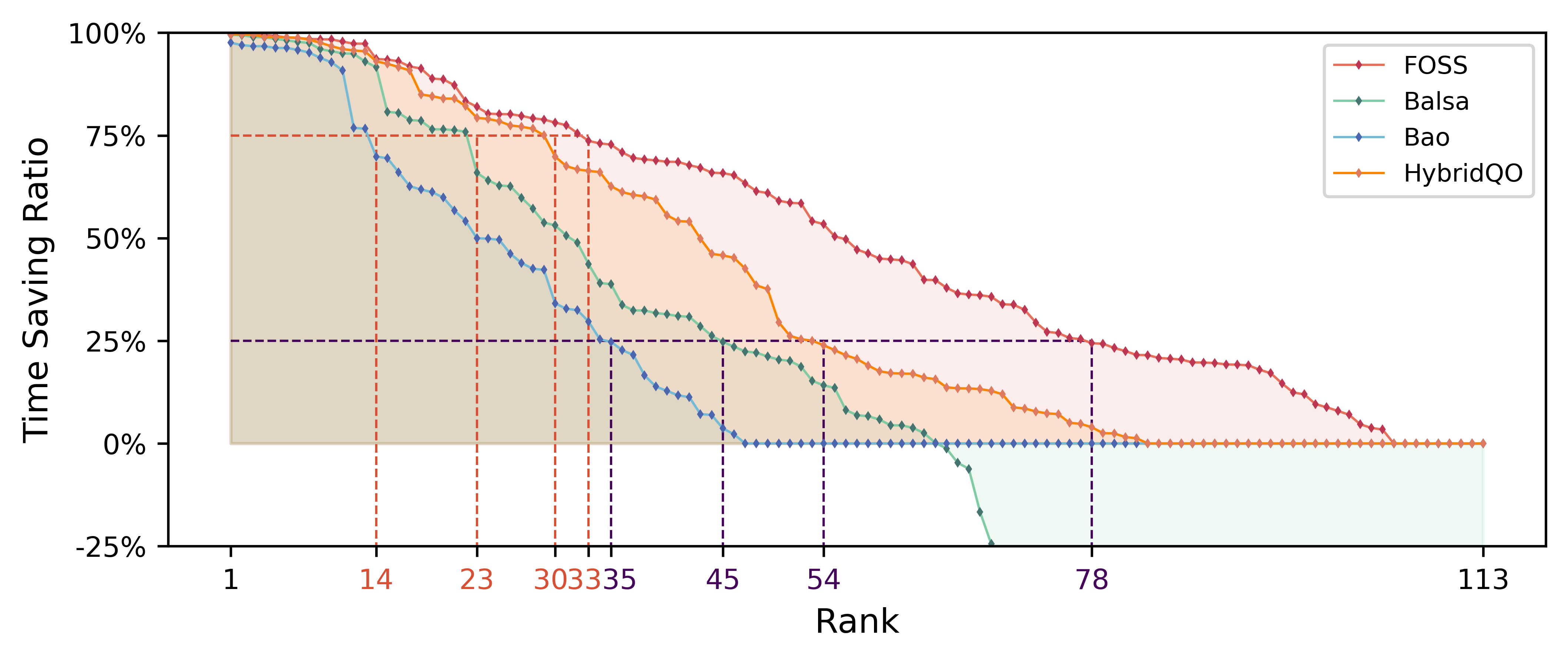
In this subsection, we analyze the optimization upper bounds of each learned-based query optimizer. We conduct five runs for each method on the entire JOB workload. From all the results, we acquire the known best plan (i.e., the one with the lowest execution latency) on each query for each method. The comparison results are shown in Fig. 7.

It illustrates the time savings ratios of the learned-based methods relative to expert optimizer in terms of known best plans. Overall, FOSS comprehensively outperforms the other three methods, surpassing the expert optimizer on a broader range of queries at each percentage point. Specially, FOSS, HybridQO, Balsa, and Bao achieve at least a $25\%$ time savings on 78, 54, 45, and 35 queries, respectively. They each save at least $75\%$ of the time on 33, 30, 23, and 14 queries, respectively. Additionally, due to the limited plan search space of Bao, it generates better-performance plans than expert optimizer across a minimal range of queries. Balsa, lacking assurance from the original plan, generates plans with poorer-performance than expert optimizer on many queries.

VI-C Analysis of design choices

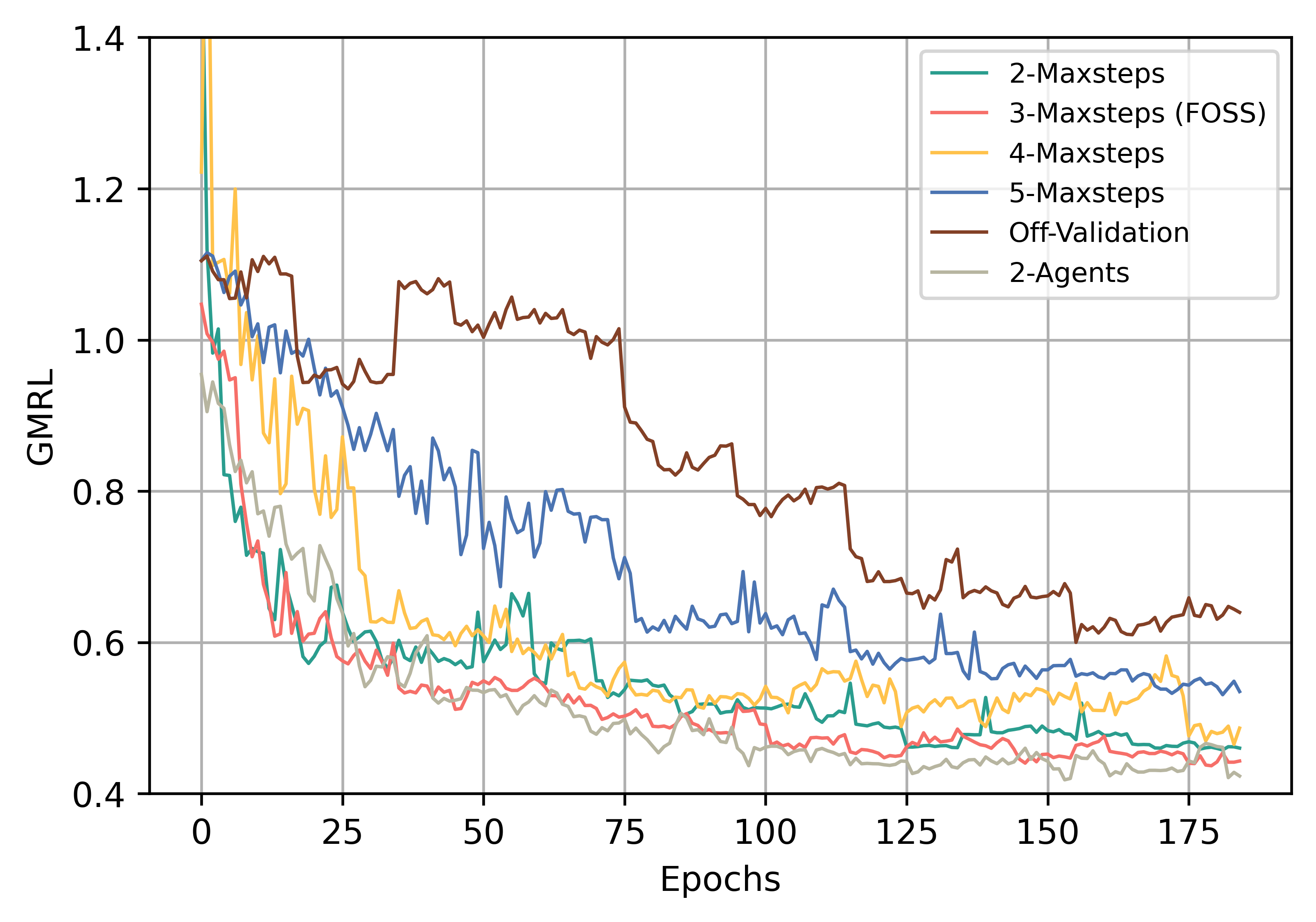
In this subsection, we analyze design choices in FOSS by individually replacing each component with alternatives. We test their performances on the entire JOB workload, using GMRL as the metric for evaluation, and consider training time and average plan optimization time for practical insights. Table II presents our comparison results and Fig. 8 illustrates the variation of GMRL during the training process.

Figure 8: GMRL variation curves under different configurations.

TABLE II: Different Configurations Comparison Results.

Experiments	Training time	Optimization Time	GMRL
	(hours)	(milliseconds)
2-Maxsteps	8.52	152.95	0.46
3-Maxsteps (FOSS)	9.23	170.57	0.44
4-Maxsteps	11.24	178.18	0.48
5-Maxsteps	15.21	190.43	0.53
Off-Simulated	48.01	171.12	0.65
Off-Validation	7.90	173.82	0.62
2-Agents	14.21	202.25	0.42

VI-C1 Determination of Maxsteps

Larger $maxsteps$ implies that FOSS can explore more diverse plans through the modifications of longer sequences to the original plan. However, it also makes the training of FOSS more challenging. We set $maxsteps$ to 2, 3, 4, and 5, respectively, and compare their performances. As described in Table II, with an increase in $maxsteps$, the optimization time grows due to the consideration of more plans. Concurrently, training time gradually increases as the plan search space expands, and the number of plans to be executed grows. As illustrated in Fig. 8, when $maxsteps$ is set to 3, FOSS achieves the best performance with the minimum GMRL.

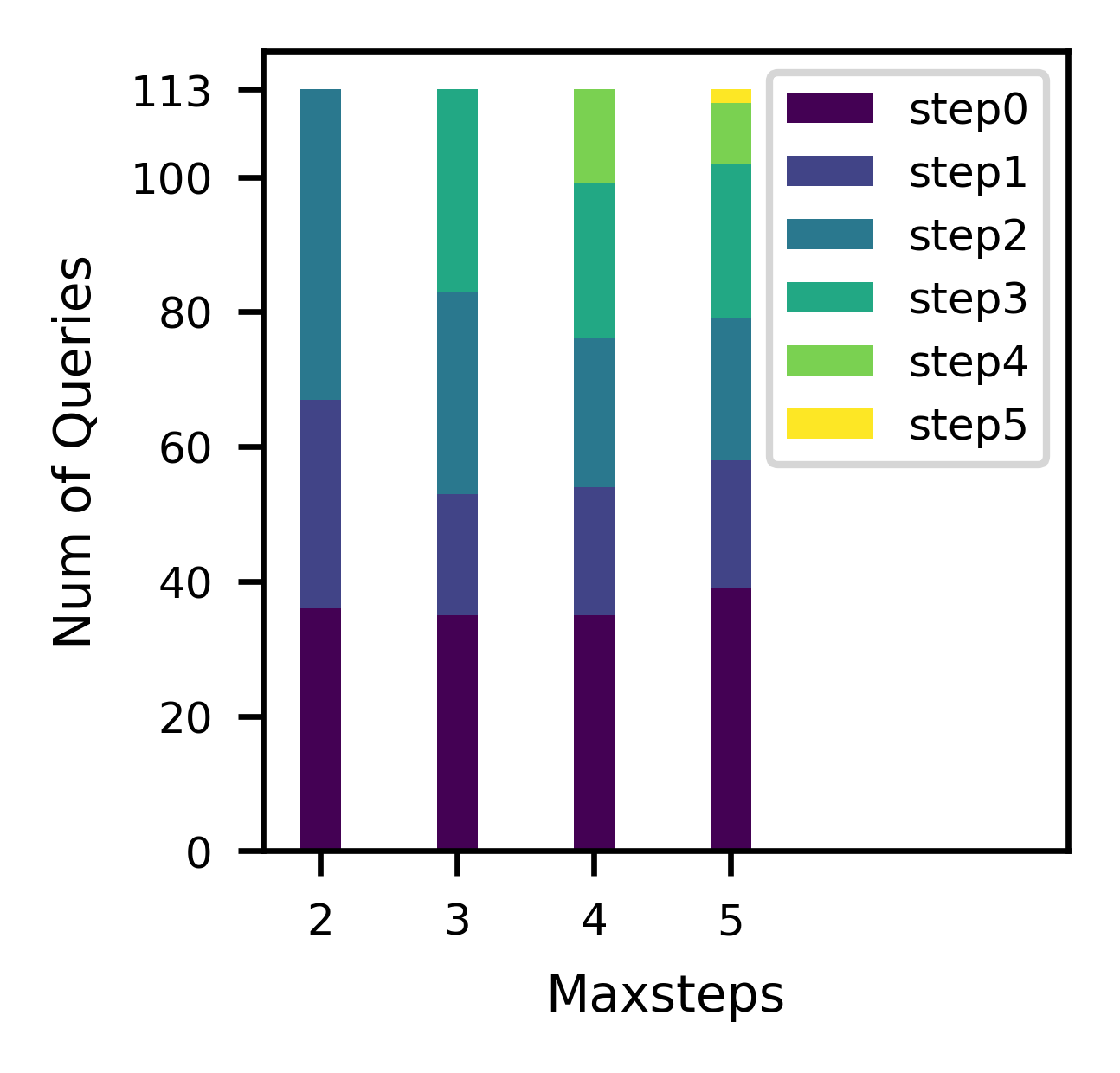
For a more in-depth comparison, as described in Fig. 6, we analyze the distribution of step status for known best plan, where step0 plans refers to the original plans, and stepN plans refers to plans that take $N$ steps from the original plans. In the bar for $2-maxsteps$, there is a significant number of step2 plans. It suggests that $2-maxsteps$ may be insufficient. In the bar for $5-maxsteps$, the proportion of step4 and step5 plans is relatively small. Despite spending nearly twice the training time of $2-maxsteps$, $5-maxsteps$ yields the lowest GMRL. This is because as $maxsteps$ increases, the longer action sequences complicates the agent’s exploration and makes it more challenging for the ${\theta }_{adv}$ to select a good plan from candidate plans. As demonstrated by the other two results, FOSS always yields effective plans within 1-3 steps. Considering both training complexity and experimental effectiveness, we set the $maxsteps$ to 3.

VI-C2 Effect of Simulated Environment

To illustrate the effect of the simulated environment, we disable it in FOSS. It allows the agent to interact only with the real environment. Due to the extensive queries executed in the real environment, it significantly prolong the training time. To make training more feasible, we have to reduce the query number for each agent update to 200. After 48 hours of training, despite benefiting from more reliable rewards feedback, its performance remains unsatisfactory. Its final GMRL is 0.63, which is significantly poorer than FOSS. The inadequacy can be ascribed to the insufficient exploration. It indicates the effectiveness of the simulated environment.

VI-C3 Effect of Validation Phase

We deploy FOSS without the validation of estimated optimal plans. As described in Table II, it reduces training time but diminishes the performance. As shown in Fig. 8, its GMRL decreases slowly with training progress, even performing worse than the expert optimizer in the early stages of training. The absence of the validation phase reduces diversity in ${\theta }_{adv}$ training data and prevents timely error alleviation, resulting in the accumulation of errors during DRL training.

VI-C4 Training with Muti-Agents

To enhance the robustness of FOSS, we also incorporate a switch for multi-agents. FOSS can initialize $m$ agents with different strategies (e.g., different discount factors). In training mode, they individually interact with the real environment, generating execution latency data pool. These data are then integrated into a new execution buffer and employed to train the ${\theta }_{adv}$. Subsequently, they interact with the simulated environment to generate simulated experiences and concurrently update themselves. In inference mode, for a given query, $m$ agents independently generate candidate plans, utilize ${\theta }_{adv}$ to select the best plan, and the ultimately optimal plan is chosen from the $m$ best plans using ${\theta }_{adv}$.

We deploy FOSS with 2 agents. It demonstrates better performance than FOSS with 1 agent (Table II) and requires fewer epochs for convergence (Fig. 8). This can be attributed to the strategy of multi-agents, which not only enriches the diversity of training data for ${\theta }_{adv}$ but also generates a more diverse set of high-quality candidate plans. However, due to our serialization configuration, it incurs more training time than FOSS with 1 agent. If computational resources are ample, we recommend deploying FOSS with multi-agents in parallel.

VII Related Work

Learned Query Optimizer. In recent years, various learned query optimizers have been proposed. Some works [4, 5, 7, 6, 10, 8, 9] model the plan generation process as MDP. Their primary goal is to train a learned value network to guide the bottom-up generation of more latency-effective plans. However, this method incurs high training costs due to its inefficient plan search, limiting its practicality. Other works [12, 26, 13, 27] aim to steer the plan generation in traditional optimizer using hint sets. This method is more practical, but its coarse-grained hint optimization approach cannot perform fine-grained optimization of join order and physical operators, limiting the plan search space. FOSS strikes a balance between these two approaches, offering practicality while still exploring a significant portion of the optimization possibilities.

Recently, the works [28, 29] build upon the foundation laid by Bao[12], employing hint sets similar to Bao. They focus on making the selection of candidate hint set more intelligent rather than relying solely on expert knowledge. Their work contributes positively to the advancement of plan-steerer.
Reinforcement Learning. Reinforcement learning can be divided into model-free RL and model-based RL. The former have experienced rapid development in the past few years, with many classic algorithms [30, 31, 21, 32, 33] being proposed and demonstrating excellent performance in various fields [34, 35, 36, 37]. However, model-free RL with high sample complexity are hard to be directly applied in real-world tasks, where trial-and-errors can be highly costly [18]. As a result, some scholars are dedicated to building simulated environment models to interact more efficiently with agents. FOSS follows the Dyna-style [38] method, using the learned environment model to generate more simulated experience data for the agent. In addition to the mentioned approach, in many model-based RL scenarios, the simulated environment models are differentiable. This enables policy learning through differential planning and value gradient methods [18].
Reinforcement Learning From Human Feedback. Reinforcement learning from human feedback (RLHF) is a technique employed for training AI systems to align with human goals. RLHF has emerged as the primary method for fine-tuning SOTA large language models [39]. The standard methodology for RLHF used today was introduced by [40] in 2017. Its framework is similar to FOSS, requiring feedback from external comparisons of two samples to train a reward model. This reward model is then used to train traditional RL, which is policy optimization. The key difference is that RLHF receives feedback from humans, making sample labeling more challenging due to human subjectivity, whereas FOSS obtains feedback from DBMS’s real execution.

VIII conclusion

We introduce FOSS, a novel DRL-based query optimization system. Starting from the original plans generated by traditional optimizer, the planner of FOSS experiments with the optimization of these plans through step-by-step modifications, which results in candidate plans. We design an asymmetric advantage model to serve as a selector, choosing the optimal plan from the candidate plans. Furthermore, to enhance training efficiency, we employ the asymmetric advantage model as a reward indicator and integrate it with a traditional optimizer to build a simulated environment. With the simulated environment, FOSS can enhance its optimization ability through self-bootstrapping.

To our knowledge, FOSS is the pioneering learned-based query optimizer that achieves better-performance plans through fine-grained modifications to the original plans and employs a learned model for accelerating the training process of DRL. We believe that FOSS opens up a new path for query optimization and deserves further exploration.

References

- [1] P. G. Selinger, M. M. Astrahan, D. D. Chamberlin, R. A. Lorie, and T. G. Price, “Access path selection in a relational database management system,” in Proceedings of the 1979 ACM SIGMOD International Conference on Management of Data, ser. SIGMOD ’79. New York, NY, USA: Association for Computing Machinery, 1979, p. 23–34. [Online]. Available: https://doi.org/10.1145/582095.582099
- [2] V. Leis, A. Gubichev, A. Mirchev, P. Boncz, A. Kemper, and T. Neumann, “How good are query optimizers, really?” Proc. VLDB Endow., vol. 9, no. 3, p. 204–215, nov 2015. [Online]. Available: https://doi.org/10.14778/2850583.2850594
- [3] X. Zhou, C. Chai, G. Li, and J. Sun, “Database meets artificial intelligence: A survey,” IEEE Transactions on Knowledge and Data Engineering, vol. 34, no. 3, pp. 1096–1116, 2022.
- [4] R. Marcus and O. Papaemmanouil, “Deep reinforcement learning for join order enumeration,” in Proceedings of the First International Workshop on Exploiting Artificial Intelligence Techniques for Data Management, ser. aiDM’18. New York, NY, USA: Association for Computing Machinery, 2018. [Online]. Available: https://doi.org/10.1145/3211954.3211957
- [5] S. Krishnan, Z. Yang, K. Goldberg, J. M. Hellerstein, and I. Stoica, “Learning to optimize join queries with deep reinforcement learning,” ArXiv, vol. abs/1808.03196, 2018.
- [6] X. Yu, G. Li, C. Chai, and N. Tang, “Reinforcement learning with tree-lstm for join order selection,” in 2020 IEEE 36th International Conference on Data Engineering (ICDE), 2020, pp. 1297–1308.
- [7] R. Marcus, P. Negi, H. Mao, C. Zhang, M. Alizadeh, T. Kraska, O. Papaemmanouil, and N. Tatbul, “Neo: A learned query optimizer,” Proc. VLDB Endow., vol. 12, no. 11, p. 1705–1718, jul 2019. [Online]. Available: https://doi.org/10.14778/3342263.3342644
- [8] Z. Yang, W.-L. Chiang, S. Luan, G. Mittal, M. Luo, and I. Stoica, “Balsa: Learning a query optimizer without expert demonstrations,” in Proceedings of the 2022 International Conference on Management of Data, ser. SIGMOD/PODS ’22. New York, NY, USA: Association for Computing Machinery, 2022, pp. 931–944. [Online]. Available: https://doi.org/10.1145/3514221.3517885
- [9] T. Chen, J. Gao, H. Chen, and Y. Tu, “Loger: A learned optimizer towards generating efficient and robust query execution plans,” Proc. VLDB Endow., vol. 16, pp. 1777–1789, 2023.
- [10] J. Chen, G. Ye, Y. Zhao, S. Liu, L. Deng, X. Chen, R. Zhou, and K. Zheng, “Efficient join order selection learning with graph-based representation,” in Proceedings of the 28th ACM SIGKDD Conference on Knowledge Discovery and Data Mining, ser. KDD ’22. New York, NY, USA: Association for Computing Machinery, 2022, p. 97–107. [Online]. Available: https://doi.org/10.1145/3534678.3539303
- [11] M. A. Riedmiller, R. Hafner, T. Lampe, M. Neunert, J. Degrave, T. V. de Wiele, V. Mnih, N. M. O. Heess, and J. T. Springenberg, “Learning by playing - solving sparse reward tasks from scratch,” ArXiv, vol. abs/1802.10567, 2018. [Online]. Available: https://api.semanticscholar.org/CorpusID:3562704
- [12] R. Marcus, P. Negi, H. Mao, N. Tatbul, M. Alizadeh, and T. Kraska, “Bao: Making learned query optimization practical,” in Proceedings of the 2021 International Conference on Management of Data, ser. SIGMOD ’21. New York, NY, USA: Association for Computing Machinery, 2021, p. 1275–1288. [Online]. Available: https://doi.org/10.1145/3448016.3452838
- [13] R. Zhu, W. Chen, B. Ding, X. Chen, A. Pfadler, Z. Wu, and J. Zhou, “Lero: A learning-to-rank query optimizer,” Proc. VLDB Endow., vol. 16, no. 6, p. 1466–1479, apr 2023. [Online]. Available: https://doi.org/10.14778/3583140.3583160
- [14] X. Yu, C. Chai, G. Li, and J. Liu, “Cost-based or learning-based? a hybrid query optimizer for query plan selection,” Proc. VLDB Endow., vol. 15, no. 13, p. 3924–3936, sep 2022. [Online]. Available: https://doi.org/10.14778/3565838.3565846
- [15] A. Vaswani, N. M. Shazeer, N. Parmar, J. Uszkoreit, L. Jones, A. N. Gomez, L. Kaiser, and I. Polosukhin, “Attention is all you need,” in Neural Information Processing Systems, 2017. [Online]. Available: https://api.semanticscholar.org/CorpusID:13756489
- [16] Y. Zhao, G. Cong, J. Shi, and C. Miao, “Queryformer: A tree transformer model for query plan representation,” Proc. VLDB Endow., vol. 15, no. 8, p. 1658–1670, apr 2022. [Online]. Available: https://doi.org/10.14778/3529337.3529349
- [17] E. B. Baruch, T. Ridnik, N. Zamir, A. Noy, I. Friedman, M. Protter, and L. Zelnik-Manor, “Asymmetric loss for multi-label classification,” 2021 IEEE/CVF International Conference on Computer Vision (ICCV), pp. 82–91, 2020. [Online]. Available: https://api.semanticscholar.org/CorpusID:221995872
- [18] F. Luo, T. Xu, H. Lai, X.-H. Chen, W. Zhang, and Y. Yu, “A survey on model-based reinforcement learning,” ArXiv, vol. abs/2206.09328, 2022.
- [19] T. M. Moerland, J. Broekens, and C. M. Jonker, “Model-based reinforcement learning: A survey,” Found. Trends Mach. Learn., vol. 16, pp. 1–118, 2020.
- [20] “Ray,” https://www.ray.io, 2023.
- [21] J. Schulman, F. Wolski, P. Dhariwal, A. Radford, and O. Klimov, “Proximal policy optimization algorithms,” ArXiv, vol. abs/1707.06347, 2017.
- [22] M. Poess, B. Smith, L. Kollar, and P. Larson, “Tpc-ds, taking decision support benchmarking to the next level,” in Proceedings of the 2002 ACM SIGMOD International Conference on Management of Data, ser. SIGMOD ’02. New York, NY, USA: Association for Computing Machinery, 2002, p. 582–587. [Online]. Available: https://doi.org/10.1145/564691.564759
- [23] “Bao project,” https://rmarcus.info/bao_docs/, 2021.
- [24] “Balsa project,” https://github.com/balsa-project/balsa, 2022.
- [25] “Hybridqo project,” https://github.com/yxfish13/HyperQO, 2022.
- [26] L. Sun, T. Ji, C. Li, and H. Chen, “Deepo: A learned query optimizer,” Proceedings of the 2022 International Conference on Management of Data, 2022. [Online]. Available: https://api.semanticscholar.org/CorpusID:249579130
- [27] X. Chen, H. Chen, Z. Liang, S. Liu, J. Wang, K. Zeng, H. Su, and K. Zheng, “Leon: A new framework for ml-aided query optimization,” Proc. VLDB Endow., vol. 16, pp. 2261–2273, 2023. [Online]. Available: https://api.semanticscholar.org/CorpusID:259246460
- [28] C. Anneser, N. Tatbul, D. Cohen, Z. Xu, N. P. Laptev, R. Marcus, P. Pandian, and R. M. AutoSteer, “Autosteer: Learned query optimization for any sql database,” Proceedings of the VLDB Endowment, 2023. [Online]. Available: https://api.semanticscholar.org/CorpusID:261259493
- [29] L. Woltmann, J. Thiessat, C. Hartmann, D. Habich, and W. Lehner, “Fastgres: Making learned query optimizer hinting effective,” Proceedings of the VLDB Endowment, 2023. [Online]. Available: https://api.semanticscholar.org/CorpusID:261199199
- [30] V. Mnih, K. Kavukcuoglu, D. Silver, A. Graves, I. Antonoglou, D. Wierstra, and M. A. Riedmiller, “Playing atari with deep reinforcement learning,” ArXiv, vol. abs/1312.5602, 2013.
- [31] H. Van Hasselt, A. Guez, and D. Silver, “Deep reinforcement learning with double q-learning,” in Proceedings of the AAAI conference on artificial intelligence, vol. 30, no. 1, 2016.
- [32] V. Mnih, A. P. Badia, M. Mirza, A. Graves, T. Harley, T. P. Lillicrap, D. Silver, and K. Kavukcuoglu, “Asynchronous methods for deep reinforcement learning,” in Proceedings of the 33rd International Conference on International Conference on Machine Learning - Volume 48, ser. ICML’16. JMLR.org, 2016, p. 1928–1937.
- [33] T. Haarnoja, A. Zhou, P. Abbeel, and S. Levine, “Soft actor-critic: Off-policy maximum entropy deep reinforcement learning with a stochastic actor,” International Conference on Machine Learning (ICML), 2018.
- [34] V. Mnih, K. Kavukcuoglu, D. Silver, A. A. Rusu, J. Veness, M. G. Bellemare, A. Graves, M. A. Riedmiller, A. K. Fidjeland, G. Ostrovski, S. Petersen, C. Beattie, A. Sadik, I. Antonoglou, H. King, D. Kumaran, D. Wierstra, S. Legg, and D. Hassabis, “Human-level control through deep reinforcement learning,” Nature, vol. 518, pp. 529–533, 2015.
- [35] D. Silver, A. Huang, C. J. Maddison, A. Guez, L. Sifre, G. van den Driessche, J. Schrittwieser, I. Antonoglou, V. Panneershelvam, M. Lanctot, S. Dieleman, D. Grewe, J. Nham, N. Kalchbrenner, I. Sutskever, T. P. Lillicrap, M. Leach, K. Kavukcuoglu, T. Graepel, and D. Hassabis, “Mastering the game of go with deep neural networks and tree search,” Nature, vol. 529, pp. 484–489, 2016.
- [36] D. Silver, J. Schrittwieser, K. Simonyan, I. Antonoglou, A. Huang, A. Guez, T. Hubert, L. baker, M. Lai, A. Bolton, Y. Chen, T. P. Lillicrap, F. Hui, L. Sifre, G. van den Driessche, T. Graepel, and D. Hassabis, “Mastering the game of go without human knowledge,” Nature, vol. 550, pp. 354–359, 2017.
- [37] S. Levine, C. Finn, T. Darrell, and P. Abbeel, “End-to-end training of deep visuomotor policies,” J. Mach. Learn. Res., vol. 17, pp. 39:1–39:40, 2015.
- [38] R. S. Sutton, “Dyna, an integrated architecture for learning, planning, and reacting,” SIGART Bull., vol. 2, no. 4, p. 160–163, jul 1991. [Online]. Available: https://doi.org/10.1145/122344.122377
- [39] S. Casper, X. Davies, C. Shi, T. K. Gilbert, J. Scheurer, J. Rando, R. Freedman, T. Korbak, D. Lindner, P. Freire, T. Wang, S. Marks, C.-R. Ségerie, M. Carroll, A. Peng, P. J. Christoffersen, M. Damani, S. Slocum, U. Anwar, A. Siththaranjan, M. Nadeau, E. J. Michaud, J. Pfau, D. Krasheninnikov, X. Chen, L. L. di Langosco, P. Hase, E. Biyik, A. D. Dragan, D. Krueger, D. Sadigh, and D. Hadfield-Menell, “Open problems and fundamental limitations of reinforcement learning from human feedback,” ArXiv, vol. abs/2307.15217, 2023. [Online]. Available: https://api.semanticscholar.org/CorpusID:260316010
- [40] P. F. Christiano, J. Leike, T. B. Brown, M. Martic, S. Legg, and D. Amodei, “Deep reinforcement learning from human preferences,” ArXiv, vol. abs/1706.03741, 2017. [Online]. Available: https://api.semanticscholar.org/CorpusID:4787508