Multi-View 3D Instance Segmentation of Structural Anomalies
for Enhanced Structural Inspection of Concrete Bridges
Abstract
For effective structural damage assessment, the instances of damages need to be localized in the world of a 3D model. Due to a lack of data, the detection of structural anomalies can currently not be directly learned and performed in 3D space. In this work, a three-stage approach is presented, which uses the good performance of detection models on image level to segment instances of anomalies in the 3D space. In the detection stage, semantic segmentation predictions are produced on image level. The mapping stage transfers the image-level prediction onto the respective point cloud. In the extraction stage, 3D anomaly instances are extracted from the segmented point cloud. Cloud contraction is used to transform cracks into their medial axis representation. For areal anomalies the bounding polygon is extracted by means of alpha shapes. The approach covers the classes crack, spalling, and corrosion and the three image-level segmentation models TopoCrack pantoja2022topo , nnU-Net benz2023ai , and DetectionHMA benz2022image are compared. Granted a localization tolerance of 4 cm, IoUs of over 90% can be achieved for crack and corrosion and 41% for spalling, which appears to be a specifically challenging class. Detection on instance-level measured in is about 45% for crack and spalling and 73% for corrosion.
keywords:
Structural Condition Assessment, Structural Inspection, Structural Health Monitoring (SHM), Deep Learning, Crack Detection, 3D Anomaly Detection[inst1]organization=Computer Vision in Engineering, Bauhaus-Universität,addressline=Schwanseestraße 143, city=Weimar, postcode=99427, state=Thuringia, country=Germany
1 Introduction
The importance of structural health monitoring (SHM) for modern societies is undisputable. It ensures critical infrastructure to stay operational or to be, if necessary, renewed in a timely and systematic manner. Thereby, it contributes to the safe and enduring usage of critical infrastructure, a crucial component in the functioning of modern societies. Transportation routes rely on infrastructure to enable good’s delivery and individual mobility. In particular, bridges are used to shorten routes or bypass rough terrain, which sometimes renders them the only viable connection between two locations. The exposure to weathering and diverse forces makes bridges especially vulnerable to degradation and unforeseeable collapse often has catastrophic dimensions. The regular inspection of bridges is, thus, of high societal benefit, while posing substantial challenges for men and machines involved.
The availability and utilization of new technologies has led to a growth of research activity on automating structure inspection. Especially, the advent of more versatile image acquisition platforms, such as UAS (unmanned aircraft system, aka drones), and advanced data algorithms, such as machine learning, have boosted research and engineering in the field. With ever more and better technologies and data at hand, the gap to real-world application is gradually about to close.
As a consequence, research on the image-based recognition of structural anomalies on the surface of critical infrastructure is rapidly growing. While current work focuses on detecting cracks and other anomalies on image level, the transfer of this information into the 3D space of point clouds is underexplored. The severity of an anomaly, however, substantially depends on the place of its occurrence on the structure. The proper location of an anomaly on the structure is hardly accessible with reference to the images alone. Thus, the extension of the detection of structural anomalies beyond the image level forms the subject of this work.
For effective structure inspection in 3D, the transfer of detection results from image level to the 3D space is one key aspect. However, only the discretization of mapped results into dedicated anomaly instances in 3D enables the quantitative analysis of the their extend. Information such as the length and width of cracks or the area covered by corrosion or spalling can sustainably support the decision process of the experts involved. Furthermore, it paves the road for improved traceability, objectivity, and verifiability of the inspection criteria that determine particular decisions.
For that purpose, a workflow is here presented, that accomplishes the segmentation of instances on a 3D point cloud. It makes use of SOTA models for semantic segmentation of structural anomalies on image-level (detection stage) and projects the 2D predictions on a 3D point cloud (mapping stage) by means of point colorization. This procedure does not yield anomaly instances. Thus, the points are subsequently clustered and cracks are transformed into medial axes while bounding polygons are used to represent areal anomalies (extraction stage). The obtained anomaly instances enable the computation of additional quantitative indicators such as the crack width and length or the area and circumference of areal anomalies.
The main contributions of this work are:
-
1.
The demonstration and implementation of a fully-functional workflow for the detection, mapping, and extraction of structural anomalies in 3D point clouds.
-
2.
The introduction and application of reasonable transformations of cracks and areal anomalies into measurable 3D instances.
-
3.
A thorough evaluation and comparison of SOTA models for the proposed workflow of 3D anomaly instance segmentation on real-world data.
After the presentation of the related work, the detection workflow is explained in-depth encompassing the detection, mapping, and extraction stage. Extensive evaluation demonstrate the strengths and weaknesses of the approaches and visualizations provided a qualitative impression of the results.
2 Related Work
Three major fields of related work are identified: the detection of cracks and other structural anomalies on image level as well a approaches to 3D anomaly detection.
2.1 Crack Segmentation
mohan2018crack provide a survey on crack detection before artificial neural networks (ANN) became the dominant approach. Edge detection, morphological operations, filtering, and thresholding were among the most frequently used techniques abdel2003analysis ; oliveira2012automatic ; talab2016detection ; sinha2006automated ; salman2013pavement ; lins2016automatic ; yeum2015vision . The CrackTree approach zou2012cracktree constructs a minimum spanning tree over previously identified crack seeds. An ensemble of decision trees called CrackForest is used by shi2016automatic for crack classification.
Since 2017, artificial neural networks (ANN) have emerged as the dominant approach for crack detection. dorafshan2018comparison conducted a study comparing different training configurations of AlexNet krizhevsky2012imagenet with six edge detectors, including Sobel, LoG, and Butterworth. Experiments on the SDNET dataset dorafshan2018sdnet2018 indicated the superiority of ANN and the effectiveness of transfer learning. Other approaches, proposed by zhang2016road ; chen2017nb ; cha2017deep , involve using a classification CNN combined with a sliding window to process larger images and/or improve localization. yang2018automatic popularized the transition to fully-convolutional networks (FCN) long2015fully for crack segmentation. Based on SegNet badrinarayanan2017segnet , DeepCrackZ was designed zou2018deepcrack : a separate fusion logic with individual, scale-wise losses supports preserving thin structures. The conceptually similar approach DeepCrackL222DeepCrackZ and DeepCrackL are used for disambiguation since both were originally named ‘DeepCrack’. is suggested by liu2019deepcrack . In the style of deeply-supervised nets (DSN) lee2015deeply , losses are computed for intermediate side-outputs to make use of fine details and anti-noise capabilities alike. The outputs undergo post-processing with guided filtering (GF) he2012guided and conditional random fields (CRF) zheng2015conditional . A U-Net ronneberger2015u with focal loss lin2017focal is reported to perform superiorly compared to a simpler FCN design liu2019computer . yang2019feature propose the feature pyramid and hierarchical boosting network (FPHBN). It extends holistically-nested edge detection (HED) xie2015holistically by a feature pyramid module to incorporate and propagate context information to lower levels. The hierarchical boosting supports the inter-level communication within the FPHBN. liu2021crackformer develop CrackFormer, which is a transformer-based approach to crack segmentation. For that purpose, the convolutional layers of VGG simonyan2014very are replaced by a self-attention logic. To increase the crack sharpness, a scaling-attention block is suggested. benz2022image propose a re-trained version of the hierarchical multi-scale attention network by tao2020hierarchical called HMA, which mitigates the scale sensitivity of cracks. The results are aggregated based on the attention to cracks on different levels of scales. In order to preserve the continuity of cracks, pantoja2022topo suggest TOPO loss, which uses maximin paths to mitigate discontinuities between cracks. An oriented bounding box approach, named CrackDet, has recently been proposed by chen2023devil . bianchi2022development and kulkarni2022crackseg9k emphasize the usefulness of transfer learning and compose smaller crack datasets into larger ones, Conglo, and CrackSeg9k. kulkarni2022crackseg9k compare a number of approaches, including Pix2Pix, SWIN, and MaskRCNN. DeepLabV3+ chen2018encoder with a ResNet-101 backbone outperformed the other methods. bianchi2022development confirm that DeepLabV3+ is an effective method for crack segmentation.
2.2 Detection of Structural Anomalies
While a multitude of datasets and approaches on crack detection has been published over the past years, interest and resources on the image-based detection of other structural anomalies has only recently picked up pace. Analogous to crack detection, the paradigm of image classification to anomaly detection was first explored. Classes such as spalling and efflorescence are featured by the CODEBRIM mundt2019meta and MCDS huthwohl2019multi datasets. A meta-learning approach for neural architecture search (NAS) on CODEBRIM is proposed by mundt2019meta , which slightly outperforms VGG- simonyan2014very and DenseNet-based huang2017densely approaches. The NAS-based model requires distinctly fewer parameters. Benchmarking and extensive hyperparameter tuning for transfer learning on these datasets is performed by flotzinger2022building .
Science 2021, a shift towards semantic segmentation for structural anomaly detection has been observed. benz2022image published the S2DS dataset with 743 images, which features anomalies such as crack, spalling, corrosion, efflorescence, and vegetation. The proposed DetectionHMA benz2022image uses attention maps over different scales to effectively exploit multi-scale information. To systematize the increasing number of datasets, bianchi2022visual surveyed published datasets for structural inspection and started an initiate to list available datasets333https://github.com/beric7/structural_inspection_main/tree/main/cataloged_review, accessed 29 Dec, 2023.. The CSSC yang2017deep dataset represent cracks and spalling. CrSpEE bai2021detecting covers the same anomalies in an ‘in the wild’ scenario, i.e. with substantial distractors (people, context, background) being present. Very recently flotzinger2024dacl10k published the dacl10k dataset which contains 10,000 images and i.a. includes the classes crack, spalling, rust, efflorescence, wetspot, rockpocket, and weathering. The corresponding challenge hosted at WACV’24 flotzinger2024dacl indicated the power of transfer learning on SOTA models for semantic segmentation such as ConvNeXt-Large liu2022convnet , EVA-02-Large fang2023eva , or Mask2Former cheng2022masked and the extensive usage of ensembles.
2.3 3D Anomaly Detection
The attention in the image-based detection of cracks and other structural anomalies in the 3D space has recently been growing. The state is premature and a lack of publicly available datasets is observed that interferes with effective model training and evaluation. For 3D anomaly detection in the industrial context, the MVTec 3D-AD dataset was published bergmann2021mvtec . The dataset features point clouds with scratches, holes, deformations, and other anomalies in ten industrially relevant categories, including cookies, carrots, dowels, and ropes. For MVTec 3D-AD, bergmann2023anomaly transfer an unsupervised student-teacher approach to 3D and infer defective point clouds from deep feature descriptors. The application context of MVTec 3D-AD differs from structural inspection by the controlled acquisition circumstances, the achieved 3D resolution, and the captured objects.
Over the last decade, a number of approaches specifically have targeted 3D structural inspection. jahanshahi2012adaptive propose a system for 3D crack detection by combining the information from multiple images making use of the depth information obtained from SfM. To spot cracks in a triangulated mesh, torok2014image make use of the deviation of normals compared to the medial axis of an element. huang2014pavement use depth information captured by a laser scanner to support image-based crack segmentation. A CNN named CrackNet is presented by zhang2017automated , which operates on depth maps for pavement cracks. A learning-based successor is proposed by zhang2018deep . Embedding features for 3D points are extracted by chen2022crackembed and used to segment crack regions in an unsupervised manner. pantoja2023damage pre-segment building facades and subsequently project cracks, that were segmented on image level, onto the 3D model.
Based on the comparatively low resolution of point clouds in real inspection scenarios, methods operating natively on point cloud level render suitable for the application case of this work. 3D anomaly detection is, thus, here approached by using the higher resolution from multiple views. Since data are currently too scarce, end-to-end training of a multi-view point cloud segmentation method is currently not feasible. Therefore, the effective performance of anomaly detection in 2D is leveraged in a multi-stage approach to effectively transform 2D results into 3D anomaly instances.
3 Data
Due to the recency of the field, no proper, labeled 3D data for structural anomaly detection is yet available to the public. Reasons for the absence of such datasets include:
- Reachability:
-
Many parts of structures are typically not reachable without greater effort. Modern image acquisition platforms such as UAS facilitate reachability, which, however, remains a challenging endeavor.
- Region of Interest:
-
The surface of structures is large and anomalies typically occur rare and punctually. The identification of relevant regions is a labor-intensive task. In that respect, it must be considered a hen’s egg problem: the goal of 3D anomaly detection is to automate this process. Dataset creation, however, first requires the manual retrieval of anomalies.
- Quality Requirements:
-
Crack detection poses challenging requirements in terms of image resolution. Acquiring overlapping images of resolution 0.15 mm with good quality by means of a moving platform (such as UAS) is a distinct challenge leading to only a few usable datasets of respective quality and resolution.
- Labeling Effort:
-
Effective labeling must include field experts, which are rarely available (or willing) for labeling data in a wider scope.
- Scalability:
-
Point clouds scale weakly for very high resolutions leading to point clouds of more than 20M points. Therefore, technical reasons currently call for point clouds of manageable size.
- Data Protection:
-
The structure maintainers do usually not want the (potentially defective) structure to be exposed to the public. Beside bringing negative publicity, the defectiveness of a structure could also be exploited for (terrorist) attacks.
- 3D Structure:
-
Usually, a large portion of a structure’s surface is planar. Only few parts exhibit non-planar areas such as corners or niches. Exploring 3D anomaly detection renders reasonable only on defective non-planar parts of the structure.
Despite the listed obstacles, a dataset was created in the context of this work. The dataset features four segments from two concrete bridges that showed anomalies suitable for 3D anomaly detection.
| Bridge B | Bridge G | ||||||||||||||||||||||||||||||||||
| Dev | Test | Dev | Test | ||||||||||||||||||||||||||||||||
|
|
|
|
|
|||||||||||||||||||||||||||||||
3.1 3D Reconstruction
Capturing 3D real-world data is a challenging task, which is typically performed by processing 2D representations and thereupon inferring the 3D Structure. While a number of methods for measuring the 3D structure of objects are available – including structured light sensors and time-of-flight (TOF) cameras (e.g. steger2018machine ) – image-based stereo reconstruction is the standard procedure in structural inspection.
The reconstruction of a static 3D scene from multiple images still follows the principles published in pollefeys2004visual : The structure-from-motion (SfM) pipeline infers the relative orientation of the views, which is subsequently used to perform multi-view stereo (MVS) yielding a dense point cloud. This procedure is implemented in the COLMAP444https://colmap.github.io/, accessed Dec 20, 2023. software schonberger2016structure ; schonberger2016pixelwise , widely used in academia and industry. Beside COLMAP, which is available under a permissive open-source license, a number of commercial products exists such as Reality Capture555https://www.capturingreality.com/, accessed Dec 20, 2023. or Agisoft Metashape666https://www.agisoft.com/, accessed Dec 20, 2023.. The latter of which was used in this work to compute a 3D point cloud and textured mesh from the captured images.
3.2 Dataset
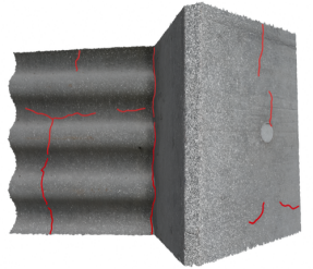
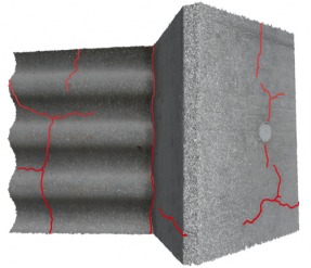
Table 1 provides an overview of the created dataset. Bridge B is a highway bridge in Germany, that shows comparatively wide cracks in the range of 0.5 to 1.0 mm. One of the bridge’s accessible piers was captured with a Sony 7r I camera being moved around the pier’s base on a tripod adjusted to two different altitudes. The second object, Bridge G, is a railway bridge showing defects of spalling and corrosion. The images were captured by means of the UAS, Intel Falcon 8+, with a Sony 7r I camera being mounted on a compatible gimbal. Four segments were extracted from the two bridges, which showed relevant anomalies at niches or corners. One segment of each bridge is used in the development set for parameter tuning, the other two segments form the test set. For a visual impression of the two test segments, please refer to Figure 4.
3.3 Annotation Protocol
In practical scenarios, the resolution of the reconstructed dense point cloud is typically lower than the resolution on image-level. Thus, the accurate annotation of cracks and anomaly boundaries on the dense cloud rendered infeasible. Due to the local planarity of the surface, a triangulated mesh could be reconstructed and a high-resolution texture was computed. The texture forms an adjusted mosaic of the respective images, approximating the image-level resolution. Polylines for cracks and polygons for corrosion and spalling were annotated using the polyline tracing function provided by CloudCompare777https://www.danielgm.net/cc/, accessed Dec 29, 2023..
4 Workflow
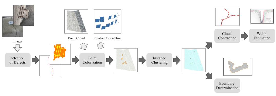
Figure 1 schematically depicts the components of the proposed workflow to transform the 2D information into 3D anomaly instances. It is assumed, that 3D reconstruction as described in Section 3.1 was successfully performed beforehand. The three major stages are the (1) the detection stage (“Detection of Defects”), the (2) mapping stage (“Point Colorization”) and the (3) extraction stage (“Instance Clustering”, “Cloud Contraction”, “Boundary Determination”, and “Width Estimation”). In the detection stage, a model for semantic segmentation is run on all images, returning class probabilities for all pixels of the input image. The mapping stage transfers these 2D class probabilities to the dense cloud yielding a semantically segmented point cloud. In the final extraction stage, the segmented point cloud is clustered and the respective subclouds are transformed into anomaly instances. For crack instances the crack width is subsequently estimated.
5 Detection Stage
For the detection on image level, off-the-shelf models for anomaly segmentation can be applied. The color images obtained e.g., by means of UAS, mobile phones, or hand cameras are processed by a segmentation model, which returns probability maps (also referred to as heatmaps) for each of the classes under investigation (crack, spalling, corrosion, and background). In this work, the three SOTA approaches TopoCrack pantoja2022topo , nnU-Net isensee2021nnu , and DetectionHMA benz2022image are used and compared. All of which are based on convolutional neural networks (CNN), a specific kind of artificial neural networks.
TopoCrack
With the goal of preserving the crack continuity, pantoja2022topo introduce a novel topological loss called TOPO loss and benchmark it against other losses. The base architecture is formed by TernausNet iglovikov2018ternausnet , which is a U-Net-based architecture with VGG11 encoder. Beside the dice loss, MSE for distance regression and TOPO loss for topology preservation are explored. Distance regression is based on truncated distance maps which are inferred from the segmentation labels. Each pixel in the distance map represents the distance to the closest crack. Distances over 20 pixels are truncated. The truncated distance maps are used with MSE loss to enforce the model to learn the correct distances to the closest crack. Based on oner2021promoting TOPO loss uses the concept of a maximin path. The maximin path is the path of minimal length connecting two pixels with the maximum values gathered along the way. In this context, the values are drawn from the distance map. For a continuous crack, the maximin paths that connect the background regions left and right of the crack contain a zero value, which is the crossing of the crack center. Maximin paths with values larger than zero indicate a discontinuity in the crack and are, thus, penalized. The combination of MSE and TOPO loss is reported to have an F score of 69% on the alongside published dataset.
nnU-Net
The nnU-Net approach was proposed by isensee2021nnu and published in Nature Methods in 2021. Ranking first in the majority of MICCAI888MICCAI stands for Medical Image Computing and Computer Assisted Interventions and refers to the highest-ranked annual computer science conference in the domain of medical imaging (ranking according to https://research.com/conference-rankings/computer-science, accessed on August 31, 2023). The conference is hosted by the MICCAI society http://www.miccai.org/. challenges in 2020 and 2021, nnU-Net attracted major attention in the field of medical imaging. An extended version of nnU-Net also won the AMOS challenge on abdominal multi-organ segmentation in 2022 isensee2023extending . The main benefits of nnU-Net are the minimum of manual intervention required for designing a model and the applicability on 2D and 3D segmentation tasks alike. benz2023ai indicate the usefulness of nnU-Net beyond the medical domain for 2D semantic segmentation of structural defects.
The term nnU-Net refers to ‘no new net’ since it does not propose any new network architecture, loss function, or training scheme isensee2021nnu . It rather systemizes the process of ‘methods configuration’ and delegates it to a set of fixed, rule-based, and empirical parameters for automated self-configuration. Based on the data fingerprint inferred from the particular dataset, heuristic rules guide the rule-based parameters of data handling (such as resampling strategies, intensity normalization, patch and batch sizes) and the adjustment of the architecture template. The training is based on fixed parameters with respect to the optimizer, learning rate, data augmentation, and loss function and runs in a scheme of 5-fold cross validation. In 5-fold cross-validation for each fold 20% of the training set is left out for validation purposes. 5-fold cross-validation eventually yields five models of the same architecture but different parameters. In a post-processing step an ensemble is empirically determined which combines the results of the five models. The architecture template of nnU-Net is based on the widely used U-Net design principle ronneberger2015u . nnU-Net was trained on the S2DS dataset (see below).
DetectionHMA
DetectionHMA999https://github.com/ben-z-original/detectionhma, accessed Dec 29, 2023. is proposed by benz2022image for detecting structural defects on concrete surfaces. It is based on hierarchical multi-scale attention approach by tao2020hierarchical , by the time a top performer with available code on the cityscapes benchmark cordts2016cityscapes . To overcome scale-invariance regularly observed for CNNS, HMA incorporate multiple scales and proposes a dynamic combination of results from different scales based on simultaneously generated attention maps. The attention maps are contrastively learned based on two scales only. For inference, however, the number of scales can be arbitrarily chosen. For DetectionHMA the scales 1.0, 0.5, and 0.25 rendered useful. As a backbone, HMA uses the HRNet-OCR yuan2020object , where OCR refers to object-contextual representations. The object-contextual representations are used to augment the pixel’s representation with contextual information. HMA uses the region mutual information (RMI) loss introduced by zhao2019region , which combines a cross-entropy component with a component representing mutual information.
DetectionHMA was trained on the S2DS (structural defect dataset) dataset, consisting of 743 images benz2022image . The dataset contains images from real inspection sites taken by various camera types and features the classes background, crack, spalling, corrosion, efflorescence, vegetation, and control point. Due to lack of 3D data for other classes, this works is confined to crack, spalling, corrosion, and background.
6 Mapping Stage
In the mapping stage, the results on image level are mapped into 3D space. More specifically, the probability information given in the 2D heatmaps are transferred onto the 3D point cloud. For that purpose, point colorization is performed with class labels acting as the respective colors. The points are projected into all views and the gathered information are aggregated into a single class label for each 3D point. This procedure is performed in parallel on batches of points of the point cloud.
The information aggregation from the views follows a fusion logic. It is assumed, that views more perpendicular to a point are supposed to contribute a higher degree to a point’s class than views from oblique directions. The deviation between view and point is measured by the angular difference between the point’s normal and the viewing direction. The information is aggregated by the following weighting scheme:
| (1) |
The term refers to the weight for view for a certain point of the dense point cloud. denotes the number of views the point is visible in. The view is only considered in case the angular deviation between the viewing direction and the point normal is in the range . The weighting is performed on each class channel individually. Subsequently, a class label is assigned to the point based on a winner-takes-all logic, i.e. the class with the highest value is assigned and the others are discarded.
7 Extraction Stage
The result of the mapping state is a point cloud, in which each point was assigned a certain class label. The classes considered in this work are crack, spalling, corrosion, and background. A point cloud is a set of independent points which per se do not have further knowledge about their neighborhood. Thus, it is unclear, if points of the same class do actually represent the same or different instances of a defect. For advanced quantitative analyses it is, however, essential to extract discrete instances of anomalies.
7.1 Clustering
It is assumed, that points of equal class and sufficient proximity represent the same instance of a defect. This assumption holds for crack, spalling, and corrosion alike. The density-based spatial clustering of applications with noise (DBSCAN) ester1996density algorithm groups points based on their distance. A specified minimal number of points within a certain distance forms a local high-density neighborhood which represents a cluster. Low-density neighborhoods are considered noise and consequently discarded.
The point cloud is split into three subclouds, one containing all crack points, one containing all spalling points, and one containing all corrosion points. All background points are discarded. DBSCAN runs on all subclouds and assigns a cluster ID to each point. Consequently, each point has information about which instance of a defect it represents. Due to their line-like character, cracks undergo different further processing than spalling and corrosion.
7.2 Cracks
The point cloud representation is not suited for quantitative analyses of the detected cracks such as determining the length, number of branches, or the direction of propagation. For that purpose, the clustered point cloud is transformed into a polyline representation referred to as (curve) skeleton or medial axis. Despite slight differences, the terms (curve) skeleton and medial axis are used interchangeably in this work. Figures 1(a) to 1(d) illustrate the stages of crack extraction.
Figure 1(a) shows the crack on a mesh with high-quality texture. By means of clustering, a subcloud is obtained which represents the specific instance of the crack, Figure 1(b). For extracting the medial axis of the subcloud, Laplacian-based contraction cao2010point is applied. Laplacian-based contraction minimizes the quadratic energy cao2010point :
| (2) |
represents the original point cloud, the contracted point cloud, is the Laplacian matrix, the contraction weight matrix, and the attraction weight matrix. The first term represents the geometric details, which is subject to smoothing. The second term preserves the geometric shape of the point cloud. The contraction and the attraction weights balance the tendency to collapse into one point (“contraction”) and to remain at the current location (“attraction”). Equation 2 is solved in iterative fashion with increasing contraction weights and updated attraction weights which maintain shape and avoid full collapse.
The contracted point cloud lacks information about the connectivity of points. Thus, a minimum spanning tree is computed yielding a connected graph with all points under minimal edge lengths. The nodes of the spanning tree have degree of 1, 2, or more. Nodes of degree 1 are end nodes, nodes of degree 2 are intermediate nodes, and nodes of degree 3 or more are furcation nodes. The spanning tree is recursively partitioned at every furcation node to obtain unbranched polylines. Figure 1(c) displays the extracted medial axis (red) for the respective point cloud. The detected crack consists of 5 unbranched polylines. Figure 1(d) shows the medial axis overlayed on the textured mesh in 3D space.
7.3 Crack Width Estimation
Once the 3D crack skeleton is extracted, the crack width can be estimated at individual points of the skeleton. For that purpose, the skeleton is sampled at regular intervals (e.g., 1 cm) and the given point is projected in all views. The single best view is selected according to a heuristic, which measures the angle between the viewing direction and point normal. From the given view, the intensity profile perpendicular to the propagation direction of the crack is extracted. The crack width can then be estimated by rectangle transform benz2021model : The approximately parabolic valley of the intensity profile is transformed into a rectangle of equal area yielding the estimated crack width. The chosen procedure is more robust towards image blur than other parabola-based methods.

7.3.1 Areal Defects
For areal defects such as spalling or corrosion skeletonization appears unsuited. Bounding boxes and convex hulls rather coarsely outline the extension of an anomaly on the structure’s surface. Thus, to approximate the area covered by the anomaly, a bounding polygon is computed. For that purpose, the subcloud representing the instance of a spalling or corrosion is mapped into 2D space. This is accomplished by performing principal component analysis (PCA) on the subcloud and retaining only the two dimensions with most explanatory power of variance. These dimensions are supposed to represent the plane, in which the defect is located. Note that the procedure might fail for defects at corners, wall projections, and other non-planar conditions.
The polygon extraction in 2D space is performed by means of alpha shapes edelsbrunner1983shape ; edelsbrunner1994three . Alpha shapes form a generalization of convex hulls and represent a bounding alpha hull, which encapsulates all respective points. The parameter represents the radius of a generalized disk and controls for the allowed concavity of the hull. For values close to zero the alpha-hull approximates the common convex hull. For the alpha hull is defined as “the intersection of all closed complements of discs” edelsbrunner1983shape with radius . With approaching negative infinity the bounding hull with highest concavity is returned, which corresponds to the minimum spanning tree of the points.
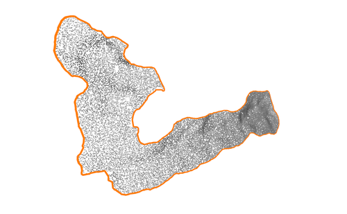
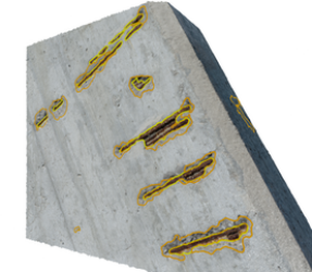
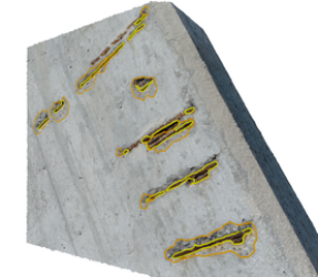
This work uses the implementation of alpha complexes101010https://github.com/bellockk/alphashape closely related to alpha shapes. Rather than arcs, alpha complexes compute an alpha hull consisting of straight lines derived from Delaunay triangulation. The choice of depends on the density of the points and the scale of the space. In this work the PCA transformed points are in normalized space and an alpha value of rendered suitable. Figures 2(a) to 2(e) illustrate the bounding polygon for an exposed reinforcement bar. Figure 2(a) show the textured mesh of an exposed rebar, which in this work is modeled as the union of co-occurring spalling and corrosion. Figure 2(b) is a depiction of the segmented point cloud derived by the procedure described in Section 6. Orange refers to spalling and yellow to corrosion. Figure 2(c) displays the bounding polygon computed with alpha complexes in the 2D space. For that purpose, the 3D subcloud was mapped to 2D space by means of PCA. The vertices of the polygon in 2D space directly correspond to vertices in the 3D from which the 3D bounding polygon can be inferred, Figure 2(d). Finally, the bounding 3D polygon can be displayed alongside the textured mesh, Figure 2(e).
8 Results
After introducing the metrics for quantitative evaluation, this section presents quantitative and qualitative results of the proposed workflow.
8.1 Evaluation Metrics
| Tol. | IoU % | AP % | ||||||||||||||||
| cm | Crack | Spall. | Corr. | Crack | Spall. | Corr. | ||||||||||||
|
|
|
||||||||||||||||
& – – – – – – – – – – 5.6 9.1 14.9 17.4 22.2 – – – – – – – – – – nnU-Net 1.0 2.0 4.0 6.0 8.0 66.0 71.3 78.9 85.0 90.6 10.8 17.4 27.6 43.7 55.3 35.1 75.8 96.9 99.5 100.0 8.6 10.4 17.5 31.8 44.8 3.2 16.2 47.6 61.7 72.0 36.8 68.8 73.3 78.6 78.6 DetectionHMA 1.0 2.0 4.0 6.0 8.0 89.0 91.5 94.9 96.7 99.0 15.8 25.4 40.5 58.3 77.2 17.0 47.0 81.5 89.7 95.8 22.3 27.8 45.0 52.6 62.5 16.0 32.7 44.5 53.3 64.0 11.6 49.0 55.6 55.6 64.1
| nnU-Net | nnU-Net (zoomed) | DetectionHMA | DetectionHMA (zoomed) |
 |
|
 |
|
 |
|
 |
|
The basic evaluation procedure for the quantitative evaluation corresponds to knapitsch2017tanks ; wang2018pixel2mesh ; gkioxari2019mesh . The vertices of both the medial axes and the bounding polygon are granted a positional tolerance based on the Euclidean distance measure . The true positives (TP), the false negatives (FN), and the false positives (FP) are defined as:
where denotes the true 3D vertices and the predicted 3D vertices of the medial axis resp. the bounding polygon. The square brackets refer to the Iverson brackets, which evaluate to one when the respective conditional is fulfilled, zero otherwise. The intersection-over-union is calculated by .
In order to assess the instance detection capabilities of the proposed workflow, the standard metric average precision is used, which derives from the integral of the precision-recall curve. An overlap threshold of of 50% is used; instances with more overlap are considered true positives, otherwise they form false positives or false negatives respectively. Analogously to IoU, is granted a positional tolerance represented by parameter .