Training embedding quantum kernels with data re-uploading quantum neural networks

Abstract

Kernel methods play a crucial role in machine learning and the Embedding Quantum Kernels (EQKs), an extension to quantum systems, have shown very promising performance. However, choosing the right embedding for EQKs is challenging. We address this by proposing a $p$-qubit Quantum Neural Network (QNN) based on data re-uploading to identify the optimal $q$-qubit EQK for a task ($p$-to-$q$). This method requires constructing the kernel matrix only once, offering improved efficiency. In particular, we focus on two cases: $n$-to-$n$, where we propose a scalable approach to train an $n$-qubit QNN, and $1$-to-$n$, demonstrating that the training of a single-qubit QNN can be leveraged to construct powerful EQKs.

I Introduction

Quantum computing is a promising computational paradigm for tackling some complex computational problems which are classically intractable. In particular, its potential in enhancing machine learning tasks has garnered significant attention Biamonte et al. (2017); Carleo et al. (2019); Dunjko and Briegel (2018); Dalzell et al. (2023) with parametrized quantum circuits as the most common approach Benedetti et al. (2019); Skolik et al. (2022); Schuld et al. (2020); Farhi and Neven (2018). Although there are evidences of quantum advantage in some tailored problems Sweke et al. (2021); Jerbi et al. (2021); Pirnay et al. (2023); Gyurik and Dunjko (2023), advantage over classical counterparts for practical applications remains as an area of active research.

Amidst the exploration of quantum machine learning models, previous studies, particularly in Refs. Havlíček et al. (2019); Schuld and Killoran (2019), have delineated a categorization into explicit and implicit models. In explicit models, data undergoes encoding into a quantum state, and then a parametrized measurement is performed. In contrast, implicit or kernel models are based on a weighted summation of inner products between encoded data points. A specialized category within parametrized quantum circuits, which can be considered separately, consists of data re-uploading models Pérez-Salinas et al. (2020). This architecture features an alternation between encoding and processing unitaries, yielding expressive models that have found extensive use Schuld et al. (2021a); Caro et al. (2021); Ono et al. (2023). However, Ref. Jerbi et al. (2023) shows that these models can be mapped onto an explicit model, thereby unifying these three approaches within the framework of linear models within Hilbert space.

Beyond this overarching theoretical framework, significant effort has been devoted to studying the performance of quantum kernel methods Huang et al. (2021); Peters et al. (2021); Bartkiewicz et al. (2020); Kusumoto et al. (2021). Furthermore, theorizing about them as a way to explain quantum machine learning models has also been pursued Schuld and Killoran (2019); Schuld (2021); Schuld et al. (2021b). This interest is substantiated by several compelling factors. Firstly, the act of embedding data into quantum states provides direct access to the exponentially vast quantum Hilbert space, where inner products can be efficiently computed. Secondly, the creation of embedding quantum kernels that pose classical intractability yet offers the potential for quantum advantages Liu et al. (2021). Finally, in both classical machine learning and kernel methods, the representer theorem Schölkopf and Smola (2001) ensures that they consistently achieve a training loss lower than or equal to that of explicit models, provided the same encoding and training set are considered. However, it is worth noting that this enhanced expressivity may be accompanied by reduced generalization capability, a point explored and discussed in Ref. Jerbi et al. (2023).

While the arguments above might suggest a preference for kernel or implicit models over explicit ones, practical challenges persist. Firstly, the computational complexity associated with constructing the kernel matrix scales quadratically with the number of training samples. Additionally, selecting the appropriate embedding that defines the kernel function is contingent on the specific problem at hand, demanding careful consideration. Regarding the last one, two approaches to train kernels customized for the dataset in question have been considered: multiple kernel learning and kernel target alignment. In the former, a combination of kernel functions is trained to minimize an empirical risk function Vedaie et al. (2020); Ghukasyan et al. (2023). In the latter, it is defined a kernel using an embedding ansatz which is trained to align with an ideal kernel Hubregtsen et al. (2022). However, these techniques require the computation of the kernel matrix at each training iteration, incurring substantial computational costs.

In this Article, we employ a quantum neural network (QNN) to create an embedding quantum kernel (EQK). This strategy utilizes QNN training to construct the corresponding kernel matrix, significantly reducing the computational cost when compared to constructing the kernel matrix at each training step. In particular, we utilize the data re-uploading architecture for the QNN and propose a method to straightforwardly scale the training up to an $p-$qubit QNN. Following training on a given dataset, this QNN is used to generate a $q-$qubit EQK. This construction is denoted as the $p$-to-$q$ approach. Here, we will focus on two specific cases: the $n$-to-$n$ and the $1$-to-$n$. The former is fundamentally relevant, since we can prove that the classification accuracy of the QNN never decreases with $n$ and that entanglement plays a role in this accuracy. Additionally, we have empirically observed that the classification accuracy of the EQK not only is higher than the one of the QNN, as expected, but also that it does not decrease with $n$. We also propose the use of the training of a single-qubit QNN to create an $n$-qubit EQK with entanglement, referred to as the $1$-to-$n$ approach. We substantiate our proposals with numerical evidence, demonstrating that the training of a small-sized QNN, potentially even simulatable classically, adeptly selects parameters to form a potent EQK tailored for a specific task. Our results consider up to 10 qubits, showing that our approach circumvents typical training challenges associated with scaling parametrized quantum circuits.

The article is organized into the following sections. We begin by introducing quantum kernel methods and EQKs. Afterwards, we present the data re-uploading architecture and our approach to scaling it up to an $n$-qubit QNN. Subsequently, we detail the construction of EQKs derived from the training of these QNNs. Finally, we present numerical results supporting the practicability of our approach.

II Quantum kernel methods

Quantum machine learning models can be categorized into explicit and implicit models, as discussed in Refs. Schuld and Killoran (2019); Havlíček et al. (2019). Explicit models are based on parametrized quantum circuits Benedetti et al. (2019); Abbas et al. (2021); Cerezo et al. (2021); Bharti et al. (2022), which are tailored to process classical information $𝒙$ encoded into a quantum state as $\rho (𝒙)=S(𝒙)|0⟩{⟨0|}^{\otimes n}{S}^{†}(𝒙)$, where $S$ refers to some quantum embedding. These models have proven resilient to noise Sharma et al. (2020), making them attractive for seeking quantum advantages in near-term quantum processors. However, they face scalability challenges due to the barren plateau problem during training McClean et al. (2018); Cerezo et al. (2021); Holmes et al. (2022); Anschuetz and Kiani (2022); Ragone et al. (2023). Implicit or kernel models, on the other hand, are defined by the linear combination

$$f_{𝜶,X}=\sum _{i=1}^M{\alpha }_{i}k(𝒙,{𝒙}_i),$$ (1)

where $k(𝒙,{𝒙}_i)=\mathrm{tr}(\rho (𝒙)\rho ({𝒙}_i))$ is the kernel function and ${\{{𝒙}_i\}}_{i=1}^M$ denotes training points from a training set $X$. An important insight from classical machine learning theory is captured by the representer theorem. This theorem asserts that, when provided with a feature encoding and a training set, implicit models in the form of Eq. 1 consistently attain training losses that are either equal to or lower than those of explicit quantum models.

Determining the optimal $𝜶$ parameters for implicit models involves solving a convex optimization problem, necessitating the construction of the kernel matrix $K$ with entries $k_{ij}=k({𝒙}_i,{𝒙}_j)$. To accomplish this, inner products between all training points must be evaluated on a quantum computer Buhrman et al. (2001); Fanizza et al. (2020); Cincio et al. (2018), involving $𝒪(M^2)$ evaluations. Although there are instances where these inner products can be computed without explicitly constructing the feature map, our primary focus here is on embedding quantum kernels (EQKs). EQKs, prevalent in quantum kernel literature and proven to be universal in Ref. Gil-Fuster et al. (2023), are constructed as follows:

$$k({𝒙}_i,{𝒙}_j)={|⟨\varphi ({𝒙}_i)|\varphi ({𝒙}_j)⟩|}^2={|⟨\mathrm{𝟎}|S^{†}({𝒙}_i)S({𝒙}_j)|\mathrm{𝟎}⟩|}^2,$$ (2)

where $|\mathrm{𝟎}⟩:={|0⟩}^{\otimes n}$. These overlap evaluations serve as input for a support vector machine (SVM) algorithm. Although quantum SVM approaches have been explored Rebentrost et al. (2014); Park et al. (2023), we assume classical computation for this step in this work, incurring a time complexity of $𝒪(M^3)$.

Given the representer theorem and the inherent capability of quantum devices to access exponentially large feature spaces, quantum kernel methods emerge as promising candidates for optimal quantum machine learning models Schuld (2021). However, they come with their challenges, such as the exponentially vanishing of kernel values Thanasilp et al. (2022); Kübler et al. (2021), and, as addressed in this work, the critical issue of selecting the appropriate kernel for a specific task.

To identify the optimal kernel, the common strategy involves employing a parametrized quantum embedding $S_{𝜽}(𝒙)$ Lloyd et al. (2020), where $𝜽$ represents the trainable parameters. This embedding defines a trainable quantum kernel $k_{𝜽}(𝒙)$, which is then optimized based on a specific figure of merit. In the study by Hubregtsen et al. Hubregtsen et al. (2022), the optimization problem is formulated using kernel target alignment. Another avenue explored in works such as Vedaie et al. (2020); Ghukasyan et al. (2023) involves multiple kernel learning, where the goal is to determine the optimal combination of different kernels for a specific task. However, these approaches require constructing the kernel matrix at each training step, which implies a high computational cost. In our work, we propose a novel method for training embedding quantum kernels that only necessitates constructing the kernel matrix once.

Figure 1: Iterative training of a two-qubit data re-uploading QNN. In Step 1, a single-qubit QNN is trained to obtain optimal model parameters denoted as ${𝜽}^{\ast }$. Moving to Step 2, training for the two-qubit QNN is initiated, initializing new extra parameters to 0, while the parameters of the first qubit are set to ${𝜽}^{\ast }$. This iterative approach can scale the QNN up to $n\le L+1$ qubits, ensuring that the $n$-qubit QNN performs at least as effectively as the $n-1$ version.

III Scaling data re-uploading for $n-$qubit QNN

Figure 2: An schematic illustration of how a single-qubit EQK, constructed from a single-qubit QNN, can enhance classification outcomes. The QNN aims to group points of the same class while fixing the decision plane (left Bloch sphere). The SVM, employing the single-qubit EQK, fine-tunes the decision boundary parameters to find the optimal hyperplane (right Bloch sphere). As a result, data points that were previously misclassified can now be correctly assigned to their respective labels. We also provide an example demonstrating a scenario in which the QNN accuracy plateaus out for a specific dataset. By using the corresponding EQK, we obtain however an increase in accuracy, denoted as $\mathrm{\Delta }\mathrm{Acc}$.

As reported by Pérez-Salinas et al. in Ref. Pérez-Salinas et al. (2020), the data re-uploading model incorporates layers composed of data-encoding and training unitaries. This approach effectively introduces non-linearities to the model allowing to capture complex patterns on data Schuld et al. (2021a); Casas and Cervera-Lierta (2023); Caro et al. (2021); Barthe and Pérez-Salinas (2023). In fact, it has been demonstrated that a single qubit quantum classifier possesses universal capabilities Pérez-Salinas et al. (2021).

While various encoding strategies could be considered for this architecture, we specifically adopt the easiest one defining

$${\mathrm{QNN}}_{𝜽}(𝒙)\equiv \prod _{l=1}^{L}U({𝜽}_l)U(𝒙)=U({𝜽}_L)U(𝒙)\mathrm{\dots }U({𝜽}_1)U(𝒙).$$ (3)

Here, $L$ denotes the number of layers, $U$ represents a generic $\mathrm{SU}(2)$ unitary, and the vector $𝜽=\{{𝜽}_1,\mathrm{\dots },{𝜽}_L\}$ encompasses the trainable parameters. To leverage this model to construct a binary classifier, one must select two label states that are maximally separated in Hilbert space. The training objective involves instructing the model to collectively rotate points belonging to the same class, bringing them closer to their corresponding label state.

Starting with the data re-uploading single-qubit QNN architecture, we can naturally extend it to create multi-qubit QNNs. The introduction of more qubits enhances the model’s expressivity by increasing the number of trainable parameters per layer and offering the potential for entanglement between qubits which enhances the expressivity of the model Panadero et al. (2023).

In this work, we propose an iterative training approach for multi-qubit QNNs. In our construction, the $n$-qubit QNN is defined as

$${\mathrm{QNN}}_{𝜽,𝝋}(𝒙)=\prod _{l=1}^L\left(\prod _{s=1}^{n-1}{\mathrm{CU}}_{s+1}^s({𝝋}_l^{(s)})\left(\underset{r=1}{\overset{n}{⨂}}U({𝜽}_l^{(r)})\right)U{(𝒙)}^{\otimes n}\right),$$ (4)

where ${\mathrm{CU}}_{s+1}^s$ denotes the controlled version of the general $\mathrm{SU}(2)$ unitary with control in the $(s+1)$-th qubit and target in the $s$-th qubit, and $𝜽$ and $𝝋$ refer to the trainable parameters of single-qubit and two-qubit gates, respectively. The total number of trainable parameters in this architecture is $3(2n-1)L$.

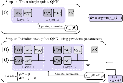
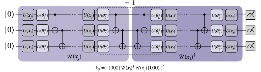
For the training of the $n$-qubit QNN, we propose an iterative construction starting from a single-qubit QNN. The initialization process is depicted in Figure 1. Initially, we train a single-qubit QNN and utilize its parameters to initialize the two-qubit QNN. During the initialization of the two-qubit QNN, we set ${𝝋}_l^{(1)}=\mathrm{𝟎}$ for all $l\in [1,L]$, initializing the parameters of the first qubit with those obtained from the training of the single-qubit step. Consequently, the entangling layers do not have any action, ensuring that, with a local measurement on the first qubit, we commence in the output state of the single-qubit QNN training.

This process can be employed to scale up the QNN architecture, allowing the construction of QNNs with up to $n=L+1$ qubits. When adding an extra qubit, the supplementary entangling gates are initialized as identities, and the training begins with the optimal parameters obtained from the previous step. Essentially, this formalized approach signifies a systematic and scalable improvement in the QNN’s performance with the incorporation of each additional qubit.

Figure 3: Embedding quantum kernels generated from quantum neural networks training. The kernel matrix element $k_{ij}$ is defined as the probability of measuring all qubits in the state $|0⟩$, denoted as $P_{\mathrm{𝟎}}$. On the left, we have the $n$-to-$n$ proposal, constructed by directly utilizing the trained data re-uploading $n$-qubit QNN as a quantum feature map. On the right, we show the construction of an Embedded EQK from the training of a single-qubit QNN, named as $1$-to-$n$.

IV Constructing EQKs from QNN training

In this section, we propose a method for constructing trained embedding quantum kernels (EQK) using data re-uploading quantum neural networks (QNN). The idea is to train the QNN for a classification task and leverage its architecture to generate EQKs tailored to the specific task, thereby enhancing performance on the given dataset. The motivation for combining these two binary classification approaches, QNN and kernel methods, arises from two perspectives.

Firstly, we investigate whether the QNN can effectively select a suitable embedding kernel for a specific task. This approach may lead to more efficient kernel training compared to previous methods, as we only need to construct the kernel matrix once. Secondly, the QNN’s performance is contingent on its training. Utilizing the corresponding EQK construction might produce superior results compared to relying solely on the QNN, even in cases where the training process has not been optimal. Numerical results illustrating this can be found in Appendix E.

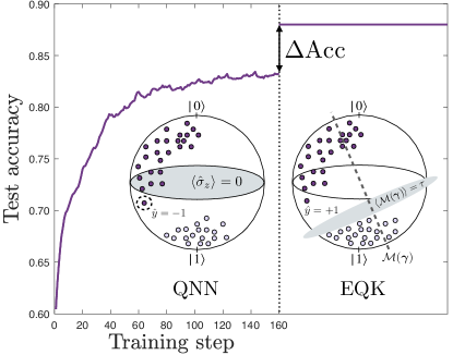
The underlying concept of this method is formalized in the Appendix and clarified in Figure 2, specifically for a single-qubit scenario. Initially, the QNN rotates data points of the same class near their label state while maintaining the decision hyperplane fixed. This hyperplane is taken as the equator of the Bloch sphere, i.e., $⟨{\widehat{\sigma }}_z⟩=0$. After training the QNN, the resulting feature map is obtained by preserving the parameters acquired during training. This feature map is then utilized to construct an EQK. The subsequent application of the SVM algorithm, using this kernel, aims to identify the optimal separation hyperplane in the feature space. In this context, the optimization is equivalent to adjusting the optimal measurement $ℳ(𝜸)$ while keeping the data points fixed.

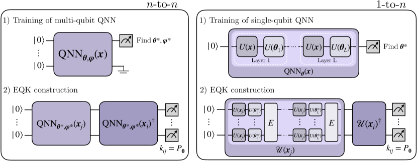
Building upon this insight, we propose constructing EQKs using QNN training in two ways: the $n$-to-$n$ approach and the $1$-to-$n$. In the first one, an $n$-qubit QNN is trained using the iterative method proposed earlier to directly construct the corresponding EQK of $n$ qubits. As depicted in Figure 3, a multi-qubit QNN of the form of Eq. 4 is trained while fixing the trainable parameters of the embedding ${𝜽}^{\ast }$ and ${𝝋}^{\ast }$. Then, these parameters are subsequently used to construct an EQK which is defined by

$$k_{ij}={|⟨\mathrm{𝟎}|{\mathrm{QNN}}_{{𝜽}^{\ast },{𝝋}^{\ast }}{({𝒙}_i)}^{†}{\mathrm{QNN}}_{{𝜽}^{\ast },{𝝋}^{\ast }}({𝒙}_j)|\mathrm{𝟎}⟩|}^2.$$ (5)

This method allows us to scale the QNN as much as possible during training, and when it reaches a performance plateau, we can utilize the trained feature map to construct an EQK.

In the $1$-to-$n$ construction, we train a single-qubit ${\mathrm{QNN}}_{𝜽}$ from Eq. 3, fixing the ${𝜽}^{\ast }$ and we leverage this training to construct the kernel

(6)

where $E$ denotes an entangling operation, such as a cascade of $\mathrm{CNOT}$ or $\mathrm{CZ}$ gates, among other possibilities. It is worth noting that the training is conducted for a single-qubit QNN and does not explicitly consider entanglement. Nevertheless, we will present numerical results demonstrating that this training alone is sufficient to select parameters for constructing a customized multi-qubit kernel tailored to a specific task.

Certainly, one can combine both the $n$-to-$n$ and the $1$-to-$n$ architectures and generalize it to $n$-to-$m\cdot n$, where $m$ represents some integer. In this scenario, an $n$-qubit QNN is trained and utilized to implement the same design as in the $1$-to-$n$ construction. However, in this case, each qubit of the QNN is embedded into $m$ qubits, introducing entanglement between layers.

V Numerical results

Let us now explore the practical implementation of our approaches and evaluate their performance across various datasets detailed in Appendix F. Both the training and test sets consist of 500 data points each.

For the QNN training in this section, we employ the Adam optimizer with a batch size of 24. In the initial step for the QNN training ($n=1$), we use a learning rate of 0.05 and consider 30 epochs. For $n>1$, we use a learning rate of 0.005 and 10 epochs.

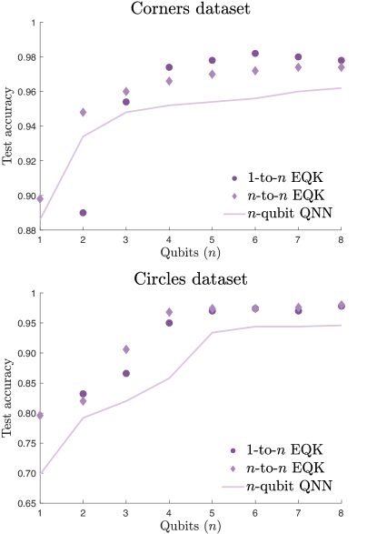
The results presented in Figure 4 demonstrate the test accuracies for two distinct datasets—the corners dataset and the circles dataset—for the $1$-to-$n$ and the $n$-to-$n$ constructions as functions of the number of qubits $n$. These experiments consider $L=7$ layers, scaling up the QNN to $n=L+1=8$. In the $1$-to-$n$ construction, we introduce entanglement between layers using a cascade of CNOT gates, defined as

$$E=\prod _{s=1}^{n-1}{\mathrm{CNOT}}_s^{s+1},$$ (7)

where the subscript refers to the control qubit, and the superscript refers to the target qubit.

The numerical experiments illustrate a consistent improvement in the performance of the $n$-qubit QNN as more qubits are introduced for both datasets. Additionally, the corresponding kernel, represented by the $n$-to-$n$ construction, exhibits enhanced performance compared to the QNN alone. Interestingly, the $1$-to-$n$ construction performs remarkably well, showing a rapid increase in performance with a small number of qubits, although it eventually plateaus. While the improvement in the $n$-to-$n$ scenario is slower, its performance consistently surpasses that of the QNN, and the scaling of this model is consistent and rigorous. For additional numerical experiments, refer to Appendix G.

These results demonstrate, on one hand, the scalability of a data re-uploading QNN and the improved performance achieved by constructing the corresponding EQK. On the other hand, they highlight the capability to create complex kernels through the training of simple QNN architectures. Despite the small QNNs being trainable using a classical computer, the obtained parameters could be utilized to construct a classically hard embedding quantum kernel.

Figure 4: Test accuracies for the two EQK architectures presented in this work, namely $1$-to-$n$ and $n$-to-$n$, plotted against the number of qubits $n$. Additionally, we include the test accuracy of the $n$-qubit QNN using the iterative training proposed. Results are showcased for the corners dataset in the top plot and the circles dataset in the bottom plot.

VI Conclusions

We have addressed the challenge of training a $q$-qubit embedding quantum kernel by introducing a practical approach that constructs them from a data re-uploading $p$-qubit quantum neural network. This method significantly reduces computational costs compared to previous techniques in which the kernel matrix was constructed at each training step. We focus on two specific cases for constructing embedding quantum kernels, namely, the $n$-to-$n$ and the $1$-to-$n$ cases. The first involves using the output of the training of an $n$-qubit QNN directly as a feature map (referred to as the $n$-to-$n$ approach), for which we have proposed a scalable training method. The second approach enables the creation of multi-qubit EQKs with entanglement from the training of a single-qubit QNN (referred to as the $1$-to-$n$ approach). Given the current limitations in scaling parametrized quantum circuits, our combined approach offers an alternative for creating trainable scalable kernels as quantum machine learning models, mitigating the challenges associated with their scalability and reducing the dependence on the training for model success. Moreover, the $1$-to-$n$ approach can be considered a quantum inspired proposal, paving the way for exploring the construction of classically hard-to-estimate kernels from the training of small architectures, even those that can be simulated with a classical computer.

VII Acknowledgements

The authors would like to thank Maria Schuld for her valuable comments which led to a more solid presentation of the results and Sofiene Yerbi and Adrián Pérez-Salinas for their worthy insights during QTML 2023. PR and YB acknowledge financial support from the CDTI within the Misiones 2021 program and the Ministry of Science and Innovation under the Recovery, Transformation and Resilience Plan—Next Generation EU under the project “CUCO: Quantum Computing and its Application to Strategic Industries”. PR and MS acknowledge support from EU FET Open project EPIQUS (899368) and HORIZON-CL4- 2022-QUANTUM01-SGA project 101113946 OpenSuperQPlus100 of the EU Flagship on Quantum Technologies, the Spanish Ramón y Cajal Grant RYC-2020-030503-I, project Grant No. PID2021-125823NA-I00 funded by MCIN/AEI/10.13039/501100011033 and by “ERDF A way of making Europe” and “ERDF Invest in your Future”, and from the IKUR Strategy under the collaboration agreement between Ikerbasque Foundation and BCAM on behalf of the Department of Education of the Basque Government. This project has also received support from the Spanish Ministry of Economic Affairs and Digital Transformation through the QUANTUM ENIA project call - Quantum Spain, and by the EU through the Recovery, Transformation and Resilience Plan - NextGenerationEU. YB acknowledges support from the Spanish Government via the project PID2021-126694NA- C22 (MCIU/AEI/FEDER, EU).

Appendix A Related work on quantum kernel training

One of the main drawbacks of quantum kernel methods is determining the best kernel which depends on the specific problem. In cases where no prior knowledge about the input data is available, approaches have been developed to construct parametrized embedding quantum kernels that are trained for a specific task. These kernel training methods are based on multiple kernel learning Vedaie et al. (2020); Ghukasyan et al. (2023) and kernel target alignment Hubregtsen et al. (2022).

A.1 Multiple kernel learning

Multiple kernel learning methods involve the creation of a combined kernel

$$k_{𝝋,𝝎}({𝒙}_i,{𝒙}_j)=f_{𝝎}\left({\{k_{𝝋}^{(r)}({𝒙}_i,{𝒙}_j)\}}_{r=1}^R\right),$$ (8)

where $k_{𝝋}^{(r)}$ represents a set of parametrized embedding quantum kernels, and $f_{𝝎}$ is a combination function. Two common choices for this function result in either a linear kernel combination

$$k_{𝝋,𝝎}({𝒙}_i,{𝒙}_j)=\sum _{r=1}^R{\omega }_r{k}_{𝝋}^{(r)}({𝒙}_i,{𝒙}_j),$$ (9)

or a multiplicative kernel combination

$$k_{𝝋}({𝒙}_i,{𝒙}_j)=\prod _{r=1}^R{k}_{𝝋}^{(r)}({𝒙}_i,{𝒙}_j).$$ (10)

When it comes to choosing model parameters, in Ref. Vedaie et al. (2020) they use an empirical risk function to minimize, while in Ref. Ghukasyan et al. (2023) the authors opt for a convex minimization problem. However, in both constructions a complete kernel matrix is computed at each optimization step.

A.2 Kernel target alignment

Training kernels using kernel target alignment is based on the similarity measure between two kernel matrices, denoted as $K_A$ and $K_B$. This similarity measure, known as kernel alignment Holmes and Jain (2006), is defined as

$$KA(K_A,K_B)=\frac{\mathrm{tr}(K_A{K}_B)}{\sqrt{\mathrm{tr}(K_A^2)\cdot \mathrm{tr}(K_B^2)}}.$$ (11)

and corresponds to the cosine of the angle between kernel matrices if we see them as vectors in the space of matrices with the Hilbert-Schmidt inner product. The use of kernel alignment to train kernels is by defining the ideal kernel matrix $K^{\ast }$ whose entries are $k_{ij}^{\ast }=k^{\ast }({𝒙}_i,{𝒙}_j)=y_i{y}_j$. Given a parametrized quantum embedding kernel $k_{𝜽}({𝒙}_i,{𝒙}_j)={|⟨{\varphi }_{𝜽}({𝒙}_i)|{\varphi }_{𝜽}({𝒙}_j)⟩|}^2$ whose kernel matrix is named as $K_{𝜽}$, the kernel-target alignment is defined as the kernel alignment between $K$ and the ideal kernel, i.e.

$$TA(K_{𝜽})=KA(K_{𝜽},K^{\ast })=\frac{{\sum }_{ij}{y}_i{y}_j{k}_{𝜽}({𝒙}_i,{𝒙}_j)}{M\sqrt{{\sum }_{ij}{k}_{𝜽}{({𝒙}_i,{𝒙}_j)}^2}},$$ (12)

where we used that $y_i^2=1$ independently from the label and $M$ is the number of training points. Thus, authors in Ref. Hubregtsen et al. (2022) use this quantity as cost function which is minimized using gradient descent over the $𝜽$ parameters. This strategy is closely related to the approach outlined in Ref. Lloyd et al. (2020), where the authors explore the construction of quantum feature maps with the aim of maximizing the separation between different classes in Hilbert space. However, in the case of the kernel target alignment strategy, similar to multiple kernel learning, the construction of the kernel matrix (or at least a subset of it) at each training step is required.

Appendix B Data re-uploading

To construct a data re-uploading QNN for binary classification, each label is associated with a unique quantum state, aiming to maximize the separation in the Bloch sphere. For the single qubit quantum classifier, the labels +1 and -1 are represented by the computational basis states $|0⟩$ and $|1⟩$, respectively. The objective is to appropriately tune the parameters ${\{{𝜽}_l\}}_{l=1}^L$ that define the state

$$|{\varphi }_{𝜽}({𝒙}_i)⟩=U({𝜽}_L)U(𝒙)\mathrm{\dots }U({𝜽}_1)U(𝒙)|0⟩,$$ (13)

to rotate the data points of the same class close to their corresponding label state. To achieve this, we use the fidelity cost function

$$f_{\mathrm{cost}}=\frac{1}{M}\sum _{i=1}^M\left(1-{|⟨{\varphi }_l^i|{\varphi }_{𝜽}({𝒙}_i)⟩|}^2\right),$$ (14)

where $|{\varphi }_l^i⟩$ represents the correct label state for the data point ${𝒙}_i$. This optimization process occurs on a classical processor. Once the model is trained, the quantum circuit is applied to a test data point ${𝒙}_t$, and the probability of obtaining one of the label states is measured. If this probability surpasses a certain threshold (set as 1/2 in this case), the data point is classified into the corresponding label state class. Formally, the decision rule can be expressed as

(15)

When consider a multi-qubit architecture, the idea is the same but we need to properly choose the corresponding label states. In this work, for a $n$-qubit QNN we consider as label states the ones defined by the projectors $|0⟩⟨0|\otimes {\mathrm{𝟙}}^{(n-1)}$ and $|1⟩⟨1|\otimes {\mathrm{𝟙}}^{(n-1)}$, which corresponds to a local measurement in the first qubit.

Appendix C Connection with the representer theorem

In this section, we aim to leverage the representer theorem to demonstrate that the kernels derived from the data re-uploading Quantum Neural Network (QNN) will be at least as effective as the corresponding QNN. In our construction, the $n$-qubit QNN is defined in Eq. 4 in the main text. There, we can extract the last layer to separate it into a variational part, which will be absorbed into the measurement when we define the corresponding quantum model, and the encoding part which will define the quantum feature map for the construction of the kernel. This corresponds to

$${\mathrm{QNN}}_{𝜽,𝝋}(𝒙)=\underset{=V(𝝀,𝝎)}{\underbrace{\prod _{s=1}^{n-1}{\mathrm{CU}}_{s+1}^s({𝝀}^{(s)})\left(\underset{r=1}{\overset{n}{⨂}}U({𝝎}^{(r)})\right)}}\underset{=S_{𝜽,𝝋}(𝒙)}{\underbrace{\prod _{l=1}^{L-1}\left(\prod _{s=1}^{n-1}{\mathrm{CU}}_{s+1}^s({𝝋}_l^{(s)})\left(\underset{r=1}{\overset{n}{⨂}}U({𝜽}_l^{(r)})\right)U{(𝒙)}^{\otimes n}\right)}},$$ (16)

where we defined $𝝀\equiv {𝝋}_L$ and $𝝎\equiv {𝜽}_L$. This formulation aligns with the definition of a quantum model from Ref. Schuld (2021),

$$f(𝒙)=\mathrm{tr}(\rho (𝒙)ℳ).$$ (17)

In our case, $\rho (𝒙):={\rho }_{𝜽,𝝋}(𝒙)=S_{𝜽,𝝋}(𝒙)|0⟩{⟨0|}^{\otimes n}{S}_{𝜽,𝝋}{(𝒙)}^{†}$, and the variational measurement $ℳ:={ℳ}_{𝝀,𝝎}=V(𝝀,𝝎)({\widehat{\sigma }}_z\otimes {\mathrm{𝟙}}^{(n-1)})V{(𝝀,𝝎)}^{†}$.

Once this model is trained over a dataset, we determine the parameters that minimize the $f_{\mathrm{cost}}$ defined in the previous section, fixing ${𝜷}^{\ast },{𝜽}^{\ast },{𝝀}^{\ast }$, and ${𝝎}^{\ast }$. If we now use the corresponding feature map $S_{{𝜽}^{\ast },{𝝋}^{\ast }}$ to construct an embedding quantum kernel, we are effectively replacing the measurement from the optimization ${ℳ}_{{𝝀}^{\ast },{𝝎}^{\ast }}$ by the optimal measurement

$${ℳ}_{\mathrm{opt}}=\sum _{m=1}^M{\alpha }_m{\rho }_{{𝜽}^{\ast },{𝝋}^{\ast }}({𝒙}_m)$$ (18)

which, by the representer theorem, defines the optimal quantum model

$$f_{\mathrm{opt}}(𝒙)=\sum _{m=1}^M{\alpha }_m\mathrm{tr}\left({\rho }_{{𝜽}^{\ast },{𝝋}^{\ast }}(𝒙){\rho }_{{𝜽}^{\ast },{𝝋}^{\ast }}({𝒙}_m)\right)$$ (19)

that minimizes the regularized empirical risk function. Thus, we proved that constructing the embedding quantum kernel from QNN training will perform equally or better in terms of training loss than the QNN alone.

Appendix D Hyperplane defined in the Bloch sphere

The objective of the data re-uploading quantum neural network (QNN) is to map all points with label +1 to the $|0⟩$ state on the Bloch sphere, while mapping points with label -1 to the $|1⟩$ state. In an ideal scenario, all +1 points would be rotated to the $|0⟩$ state and all -1 points to the $|1⟩$ state. Using this feature map to construct the embedding quantum kernel, all points would be support vectors associated to the same Lagrange multiplier $\alpha$. The SVM generates a separating hyperplane defined by the equation

$$\sum _{i\in \mathrm{SV}}{\alpha }_i{y}_{i}k({𝒙}_i,𝒙)+b=0.$$ (20)

In this scenario, assuming a balanced dataset translates to an equal number of support vectors, denoted as $N_{\mathrm{SV}}$, for each class, and results in $b=0$ due to symmetry. Working with this equation by considering the sum of support vectors separately for the +1 class (${\mathrm{SV}}_{+1}$) and -1 class (${\mathrm{SV}}_{-1}$), we obtain

$$\begin{array}{c}\hfill \sum _{i\in {\mathrm{SV}}_{+1}}{\alpha }_i{y}_i|⟨\varphi ({𝒙}_i)|\varphi (𝒙)⟩{|}^2+\sum _{i\in {\mathrm{SV}}_{+1}}{\alpha }_i{y}_i|⟨\varphi ({𝒙}_i)|\varphi (𝒙)⟩{|}^2=N_{\mathrm{SV}}\alpha |⟨0|\varphi (𝒙⟩{|}^2-N_{\mathrm{SV}}\alpha |⟨1|\varphi (𝒙⟩{|}^2=0,\end{array}$$ (21)

which is equivalent to the hyperplane defined by

$$|⟨0|\varphi (𝒙⟩{|}^2=|⟨1|\varphi (𝒙⟩{|}^2,$$ (22)

mirroring the decision boundary of the QNN part. Therefore, in the case of a perfect training, the SVM becomes redundant. Even if the points are not perfectly mapped to their label states and the separating hyperplane of the SVM is not exactly the one from Eq. 22, as long as all points are correctly classified by the QNN, the SVM will yield the same results. Thus, the SVM part is only meaningful for the single-qubit QNN to construct a single-qubit EQK case when the QNN training is suboptimal and requires to adjust the measurement of the decision boundary.

Appendix E Noisy simulations

We have introduced a combined protocol for binary classification. It is worth noting that the kernel estimation part involves the utilization of a quantum circuit with twice the depth of the QNN part. In practical implementations on current noisy intermediate-scale quantum devices, the consideration of a larger circuit warrants careful attention. This is due to the susceptibility of larger circuits to elevated noise levels, potentially affecting the overall performance.

As previously mentioned, increasing the number of layers in the model enhances its expressivity. However, when constructing the kernel using a high number of layers, noise can have a detrimental impact on the performance, resulting in poorer results for the combined protocol compared to using only the QNN. Therefore, in this section, our objective is to perform simulations to visualize the trade-off between the number of layers in the QNN and using the combined protocol.

To characterize the noise incorporated into these simulations, we employ the operator sum representation of the noise channel $\epsilon$ acting on a quantum state $\rho$,

$$\epsilon (\rho )=\sum _k{E}_k\rho E_k^{†},$$ (23)

where $E_k$ represents the respective Kraus operators. In our simulations, we account for two single-qubit noise channels that are applied after each quantum gate. Firstly, we consider amplitude damping error which is described by the Kraus operators

$K_0$ (24)

$K_1$ (25)

Here, $\gamma \in [0,1]$ is the amplitude damping probability, which can be defined as $p=1-e^{-\mathrm{\Delta }t/T_1}$, with $T_1$ representing the thermal relaxation time and $\mathrm{\Delta }t$ denoting the duration of application of a quantum gate. The second noise source under consideration is the phase flip error, which can be described by the following Kraus operators

$K_0$ (26)

$K_1$ (27)

In this case, $\alpha \in [0,1]$ represents the probability of a phase flip error, which can be defined as $2\alpha =1-e^{-\mathrm{\Delta }t/(2T_2)}$, with $T_2$ denoting the spin-spin relaxation time or dephasing time. The value of $\alpha$ also falls within the interval $[0,1]$.

The current state-of-the-art experimental values for the noise parameters of a superconducting quantum processor are as follows: $T_1$ falls within the range of $50-150\mu s$, $T_2$ is in the range of $25-75\mu s$, and $\mathrm{\Delta }t$ varies from $10-50ns$. It is important to note that noise becomes more pronounced when $T_1$ and $T_2$ decrease and/or when $\mathrm{\Delta }t$ increases. To explore the scenario with the worst noise, we consider the extreme values within these ranges, leading to ${\gamma }^{\ast }=0.001$ and ${\alpha }^{\ast }=0.0005$.

In our simulations, we simplify the noise characterization by defining a noise strength parameter $\tau \equiv \alpha =\gamma$ for the sake of simplicity. We choose the single-qubit data re-uploading quantum neural network (QNN) as the kernel selection part. To observe a transition where it is no longer advantageous to include the support vector machine (SVM) part, we explore values of $\tau$ ranging from $0.005$ to $0.030$ in steps of $0.005$, while also including the noiseless case where $\tau =0$. These values correspond to examining the range $5{\gamma }^{\ast }\le \gamma \le 30{\gamma }^{\ast }$ and $10{\alpha }^{\ast }\le \alpha \le 60{\alpha }^{\ast }$. Notably, even in these highly adverse conditions, which are significantly worse than those of current real hardware quantum devices, we find that the combined protocol remains suitable. This conclusion aligns with expectations since the protocol utilizes only a small number of qubits and quantum gates.

Figure E.1: Relative improvement, as a function of the number of layers and noise strength, comparing the single qubit QNN accuracy performance with the combined protocol utilizing a two-qubit embedding kernel. Results are shown for the sinus, corners, and spiral datasets.

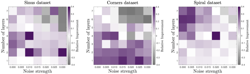
In Figure E.1, we present the relative improvement, denoted as

$$\text{Relative improvement}=\frac{{\mathrm{Acc}}_{\mathrm{QNN}+\mathrm{SVM}}-{\mathrm{Acc}}_{\mathrm{QNN}}}{{\mathrm{Acc}}_{\mathrm{QNN}}},$$ (28)

plotted as a function of the noise strength parameter $\tau$ and the number of layers $L$. The architecture employed corresponds to the $1$-to-$2$ case, utilizing $\mathrm{CNOT}$ gates for entanglement between layers. For QNN training in this instance, we limit it to two epochs with a learning rate of 0.05. The objective is to demonstrate that the resulting EQK is not highly dependent on the training specifics of the corresponding QNN and even a sub-optimal QNN training can lead to a powerful EQK for the specific task.

The relative improvements vary depending on the dataset under consideration and range from $-40\%$ to $40\%$. As expected, the worst performance of the combined protocol is observed at higher noise levels and for a greater number of layers, corresponding to a longer-depth quantum circuit. It is crucial to emphasize once more that these high noise strength values significantly surpass the noise parameters of current quantum devices. Therefore, even though the combined protocol necessitates running a double-depth circuit with more qubits, considering the noise model described earlier, it remains suitable for actual quantum devices.

Appendix F Datasets

Figure F.1: From left to right: sinus, corners, spiral and circles datasets generated and used in this work. These figures are generated with 2000 data points.

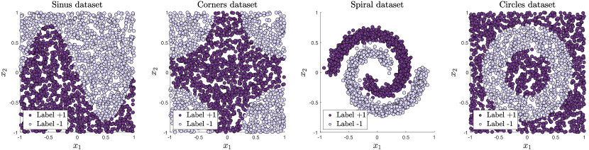
In this work we utilized four artificial datasets for evaluating the performance of the proposed embedded quantum kernels. Here we explain how they were created:

• Sinus Dataset: The sinus dataset is defined by a sinusoidal function, specifically $f(x_1)=-0.8\sin \left(\pi x_1\right)$. Points located above this sinusoidal curve are categorized as class -1, while points below it are assigned to class +1.

• Corners Dataset: The corners dataset comprises four quarters of a circumference with a radius of 0.75, positioned at the corners of a square. Points located inside these circular regions are labeled as class -1, while points outside are classified as class +1.

• Spiral Dataset: The spiral dataset features two spirals formed by points arranged along a trajectory defined by polar coordinates. The first spiral, denoted as class +1, originates at the origin (0, 0) and spirals outward in a counter-clockwise direction, forming a curve. The second spiral, labeled class -1, mirrors the first spiral but spirals inward in a clockwise direction. These spirals are generated by varying the polar angle, selected randomly to create the data points. The radial distance from the origin for each point depends on the angle, creating the characteristic spiral shape. Noise is added to the data points by introducing random perturbations to ensure they do not align perfectly along the spirals.

• Circles Dataset: The circles dataset is created using two concentric circles that define an annular region. The inner circle has a radius of $\sqrt{2/\pi }$, while the outer circle has a radius of $0.5\sqrt{2/\pi }$. Data points located within the annular region are labeled as -1, while those outside the region are labeled as +1.

Appendix G Numerical experiments

In the main we provide numerical results for two datasets for the $n$-to-$n$ and $1$-to-$n$ constructions up to 8 qubits. Here we provide the tables of more numerical experiments with the same hyperparameters: learning rate of 0.05 and 30 epochs for the $n=1$ QNN and learning rate of 0.005 and 10 epochs for $n>1$. Here we provide more results for different datasets and considering also CZ as source of entanglement. All accuracies refer to test accuracies.

Dataset	QNN accuracy	EQK type	EQK accuracy
Sinus	0.890	$3q$ $\mathrm{CNOT}$	0.960
Sinus		$3q$ $\mathrm{CZ}$	0.948
Corners	0.886	$3q$ $\mathrm{CNOT}$	0.954
Corners		$3q$ $\mathrm{CZ}$	0.940
Spiral	0.800	$3q$ $\mathrm{CNOT}$	0.994
Spiral		$3q$ $\mathrm{CZ}$	0.866
Circles	0.698	$3q$ $\mathrm{CNOT}$	0.866
Circles		$3q$ $\mathrm{CZ}$	0.864

Table 1: Numerical results for the $1$-to-$3$ architecture, considering two types of entangling gates ($\mathrm{CNOT}$ and $\mathrm{CZ}$), on four distinct datasets.

In Table 1, the outcomes demonstrate striking similarity when introducing entanglement through $\mathrm{CZ}$ gates or $\mathrm{CNOT}$ gates, with the exception of the spiral dataset. Given the ambiguity surrounding the method of entanglement introduction, one might contemplate utilizing controlled rotations with random parameters as a potential source of entanglement. Notably, it is observed that even starting from a single-qubit QNN achieving accuracies of less than $90\%$, the construction of EQKs yields accuracies surpassing $95\%$.

Figure G.1: Explicit quantum circuit for constructing the $1$-to-$3$ embedding quantum kernel with cascade of $CNOT$ gates as source of entanglement. The parameters ${𝜽}^{\ast }$ are the ones obtained during the training of the single-qubit QNN. Note that the parameters of the last layer are irrelevant.

Dataset	n=2	n=3	n=4	n=5	n=6	n=7	n=8	n=9	n=10
Corners	0.890	0.954	0.974	0.978	0.982	0.980	0.978	0.978	0.978
Circles	0.832	0.866	0.950	0.970	0.974	0.970	0.978	0.966	0.962

Table 2: Numerical results for the $1$-to-$n$ architecture for up to $n=10$ qubits. These results up to 8 qubits are depicted in the main text.

In the $1$-to-$n$ construction presented in Table 2 for the corners and circles datasets, we observe that the accuracy rises rapidly as qubits are added, reaching a peak at $n=4$. Subsequently, the accuracy plateaus, attaining a maximum at $n=6$ for the corners dataset and $n=8$ for the circles dataset. After reaching these points, the accuracy gradually decreases with additional qubits.

Dataset	n=1	n=2	n=3	n=4	n=5	n=6	n=7	n=8
Corners (QNN)	0.886	0.934	0.948	0.952	0.954	0.956	0.960	0.962
Corners (EQK)	0.898	0.948	0.960	0.966	0.970	0.972	0.974	0.974
Circles (QNN)	0.698	0.792	0.820	0.858	0.934	0.944	0.944	0.946
Circles (EQK)	0.796	0.820	0.906	0.968	0.974	0.974	0.976	0.980

Table 3: Numerical results for the $n$-to-$n$ architecture for up to $n=L+1=8$ qubits. These results are depicted in the main text.

In the $n$-to-$n$ approach, as presented in Table 3, the accuracy consistently increases with the addition of qubits for both the QNN and the EQK. Additionally, as discussed in the main text, the EQK consistently outperforms the corresponding QNN architecture for the same value of $n$.

Dataset	Layers	QNN accuracy	EQK accuracy
Sinus	$L=5$	0.948	0.970
Sinus	$L=6$	0.956	0.964
Sinus	$L=7$	0.966	0.972
Sinus	$L=8$	0.958	0.964
Corners	$L=5$	0.948	0.970
Corners	$L=6$	0.936	0.950
Corners	$L=7$	0.934	0.948
Corners	$L=8$	0.916	0.920
Spiral	$L=5$	0.952	0.996
Spiral	$L=6$	0.974	0.998
Spiral	$L=7$	0.978	1.000
Spiral	$L=8$	0.980	0.998
Circles	$L=5$	0.786	0.812
Circles	$L=6$	0.808	0.814
Circles	$L=7$	0.792	0.820
Circles	$L=8$	0.844	0.902

Table 4: Numerical results for the $2$-to-$2$ architecture for different number of layers. For the experiments in the main text we choose $L=7$.

Finally, in Table 4, we present results for the four datasets considering different numbers of layers for the $n$-to-$n$ architecture with $n=2$. Adding layers increases the expressivity of the QNN but does not guarantee better accuracies, as we can observe. Again, we see that the EQK consistently outperforms the QNN.

References

- Biamonte et al. (2017) J. Biamonte, P. Wittek, N. Pancotti, P. Rebentrost, N. Wiebe, and S. Lloyd, Nature 549, 195 (2017).
- Carleo et al. (2019) G. Carleo, I. Cirac, K. Cranmer, L. Daudet, M. Schuld, N. Tishby, L. Vogt-Maranto, and L. Zdeborová , Reviews of Modern Physics 91 (2019), 10.1103/revmodphys.91.045002.
- Dunjko and Briegel (2018) V. Dunjko and H. J. Briegel, Reports on Progress in Physics 81, 074001 (2018).
- Dalzell et al. (2023) A. M. Dalzell, S. McArdle, M. Berta, P. Bienias, C.-F. Chen, A. Gilyén, C. T. Hann, M. J. Kastoryano, E. T. Khabiboulline, A. Kubica, G. Salton, S. Wang, and F. G. S. L. Brandão, “Quantum algorithms: A survey of applications and end-to-end complexities,” (2023), arXiv:2310.03011 [quant-ph] .
- Benedetti et al. (2019) M. Benedetti, E. Lloyd, S. Sack, and M. Fiorentini, Quantum Science and Technology 4, 043001 (2019).
- Skolik et al. (2022) A. Skolik, S. Jerbi, and V. Dunjko, Quantum 6, 720 (2022).
- Schuld et al. (2020) M. Schuld, A. Bocharov, K. M. Svore, and N. Wiebe, Physical Review A 101 (2020), 10.1103/physreva.101.032308.
- Farhi and Neven (2018) E. Farhi and H. Neven, “Classification with quantum neural networks on near term processors,” (2018), arXiv:1802.06002 [quant-ph] .
- Sweke et al. (2021) R. Sweke, J.-P. Seifert, D. Hangleiter, and J. Eisert, Quantum 5, 417 (2021).
- Jerbi et al. (2021) S. Jerbi, L. M. Trenkwalder, H. Poulsen Nautrup, H. J. Briegel, and V. Dunjko, PRX Quantum 2 (2021), 10.1103/prxquantum.2.010328.
- Pirnay et al. (2023) N. Pirnay, R. Sweke, J. Eisert, and J.-P. Seifert, Physical Review A 107 (2023), 10.1103/physreva.107.042416.
- Gyurik and Dunjko (2023) C. Gyurik and V. Dunjko, “On establishing learning separations between classical and quantum machine learning with classical data,” (2023), arXiv:2208.06339 [quant-ph] .
- Havlíček et al. (2019) V. Havlíček, A. D. Córcoles, K. Temme, A. W. Harrow, A. Kandala, J. M. Chow, and J. M. Gambetta, Nature 567, 209 (2019).
- Schuld and Killoran (2019) M. Schuld and N. Killoran, Physical review letters 122, 040504 (2019).
- Pérez-Salinas et al. (2020) A. Pérez-Salinas, A. Cervera-Lierta, E. Gil-Fuster, and J. I. Latorre, Quantum 4, 226 (2020).
- Schuld et al. (2021a) M. Schuld, R. Sweke, and J. J. Meyer, Physical Review A 103 (2021a), 10.1103/physreva.103.032430.
- Caro et al. (2021) M. C. Caro, E. Gil-Fuster, J. J. Meyer, J. Eisert, and R. Sweke, Quantum 5, 582 (2021).
- Ono et al. (2023) T. Ono, W. Roga, K. Wakui, M. Fujiwara, S. Miki, H. Terai, and M. Takeoka, Physical Review Letters 131 (2023), 10.1103/physrevlett.131.013601.
- Jerbi et al. (2023) S. Jerbi, L. J. Fiderer, H. Poulsen Nautrup, J. M. Kübler, H. J. Briegel, and V. Dunjko, Nature Communications 14, 517 (2023).
- Huang et al. (2021) H.-Y. Huang, M. Broughton, M. Mohseni, R. Babbush, S. Boixo, H. Neven, and J. R. McClean, Nature Communications 12 (2021), 10.1038/s41467-021-22539-9.
- Peters et al. (2021) E. Peters, J. Caldeira, A. Ho, S. Leichenauer, M. Mohseni, H. Neven, P. Spentzouris, D. Strain, and G. N. Perdue, “Machine learning of high dimensional data on a noisy quantum processor,” (2021), arXiv:2101.09581 [quant-ph] .
- Bartkiewicz et al. (2020) K. Bartkiewicz, C. Gneiting, A. Černoch, K. Jiráková, K. Lemr, and F. Nori, Scientific Reports 10 (2020), 10.1038/s41598-020-68911-5.
- Kusumoto et al. (2021) T. Kusumoto, K. Mitarai, K. Fujii, M. Kitagawa, and M. Negoro, npj Quantum Information 7 (2021), 10.1038/s41534-021-00423-0.
- Schuld (2021) M. Schuld, arXiv preprint arXiv:2101.11020 (2021).
- Schuld et al. (2021b) M. Schuld, F. Petruccione, M. Schuld, and F. Petruccione, Machine Learning with Quantum Computers , 217 (2021b).
- Liu et al. (2021) Y. Liu, S. Arunachalam, and K. Temme, Nature Physics 17, 1013 (2021).
- Schölkopf and Smola (2001) B. Schölkopf and A. Smola, Smola, A.: Learning with Kernels - Support Vector Machines, Regularization, Optimization and Beyond. MIT Press, Cambridge, MA, Vol. 98 (2001).
- Vedaie et al. (2020) S. S. Vedaie, M. Noori, J. S. Oberoi, B. C. Sanders, and E. Zahedinejad, “Quantum multiple kernel learning,” (2020), arXiv:2011.09694 [quant-ph] .
- Ghukasyan et al. (2023) A. Ghukasyan, J. S. Baker, O. Goktas, J. Carrasquilla, and S. K. Radha, “Quantum-classical multiple kernel learning,” (2023), arXiv:2305.17707 [quant-ph] .
- Hubregtsen et al. (2022) T. Hubregtsen, D. Wierichs, E. Gil-Fuster, P.-J. H. S. Derks, P. K. Faehrmann, and J. J. Meyer, Physical Review A 106 (2022), 10.1103/physreva.106.042431.
- Abbas et al. (2021) A. Abbas, D. Sutter, C. Zoufal, A. Lucchi, A. Figalli, and S. Woerner, Nature Computational Science 1, 403–409 (2021).
- Cerezo et al. (2021) M. Cerezo, A. Sone, T. Volkoff, L. Cincio, and P. J. Coles, Nature Communications 12 (2021), 10.1038/s41467-021-21728-w.
- Bharti et al. (2022) K. Bharti, A. Cervera-Lierta, T. H. Kyaw, T. Haug, S. Alperin-Lea, A. Anand, M. Degroote, H. Heimonen, J. S. Kottmann, T. Menke, et al., Reviews of Modern Physics 94, 015004 (2022).
- Sharma et al. (2020) K. Sharma, S. Khatri, M. Cerezo, and P. J. Coles, New Journal of Physics 22, 043006 (2020).
- McClean et al. (2018) J. R. McClean, S. Boixo, V. N. Smelyanskiy, R. Babbush, and H. Neven, Nature Communications 9 (2018), 10.1038/s41467-018-07090-4.
- Holmes et al. (2022) Z. Holmes, K. Sharma, M. Cerezo, and P. J. Coles, PRX Quantum 3 (2022), 10.1103/prxquantum.3.010313.
- Anschuetz and Kiani (2022) E. R. Anschuetz and B. T. Kiani, Nature Communications 13 (2022), 10.1038/s41467-022-35364-5.
- Ragone et al. (2023) M. Ragone, B. N. Bakalov, F. Sauvage, A. F. Kemper, C. O. Marrero, M. Larocca, and M. Cerezo, “A unified theory of barren plateaus for deep parametrized quantum circuits,” (2023), arXiv:2309.09342 [quant-ph] .
- Buhrman et al. (2001) H. Buhrman, R. Cleve, J. Watrous, and R. de Wolf, Physical Review Letters 87 (2001), 10.1103/physrevlett.87.167902.
- Fanizza et al. (2020) M. Fanizza, M. Rosati, M. Skotiniotis, J. Calsamiglia, and V. Giovannetti, Physical Review Letters 124 (2020), 10.1103/physrevlett.124.060503.
- Cincio et al. (2018) L. Cincio, Y. Subaşı, A. T. Sornborger, and P. J. Coles, New Journal of Physics 20, 113022 (2018).
- Gil-Fuster et al. (2023) E. Gil-Fuster, J. Eisert, and V. Dunjko, arXiv preprint arXiv:2309.14419 (2023).
- Rebentrost et al. (2014) P. Rebentrost, M. Mohseni, and S. Lloyd, Physical review letters 113, 130503 (2014).
- Park et al. (2023) S. Park, D. K. Park, and J.-K. K. Rhee, Scientific Reports 13, 3288 (2023).
- Thanasilp et al. (2022) S. Thanasilp, S. Wang, M. Cerezo, and Z. Holmes, “Exponential concentration and untrainability in quantum kernel methods,” (2022), arXiv:2208.11060 [quant-ph] .
- Kübler et al. (2021) J. M. Kübler, S. Buchholz, and B. Schölkopf, “The inductive bias of quantum kernels,” (2021), arXiv:2106.03747 [quant-ph] .
- Lloyd et al. (2020) S. Lloyd, M. Schuld, A. Ijaz, J. Izaac, and N. Killoran, “Quantum embeddings for machine learning,” (2020), arXiv:2001.03622 [quant-ph] .
- Casas and Cervera-Lierta (2023) B. Casas and A. Cervera-Lierta, Physical Review A 107 (2023), 10.1103/physreva.107.062612.
- Barthe and Pérez-Salinas (2023) A. Barthe and A. Pérez-Salinas, “Gradients and frequency profiles of quantum re-uploading models,” (2023), arXiv:2311.10822 [quant-ph] .
- Pérez-Salinas et al. (2021) A. Pérez-Salinas, D. López-Núñez, A. García-Sáez, P. Forn-Díaz, and J. I. Latorre, Physical Review A 104 (2021), 10.1103/physreva.104.012405.
- Panadero et al. (2023) I. Panadero, Y. Ban, H. Espinós, R. Puebla, J. Casanova, and E. Torrontegui, “Regressions on quantum neural networks at maximal expressivity,” (2023), arXiv:2311.06090 [quant-ph] .
- Holmes and Jain (2006) D. E. Holmes and L. C. Jain, Innovations in machine learning (Springer, 2006).