A Closer Look at AUROC and AUPRC under Class Imbalance

Abstract

In machine learning (ML), a widespread claim is that the area under the precision-recall curve (AUPRC) is a superior metric for model comparison to the area under the receiver operating characteristic (AUROC) for tasks with class imbalance. This paper refutes this notion on two fronts. First, we theoretically characterize the behavior of AUROC and AUPRC in the presence of model mistakes, establishing clearly that AUPRC is not generally superior in cases of class imbalance. We further show that AUPRC can be a harmful metric as it can unduly favor model improvements in subpopulations with more frequent positive labels, heightening algorithmic disparities. Next, we empirically support our theory using experiments on both semi-synthetic and real-world fairness datasets. Prompted by these insights, we conduct a review of over 1.5 million scientific papers to understand the origin of this invalid claim, finding that it is often made without citation, misattributed to papers that do not argue this point, and aggressively over-generalized from source arguments. Our findings represent a dual contribution: a significant technical advancement in understanding the relationship between AUROC and AUPRC and a stark warning about unchecked assumptions in the ML community.

1 Introduction

Machine learning (ML), especially in critical domains like healthcare, necessitates carefully selecting and applying evaluation metrics to guide appropriate model choices and understand performance nuances (Hicks et al., 2022). Model evaluation can happen in one of two settings: (1) a methodological/model comparison setting, which occurs outside of a specific deployment setting and target model usage workflows, optimal decision thresholds, or specific false-positive (FP) and false-negative (FN) costs are typically not known, or (2) an application/deployment setting, where reasonably specific estimates of model usage workflows and FP/FN costs can be made. In both of these settings, appropriate evaluation metric choice is critical—inappropriate evaluation metrics can hinder innovation when used for model comparison and can lead to significant real world costs (e.g., mis-diagnosis in a medical setting) in deployment settings.

This study focuses on two pivotal metrics for binary classification tasks that are widely used in both evaluation contexts: the Area Under the Precision-Recall Curve (AUPRC) and the Area Under the Receiver Operating Characteristic (AUROC). Central to this paper is the following key claim:

Claim 1.

Let $f$ be a model which outputs continuous probabilistic predictions trained to solve a binary classification task for which the prevalence of negative labels is significantly higher than the prevalence of positive labels. For this problem, the AUPRC will yield a “better” or “more accurate” or “fairer” evaluation of $f$ than the AUROC.

Claim 1 is made widely in both the scientific literature (Wagner et al., 2023; Choi et al., 2018; Hsu et al., 2020; Gong et al., 2021) and in popular press sources (Czakon, 2022; Mazzanti, 2023) and has been justified on numerous grounds (See sources collated in the literature review in Section 5). Despite this, we show in this work that this claim is, in fact, wrong, and many of its justifications are invalid or misapplied in common ML settings. More specifically, we show the following:

1) AUROC and AUPRC only differ with respect to model-dependent parameters in that AUROC weighs all false positives equally, whereas AUPRC weighs false positives at a threshold $\tau$ with the inverse of the model’s likelihood of outputting any scores greater than $\tau$ (Theorem 1). This result shows that we can reason about the suitability of optimizing or selecting by AUROC vs. AUPRC on the basis of whether we care more about reducing false positives above low thresholds or high thresholds. In particular,

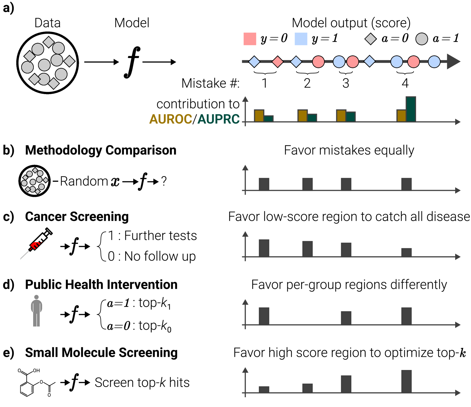
2) AUROC favors model improvements uniformly over all positive samples, whereas AUPRC favors improvements for samples assigned higher scores over those assigned lower scores (Theorem 2). This indicates that the key factor differentiating the utility of AUROC or AUPRC as an evaluation metric is not class imbalance at all, but it is rather based on the target use case of the model in question. See Figure 1 for a visual explanation. It also reveals that AUPRC can amplify algorithmic biases. In particular,

3) AUPRC can unduely prioritize improvements to higher-prevalence subpopulations at the expense of lower-prevalence subpopulations, raising serious fairness concerns in any multi-population use cases (Theorem 3).

In this work, we will establish these three claims theoretically, via synthetic experiments, and with real-world validation on popular public fairness datasets. We will additionally demonstrate through an extensive, large-language model aided literature review of over 1.5 million scientific papers, that Claim 1 has been used to motivate numerous improper uses of AUPRC relative to AUROC across high-impact domains like healthcare in a range of well known venues, including Cancer Cell, Nature Scientific Reports, AAAI, and NeurIPS. Through this paper, we hope to shed greater light on the nuances of appropriate evaluation and provide key guidance to limit future misuse of evaluation metrics in the scientific and machine learning communities.

Figure 1: a) Consider a model $f$ yielding continuous output scores for a binary classification task applied to a dataset consisting of two distinct subpopulations, $𝒜\mathrm{\in }\mathrm{\{}\mathrm{0}\mathrm{,}\mathrm{1}\mathrm{\}}$ (e.g., race). If we order samples in ascending order of output score, we define a mistake to be when two neighboring samples are out-of-order with respect to the classification label (such as Mistake 1, 2, 3, and 4 in the figure). Each such mistake represents an unambiguous, indivisible opportunity for model improvement; namely, swap the out-of-order samples, and the model will improve. Under any such swapping operation, the model’s AUROC will improve by the same amount, while the model’s AUPRC will improve by an amount correlated with the inverse of the number of samples the model assigns a higher score than the samples in the mistake (Theorem 2). b) If we are performing model comparison outside of a deployment setting, the we will have no insight into the expected costs of various kinds of mistakes and we have no reason to believe we will primarily be concerned with samples $x$ that are drawn from any particular region in the model output space. Therefore, in this setting, an appropriate model evaluation metric should improve by the same amount regardless of which mistake is corrected. c) In a deployment setting where false negatives have a high cost relative to false positives, such as a routine screening test for a serious disease like cancer, then an appropriate evaluation metric should optimize for ensuring that we can most efficiently catch all cases of the disease and minimize the number of false negatives. This corresponds to favoring mistakes that have lower scores, regardless of the fact that many such tasks have significant rates of class imbalance. d) In a deployment setting where a limited number of key resources will be distributed among members of a large population, in a manner that requires certain subpopulations to be offered commensurate possible benefit from the intervention for ethical reasons, a proper evaluation metric should prioritize the importance of within-group, high-score mistakes such that the highest risk members of each subgroup can receive the limited number of interventions. e) In a deployment setting where false positives are expensive relative to false negatives and there are no fairness concerns, such as prioritizing small molecule leads for drug development, where the top $k$ most likely molecules will be presented for expensive follow-up experimental validation, appropriate evaluation should favor model improvements in decreasing order with score, to maximize the likelihood of successfully identifying appropriate molecules among the limited set of $k$ selections.

2 Theoretical Analyses

2.1 Relationship Between AUROC and AUPRC

In this section, we introduce Theorem 1, which is as follows:

Theorem 1.

Let $f\mathrm{:}𝒳\mathrm{\to }\mathrm{(}\mathrm{0}\mathrm{,}\mathrm{1}\mathrm{)}$ be a binary classification model over a data distribution $𝗑\mathrm{,}𝗒$ of model inputs $x\mathrm{\sim }𝗑\mathrm{,}x\mathrm{\in }𝒳$ and labels $y\mathrm{\sim }𝗒\mathrm{,}y\mathrm{\in }\mathrm{(}\mathrm{0}\mathrm{,}\mathrm{1}\mathrm{)}$. Then,

$\mathrm{AUROC}(f)$ $=1-{𝔼}_{t\sim f(𝗑)|𝗒=1}\left[\mathrm{FPR}(f,t)\right]$

$\mathrm{AUPRC}(f)$ $=1-p_{𝗒}(0){𝔼}_{t\sim f(𝗑)|𝗒=1}\left[{\displaystyle \frac{\mathrm{FPR}(f,t)}{P(f(𝗑)>t)}}\right]$

We provide the proof in Appendix Section C. The two key intuitions are that integrating over the TPR is equivalent to taking the expectation over the induced distribution of positive sample scores, and that via Bayes rule, $\mathrm{Prec}(f,\tau )=1-p_{𝗒}(0)\frac{\mathrm{FPR}(f,\tau )}{P(f(𝗑)>\tau )}$.

Despite its simplicity, Theorem 1 has far-reaching implications. Namely, it reveals that the only difference between AUROC and AUPRC with respect to model dependent parameters (i.e., omitting the dependence of AUPRC on the fixed prevalence of the dataset, which is not model varying) is that optimizing AUROC equates to minimizing the expected false positive rate over all positive samples in an unweighted manner (equivalently, in expectation over the distribution of positive sample scores) whereas optimizing AUPRC equates to minimizing the expected false positive rate over all positive samples weighted by the inverse of the model’s “firing rate” ($P(f(𝗑)>\tau )$) at the given positive sample score. This preference can be crystallized when we examine how AUROC vs. AUPRC would prioritize correcting indivisible units of model improvements, termed “mistakes” which we will discuss next.

2.2 AUPRC prioritizes high-score mistakes, AUROC treats all mistakes equally

Understanding how a given evaluation metric prioritizes the correction of various kinds of model mistakes or errors offers significant insight into when that metric should be used for optimization or model selection. To examine this topic for AUROC and AUPRC, consider the following definition of a model “mistake”:

Definition 2.1.

Let $f:𝒳\to (0,1)$ be a binary classification model over a domain $𝒳$ being evaluated over a static, finite dataset $𝑿,𝒚=\{(x_1,y_1),\mathrm{\dots },(x_N,y_N)\}$, for $x_i\in 𝒳,y_i\in \{0,1\},$ and $N\in \mathbb{N}$. We assume for convenience that $f$ is an injective map and all $x_i$ are distinct (i.e., $\forall (i,j):f(x_i)\ne f(x_j)$).

We say that a model makes a mistake at samples $(x_i,x_j)$ if:

1. $y_i=1$ and $y_j=0$

3. $\mathrm{\nexists }{x}_k$ such that .

Essentially, Definition 2.1 states that a mistake occurs when a model assigns adjacent probability scores to a pair of samples with discordant labels, as shown in Figure 1. With this in mind, we can then introduce Theorem 2 which states that AUROC improves by a constant amount regardless of which mistake is corrected for a given model and dataset whereas AUPRC improves more when the mistake corrected occurs at a higher score than when it occurs at a lower score:

Theorem 2.

Define $f\mathrm{,}𝒳\mathrm{,}𝐗\mathrm{,}𝐲$ and $N$ as in Definition 2.1. Further, suppose without loss of generality that the dataset $𝐗$ is ordered such that for all $i$. Then, let us define $M\mathrm{=}\mathrm{\{}i\mathrm{|}\mathrm{(}{x}_i\mathrm{,}{x}_{i\mathrm{+}\mathrm{1}}\mathrm{)}\mathit{}\mathit{\text{is a}}\mathrm{\text{mistake}}\mathit{\text{for model}}f\mathrm{\}}$. Define $f_i^{\mathrm{\prime }}$ to be a model that is identical to $f$ except that the probabilities assigned to $x_i$ and $x_{i\mathrm{+}\mathrm{1}}$ are swapped:

Then, $\mathrm{AUROC}\mathit{}\mathrm{(}{f}_i^{\mathrm{\prime }}\mathrm{)}\mathrm{=}\mathrm{AUROC}\mathit{}\mathrm{(}{f}_j^{\mathrm{\prime }}\mathrm{)}$ for all $i\mathrm{,}j\mathrm{\in }M$, and for all $i\mathrm{,}j\mathrm{\in }M$ such that .

The proof for Theorem 2 can be found in Appendix D. This proof simply stems from the fact that correcting a single mistake $(x_i,x_j)$ (as defined in Definition 2.1) always changes the false positive rate by the same amount, and only changes it at the threshold $f(x_i)$. This, combined with the formalization of AUROC and AUPRC in Theorem 1, establishes the proof.

2.3 AUPRC is explicitly discriminatory in favor of high-scoring subpopulations

The reliance on a model’s firing rate revealed in Theorem 1 and the optimization behavior in Theorem 2 reveals significant issues with the fairness of AUPRC. In particular, in this section we introduce Theorem 3:

Theorem 3.

Let $f\mathrm{,}𝒳\mathrm{,}𝐗\mathrm{,}𝐲\mathrm{,}N\mathrm{,}M\mathrm{,}$ and $f_j^{\mathrm{\prime }}$ all be defined as in Theorem 2. Further, suppose that in this setting the domain $𝒳$ now contains an attribute defining two subgroups, $𝒜\mathrm{=}\mathrm{\{}\mathrm{0}\mathrm{,}\mathrm{1}\mathrm{\}}$, such that for any sample $\mathrm{(}{x}_i\mathrm{,}{y}_i\mathrm{)}$, $a_i$ denotes the subgroup to which that sample belongs. Let $f$ be perfectly calibrated for samples in subgroup $a\mathrm{=}\mathrm{0}$, such that $p_{𝗒\mathrm{|}𝖺\mathrm{=}\mathrm{0}\mathrm{,}f\mathit{}\mathrm{(}𝗑\mathrm{)}\mathrm{=}t}\mathit{}\mathrm{(}\mathrm{1}\mathrm{)}\mathrm{=}t$. Let $p_{\mathrm{0}}\mathrm{=}{p}_{𝗒\mathrm{|}𝖺\mathrm{=}\mathrm{0}}\mathit{}\mathrm{(}\mathrm{1}\mathrm{)}$ denote the prevalence of the label $y$ over subgroup $a\mathrm{=}\mathrm{0}$. Then,

$$\underset{p_0\to 0}{lim}P(a_i=a_{i+1}=1|i=\underset{j\in ℳ}{\arg \max }\left(\mathrm{AUPRC}(f_j^{\prime })\right))=1.$$

Essentially, Theorem 3 (proof provided in Appendix E) shows that for any model of interest, provided the model is calibrated, there exists a prevalence disparity sufficiently severe such that the likelihood of the mistake occurring with highest score (which will maximally improve AUPRC) belonging to anything other than the high prevalence subgroup goes to zero. This demonstrates that AUPRC provably favors higher prevalence subpopulations under sufficiently severe class imbalance.

Note that this property is, generally speaking, not desirable. In particular, this property establishes that in settings where model fairness among a set of subpopulations in the data is important, AUPRC should not be used as an evaluation metric due to the risk that it will introduce biases in favor of the highest prevalence subpopulations. We validate this result empirically over both synthetic and real-world data in Section 3, demonstrating that the import of Theorem 3 is not merely limited to an analytical curiosity but can have real world impact on algorithmic disparities in practice.

Furthermore, note that this theorem does not indicate that AUPRC will be superior to AUROC for differentiating a low prevalence (or low risk) subpopulation relative to a high-risk subpopulation, a property that is sometimes attributed to AUPRC in the literature. Rather, Theorem 3 shows that maximizing AUPRC will be more likely to optimize solely within the high-risk subgroup, rather than optimizing to differentiate across subgroups, as low-risk subgroup samples will only occur in lower-score regions under severe class imbalance.

3 Experimental Validation

In this section, we establish via synthetic and real-world experiments that Theorem 3 is not merely an analytical effect but has real world consequences on the implications of optimizing or performing model selection via AUPRC.

3.1 Synthetic Optimization Experiments Demonstrate AUPRC-induced Disparities

Experimental Setup.

Let $Y\in \{0,1\}$ be the binary label, $S\in [0,1]$ be the predicted score, and $G\in \{G_1,G_2\}$ be the subpopulation. We fix $\mathbb{P}(Y=1|G=G_1)=0.05$ and $\mathbb{P}(Y=1|G=G_2)=0.01$. We sample a dataset for each group ${𝒟}_g=\{(S_1,Y_1),\mathrm{\dots },(S_{n_g},Y_{n_g})\}$, such that $\text{AUROC}({𝒟}_1)\approx \text{AUROC}({𝒟}_2)\approx \text{AUROC}({𝒟}_1\cup {𝒟}_2)=0.85$ (A target AUROC of 0.65 was also profiled in Appendix Figure 5).

Our main experimental challenge is to determine how to simulate “optimizing” or “selecting” a model by AUROC or AUPRC. We explore two approaches here. First, we can simply correct the atomic mistake that maximally improves AUROC or AUPRC in each optimization iteration. In our experiments, we use $n_1=n_2=200$ and optimize for $50$ steps for this experiment. This is the most straightforward optimization procedure to analyze, but it is unrealistic. In real optimization scenarios, larger model changes will be made at once, and a model will have an opportunity to degrade performance in some regions in order to improve it in others.

Next, we profile an optimization procedure that randomly permutes all the (sorted) model scores up to 3 positions. This has the effect of randomly adjusting all model scores, and can worsen model performance under some random permutations, but offset precisely the same capacity to the low and high prevalence subgroups. To ensure the model is under some optimization constraint (and therefore does not always find the “perfect” permutation to maximize both metrics identically), we allow the model to sample only 15 possible permutations before choosing the best option. This means the system will be forced to navigate optimization trade-offs between which permutations improve the right regions of the score most effectively among its limited set. We use $n_1=n_2=100$ for these experiments and optimize for $25$ total steps.

Figure 2: Synthetic experiment per-group AUROC after successively either fixing individual mistakes, as defined in Definition 2.1, (a) and b)) or successively choosing the optimal score permutation (c) and d)) in order to optimize either AUROC (a) and c)) or AUPRC (b) and d)). It is clear across both forms of optimization that AUPRC definitively favors the higher prevalence subpopulation, whereas AUROC treats subgroups approximately equally. Similar patterns were observed when comparing per-group AUPRCs over the same experimental procedures, as shown in Appendix Figure 4.

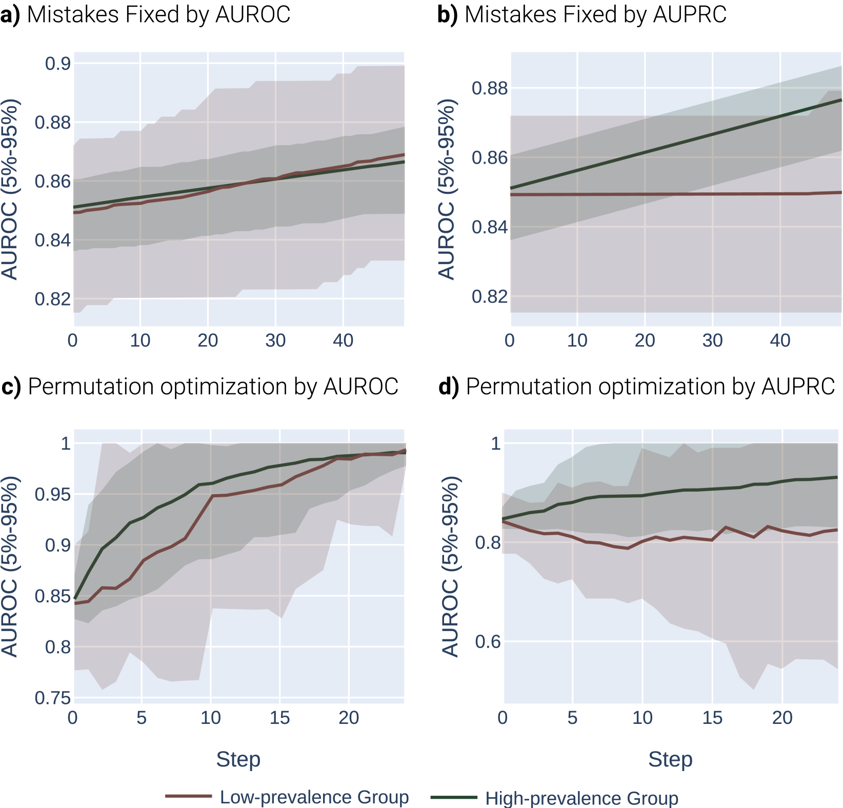
Across both settings, we run these experiments across 20 randomly sampled datasets and show the mean and an empirical 90% confidence interval around the mean in Figure 2. We present a formal mathematical formulation of these perturbations, as well as profile a third random perturbation method, in Appendix F.3.

Results.

Our results demonstrate the impact of the optimization metric on subpopulation disparity. In particular, in Figure 2, we observe a notable disparity introduced when optimizing under the AUPRC metric regardless of the optimization procedure. This is evident in the performance metrics across the high and low prevalence subpopulations, which exhibit significant divergence as the optimization process favors the group with higher prevalence. In the more realistic, random-permutation optimization procedure (Figure 2d), this even results in a decrease in the AUROC for the low prevalence subgroup. In comparison, when optimizing for overall AUROC, the AUROC of both groups increase together. Note that we show the effect of this optimization on the AUPRC metric, which shows very similar trends, in Appendix Figure 4.

3.2 Real-World Experimental Validation

To demonstrate the generalizability of our finding to the real world, we evaluate fairness gaps induced by AUROC and AUPRC selection on four common datasets in the fairness literature (Zhang et al., 2018; Fabris et al., 2022; Lahoti et al., 2020).

Datasets.

We use the following four tabular binary classification datasets: adult (Asuncion & Newman, 2007), compas (Angwin et al., 2022), lsac (Wightman, 1998), and mimic (Johnson et al., 2016). In each dataset, we consider both sex and race as sensitive attributes. To mimic the setting of our theorems, we balance each dataset by the sensitive attribute during both training and test, by randomly subsampling the majority group. Further details about each dataset, as well as preprocessing steps, can be found in Appendix G.

Experimental Setup.

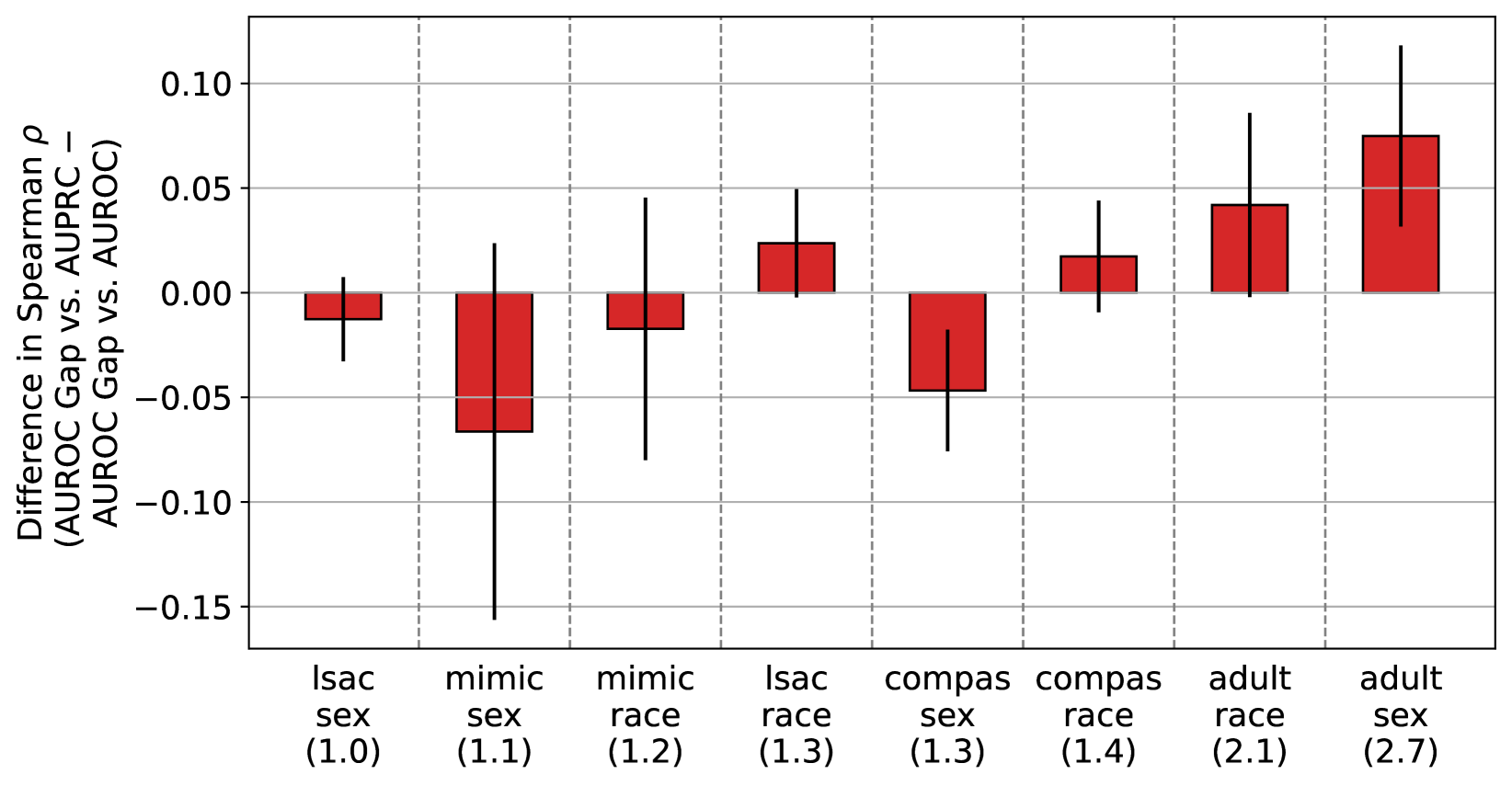
We train XGBoost models (Chen & Guestrin, 2016) on each dataset. For each task, we iterate over a grid of per-group weights in order to create a diverse set of models that favor different groups. For each setting of task and per-group weight, we conduct a random hyperparameter search (Bergstra & Bengio, 2012) with 50 runs. We evaluate the validation set overall AUROC and AUPRC. We also evaluate the test set AUROC gap and AUPRC gap between groups, where gaps are defined as the value of the metric for the higher prevalence group minus the value for the lower prevalence group. Based on our theorems, our hypothesis is that overall AUPRC should be more positively correlated with the signed AUROC gap than overall AUROC, indicating that it better favors the higher prevalence group, especially when the prevalence ratio between groups is high. To test this hypothesis, we evaluate the Spearman correlation coefficient between these quantities. We repeat this experiment 5 times, with different random data splits, to obtain a 95% confidence interval.

Figure 3: Difference in the Spearman’s $\rho$ between the test-set signed AUROC gap versus the validation set overall AUPRC, and the AUROC gap versus the overall AUROC. Numbers in parentheses are the prevalence ratios between the two groups for the particular attribute, and datasets are sorted by this quantity. Error bars are 95% confidence intervals from five different random data splits.

Results.

In Figure 3, we plot the difference in the Spearman correlation coefficient of the AUROC gap versus the overall AUPRC, and AUROC gap versus overall AUROC. We observe mixed results in datasets with low prevalence ratio. In dataset with higher prevalence ratio, we find that overall AUPRC is more positively correlated with the AUROC gap than overall AUROC, indicating that AUPRC more favors the higher prevalence group. We emphasize that the prevalence ratios observed in these real-world datasets is much lower than the ratio of 5 used in our synthetic experiments, which may account for the mild effect observed. To see raw results from these experiments, see Appendix Figure 7.

Next, in Appendix Figure 8, we plot the difference in the Spearman’s $\rho$ from Figure 3, versus the prevalence gap. We find that there is a statistically significant correlation between the two (Spearman’s $\rho$ = 0.714, p = 0.047). Thus, while our power to detect a prevalence mediated AUPRC bias amplification effect is limited due to the limited prevalence disparities in these datasets, we nonetheless observe a strong positive correlation between the extent of the prevalence mismatch between the low and high prevalence group and the amount that AUPRC favors the high prevalence group over AUROC. In other words, our results show that across these fairness datasets and attributes, as the prevalence disparity grows more extreme, we observe a statistically significant corresponding increase in the extent to which AUPRC introduces algorithmic bias, exactly in accordance with what Theorem 3 suggests.

4 If not for class imbalance, then when should we use AUPRC vs. AUROC?

In Sections 2 and 3, we have shown that AUPRC is not universally superior in cases of class imbalance (and that instead it merely preferentially optimizes high-score regions over low-score regions) and that it also poses serious risks to the model fairness in settings where subgroup prevalences differ. In light of this, how should we revise Claim 1 to reflect when we actually should use AUPRC instead of AUROC or vice versa?

In this section, we explore this question, and provide practical guidance on metric selection. We build on our existing theoretical results and argue that the decision to utilize the AUROC or the AUPRC as the metric for evaluating binary classification models is intricately linked to the specific context in which the model operates, including the relative impact of false positives versus false negatives and the planned model workflow in deployment settings. To demonstrate this, here we return to the four example problems first depicted in Figure 1:

For context-independent model evaluation, use AUROC:

For model evaluations conducted outside of specific deployment contexts, where the differential costs of errors are undefined, the necessity for a metric that impartially values improvements across the entire model output space becomes paramount. As shown in Figure 1a, in this setting, as it is not known in advance where samples of interest will live in the output space nor are particular cost ratios known, correcting any model mistake should be prioritized equally to any other. This scenario inherently advantages AUROC, attributing to its capacity to uniformly account for every correction, thereby offering a comprehensive assessment of model performance irrespective of decision thresholds.

For deployment scenarios with elevated false negative costs, use AUROC:

In applications where the consequences of false negatives are especially grave, such as in the early screening for critical illnesses like cancer (refer to Figure 1c), the primary focus of the model in use will be to ensure that as few positive samples are missed as possible. This equates to prioritizing model recall. In such a scenario, the most important mistakes to correct are actually those that occur at lower score thresholds, because high-score mistakes will not change which positive samples are missed in deployment settings as chosen thresholds are likely to be low. This behavior is the inverse of what AUPRC prioritizes, demonstrating that in such situations, AUROC should be preferred over AUPRC. This choice will better ensure a reduction in false negatives, enhancing the model’s proficiency in detecting all possible disease instances.

For ethical resource distribution among large populations, use AUROC:

When faced with the challenge of ethically allocating scarce resources across a broad population, necessitating equitable benefit distribution among subgroups (illustrated in Figure 1d), it is crucial to avoid prioritizing model improvements that selectively favor one subpopulation. As AUPRC will target high-score regions selectively, it risks unduely favoring high-prevalence subpopulations, as shown in Theorem 3 and Figures 2 and 3. Even though in this resource distribution problem, high-score regions are selectively important compared to low-score regions, the fact that in this problem, we must prioritize across all subpopulations equally means that AUPRC’s global preference is untenable as it could induce bias. Thus, as shown in Figure 1d, we should prefer AUROC in this scenario as it will ensure uniform preference across groups, even though it prioritizes both low and high-score regions within each group.

For reducing false positives in high-cost, single-group intervention prioritization or information retrieval settings, use AUPRC:

In scenarios where the cost associated with false positives significantly outweighs that of false negatives, absent of equity concerns—such as in selecting candidate molecules from a fragment library for drug development trials, where only the most promising molecules will proceed to costly experimental validation (Figure 1e)—the metric of choice should facilitate a reduction in high-score false positives. This necessitates a focus on correcting high-score errors, for which AUROC might not be ideal due to its uniform treatment of errors across the score spectrum, potentially obscuring improvements in critical high-stake decisions.

5 If AUPRC is not better than AUROC under class imbalance, why did we think it was?

Claim 1, which states that “AUPRC is better than AUROC in cases of class imbalance” is widespread in the literature. Via both a manual literature search and an automated search of over 1.5M arXiv papers (see Appendix H for methodology), we observed 128 publications making this claim. We analyzed these papers to answer the following two key questions: (1) how has this incorrect claim become so widespread in ML and (2) has this claim led to inappropriate usage of evaluation metrics in high-impact settings?

5.1 Finding 1: This claim is often made without attribution or with inappropriate attribution.

This claim is frequently stated without any citation.

Among the 128 papers we discovered referencing this claim, 31 did so with no associated citation (Liu et al., 2023; Randl et al., 2023; Tusfiqur et al., 2022; Piermarini et al., 2023; Zhang & Bondell, 2018; Torfi et al., 2022; Wu et al., 2020; Navarro et al., 2022; Wagner et al., 2023; Herbach, 2021; Si & Roberts, 2021; Narayanan et al., 2022; Rayhan et al., 2017; Yang et al., 2022a, b; Harer et al., 2018; Lee et al., 2020; Zavrtanik et al., 2021; Rezvani et al., 2021; Prapas et al., 2023; Thambawita et al., 2020; Vijayan et al., 2017; Brophy & Lowd, 2020; Lyu et al., 2021; Chakraborty et al., 2023; Rajabi & He, 2021; Kim et al., 2022; Kiran et al., 2018; Mousavian et al., 2016; Rohani & Eslahchi, 2019; Rao et al., 2022). These papers were published in venues ranging from arXiv only to Nature Scientific Reports, ICCV, ECCV, and Bioinformatics, among others. This reflects not only the widespread belief in this claim, but also that we may be too comfortable making seemingly “correct” assertions without appropriate attribution in ML today.

This claim is frequently attributed to papers that do not make this claim.

Among the 97 that reference this claim and cite a source for this assertion, 39 do not cite any papers that make this claim in the first place (Yang et al., 2015; Li et al., 2020; Kyono et al., 2018; Seo et al., 2021; Hong et al., 2019; Hagedoorn & Spanakis, 2017; Babaei et al., 2021; Zou et al., 2022; Mangolin et al., 2022; Mosteiro et al., 2021; Showalter & Wu, 2019; Cranmer & Desmarais, 2016; Bryan & Moriano, 2023; Zhang et al., 2017; Domingues et al., 2020; Shukla & Marlin, 2019; Blevins et al., 2021; Hsu et al., 2020; Smith et al., 2023; Chu et al., 2018; Deshwar et al., 2015; Mongia et al., 2021; Rubin et al., 2012; Ahmed & Courville, 2020; Gong et al., 2021; Shukla & Marlin, 2018; Ma et al., 2022; Lei Ba et al., 2015; Newby et al., 2022; Ando & Huang, 2017; Stolman et al., 2022; Won et al., 2019; Stephenson et al., 2022; Srivastava et al., 2019; Karadzhov et al., 2022; Vens et al., 2008; López et al., 2013; Hall et al., 2023; Goyal & Khiari, 2020). In total, 13 sources are cited that neither reference nor argue this claim (Davis & Goadrich, 2006; Branco et al., 2016; Provost & Fawcett, 1997; Sokolova & Lapalme, 2009; Wahid-Ul-Ashraf et al., 2019; Ezzat et al., 2017; Burez & Van den Poel, 2009; Flach et al., 2011; Krawczyk, 2016; He & Garcia, 2009; LCT14558, 2017; Lobo et al., 2008). Most often, papers erroneously attribute this claim to Davis & Goadrich (2006), which was cited as a source for this claim 47 times. While Davis & Goadrich (2006) makes many interesting, meaningful claims about the ROC and PR curves, and does argue that the precision-recall curve is more informative than the ROC in cases of class imbalance it never asserts that the area under the PR curve should be preferred over the area under the ROC in cases of class imbalance. It references the emergence of the use of AUPRC instead of or in addition to the AUROC in this context, citing among those references a paper that would later be re-published as (Goadrich et al., 2006), which does make this claim, but (Davis & Goadrich, 2006) itself makes no claim about whether or not AUPRC should be preferred in this way, even by proxy to those prior references. The fact that, despite this, it receives so much citation volume for this claim reflects poorly on the accuracy of our scientific discourse in ML today.

Arguments associated with this claim frequently over-generalize the applicability of this claim or are biased by the appearance of metric superiority rather than true metric utility.

As noted in Section 4, there are real world settings in which AUPRC is more aligned with real-world usage than is AUROC (e.g., in a single-group, top-$k$ retrieval setting). However, Claim 1 is often made as a statement about all settings featuring class imbalance. Given this over-generalization, it is unsurprising that many arguments presented in favor Claim 1 when it is used in the literature are similarly over-generalized beyond the cases in which they would be appropriate. For example, claims such as that “precision-recall curves are more informative of deployment metrics” are often used to justify why AUPRC should be used in all cases of class imbalance, rather than just in cases where the relevant deployment metrics are most directly associated with the PR curve. Another class of arguments made in favor of Claim 1 can be reduced to arguments that the metric AUROC is poor in cases of class imbalance because the scores it produces are misleadingly high. While this argument can reflect a meaningful limitation of the communication value of the AUROC, comments about singleton metric results (rather than model comparison through metric values) are inherently orthogonal to the goal of model evaluation. In other words, what matters for model evaluation is not how high a given metric is, but rather the extent to which the metric meaningfully captures the right improvements in the model in the right ways. For a full breakdown of the arguments we observed in the literature and the sources making them, see Appendix Tables 2 and 3.

5.2 Finding 2: Claim 1 has led to inappropriate evaluation usage across a variety of high impact settings and in high-impact publication venues

We find that Claim 1 has been used to justify the use of AUPRC in a variety of settings where AUROC would actually be a superior evaluation metric, in high-impact domains including healthcare and safety, across high-impact venues including NeurIPS, AAAI, Cancer Cell, Nature Scientific Reports, Briefings in Bioinformatics, and Critical Care Medicine, among others. Many of the papers in question here have been cited numerous times, further underscoring the potential negative impact erroneous metric choices in these sources could have. These sources include the following works: (Wagner et al., 2023; Yuan et al., 2015; Lim & van der Schaar, 2018; Leisman, 2018; Cho et al., 2021; Kyono et al., 2018; Yang et al., 2022b; Meister et al., 2022; Mosteiro et al., 2021; Hashemi et al., 2018; Ozyegen et al., 2022; Thambawita et al., 2020; Hsu et al., 2020; Choi et al., 2018; Tiulpin et al., 2019; Lopez-Martinez et al., 2022; Gong et al., 2021; Moor et al., 2019; Ding et al., 2018).

For a representative example of these works, consider Wagner et al. (2023), in which the authors use ML methods to predict colorectal cancer status from medical imaging data. They suggest the following workflow for their model “Our intended clinical use of this workflow is as follows… First, a patient attends a clinic either with suspected CRC or for routine CRC screening. A colonoscopy shows a suspicious tumor, which is evaluated histologically and found to be an adenocarcinoma… Because of its high sensitivity, our algorithm could serve as a filtering step followed by affirmative testing for MSI-high predicted cases. Applying AI-based biomarker prediction would reduce the additional testing burden and therefore speed up the step between taking the biopsy and the molecular determination of MSI-high status, thus enabling an earlier treatment with immunotherapy if indicated.” Under this workflow, two things are clear: (1) the cost of a false positive in this setting is comparatively lower than a false negative, as a false positive only results in unnecessary “molecular determination of MSI-high status” whereas a false negative results in a delay of treatment with immunotherapy, and (2) as motivated by this cost ratio, the model is appropriately designed for (and achieves) a high sensitivity (a.k.a. recall).

As illustrated visually in Figure 1 and argued from first principles through our theoretical analyses in Sections 2 and 4, in this setting given points 1 and 2 above, AUPRC is very much not the right metric to use, precisely because it will favor improvements in high-score regions that will optimize precision rather than those in low-score regions that will help minimize false negatives. Despite this, the authors of this work, as motivated by Claim 1’s extensive publication history, explicitly use AUPRC over AUROC in this setting due to the class imbalance of their problem. This demonstrates the real-world negative impact that the spread of Claim 1 has had in the scientific community.

6 Limitations and Future Works

While our analyses are thorough and compelling, there are still a number of areas for further improvement and future work. Firstly, our theoretical findings can be refined and generalized to less restrictive settings, that take into account the difficulty of the target task (which may differ between subgroups) or does not require models to be calibrated (in the case of Theorem 3). Further, extending our real-world experiments to more fairness datasets and identifying more nuanced ways to probe the impact of metric choice on disparity measures would significantly strengthen this work. Lastly, These analyses can be extended to consider other metrics, such as the area under the precision-recall-gain curve (Flach & Kull, 2015), the area under the net benefit curve (Talluri & Shete, 2016; Pfohl et al., 2022), and single-threshold, deployment centric metrics as well.

7 Conclusion

This study rigorously interrogates the pervasive assumption within the machine learning community that AUPRC is a more appropriate evaluation metric than AUROC in class-imbalanced settings. Our empirical analyses, along with an exhaustive literature review, have revealed several important findings that critically challenge this belief. In particular, we show that while optimizing for AUROC equates to minimizing the model’s FPR in an unbiased manner over positive sample scores, optimizing for AUPRC equates to minimizing the FPR specifically for regions where the model outputs higher scores relative to lower scores. We further show both theoretically and empirically over synthetic and real-world fairness datasets that AUPRC can be an explicitly discriminatory metric in that it favors higher-prevalence subgroups.

In summary, our research advocates for a more thoughtful and context-aware approach to selecting evaluation metrics in machine learning. This paradigm shift, favoring a balanced and conscientious approach to metric selection, is essential in advancing the field towards developing not only technically sound, but also equitable and just models.

Broader Impact and Ethical Considerations

This research paper challenges the conventional wisdom regarding the superiority of the AUPRC over AUROC in binary classification tasks with class imbalance and has several ethical implications and impacts.

Our analysis reveals that the preference for AUPRC in certain ML applications may not be empirically justified and could inadvertently amplify algorithmic biases. This calls for a re-examination of prevalent metrics within ML, especially in high-stakes domains like healthcare, finance, and criminal justice where biased models can have profound societal repercussions. The tendency of AUPRC to disproportionately favor models with higher prevalence of positive labels could exacerbate existing disparities, underscoring the ethical need for rigorous validation and scrutiny of evaluation metrics.

Additionally, our use of large language models for literature analysis demonstrates a novel approach in scrutinizing and re-evaluating long-standing assumptions in ML. This method could set a precedent for more comprehensive and robust scientific investigations in the field, fostering a culture of empirical rigor and ethical awareness.

The ethical dimension of our work lies in the spotlight it casts on metric selection in ML model evaluation. The potential of metrics like AUPRC to skew model performance favoring certain groups raises pressing concerns about fairness in algorithmic decision-making. This is particularly critical when algorithms influence key decisions affecting individuals and communities.

While we use the COMPAS dataset for recividism prediction in this work, we recognize the many societal issues with automated predictions of recidivism (Dressel & Farid, 2018). We utilize this dataset as it is a commonly used dataset in the fairness literature, but do not advocate for deployment of these models in any way.

Our study contributes to the technical discourse on metric behaviors in ML and serves as a cautionary tale against uncritically embracing established norms. It underscores the imperative for careful metric selection aligned with ethical principles and fairness objectives in ML, highlighting the far-reaching consequences of these choices in shaping societal outcomes and advancing the field of ML.

Appendix A Code Availability

All code is available at https://github.com/mmcdermott/AUC_is_all_you_need and https://github.com/Lassehhansen/arxiv-search.

Appendix B Notation

Let $f_{𝜽}:𝒳\to (0,1)$ denote a model, with $𝒳$ its input domain and its output domain for a binary classification task. Let the random variable $𝗑$ describe the distribution of input samples $x_i\in 𝒳$, and define random variable $𝗉=f_{𝜽}(𝗑)$ to be the distribution of scores output by the model over input samples and let $𝗒$ be the random variable describing labels $y_i\in \{0,1\}$ for the underlying learning task. Throughout the paper, $𝜽$ may be omitted if it is clear from context. We will occasionally also use the notation ${𝗉}_{+}$ and ${𝗉}_{-}$ to reflect the conditional distributions of model outputs conditioned on the label being 1 or 0, respectively:

${𝗉}_{+}$ $=f(𝗑)|𝗒=1$

${𝗉}_{-}$ $=f(𝗑)|𝗒=0.$

Let ${\mathrm{N}}_{\mathrm{P}}$ be the number of data points with a positive label and ${\mathrm{N}}_{\mathrm{N}}$ the number with a negative label. Further, given a threshold $\tau$, define

${\mathrm{TP}}_{𝜽}(\tau )$ $=\left|\{x_i\in 𝑿|p_i^{(𝜽)}\ge \tau ,y_i=1\}\right|$

${\mathrm{FN}}_{𝜽}(\tau )$

${\mathrm{TN}}_{𝜽}(\tau )$

${\mathrm{FP}}_{𝜽}(\tau )$ $=\left|\{x_i\in 𝑿|p_i^{(𝜽)}\ge \tau ,y_i=0\}\right|$

$\mathrm{FR}(f,\tau )$ $=P_{𝗉}(p>\tau )$

${\mathrm{TPR}}_{𝜽}(\tau )$ $={\displaystyle \frac{{\mathrm{TP}}_{𝜽}(\tau )}{{\mathrm{TP}}_{𝜽}(\tau )+{\mathrm{FN}}_{𝜽}(\tau )}}$

$=P_{𝗉|𝗒=1}(p>\tau )$

$=P(p_{+}>\tau )$

${\mathrm{FPR}}_{𝜽}(\tau )$ $={\displaystyle \frac{{\mathrm{FP}}_{𝜽}(\tau )}{{\mathrm{FP}}_{𝜽}(\tau )+{\mathrm{TN}}_{𝜽}(\tau )}}$

$=P_{𝗉|𝗒=0}(p>\tau )$

$=P(p_{-}>\tau )$

${\mathrm{Prec}}_{𝜽}(\tau )$ $={\displaystyle \frac{{\mathrm{TP}}_{𝜽}(\tau )}{{\mathrm{TP}}_{𝜽}(\tau )+{\mathrm{FP}}_{𝜽}(\tau )}}$

$=P_{𝗒|𝗉>\tau }(y=1)$

Lastly, recall

${\mathrm{AUROC}}_{𝜽}$ $={\displaystyle {\int }_0^1}{\mathrm{TPR}}_{𝜽}{\displaystyle \frac{d{\mathrm{FPR}}_{𝜽}}{d\tau }}𝑑\tau$

$={\displaystyle {\int }_0^1}{\mathrm{TPR}}_{𝜽}𝑑{\mathrm{FPR}}_{𝜽}$

$=1-{\displaystyle {\int }_0^1}{\mathrm{FPR}}_{𝜽}𝑑{\mathrm{TPR}}_{𝜽}$

${\mathrm{AUPRC}}_{𝜽}$ $={\displaystyle {\int }_0^1}{\mathrm{Prec}}_{𝜽}{\displaystyle \frac{d{\mathrm{TPR}}_{𝜽}}{d\tau }}𝑑\tau$

$={\displaystyle {\int }_0^1}{\mathrm{Prec}}_{𝜽}𝑑{\mathrm{TPR}}_{𝜽}$

Appendix C Proof of Theorem 1

Here, we prove Theorem 1, which states

See 1

Proof.

Recall that AUROC and AUPRC are as follows:

$\mathrm{AUROC}$ $={\displaystyle {\int }_0^1}\mathrm{TPR}𝑑\mathrm{FPR}=1-{\displaystyle {\int }_0^1}\mathrm{FPR}𝑑\mathrm{TPR}$

$\mathrm{AUPRC}$ $={\displaystyle {\int }_0^1}\mathrm{Prec}𝑑\mathrm{TPR}$

However, we can further clarify these by leveraging the fact that $\mathrm{TPR}(\tau )=P_{{𝗉}_{+}}(p_{+}>\tau )={\int }_{\tau }^1{p}_{+}(t)𝑑t$, as below:

${\displaystyle {\int }_0^1}g(\tau )d(\mathrm{TPR}(\tau ))$ $={\displaystyle {\int }_1^0}g(\tau ){\displaystyle \frac{d\mathrm{TPR}(\tau )}{d\tau }}𝑑\tau$

$={\displaystyle {\int }_1^0}g(\tau ){\displaystyle \frac{d}{d\tau }}(P_{{𝗉}_{+}}(p_{+}>\tau ))𝑑\tau$

$={\displaystyle {\int }_1^0}g(\tau ){\displaystyle \frac{d}{d\tau }}\left({\displaystyle {\int }_{\tau }^1}{p}_{+}(t)𝑑t\right)𝑑\tau$

$={\displaystyle {\int }_1^0}g(\tau )(-p_{+}(\tau ))𝑑\tau$

$={𝔼}_{{𝗉}_{+}}\left[g\right]$

So, $\mathrm{AUROC}=1-{𝔼}_{{𝗉}_{+}}\left[\mathrm{FPR}\right]$ & $\mathrm{AUPRC}={𝔼}_{{𝗉}_{+}}\left[\mathrm{Prec}\right]$. To further simplify, we expand $\mathrm{Prec}$ via Bayes rule:

$\mathrm{Prec}$ $=1-P_{𝗒|𝗉>\tau }(y=0)$

$=1-\underset{\mathrm{FPR}(\tau )}{\underbrace{P_{𝗉|𝗒=0}(p>\tau )}}{\displaystyle \frac{P_{𝗒}(y=0)}{P_{𝗉}(p>\tau )}}$

Thus,

$\mathrm{AUROC}$ $=1-{𝔼}_{p_{+}}\left[\mathrm{FPR}\right]$

$\mathrm{AUPRC}$ $={𝔼}_{p_{+}}\left[\mathrm{Prec}\right]$

$=1-P_{𝗒}(y=0){𝔼}_{p_{+}}\left[{\displaystyle \frac{\mathrm{FPR}}{P_{𝗉}(p>p_{+})}}\right],$

as desired. ∎

Synthetic validation of Theorem 1 can also be found in our public code.

Appendix D Proof of Theorem 2

Here, we prove Theorem 2, which states

See 2

Proof.

Suppose $f$ has a given, non-empty set $M$ of atomic mistakes, such that, without loss of generality, $(x_i,x_{i+1})\in M$. Suppose we construct a new model $f^{\prime }$ with empirical distributions $p_{+}^{\prime }$ and $p_{-}^{\prime }$ by replicating the scores assigned by the model $f$ with $x_i$ and $x_{i+1}$ swapped (i.e., we correct the mistake $(x_i,x_{i+1})$, so $x_i^{\prime }=x_{i+1}$ and $x_{i+1}^{\prime }=x_i$).

For which thresholds drawn from the original distribution ${𝗉}_{+}$ will the number of false positives of $f^{\prime }$ differ from the number of false positives of $f$ at that same threshold? For any threshold , fixing the mistake $(x_i,x_{i+1})$ will not change the number of false positives with threshold $\tau$, because both $x_i$ and $x_{i+1}$ are above $\tau$. For any threshold $\tau >x_{i+1}$, the number will likewise not change as both $x_i$ and $x_{i+1}$ are below $\tau$. The only $\tau$ that will have an impact is $\tau =x_i$ (recall that this is for an empirical distribution $p_{+}$ which contains $x_i$ and by the definition of atomic mistakes, there are no samples in $f$ with scores between $x_i$ and $x_{i+1}$). In $f$, the fact that $x_{i+1}>x_i$ yet has a negative label means that there will be one false positive corresponding to sample $i+1$ greater than $x_i$ in addition to all those that exist with scores greater than $x_{i+1}$. For $f^{\prime }$, however, the samples have swapped, so $x_i^{\prime }>x_{i+1}^{\prime }$ and thus there is no false positive corresponding to sample $i+1$ at the positive score threshold corresponding to $x_i^{\prime }$. Therefore, the number of false positives will only change to decrease by one for the threshold $x_i$ when the mistake $(x_i,x_{i+1})$ is corrected.

As AUROC weights the false positive rate at all positive samples equally and the false positive rate is proportional to the number of false positives, this shows that AUROC will improve by a constant amount no matter which atomic mistake is fixed. In contrast, as AUPRC weights false positives inversely by the model’s firing rate, it will improve by an amount that is directly linearly correlated with the inverse of the model’s firing rate, implying that it favors mistakes with higher scores and disfavors mistakes with lower scores. ∎

Synthetic empirical validation of Theorem 2 can also be found in our public code.

Appendix E Proof of Theorem 3

In this section, we formally prove Theorem 2. We begin by establishing Lemma 1 and 2.

Lemma 1.

Let a model $f$ be perfectly calibrated and yield score distributions for positive and negative samples from $p_{\mathrm{+}}$ and $p_{\mathrm{-}}$. Then $p_{\mathrm{+}}\mathit{}\mathrm{(}t\mathrm{)}\mathrm{=}\frac{t}{\mathrm{1}\mathrm{-}t}\mathit{}\frac{p_{𝗒}\mathit{}\mathrm{(}\mathrm{0}\mathrm{)}}{p_{𝗒}\mathit{}\mathrm{(}\mathrm{1}\mathrm{)}}\mathit{}{p}_{\mathrm{-}}\mathit{}\mathrm{(}t\mathrm{)}$

Proof.

As this model is calibrated perfectly, we have that

$p_{+}(t)$ $=P_{𝗉|𝗒=1}(t)$

$={\displaystyle \frac{P_{𝗒|𝗉=t}(1)P_{𝗉}(t)}{p_{𝗒}(1)}}$

$=t{\displaystyle \frac{p_{𝗒}(1)p_{+}(t)+p_{𝗒}(0)p_{-}(t)}{p_{𝗒}(1)}}$

$=t{p}_{+}(t)+t{\displaystyle \frac{p_{𝗒}(0)}{p_{𝗒}(1)}}{p}_{-}(t).$

Thus, $p_{+}(t)=\frac{t}{1-t}\frac{p_{𝗒}(0)}{p_{𝗒}(1)}{p}_{-}(t)$ as desired. ∎

Lemma 2.

Let a model $f$ be perfectly calibrated and yield score distributions for positive and negative samples from $p_{\mathrm{+}}$ and $p_{\mathrm{-}}$, with overall distribution given by $p\mathit{}\mathrm{(}t\mathrm{)}\mathrm{=}{p}_{𝗒}\mathit{}\mathrm{(}\mathrm{1}\mathrm{)}\mathit{}{p}_{\mathrm{+}}\mathit{}\mathrm{(}t\mathrm{)}\mathrm{+}{p}_{𝗒}\mathit{}\mathrm{(}\mathrm{0}\mathrm{)}\mathit{}{p}_{\mathrm{-}}\mathit{}\mathrm{(}t\mathrm{)}$. Then for all $\tau \mathrm{\in }\mathrm{(}\mathrm{0}\mathrm{,}\mathrm{1}\mathrm{)}$, $\mathrm{FR}\mathit{}\mathrm{(}f\mathrm{,}\tau \mathrm{)}\mathrm{\le }\frac{p_{𝗒}\mathit{}\mathrm{(}\mathrm{1}\mathrm{)}}{\tau }$.

Proof.

By definition, we have

$\mathrm{FR}(f,\tau )$ $={\displaystyle {\int }_{\tau }^1}{p}_{𝗒}(1)p_{+}(t)+p_{𝗒}(0)p_{-}(t)dt$

$={\displaystyle {\int }_{\tau }^1}{p}_{𝗒}(1)p_{+}(t)+p_{𝗒}(1){\displaystyle \frac{1-t}{t}}{p}_{+}(t)dt$

$=p_{𝗒}(1){\displaystyle {\int }_{\tau }^1}{\displaystyle \frac{1}{t}}{p}_{+}(t)𝑑t,$

where step two leverages the fact that $f$ is perfectly calibrated and the result in Lemma 1.

As $t\ge \tau$, $\frac{1}{t}\le \frac{1}{\tau }$. Then, as $p_{+}(t)\ge 0$, ${\int }_{\tau }^1\frac{1}{t}{p}_{+}(t)𝑑t\le \frac{1}{\tau }{\int }_{\tau }^1{p}_{+}(t)𝑑t$. Finally, as ${\int }_0^1{p}_{+}(t)𝑑t=1$, we see that ${\int }_{\tau }^1{p}_{+}(t)𝑑t\le 1$. Therefore,

$\mathrm{FR}(f,\tau )$ $=p_{𝗒}(1){\displaystyle {\int }_{\tau }^1}{\displaystyle \frac{1}{t}}{p}_{+}(t)𝑑t$

$\le p_{𝗒}(1)\cdot {\displaystyle \frac{1}{\tau }}\cdot 1$

$={\displaystyle \frac{p_{𝗒}(1)}{\tau }}.$

∎

See 3

Proof.

Given Theorem 2, the atomic mistake that would, upon correction, result in the largest improvement to AUPRC is the mistake which occurs at maximal score (as this minimizes the firing rate, which is the denominator in the weighting term for AUPRC). Suppose that at threshold $\tau$, the probability that a mistake will occur above score $\tau$ in subgroup $1$ with $N$ samples drawn is at least $\delta \in (0,1]$. As the parameters for subgroup 1 are fixed as we vary the prevalence for subgroup 2, $\tau$ can be seen as a constant with respect to the limit we are taking.

But, by Lemma 2 and by the fact that $f$ is perfectly calibrated for subgroup 2, we know that the probability that $f$ will output a score for sample 2 regardless of its label that exceeds $\tau$ is upper bounded by $\frac{p_{𝗒}^{(2)}}{\tau }$. In the limit as $p_{𝗒}^{(2)}$ tends to zero, the probability that any probabilities will be observed at our greater than $\tau$ from subgroup 2 likewise tends to zero.

This means that while the probability that we observe a mistake from subgroup 1 stays fixed at at least $\delta >0$, the probability that we could observe any mistake that involves any sample from subgroup 2 (either a cross-group mistake or a purely subgroup 2 mistake) tends to zero, establishing the claim. ∎

Appendix F Details for Synthetic Experiments

F.1 Sampling a random model with a given AUROC

A key component of our synthetic experiments is the ability to sample a set of model scores and labels randomly that will have a target AUROC. To do this, we use the following procedure (which may or may not be previously known; we derived it from scratch for this work, but make no claim about its novelty). Let $N$ be the number of points we are sampling overall, and $N_{+}$ be the number of positive points being sampled (which is dictated by the user given prevalence).

1. Uniformly sample a random collection of positive-label sample scores between zero and one.

2. Between each (ascending) model positive score indexed from $1$ $p_{+}^{(i)}$ and $p_{+}^{(i+1)}$, we can count the number of positive samples that have scores less than any value in this window ($i$) and the number that have scores greater than any value in this window (which will be $N_{+}-i$).

3. As the target AUROC is the probability that a randomly sampled negative will be ranked more highly than a randomly sampled positive, we can leverage the number of less-than positive scores $i$ and greater than positive scores $N_{+}-i$ to compute the probability that a randomly sampled negative score will live in the window $(p_{+}^{(i)},p_{+}^{(i+1)})$ via the binomial distribution.

4. Now, to sample a random negative, we simply first sample a random window $(p_{+}^{(i)},p_{+}^{(i+1)})$ with the probabilities assigned above, then uniformly sample a value $p_{-}$ within that window. We can repeat this process to the target number of negative samples $N-N_{+}$ to form our final set of scores.

5. If desired, the output scores can further be scaled to have expectation given by the dataset’s prevalence or can be adjusted via a calibration method to be calibrated given the assigned labels. Both procedures can be done without affecting the AUROC. Note that as any calibrated model will have expected probability given by the label’s prevalence (See Appendix F.2), the former condition is strictly weaker than the latter.

F.2 Calibration includes prevalence matching

Let $𝗉$ be a random variable describing the probabilities output by the model over the input distribution defined by the data generative function. If a model is calibrated, this means that $P_{𝗒|𝗉}(y=1|p=q)=q$ — that the probability that the label for a given point is 1 is given precisely by the models output probability for that sample. With that in mind, we have:

${𝔼}_{𝗉}\left[q\right]$ $={𝔼}_{𝗉}\left[P_{𝗒|𝗉}(y=1|p=q)\right]$

$={\displaystyle {\int }_0^1}{P}_{𝗒|𝗉}(y=1|p=q)p_{𝗉}(q)𝑑q$

$={\displaystyle {\int }_0^1}{P}_{𝗒,𝗉}(y=1,p=q)𝑑q$

$=P_{𝗒}(y=1)$

F.3 Details on optimization procedures

1. Adding Random Noise. We sample a vector $ϵ\in {ℝ}^n$, where each element is uniformly drawn from $[-\delta ,\delta ]$. We compute the selection metric for $S^{\prime }=S+ϵ$. We repeat this procedure 100 times, and return the $S^{\prime }$ that achieves the maximum value for the selection metric. We vary the maximum magnitude of the perturbation $\delta \in [0,0.1]$ in a grid. Results for this setting are shown in Figure 6.

   We note that this approach is subtly biased in favor of the lower-prevalence group. In particular, because scores for the low-prevalence group tend to be “squished” into a smaller region of the probability space, a random perturbation of fixed magnitude will proportionally induce more score permutations in the low-prevalence group than the high-prevalence group, which affords the system greater capacity to improve the model for the low-prevalence group independent of the choice of AUROC or AUPRC.

2. Sequentially Fixing Atomic Mistakes. We sequentially correct atomic mistakes, as defined in Figure 1. At each step, we first discover the set of all atomic mistakes $M$. To maximize AUROC, we randomly select a pair $(S_i,S_j)\in M$, and swap their scores in $S$, i.e. $S_i^{\prime }=S_j,S_j^{\prime }=S_i$. To maximize AUPRC, we swap the scores for the pair $(S_i,S_j)=\arg {\max }_{(s_i,s_j)\in M}{s}_j$. We repeat this process for 50 steps, with each one sequentially fixing another atomic mistake in $S$. Results for this setting are shown in Figures 3(b) and 3(a).

3. Sequentially Permuting Nearby Scores. We first sort $S$ and $Y$ such that $S$ is in ascending order. We apply a random permutation to $S$ by re-indexing it using a random ordering, but such that scores are not shuffled too far from their original index. Let $\sigma$ be the ordered sequence $(1,2,\mathrm{\dots },n)$. Define $\mathrm{\Omega }$ to be the set of all permutations of $\sigma$, such that for all $\omega \in \mathrm{\Omega }$, $|{\omega }_i-{\sigma }_i|\le \gamma$ for $i\in \{1,\mathrm{\dots },n\}$. At each step, we sample $\omega \in \mathrm{\Omega }$ with $\gamma =3$ twenty times, where each $\omega$ corresponds to a new candidate ordering of $S$. We compute the selection metric for each of the twenty orderings, and return $S^{\prime }$ to be the score permutation that achieves the maximum value for the selection metric. We repeat this procedure for 25 steps, setting $S$ at each step to be the $S^{\prime }$ output from the previous step. Results for this setting are shown in Figures 3(d) and 3(c).

(a) Fixing individual mistakes to optimize overall AUROC

(b) Fixing individual mistakes to optimize overall AUPRC

(c) Randomly permuting scores to optimize overall AUROC

(d) Randomly permuting scores to optimize overall AUPRC

Figure 4: Comparison of the impact of optimizing for overall AUROC and overall AUPRC on the per-group AUROC and AUPRCs of two groups in a synthetic setting, using both the sequentially fixing individual mistakes optimization procedure (M2; top) and the sequentially permuting nearby scores optimization procedure (M3; bottom) described in Section 3.1. Note that the prevalence of $Y$ in the high-prevalence group and the low-prevalence group are 0.05 and 0.01 respectively.

(a) Fixing individual mistakes to optimize overall AUROC

(b) Fixing individual mistakes to optimize overall AUPRC

(c) Randomly permuting scores to optimize overall AUROC

(d) Randomly permuting scores to optimize overall AUPRC

Figure 5: Comparison of the impact of optimizing for overall AUROC and overall AUPRC on the per-group AUROC and AUPRCs of two groups in a synthetic setting where the initial AUROC was set to 0.65 rather than 0.85, using both the sequentially fixing individual mistakes optimization procedure (M2; top) and the sequentially permuting nearby scores optimization procedure (M3; bottom) described in Section 3.1. Note that the prevalence of $Y$ in the high-prevalence group and the low-prevalence group are 0.05 and 0.01 respectively.

(a) Optimizing for Overall AUROC

(b) Optimizing for Overall AUPRC

Figure 6: Comparison of the impact of optimizing for overall AUROC and overall AUPRC on the per-group AUROC and AUPRCs of two groups in a synthetic setting, using the adding random noise optimization procedure (M1) described in Section 3.1. Note that the prevalence of $Y$ in $G_1$ and $G_2$ are 0.05 and 0.01 respectively.

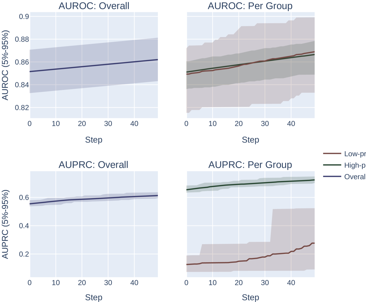
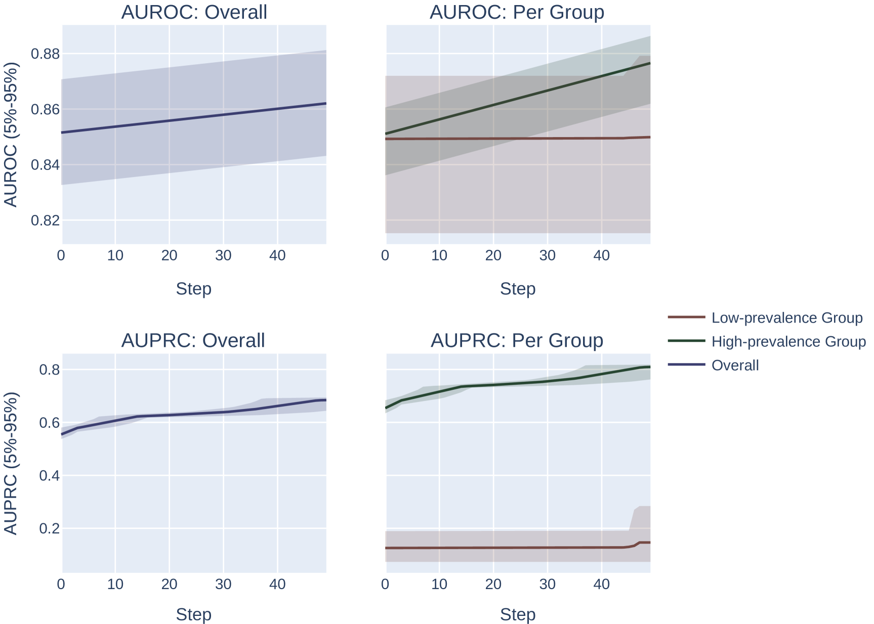
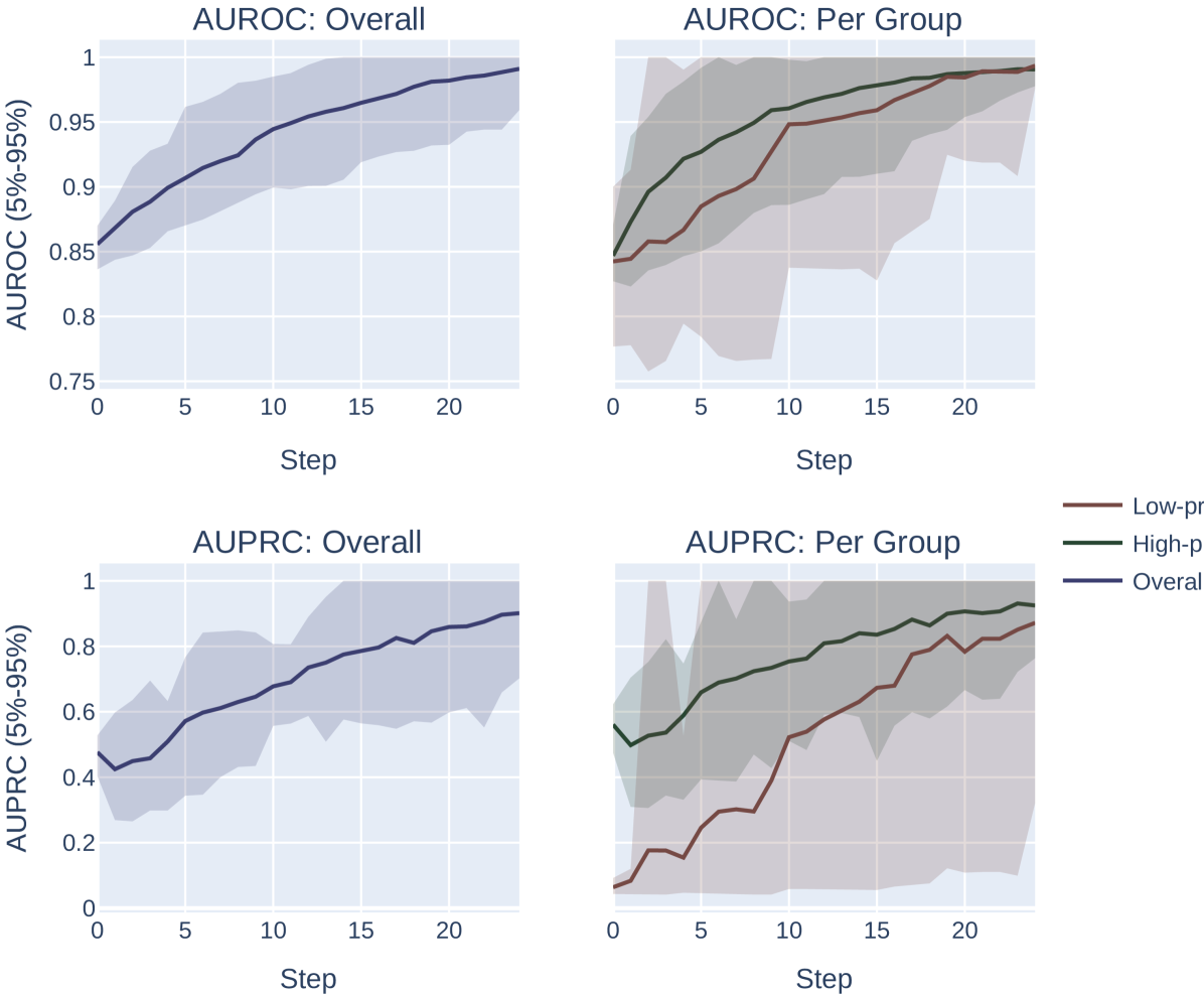
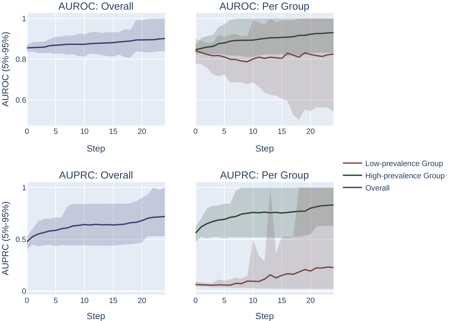
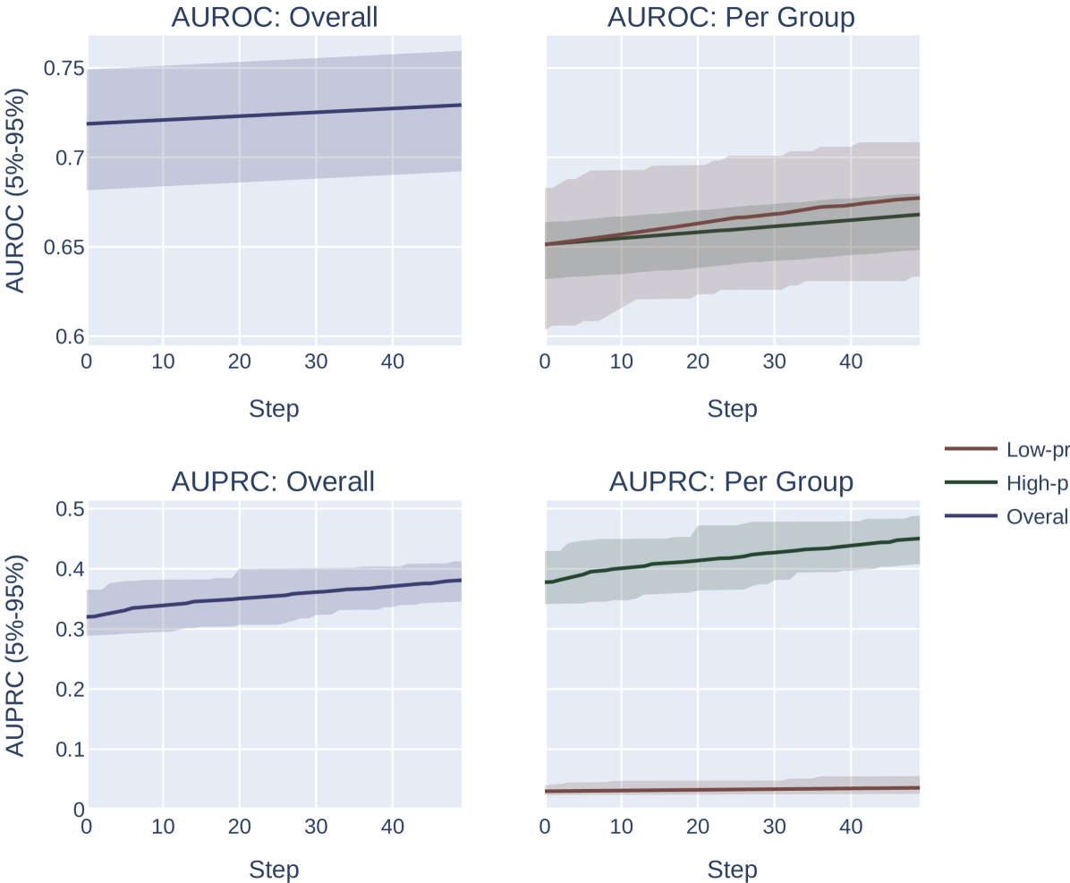
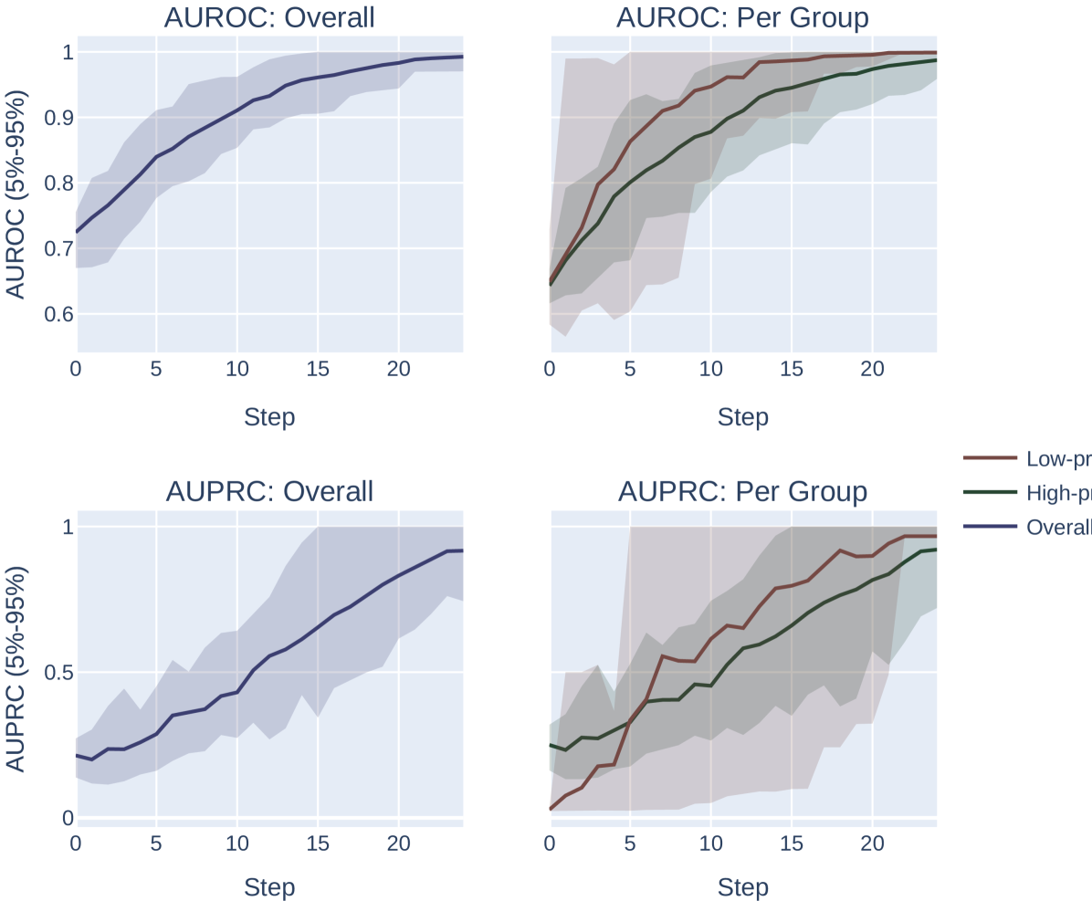
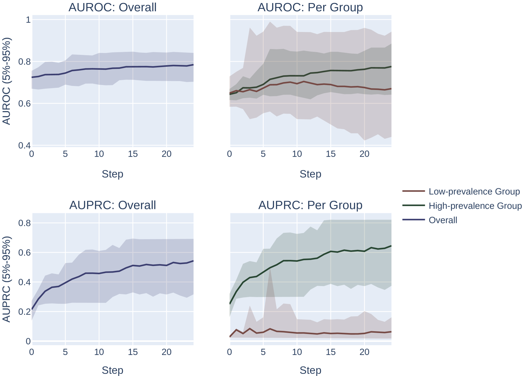
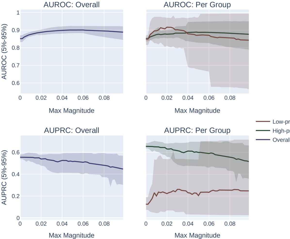
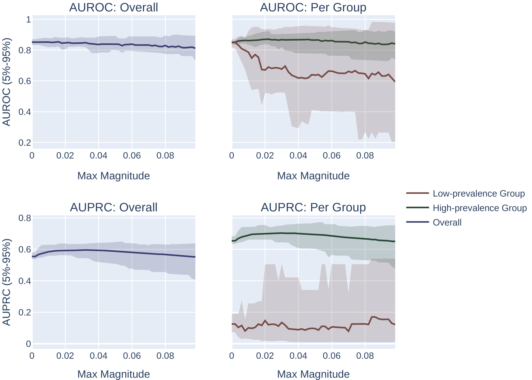
Appendix G Additional Details on Real World Experiments

G.1 Dataset Details

We use the following four datasets. In all datasets, we use sex and race as protected attributes.

• adult (Asuncion & Newman, 2007): The UCI Adult dataset, where the goal is to predict whether an individual’s income is $>\$50k$.

• compas (Angwin et al., 2022): The task to predict two-year recidivism. We only select samples belonging to “African-American” and “Caucasian”, leading to a binary race variable.

• lsac (Wightman, 1998): The task is to predict whether a law school applicant will pass the bar. We only select samples belonging to White and Black applicants.

• mimic (Johnson et al., 2016): We use the in-hospital mortality task proposed by Harutyunyan et al. (2019), where the goal is to predict whether a patient will die in the ICU given labs and vitals from the first 48 hours of their hospital stay. We only select samples belonging to White and Black patients.

In each dataset, we balance the groups by subsampling the majority group. We then split each dataset into 50% training, 25% validation, 25% test sets, stratified by the group. Dataset statistics can be found in Table 1.

Table 1: Dataset statistics for the four binary classification datasets used in this study. Note that $n$ refers to the number of samples after balancing by the corresponding attribute.

Dataset	Attribute	$𝐧$	# Features	Prevalence (Higher)	Prevalence (Lower)
adult	Sex	20,394	12	30.1%	10.7%
adult	Race	6,248	12	24.6%	12.2%
compas	Sex	2,438	6	52.0%	39.4%
compas	Race	4,908	6	55.4%	42.3%
lsac	Sex	15,906	8	96.0%	95.0%
lsac	Race	2,396	8	96.5%	77.2%
mimic	Sex	15,632	49	12.5%	11.9%
mimic	Race	4,030	49	13.9%	9.3%

G.2 Hyperparameter Grid

We use the following hyperparameter grid for our experiments:

• max depth: {1, 2, …, 9}

• learning rate: [0,01, 0.3]

• number of estimators: [50, 1000]

• min child weight: {1, 2, …, 9}

• use protected attribute as input feature: {yes, no}

• group weight of higher prevalence group: {1, 2, 3, 4, 5, 10, 15, 20, 25, 50}

G.3 Additional Results

Figure 7: Spearman’s $\rho$ between the test-set signed AUROC gap versus the validation set overall AUPRC, and the AUROC gap versus the overall AUROC. Numbers in parentheses are the prevalence ratios between the two groups for the particular attribute, and datasets are sorted by this quantity. Error bars are 95% confidence intervals from five different random data splits.

Figure 8: Correlation between the prevalence ratio, and the difference between the Spearman’s $\rho$ of the AUROC gap versus AUROC and the AUROC gap versus AUPRC. Each point represents a dataset and attribute combination. This correlation itself has a Spearman’s $\rho$ of $0.714$ (p = 0.047).

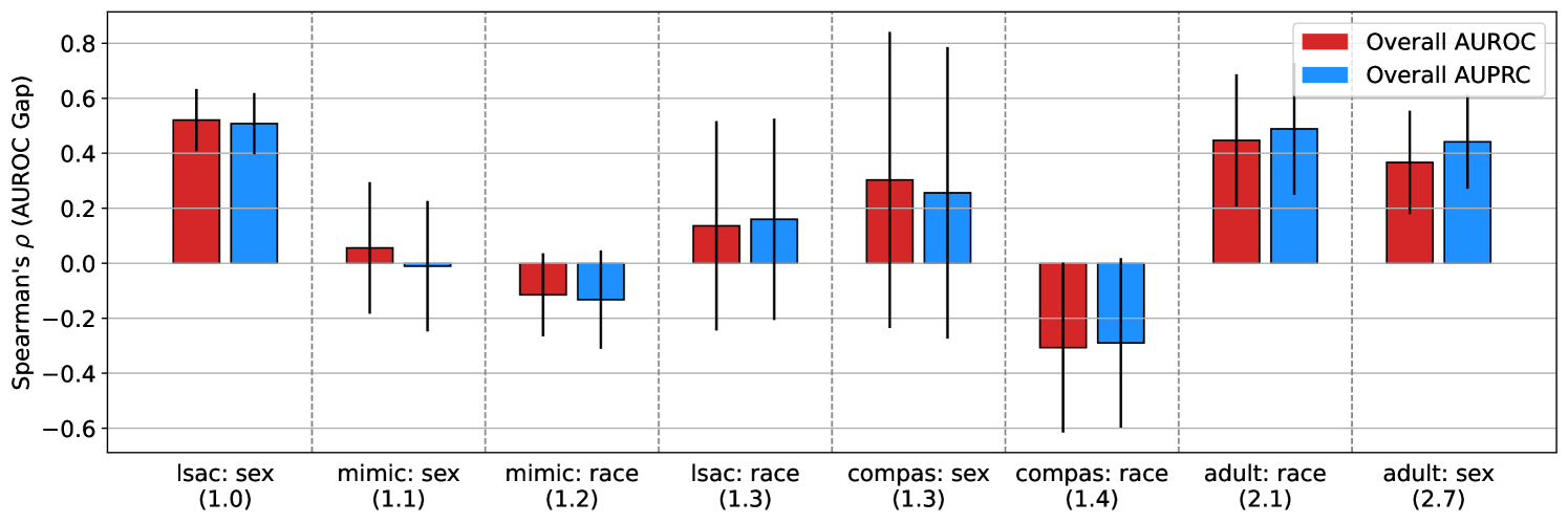
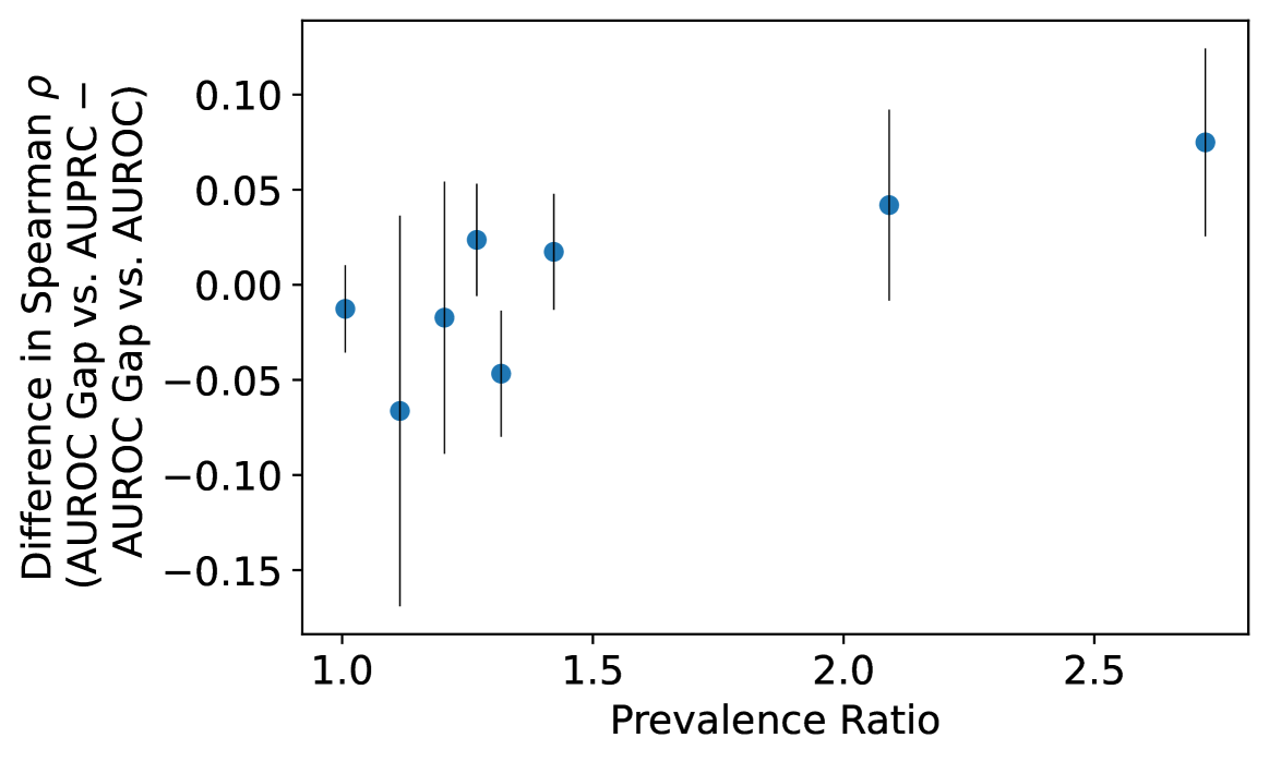
Appendix H Literature Review Methodology

H.1 Paper Acquisition

The initial phase of our comprehensive literature search involved the acquisition of datasets from both the Arxiv repository and NeurIPS conference proceedings. Utilizing the RedPajama dataset available through Hugging Face for Arxiv papers, and a custom scraper for NeurIPS papers, we specifically targeted these sources for our literature review. The Arxiv dataset, approximately 93.8 GB in size, encompassed over 1.5 million texts in JSONL format. For NeurIPS, we developed a script to scrape conference papers from 1987 to 2019 (9680 texts), aiming to enrich our search.

H.2 Keyword-Driven Filtering Process

1. Keyword List Development: We developed two distinct keyword lists to systematically identify papers relevant to our research on AUROC (Area Under the Receiver Operating Characteristic) and AUPRC (Area Under the Precision-Recall Curve) in our initial screening phase. The keyword lists can be accessed here for AUPRC and here for AUROC.

2. Automated Script-Based Search: Python scripts were employed to traverse the Arxiv and NeurIPS datasets. These scripts detected occurrences of our predefined keywords, allowing efficient parsing of a vast number of texts from both sources.

3. Dual Mention Selection Criterion: We focused on papers discussing both AUROC and AUPRC. This criterion ensured the relevance of the papers to our research question. Through this process, we narrowed the pool from 16,022 texts (containing either set of keywords) to 8,244 texts mentioning both in the Arxiv dataset. In the NeurIPS dataset, out of 9,680 texts reviewed, 78 were found to contain keywords from AUPRC and AUROC.

H.3 AI-Assisted Screening and Refinement

1. Preliminary Analysis with GPT-3.5: We utilized OpenAI’s GPT-3.5 model for an initial round of AI-assisted analysis for the arXiv dataset. This model identified and extracted papers making explicit claims regarding the comparative effectiveness of AUPRC over AUROC in scenarios of class imbalance, reducing our dataset from Arxiv to 2,728 papers.

2. Further Refinement Using GPT-4.0 Turbo: To refine our dataset further, we employed the GPT-4.0 Turbo model. Out of the 2,728 papers scrutinized from Arxiv using this model, 201 were found to be relevant. For NeurIPS, our focused search with GPT-4 resulted in identifying 2 papers of particular relevance to our thesis from the initial set that contained keywords related to both AUPRC and AUROC.

H.4 Manual Review

• Shared Document for Collaborative Analysis: We compiled all pertinent papers, along with their respective Arxiv IDs and the claims identified by GPT-4.0 Turbo, into a shared Google document for team review. Claims made in papers were found manually, and the specific quote of the claim they made was highlighted along with whether or not they had a citation for this claim.

H.4.1 Final Papers

After manual review, we identified 128 papers that make or reference some version of the claim that “AUPRC is better than AUROC in cases of class imbalance.” (Cook & Ramadas, 2020; Leisman, 2018; Yang et al., 2015; Gaudreault et al., 2021; Albora & Zaccaria, 2022; Lim & van der Schaar, 2018; Liu et al., 2023; Randl et al., 2023; Tusfiqur et al., 2022; Piermarini et al., 2023; Zhang & Bondell, 2018; Weiss & Tonella, 2021; Afanasiev et al., 2021; Li et al., 2022; Torfi et al., 2022; Wu et al., 2020; Miao & Zhu, 2022; Navarro et al., 2022; Cho et al., 2021; Wagner et al., 2023; Isupova et al., 2017; Sarvari et al., 2021; Hiri et al., 2022; Herbach, 2021; Si & Roberts, 2021; Narayanan et al., 2022; Li et al., 2020; Lee et al., 2013; Rayhan et al., 2017; Kyono et al., 2018; Adler, 2021; Seo et al., 2021; Hong et al., 2019; Hagedoorn & Spanakis, 2017; Yang et al., 2022a; Babaei et al., 2021; Garcin & Stéphan, 2021; Mehboudi et al., 2022; Yang et al., 2022b; Shen & Kursun, 2021; Muthukrishna et al., 2019; Deng et al., 2023; Yang, 2021; Harer et al., 2018; Meister et al., 2022; Skarding et al., 2021; Alvarez et al., 2022; Zou et al., 2022; Mangolin et al., 2022; Mosteiro et al., 2021; Hashemi et al., 2018; Lee et al., 2020; Zavrtanik et al., 2021; Showalter & Wu, 2019; Cranmer & Desmarais, 2016; Bryan & Moriano, 2023; Zhang et al., 2017; Domingues et al., 2020; Markdahl et al., 2017; Fu et al., 2021; Pang et al., 2023; Rezvani et al., 2021; Ozyegen et al., 2022; Prapas et al., 2023; Rayhan et al., 2020; Thambawita et al., 2020; Shukla & Marlin, 2019; Blevins et al., 2021; Vijayan et al., 2017; Budka et al., 2021; Hsu et al., 2020; Smith et al., 2023; Choi et al., 2018; Ju et al., 2018; Pashchenko et al., 2018; Chu et al., 2018; Silva et al., 2022; Bach Nguyen et al., 2022; Deshwar et al., 2015; Brophy & Lowd, 2020; Mayaki & Riveill, 2022; Mongia et al., 2021; Tiulpin et al., 2019; Romero et al., 2022; Rubin et al., 2012; Schwarz et al., 2021; Lyu et al., 2021; Lopez-Martinez et al., 2022; Ahmed & Courville, 2020; Gong et al., 2021; Zhang et al., 2021; Shukla & Marlin, 2018; Lund et al., 2019; Ma et al., 2022; Ruff et al., 2021; Lei Ba et al., 2015; Chakraborty et al., 2023; Rajabi & He, 2021; Newby et al., 2022; Axelrod & Gomez-Bombarelli, 2023; Kim et al., 2022; Ando & Huang, 2017; Stolman et al., 2022; Mosquera et al., 2022; Kulkarni et al., 2021; Won et al., 2019; Stephenson et al., 2022; Srivastava et al., 2019; Moor et al., 2019; Danesh Pazho et al., 2023; Kiran et al., 2018; Steinbuss & Böhm, 2021; Ma et al., 2020; Karadzhov et al., 2022; Ding et al., 2018; Mousavian et al., 2016; Rayhan et al., 2017; Vens et al., 2008; Rohani & Eslahchi, 2019; López et al., 2013; Sahiner et al., 2017; Rao et al., 2022; Hibshman & Weninger, 2023; Ntroumpogiannis et al., 2023; Weiss & Tonella, 2023; Hall et al., 2023; Goyal & Khiari, 2020; Boyd et al., 2013).

All papers identified, manual screening results, and extracted quotes can be found here: https://docs.google.com/spreadsheets/d/1NjDpwoj_8EkIwtGZzwM6w2nbst-LlGJPAqUcVINmPEk/edit?usp=sharing.

Claim	References	Commentary
Precision-recall curves or other associated metrics may more appropriately reflect deployment objectives than the receiver operating characteristic.	(Cook & Ramadas, 2020; Leisman, 2018; Yang et al., 2015; Muthukrishna et al., 2019; Deng et al., 2023; Harer et al., 2018; Ahmed & Courville, 2020)	While this claim is true, the informativeness of the PR curve for target deployment metrics is not sufficient to conclude that the AUPRC is superior to the AUROC in all cases of class imbalance. Despite this, it is often taken to assert this more general claim without caveat.
AUPRC does not depend on the number of true-negatives, so will be less optimistic than the AUROC	(Leisman, 2018; Kyono et al., 2018; Adler, 2021; Meister et al., 2022; Mosteiro et al., 2021; Showalter & Wu, 2019; Cranmer & Desmarais, 2016; Domingues et al., 2020; Rezvani et al., 2021; Hsu et al., 2020; Ju et al., 2018; Pashchenko et al., 2018; Romero et al., 2022; Vens et al., 2008)	As shown in Theorem 1, AUROC and AUPRC can both be naturally expressed as a function of the expectation of the model’s false positive rate. More generally, lack of dependence on one quadrant among the mutually dependent four quadrants of a confusion matrix is not an informative property for the AUROC and AUPRC metrics.
AUPRC will often be significantly lower, farther from optimality, and/or will grow more non-linearly as model performance improves than AUROC for low-prevalence tasks	(Leisman, 2018; Yang et al., 2015; Mehboudi et al., 2022; Cranmer & Desmarais, 2016)	Metric utility for model comparison depends on how appropriately it prioritizes model improvements, and is therefore less about the raw magnitude of the metric and more about the situations in which the order of a set of models will differ under one metric vs. another. One could easily make AUROC yield smaller values or grow more quickly near optimality by simply exponentiating it, but this would not yield a better metric.
AUPRC depends on prevalence, which is a desirable property	(Navarro et al., 2022)	This statement is too vague to be formally evaluated; whether or not this dependence on prevalence is desirable depends on the context. For model comparison in general, we argue it is not desirable in this form as it induces the biases inhere in AUPRC previously discussed.
AUPRC better captures differentiating a positive sample with high score from a “hard” negative sample (“hard” meaning one also with high score)	(Kiran et al., 2018)	While this claim is true by Theorem 2, it is not clear why this would be desired in general; this implicitly favors comparing “hard” negatives against “easy” positives as opposed to “easy” negatives against “hard” positives.
AUROC is otherwise “optimistic” in low-prevalence settings	(Cook & Ramadas, 2020; Afanasiev et al., 2021; Wu et al., 2020; Miao & Zhu, 2022; Cho et al., 2021; Hagedoorn & Spanakis, 2017; Yang et al., 2022a; Mangolin et al., 2022; Silva et al., 2022; Lyu et al., 2021; Ahmed & Courville, 2020; Zhang et al., 2021; Lund et al., 2019; Ruff et al., 2021; Chakraborty et al., 2023; Rajabi & He, 2021; Ando & Huang, 2017; Kulkarni et al., 2021; Karadzhov et al., 2022; Hibshman & Weninger, 2023)	This claim is underspecified, and un-true. AUROC always means the same thing, probabilistically, and that meaning independent from class imbalance.
AUPRC focues more on the positive (minority) class	(Tusfiqur et al., 2022; Wu et al., 2020; Si & Roberts, 2021; Narayanan et al., 2022; Babaei et al., 2021; Garcin & Stéphan, 2021; Deng et al., 2023; Alvarez et al., 2022; Mosteiro et al., 2021; Showalter & Wu, 2019; Pang et al., 2023; Ozyegen et al., 2022; Danesh Pazho et al., 2023; Kiran et al., 2018; López et al., 2013; Rao et al., 2022; Ntroumpogiannis et al., 2023)	This is unfounded; both AUROC and AUPRC are weighted expectations over the model’s false positive rate—AUPRC cares more about samples in regions of low firing rate, not explicitly about positive or minority samples.
AUROC can not appropriately detect models with poor recall	(Navarro et al., 2022)	This claim is unfounded; the AUROC clearly depends on the model’s recall. Besides, if recall is the measure of interest, then that should be measured explicitly.

Table 2: Various arguments and our responses to them present for this claim in the literature.

Claim	References	Valid?	Commentary
Precision-recall curves or other associated metrics may more appropriately reflect deployment objectives than the receiver operating characteristic.	(Cook & Ramadas, 2020; Leisman, 2018; Saito & Rehmsmeier, 2015; Yuan et al., 2015; Bleakley et al., 2007; Ozenne et al., 2015; Rosenberg, 2022; Zhou et al., 2020; Lichtnwalter & Chawla, 2012; Yang et al., 2015)	✓	While this claim is true, the informativeness of the PR curve for target deployment metrics is insufficient to conclude that the AUPRC is superior to the AUROC in all cases of class imbalance. Despite this, it is often taken to assert this more general claim without caveat.
AUPRC does not depend on the number of true negatives, so will be less optimistic than the AUROC	(Leisman, 2018; Goadrich et al., 2006; Cranmer & Desmarais, 2016)		As shown in Theorem 1, AUROC and AUPRC can both be naturally expressed as a function of the expectation of the model’s false positive rate. More generally, the lack of dependence on one quadrant among the mutually dependent four quadrants of a confusion matrix is not an informative property for the AUROC and AUPRC metrics.
AUPRC will often be significantly lower, farther from optimality, and/or will grow more non-linearly as model performance improves than AUROC for low-prevalence tasks	(Leisman, 2018; Yuan et al., 2015; Goadrich et al., 2006; Mazzanti, 2023; Rosenberg, 2022; Zhou et al., 2020; Lichtnwalter & Chawla, 2012; Yang et al., 2015; Cranmer & Desmarais, 2016)	✓	Metric utility for model comparison depends on how appropriately it prioritizes model improvements. Therefore, it is less about the raw magnitude of the metric and more about the situations in which the order of a set of models will differ under one metric vs. another. One could easily make AUROC yield smaller values or grow more quickly near optimality by simply exponentiating it, but this would not yield a better metric.
AUPRC depends on prevalence, which is a desirable property	(Saito & Rehmsmeier, 2015; Goadrich et al., 2006; Yuan et al., 2015)		This statement is too vague to be formally evaluated; whether or not this dependence on prevalence is desirable depends on the context. For model comparison in general, we argue it is not desirable in this form as it induces the biases in AUPRC previously discussed.
AUPRC better captures differentiating a positive sample with high score from a “hard” negative sample (“hard” meaning one also with high score)	(Rosenberg, 2022)	✓	While this claim is true by Theorem 2, it is not clear why this would be desired in general; this implicitly favors comparing “hard” negatives against “easy” positives as opposed to “easy” negatives against “hard” positives.

Table 3: Various arguments and our responses to them present for this claim in the literature.

H.5 Code Availability

All code pertaining to the literature review search can be found in the following GitHub repository: https://anonymous.4open.science/r/arxiv_neurips_search-3127/README.md

References

- Adler (2021) Adler, A. Using machine learning techniques to identify key risk factors for diabetes and undiagnosed diabetes, 2021.
- Afanasiev et al. (2021) Afanasiev, S., Smirnova, A., and Kotereva, D. Itsy bitsy spidernet: Fully connected residual network for fraud detection, 2021.
- Ahmed & Courville (2020) Ahmed, F. and Courville, A. Detecting semantic anomalies. Proceedings of the AAAI Conference on Artificial Intelligence, 34(04):3154–3162, Apr. 2020. doi: 10.1609/aaai.v34i04.5712. URL https://ojs.aaai.org/index.php/AAAI/article/view/5712.
- Albora & Zaccaria (2022) Albora, G. and Zaccaria, A. Machine learning to assess relatedness: the advantage of using firm-level data. Complexity, 2022, 2022.
- Alvarez et al. (2022) Alvarez, M., Verdier, J.-C., Nkashama, D. K., Frappier, M., Tardif, P.-M., and Kabanza, F. A revealing large-scale evaluation of unsupervised anomaly detection algorithms, 2022.
- Ando & Huang (2017) Ando, S. and Huang, C. Y. Deep over-sampling framework for classifying imbalanced data. In Machine Learning and Knowledge Discovery in Databases: European Conference, ECML PKDD 2017, Skopje, Macedonia, September 18–22, 2017, Proceedings, Part I 10, pp. 770–785. Springer, 2017.
- Angwin et al. (2022) Angwin, J., Larson, J., Mattu, S., and Kirchner, L. Machine bias. In Ethics of data and analytics, pp. 254–264. Auerbach Publications, 2022.
- Asuncion & Newman (2007) Asuncion, A. and Newman, D. Uci machine learning repository, 2007.
- Axelrod & Gomez-Bombarelli (2023) Axelrod, S. and Gomez-Bombarelli, R. Molecular machine learning with conformer ensembles. Machine Learning: Science and Technology, 4(3):035025, 2023.
- Babaei et al. (2021) Babaei, K., Chen, Z. Y., and Maul, T. Aegr: a simple approach to gradient reversal in autoencoders for network anomaly detection. Soft Computing, 25(24):15269–15280, 2021.
- Bach Nguyen et al. (2022) Bach Nguyen, V., Ghosh Dastidar, K., Granitzer, M., and Siblini, W. The importance of future information in credit card fraud detection. In Camps-Valls, G., Ruiz, F. J. R., and Valera, I. (eds.), Proceedings of The 25th International Conference on Artificial Intelligence and Statistics, volume 151 of Proceedings of Machine Learning Research, pp. 10067–10077. PMLR, 28–30 Mar 2022. URL https://proceedings.mlr.press/v151/bach-nguyen22a.html.
- Bergstra & Bengio (2012) Bergstra, J. and Bengio, Y. Random search for hyper-parameter optimization. Journal of machine learning research, 13(2), 2012.
- Bleakley et al. (2007) Bleakley, K., Biau, G., and Vert, J.-P. Supervised reconstruction of biological networks with local models. Bioinformatics, 23(13):i57–i65, 2007.
- Blevins et al. (2021) Blevins, D., Moriano, P., Bridges, R., Verma, M., Iannacone, M., and Hollifield, S. Time-based can intrusion detection benchmark. In Workshop on Automotive and Autonomous Vehicle Security (AutoSec), 2021.
- Boyd et al. (2013) Boyd, K., Eng, K. H., and Page, C. D. Area under the precision-recall curve: point estimates and confidence intervals. In Machine Learning and Knowledge Discovery in Databases: European Conference, ECML PKDD 2013, Prague, Czech Republic, September 23-27, 2013, Proceedings, Part III 13, pp. 451–466. Springer, 2013.
- Branco et al. (2016) Branco, P., Torgo, L., and Ribeiro, R. P. A survey of predictive modeling on imbalanced domains. ACM computing surveys (CSUR), 49(2):1–50, 2016.
- Brophy & Lowd (2020) Brophy, J. and Lowd, D. Eggs: A flexible approach to relational modeling of social network spam, 2020.
- Bryan & Moriano (2023) Bryan, J. and Moriano, P. Graph-based machine learning improves just-in-time defect prediction. Plos one, 18(4):e0284077, 2023.
- Budka et al. (2021) Budka, M., Ashraf, A. W. U., Bennett, M., Neville, S., and Mackrill, A. Deep multilabel cnn for forensic footwear impression descriptor identification. Applied Soft Computing, 109:107496, 2021.
- Burez & Van den Poel (2009) Burez, J. and Van den Poel, D. Handling class imbalance in customer churn prediction. Expert Systems with Applications, 36(3, Part 1):4626–4636, 2009. ISSN 0957-4174. doi: https://doi.org/10.1016/j.eswa.2008.05.027. URL https://www.sciencedirect.com/science/article/pii/S0957417408002121.
- Chakraborty et al. (2023) Chakraborty, N., Hasan, A., Liu, S., Ji, T., Liang, W., McPherson, D. L., and Driggs-Campbell, K. Structural attention-based recurrent variational autoencoder for highway vehicle anomaly detection. In Proceedings of the 2023 International Conference on Autonomous Agents and Multiagent Systems, AAMAS ’23, pp. 1125–1134, Richland, SC, 2023. International Foundation for Autonomous Agents and Multiagent Systems. ISBN 9781450394321.
- Chen & Guestrin (2016) Chen, T. and Guestrin, C. Xgboost: A scalable tree boosting system. In Proceedings of the 22nd acm sigkdd international conference on knowledge discovery and data mining, pp. 785–794, 2016.
- Cho et al. (2021) Cho, B. Y., Hermans, T., and Kuntz, A. Planning sensing sequences for subsurface 3d tumor mapping. In 2021 International Symposium on Medical Robotics (ISMR), pp. 1–7. IEEE, 2021.
- Choi et al. (2018) Choi, E., Xiao, C., Stewart, W. F., and Sun, J. Mime: Multilevel medical embedding of electronic health records for predictive healthcare. In Proceedings of the 32nd International Conference on Neural Information Processing Systems, NIPS’18, pp. 4552–4562, Red Hook, NY, USA, 2018. Curran Associates Inc.
- Chu et al. (2018) Chu, X., Lin, Y., Gao, J., Wang, J., Wang, Y., and Wang, L. Multi-label robust factorization autoencoder and its application in predicting drug-drug interactions, 2018.
- Cook & Ramadas (2020) Cook, J. and Ramadas, V. When to consult precision-recall curves. The Stata Journal, 20(1):131–148, 2020.
- Cranmer & Desmarais (2016) Cranmer, S. J. and Desmarais, B. A. What can we learn from predictive modeling?, 2016.
- Czakon (2022) Czakon, J. F1 Score vs ROC AUC vs Accuracy vs PR AUC: Which Evaluation Metric Should You Choose?, July 2022. URL https://neptune.ai/blog/f1-score-accuracy-roc-auc-pr-auc.
- Danesh Pazho et al. (2023) Danesh Pazho, A., Alinezhad Noghre, G., Rahimi Ardabili, B., Neff, C., and Tabkhi, H. CHAD: Charlotte Anomaly Dataset, pp. 50–66. Springer Nature Switzerland, 2023. ISBN 9783031314353. doi: 10.1007/978-3-031-31435-3˙4. URL http://dx.doi.org/10.1007/978-3-031-31435-3_4.
- Davis & Goadrich (2006) Davis, J. and Goadrich, M. The relationship between precision-recall and roc curves. In Proceedings of the 23rd International Conference on Machine Learning, ICML ’06, pp. 233–240, New York, NY, USA, 2006. Association for Computing Machinery. ISBN 1595933832. doi: 10.1145/1143844.1143874. URL https://doi.org/10.1145/1143844.1143874.
- Deng et al. (2023) Deng, J., Yang, Z., Wang, H., Ojima, I., Samaras, D., and Wang, F. Unraveling key elements underlying molecular property prediction: A systematic study, 2023.
- Deshwar et al. (2015) Deshwar, A. G., Vembu, S., Yung, C. K., Jang, G. H., Stein, L., and Morris, Q. Reconstructing subclonal composition and evolution from whole genome sequencing of tumors, 2015.
- Ding et al. (2018) Ding, D. Y., Simpson, C., Pfohl, S., Kale, D. C., Jung, K., and Shah, N. H. The effectiveness of multitask learning for phenotyping with electronic health records data. In BIOCOMPUTING 2019: Proceedings of the Pacific Symposium, pp. 18–29. World Scientific, 2018.
- Domingues et al. (2020) Domingues, R., Michiardi, P., Barlet, J., and Filippone, M. A comparative evaluation of novelty detection algorithms for discrete sequences. Artificial Intelligence Review, 53:3787–3812, 2020.
- Dressel & Farid (2018) Dressel, J. and Farid, H. The accuracy, fairness, and limits of predicting recidivism. Science advances, 4(1):eaao5580, 2018.
- Ezzat et al. (2017) Ezzat, A., Zhao, P., Wu, M., Li, X.-L., and Kwoh, C.-K. Drug-target interaction prediction with graph regularized matrix factorization. IEEE/ACM Transactions on Computational Biology and Bioinformatics, 14(3):646–656, 2017. doi: 10.1109/TCBB.2016.2530062.
- Fabris et al. (2022) Fabris, A., Messina, S., Silvello, G., and Susto, G. A. Algorithmic fairness datasets: the story so far. Data Mining and Knowledge Discovery, 36(6):2074–2152, 2022.
- Flach & Kull (2015) Flach, P. and Kull, M. Precision-recall-gain curves: Pr analysis done right. Advances in neural information processing systems, 28, 2015.
- Flach et al. (2011) Flach, P., Hernández-Orallo, J., and Ferri, C. A coherent interpretation of auc as a measure of aggregated classification performance. In Proceedings of the 28th International Conference on International Conference on Machine Learning, ICML’11, pp. 657–664, Madison, WI, USA, 2011. Omnipress. ISBN 9781450306195.
- Fu et al. (2021) Fu, Y., Wu, X.-B., Yang, Q., Brown, A. G., Feng, X., Ma, Q., and Li, S. Finding quasars behind the galactic plane. i. candidate selections with transfer learning. The Astrophysical Journal Supplement Series, 254(1):6, 2021.
- Garcin & Stéphan (2021) Garcin, M. and Stéphan, S. Credit scoring using neural networks and sure posterior probability calibration, 2021.
- Gaudreault et al. (2021) Gaudreault, J.-G., Branco, P., and Gama, J. An analysis of performance metrics for imbalanced classification. In International Conference on Discovery Science, pp. 67–77. Springer, 2021.
- Goadrich et al. (2006) Goadrich, M., Oliphant, L., and Shavlik, J. Gleaner: Creating ensembles of first-order clauses to improve recall-precision curves. Machine Learning, 64:231–261, 2006.
- Gong et al. (2021) Gong, H., Valido, A., Ingram, K. M., Fanti, G., Bhat, S., and Espelage, D. L. Abusive language detection in heterogeneous contexts: Dataset collection and the role of supervised attention. In Proceedings of the AAAI Conference on Artificial Intelligence, volume 35(17), pp. 14804–14812, 2021.
- Goyal & Khiari (2020) Goyal, A. and Khiari, J. Diversity-aware weighted majority vote classifier for imbalanced data. In 2020 International Joint Conference on Neural Networks (IJCNN), pp. 1–8, 2020. doi: 10.1109/IJCNN48605.2020.9207261.
- Hagedoorn & Spanakis (2017) Hagedoorn, T. R. and Spanakis, G. Massive open online courses temporal profiling for dropout prediction. In 2017 IEEE 29th International Conference on Tools with Artificial Intelligence (ICTAI), pp. 231–238. IEEE, 2017.
- Hall et al. (2023) Hall, M., Chern, B., Gustafson, L., Ventura, D., Kulkarni, H., Ross, C., and Usunier, N. Towards reliable assessments of demographic disparities in multi-label image classifiers, 2023.
- Harer et al. (2018) Harer, J. A., Kim, L. Y., Russell, R. L., Ozdemir, O., Kosta, L. R., Rangamani, A., Hamilton, L. H., Centeno, G. I., Key, J. R., Ellingwood, P. M., Antelman, E., Mackay, A., McConley, M. W., Opper, J. M., Chin, P., and Lazovich, T. Automated software vulnerability detection with machine learning, 2018.
- Harutyunyan et al. (2019) Harutyunyan, H., Khachatrian, H., Kale, D. C., Ver Steeg, G., and Galstyan, A. Multitask learning and benchmarking with clinical time series data. Scientific data, 6(1):96, 2019.
- Hashemi et al. (2018) Hashemi, S. R., Salehi, S. S. M., Erdogmus, D., Prabhu, S. P., Warfield, S. K., and Gholipour, A. Asymmetric loss functions and deep densely-connected networks for highly-imbalanced medical image segmentation: Application to multiple sclerosis lesion detection. IEEE Access, 7:1721–1735, 2018.
- He & Garcia (2009) He, H. and Garcia, E. A. Learning from imbalanced data. IEEE Transactions on Knowledge and Data Engineering, 21(9):1263–1284, 2009. doi: 10.1109/TKDE.2008.239.
- Herbach (2021) Herbach, U. Gene regulatory network inference from single-cell data using a self-consistent proteomic field, 2021.
- Hibshman & Weninger (2023) Hibshman, J. I. and Weninger, T. Inherent limits on topology-based link prediction, 2023.
- Hicks et al. (2022) Hicks, S. A., Strümke, I., Thambawita, V., Hammou, M., Riegler, M. A., Halvorsen, P., and Parasa, S. On evaluation metrics for medical applications of artificial intelligence. Scientific reports, 12(1):5979, 2022.
- Hiri et al. (2022) Hiri, K. D., Hren, M., and Curk, T. Nlp-based classification of software tools for metagenomics sequencing data analysis into edam semantic annotation, 2022.
- Hong et al. (2019) Hong, S., Xiao, C., Hoang, T. N., Ma, T., Li, H., and Sun, J. Rdpd: Rich data helps poor data via imitation. In 28th International Joint Conference on Artificial Intelligence, IJCAI 2019, pp. 5895–5901. International Joint Conferences on Artificial Intelligence, 2019.
- Hsu et al. (2020) Hsu, C.-C., Karnwal, S., Mullainathan, S., Obermeyer, Z., and Tan, C. Characterizing the value of information in medical notes. In Cohn, T., He, Y., and Liu, Y. (eds.), Findings of the Association for Computational Linguistics: EMNLP 2020, pp. 2062–2072, Online, November 2020. Association for Computational Linguistics. doi: 10.18653/v1/2020.findings-emnlp.187. URL https://aclanthology.org/2020.findings-emnlp.187.
- Isupova et al. (2017) Isupova, O., Kuzin, D., and Mihaylova, L. Learning methods for dynamic topic modeling in automated behavior analysis. IEEE transactions on neural networks and learning systems, 29(9):3980–3993, 2017.
- Johnson et al. (2016) Johnson, A. E., Pollard, T. J., Shen, L., Lehman, L.-w. H., Feng, M., Ghassemi, M., Moody, B., Szolovits, P., Anthony Celi, L., and Mark, R. G. Mimic-iii, a freely accessible critical care database. Scientific data, 3(1):1–9, 2016.
- Ju et al. (2018) Ju, C., Li, J., Wasti, B., and Guo, S. Semisupervised learning on heterogeneous graphs and its applications to facebook news feed, 2018.
- Karadzhov et al. (2022) Karadzhov, G., Stafford, T., and Vlachos, A. What makes you change your mind? an empirical investigation in online group decision-making conversations, 2022.
- Kim et al. (2022) Kim, M., Kim, J., Yu, J., and Choi, J. K. Unsupervised deep one-class classification with adaptive threshold based on training dynamics. In 2022 IEEE International Conference on Data Mining Workshops (ICDMW), pp. 39–46, 2022. doi: 10.1109/ICDMW58026.2022.00014.
- Kiran et al. (2018) Kiran, B. R., Thomas, D. M., and Parakkal, R. An overview of deep learning based methods for unsupervised and semi-supervised anomaly detection in videos. Journal of Imaging, 4(2), 2018. ISSN 2313-433X. doi: 10.3390/jimaging4020036. URL https://www.mdpi.com/2313-433X/4/2/36.
- Krawczyk (2016) Krawczyk, B. Learning from imbalanced data: open challenges and future directions. Progress in Artificial Intelligence, 5(4):221–232, 2016.
- Kulkarni et al. (2021) Kulkarni, V., Gawali, M., and Kharat, A. Key technology considerations in developing and deploying machine learning models in clinical radiology practice. JMIR Med Inform, 9(9):e28776, Sep 2021. ISSN 2291-9694. doi: 10.2196/28776. URL https://medinform.jmir.org/2021/9/e28776.
- Kyono et al. (2018) Kyono, T., Gilbert, F. J., and van der Schaar, M. Mammo: A deep learning solution for facilitating radiologist-machine collaboration in breast cancer diagnosis, 2018.
- Lahoti et al. (2020) Lahoti, P., Beutel, A., Chen, J., Lee, K., Prost, F., Thain, N., Wang, X., and Chi, E. Fairness without demographics through adversarially reweighted learning. Advances in neural information processing systems, 33:728–740, 2020.
- LCT14558 (2017) LCT14558. Imbalanced data & why you should NOT use ROC curve, March 2017. URL https://kaggle.com/code/lct14558/imbalanced-data-why-you-should-not-use-roc-curve.
- Lee et al. (2013) Lee, C., Nick, B., Brandes, U., and Cunningham, P. Link prediction with social vector clocks. In Proceedings of the 19th ACM SIGKDD international conference on Knowledge discovery and data mining, pp. 784–792, 2013.
- Lee et al. (2020) Lee, I.-T., Marwah, M., and Arlitt, M. Attention-based self-supervised feature learning for security data, 2020.
- Lei Ba et al. (2015) Lei Ba, J., Swersky, K., Fidler, S., et al. Predicting deep zero-shot convolutional neural networks using textual descriptions. In Proceedings of the IEEE international conference on computer vision, pp. 4247–4255, 2015.
- Leisman (2018) Leisman, D. E. Rare events in the icu: an emerging challenge in classification and prediction. Critical care medicine, 46(3):418–424, 2018.
- Li et al. (2022) Li, Q., Zhang, Y., Qiu, D., He, Y., Cao, L., and Woodland, P. C. Improving confidence estimation on out-of-domain data for end-to-end speech recognition. In ICASSP 2022-2022 IEEE International Conference on Acoustics, Speech and Signal Processing (ICASSP), pp. 6537–6541. IEEE, 2022.
- Li et al. (2020) Li, X., Al-Zaidy, R., Zhang, A., Baral, S., Bao, L., and Giles, C. L. Automating document classification with distant supervision to increase the efficiency of systematic reviews, 2020.
- Lichtnwalter & Chawla (2012) Lichtnwalter, R. and Chawla, N. V. Link prediction: fair and effective evaluation. In 2012 IEEE/ACM International Conference on Advances in Social Networks Analysis and Mining, pp. 376–383. IEEE, 2012.
- Lim & van der Schaar (2018) Lim, B. and van der Schaar, M. Disease-atlas: Navigating disease trajectories using deep learning. In Machine Learning for Healthcare Conference, pp. 137–160. PMLR, 2018.
- Liu et al. (2023) Liu, Y., Yang, D., Wang, Y., Liu, J., Liu, J., Boukerche, A., Sun, P., and Song, L. Generalized video anomaly event detection: Systematic taxonomy and comparison of deep models, 2023.
- Lobo et al. (2008) Lobo, J. M., Jiménez-Valverde, A., and Real, R. Auc: a misleading measure of the performance of predictive distribution models. Global Ecology and Biogeography, 17(2):145–151, 2008. doi: https://doi.org/10.1111/j.1466-8238.2007.00358.x. URL https://onlinelibrary.wiley.com/doi/abs/10.1111/j.1466-8238.2007.00358.x.
- Lopez-Martinez et al. (2022) Lopez-Martinez, D., Yakubovich, A., Seneviratne, M., Lelkes, A. D., Tyagi, A., Kemp, J., Steinberg, E., Downing, N. L., Li, R. C., Morse, K. E., Shah, N. H., and Chen, M.-J. Instability in clinical risk stratification models using deep learning. In Parziale, A., Agrawal, M., Joshi, S., Chen, I. Y., Tang, S., Oala, L., and Subbaswamy, A. (eds.), Proceedings of the 2nd Machine Learning for Health symposium, volume 193 of Proceedings of Machine Learning Research, pp. 552–565. PMLR, 28 Nov 2022. URL https://proceedings.mlr.press/v193/lopez-martinez22a.html.
- Lund et al. (2019) Lund, J., Armstrong, P., Fearn, W., Cowley, S., Hales, E., and Seppi, K. Cross-referencing using fine-grained topic modeling. In Burstein, J., Doran, C., and Solorio, T. (eds.), Proceedings of the 2019 Conference of the North American Chapter of the Association for Computational Linguistics: Human Language Technologies, Volume 1 (Long and Short Papers), pp. 3978–3987, Minneapolis, Minnesota, June 2019. Association for Computational Linguistics. doi: 10.18653/v1/N19-1399. URL https://aclanthology.org/N19-1399.
- Lyu et al. (2021) Lyu, Y., Rajbahadur, G. K., Lin, D., Chen, B., and Jiang, Z. M. J. Towards a consistent interpretation of aiops models. ACM Trans. Softw. Eng. Methodol., 31(1), nov 2021. ISSN 1049-331X. doi: 10.1145/3488269. URL https://doi.org/10.1145/3488269.
- López et al. (2013) López, V., Fernández, A., García, S., Palade, V., and Herrera, F. An insight into classification with imbalanced data: Empirical results and current trends on using data intrinsic characteristics. Information Sciences, 250:113–141, 2013. ISSN 0020-0255. doi: https://doi.org/10.1016/j.ins.2013.07.007. URL https://www.sciencedirect.com/science/article/pii/S0020025513005124.
- Ma et al. (2020) Ma, L., Zhang, C., Wang, Y., Ruan, W., Wang, J., Tang, W., Ma, X., Gao, X., and Gao, J. Concare: Personalized clinical feature embedding via capturing the healthcare context. In Proceedings of the AAAI Conference on Artificial Intelligence, volume 34(01), pp. 833–840, 2020.
- Ma et al. (2022) Ma, X., Chu, X., Wang, Y., Yu, H., Ma, L., Tang, W., and Zhao, J. Medfact: Modeling medical feature correlations in patient health representation learning via feature clustering, 2022.
- Mangolin et al. (2022) Mangolin, R. B., Pereira, R. M., Britto Jr, A. S., Silla Jr, C. N., Feltrim, V. D., Bertolini, D., and Costa, Y. M. A multimodal approach for multi-label movie genre classification. Multimedia Tools and Applications, 81(14):19071–19096, 2022.
- Markdahl et al. (2017) Markdahl, J., Colombo, N., Thunberg, J., and Gonçalves, J. Experimental design trade-offs for gene regulatory network inference: An in silico study of the yeast saccharomyces cerevisiae cell cycle. In 2017 IEEE 56th Annual Conference on Decision and Control (CDC), pp. 423–428. IEEE, 2017.
- Mayaki & Riveill (2022) Mayaki, M. Z. A. and Riveill, M. Multiple inputs neural networks for fraud detection. In 2022 International Conference on Machine Learning, Control, and Robotics (MLCR), pp. 8–13, 2022. doi: 10.1109/MLCR57210.2022.00011.
- Mazzanti (2023) Mazzanti, S. Why you should stop using the ROC curve, September 2023. URL https://towardsdatascience.com/why-you-should-stop-using-the-roc-curve-a46a9adc728.
- Mehboudi et al. (2022) Mehboudi, A., Singhal, S., and Sreenivasan, S. V. Squeeze flow of micro-droplets: convolutional neural network with trainable and tunable refinement, 2022.
- Meister et al. (2022) Meister, J. A., Nguyen, K. A., and Luo, Z. Audio feature ranking for sound-based covid-19 patient detection. In EPIA Conference on Artificial Intelligence, pp. 146–158. Springer, 2022.
- Miao & Zhu (2022) Miao, J. and Zhu, W. Precision–recall curve (prc) classification trees. Evolutionary intelligence, 15(3):1545–1569, 2022.
- Mongia et al. (2021) Mongia, A., Saha, S. K., Chouzenoux, E., and Majumdar, A. A computational approach to aid clinicians in selecting anti-viral drugs for covid-19 trials. Scientific reports, 11(1):9047, 2021.
- Moor et al. (2019) Moor, M., Horn, M., Rieck, B., Roqueiro, D., and Borgwardt, K. Early recognition of sepsis with gaussian process temporal convolutional networks and dynamic time warping. In Doshi-Velez, F., Fackler, J., Jung, K., Kale, D., Ranganath, R., Wallace, B., and Wiens, J. (eds.), Proceedings of the 4th Machine Learning for Healthcare Conference, volume 106 of Proceedings of Machine Learning Research, pp. 2–26. PMLR, 09–10 Aug 2019. URL https://proceedings.mlr.press/v106/moor19a.html.
- Mosquera et al. (2022) Mosquera, C., Ferrer, L., Milone, D., Luna, D., and Ferrante, E. Impact of class imbalance on chest x-ray classifiers: towards better evaluation practices for discrimination and calibration performance, 2022.
- Mosteiro et al. (2021) Mosteiro, P., Rijcken, E., Zervanou, K., Kaymak, U., Scheepers, F., and Spruit, M. Machine learning for violence risk assessment using dutch clinical notes. Journal of Artificial Intelligence for Medical Sciences, 2(1-2):44–54, 2021.
- Mousavian et al. (2016) Mousavian, Z., Khakabimamaghani, S., Kavousi, K., and Masoudi-Nejad, A. Drug–target interaction prediction from pssm based evolutionary information. Journal of pharmacological and toxicological methods, 78:42–51, 2016.
- Muthukrishna et al. (2019) Muthukrishna, D., Narayan, G., Mandel, K. S., Biswas, R., and Hložek, R. Rapid: early classification of explosive transients using deep learning. Publications of the Astronomical Society of the Pacific, 131(1005):118002, 2019.
- Narayanan et al. (2022) Narayanan, S., Maple, C., and Hooper, M. A point process model for rare event detection, 2022.
- Navarro et al. (2022) Navarro, J. M., Huet, A., and Rossi, D. Human readable network troubleshooting based on anomaly detection and feature scoring. Computer Networks, 219:109447, 2022.
- Newby et al. (2022) Newby, E., Tejeda Zañudo, J. G., and Albert, R. Structure-based approach to identifying small sets of driver nodes in biological networks. Chaos: An Interdisciplinary Journal of Nonlinear Science, 32(6):063102, 06 2022. ISSN 1054-1500. doi: 10.1063/5.0080843. URL https://doi.org/10.1063/5.0080843.
- Ntroumpogiannis et al. (2023) Ntroumpogiannis, A., Giannoulis, M., Myrtakis, N., Christophides, V., Simon, E., and Tsamardinos, I. A meta-level analysis of online anomaly detectors. The VLDB Journal, pp. 1–42, 2023.
- Ozenne et al. (2015) Ozenne, B., Subtil, F., and Maucort-Boulch, D. The precision–recall curve overcame the optimism of the receiver operating characteristic curve in rare diseases. Journal of clinical epidemiology, 68(8):855–859, 2015.
- Ozyegen et al. (2022) Ozyegen, O., Kabe, D., and Cevik, M. Word-level text highlighting of medical texts for telehealth services. Artificial Intelligence in Medicine, 127:102284, 2022.
- Pang et al. (2023) Pang, G., Shen, C., Jin, H., and van den Hengel, A. Deep weakly-supervised anomaly detection. In Proceedings of the 29th ACM SIGKDD Conference on Knowledge Discovery and Data Mining, KDD ’23, pp. 1795–1807, New York, NY, USA, 2023. Association for Computing Machinery. ISBN 9798400701030. doi: 10.1145/3580305.3599302. URL https://doi.org/10.1145/3580305.3599302.
- Pashchenko et al. (2018) Pashchenko, I. N., Sokolovsky, K. V., and Gavras, P. Machine learning search for variable stars. Monthly Notices of the Royal Astronomical Society, 475(2):2326–2343, 2018.
- Pfohl et al. (2022) Pfohl, S., Xu, Y., Foryciarz, A., Ignatiadis, N., Genkins, J., and Shah, N. Net benefit, calibration, threshold selection, and training objectives for algorithmic fairness in healthcare. In Proceedings of the 2022 ACM Conference on Fairness, Accountability, and Transparency, pp. 1039–1052, 2022.
- Piermarini et al. (2023) Piermarini, D., Sudoso, A. M., and Piccialli, V. Predicting municipalities in financial distress: a machine learning approach enhanced by domain expertise, 2023.
- Prapas et al. (2023) Prapas, I., Ahuja, A., Kondylatos, S., Karasante, I., Panagiotou, E., Alonso, L., Davalas, C., Michail, D., Carvalhais, N., and Papoutsis, I. Deep learning for global wildfire forecasting, 2023.
- Provost & Fawcett (1997) Provost, F. and Fawcett, T. Analysis and visualization of classifier performance with nonuniform class and cost distributions. In Proceedings of AAAI-97 Workshop on AI Approaches to Fraud Detection & Risk Management, pp. 57–63, 1997.
- Rajabi & He (2021) Rajabi, F. and He, J. S. Click-through rate prediction using graph neural networks and online learning, 2021.
- Randl et al. (2023) Randl, K., Armengol, N. L., Mondrejevski, L., and Miliou, I. Early prediction of the risk of icu mortality with deep federated learning. In 2023 IEEE 36th International Symposium on Computer-Based Medical Systems (CBMS), pp. 706–711. IEEE, 2023.
- Rao et al. (2022) Rao, S. X., Lanfranchi, C., Zhang, S., Han, Z., Zhang, Z., Min, W., Cheng, M., Shan, Y., Zhao, Y., and Zhang, C. Modelling graph dynamics in fraud detection with ”attention”, 2022.
- Rayhan et al. (2017) Rayhan, F., Ahmed, S., Shatabda, S., Farid, D. M., Mousavian, Z., Dehzangi, A., and Rahman, M. S. idti-esboost: identification of drug target interaction using evolutionary and structural features with boosting. Scientific reports, 7(1):17731, 2017.
- Rayhan et al. (2020) Rayhan, F., Ahmed, S., Mousavian, Z., Farid, D. M., and Shatabda, S. Frnet-dti: Deep convolutional neural network for drug-target interaction prediction. Heliyon, 6(3), 2020.
- Rezvani et al. (2021) Rezvani, R., Kouchaki, S., Nilforooshan, R., Sharp, D. J., and Barnaghi, P. Semi-supervised learning for identifying the likelihood of agitation in people with dementia, 2021.
- Rohani & Eslahchi (2019) Rohani, N. and Eslahchi, C. Drug-drug interaction predicting by neural network using integrated similarity. Scientific reports, 9(1):13645, 2019.
- Romero et al. (2022) Romero, M., Ramírez, O., Finke, J., and Rocha, C. Feature extraction with spectral clustering for gene function prediction using hierarchical multi-label classification. Applied Network Science, 7(1):28, 2022.
- Rosenberg (2022) Rosenberg, D. Imbalanced Data? Stop Using ROC-AUC and Use AUPRC Instead, June 2022. URL https://towardsdatascience.com/imbalanced-data-stop-using-roc-auc-and-use-auprc-instead-46af4910a494.
- Rubin et al. (2012) Rubin, T. N., Chambers, A., Smyth, P., and Steyvers, M. Statistical topic models for multi-label document classification. Machine learning, 88:157–208, 2012.
- Ruff et al. (2021) Ruff, L., Kauffmann, J. R., Vandermeulen, R. A., Montavon, G., Samek, W., Kloft, M., Dietterich, T. G., and Müller, K.-R. A unifying review of deep and shallow anomaly detection. Proceedings of the IEEE, 109(5):756–795, 2021. doi: 10.1109/JPROC.2021.3052449.
- Sahiner et al. (2017) Sahiner, B., Chen, W., Pezeshk, A., and Petrick, N. Comparison of two classifiers when the data sets are imbalanced: the power of the area under the precision-recall curve as the figure of merit versus the area under the ROC curve. In Kupinski, M. A. and Nishikawa, R. M. (eds.), Medical Imaging 2017: Image Perception, Observer Performance, and Technology Assessment, volume 10136, pp. 101360G. International Society for Optics and Photonics, SPIE, 2017. doi: 10.1117/12.2254742. URL https://doi.org/10.1117/12.2254742.
- Saito & Rehmsmeier (2015) Saito, T. and Rehmsmeier, M. The precision-recall plot is more informative than the roc plot when evaluating binary classifiers on imbalanced datasets. PloS one, 10(3):e0118432, 2015.
- Sarvari et al. (2021) Sarvari, H., Domeniconi, C., Prenkaj, B., and Stilo, G. Unsupervised boosting-based autoencoder ensembles for outlier detection. In Pacific-Asia Conference on Knowledge Discovery and Data Mining, pp. 91–103. Springer, 2021.
- Schwarz et al. (2021) Schwarz, K., Allam, A., Perez Gonzalez, N. A., and Krauthammer, M. Attentionddi: Siamese attention-based deep learning method for drug–drug interaction predictions. BMC bioinformatics, 22(1):1–19, 2021.
- Seo et al. (2021) Seo, E., Hutchinson, R. A., Fu, X., Li, C., Hallman, T. A., Kilbride, J., and Robinson, W. D. Stateconet: Statistical ecology neural networks for species distribution modeling. In Proceedings of the AAAI Conference on Artificial Intelligence, volume 35, pp. 513–521, 2021.
- Shen & Kursun (2021) Shen, H. and Kursun, E. Label augmentation via time-based knowledge distillation for financial anomaly detection, 2021.
- Showalter & Wu (2019) Showalter, S. and Wu, Z. Minimizing the societal cost of credit card fraud with limited and imbalanced data, 2019.
- Shukla & Marlin (2019) Shukla, S. N. and Marlin, B. Interpolation-prediction networks for irregularly sampled time series. In International Conference on Learning Representations, 2019. URL https://openreview.net/forum?id=r1efr3C9Ym.
- Shukla & Marlin (2018) Shukla, S. N. and Marlin, B. M. Modeling irregularly sampled clinical time series, 2018.
- Si & Roberts (2021) Si, Y. and Roberts, K. Three-level hierarchical transformer networks for long-sequence and multiple clinical documents classification, 2021.
- Silva et al. (2022) Silva, M. C. R., Siqueira, F. A., Tarrega, J. P. M., Beinotti, J. V. P., Nunes, A. S., de Mattos Gardini, M., da Silva, V. A. P., da Silva, N. F. F., and de Leon Ferreira de Carvalho, A. C. P. No pattern, no recognition: a survey about reproducibility and distortion issues of text clustering and topic modeling, 2022.
- Skarding et al. (2021) Skarding, J., Gabrys, B., and Musial, K. Foundations and modeling of dynamic networks using dynamic graph neural networks: A survey. IEEE Access, 9:79143–79168, 2021.
- Smith et al. (2023) Smith, A. L., Zheng, T., and Gelman, A. Prediction scoring of data-driven discoveries for reproducible research. Statistics and Computing, 33(1):11, 2023.
- Sokolova & Lapalme (2009) Sokolova, M. and Lapalme, G. A systematic analysis of performance measures for classification tasks. Information processing & management, 45(4):427–437, 2009.
- Srivastava et al. (2019) Srivastava, S., Namboodiri, V. P., and Prabhakar, T. V. Putworkbench: Analysing privacy in ai-intensive systems, 2019.
- Steinbuss & Böhm (2021) Steinbuss, G. and Böhm, K. Benchmarking unsupervised outlier detection with realistic synthetic data. ACM Trans. Knowl. Discov. Data, 15(4), apr 2021. ISSN 1556-4681. doi: 10.1145/3441453. URL https://doi.org/10.1145/3441453.
- Stephenson et al. (2022) Stephenson, O. L., Köhne, T., Zhan, E., Cahill, B. E., Yun, S.-H., Ross, Z. E., and Simons, M. Deep learning-based damage mapping with insar coherence time series. IEEE Transactions on Geoscience and Remote Sensing, 60:1–17, 2022. doi: 10.1109/TGRS.2021.3084209.
- Stolman et al. (2022) Stolman, A., Levy, C., Seshadhri, C., and Sharma, A. Classic graph structural features outperform factorization-based graph embedding methods on community labeling. In Proceedings of the 2022 SIAM International Conference on Data Mining (SDM), pp. 388–396. SIAM, 2022.
- Talluri & Shete (2016) Talluri, R. and Shete, S. Using the weighted area under the net benefit curve for decision curve analysis. BMC medical informatics and decision making, 16:1–9, 2016.
- Thambawita et al. (2020) Thambawita, V., Jha, D., Hammer, H. L., Johansen, H. D., Johansen, D., Halvorsen, P., and Riegler, M. A. An extensive study on cross-dataset bias and evaluation metrics interpretation for machine learning applied to gastrointestinal tract abnormality classification. ACM Transactions on Computing for Healthcare, 1(3):1–29, 2020.
- Tiulpin et al. (2019) Tiulpin, A., Klein, S., Bierma-Zeinstra, S. M., Thevenot, J., Rahtu, E., Meurs, J. v., Oei, E. H., and Saarakkala, S. Multimodal machine learning-based knee osteoarthritis progression prediction from plain radiographs and clinical data. Scientific reports, 9(1):20038, 2019.
- Torfi et al. (2022) Torfi, A., Fox, E. A., and Reddy, C. K. Differentially private synthetic medical data generation using convolutional gans. Information Sciences, 586:485–500, 2022.
- Tusfiqur et al. (2022) Tusfiqur, H. M., Nguyen, D. M. H., Truong, M. T. N., Nguyen, T. A., Nguyen, B. T., Barz, M., Profitlich, H.-J., Than, N. T. T., Le, N., Xie, P., and Sonntag, D. Drg-net: Interactive joint learning of multi-lesion segmentation and classification for diabetic retinopathy grading, 2022.
- Vens et al. (2008) Vens, C., Struyf, J., Schietgat, L., Džeroski, S., and Blockeel, H. Decision trees for hierarchical multi-label classification. Machine learning, 73:185–214, 2008.
- Vijayan et al. (2017) Vijayan, V., Critchlow, D., and Milenković, T. Alignment of dynamic networks. Bioinformatics, 33(14):i180–i189, 07 2017. ISSN 1367-4803. doi: 10.1093/bioinformatics/btx246. URL https://doi.org/10.1093/bioinformatics/btx246.
- Wagner et al. (2023) Wagner, S. J., Reisenbüchler, D., West, N. P., Niehues, J. M., Zhu, J., Foersch, S., Veldhuizen, G. P., Quirke, P., Grabsch, H. I., Brandt, P. A. v. d., Hutchins, G. G. A., Richman, S. D., Yuan, T., Langer, R., Jenniskens, J. C. A., Offermans, K., Mueller, W., Gray, R., Gruber, S. B., Greenson, J. K., Rennert, G., Bonner, J. D., Schmolze, D., Jonnagaddala, J., Hawkins, N. J., Ward, R. L., Morton, D., Seymour, M., Magill, L., Nowak, M., Hay, J., Koelzer, V. H., Church, D. N., Church, D., Domingo, E., Edwards, J., Glimelius, B., Gogenur, I., Harkin, A., Hay, J., Iveson, T., Jaeger, E., Kelly, C., Kerr, R., Maka, N., Morgan, H., Oien, K., Orange, C., Palles, C., Roxburgh, C., Sansom, O., Saunders, M., Tomlinson, I., Matek, C., Geppert, C., Peng, C., Zhi, C., Ouyang, X., James, J. A., Loughrey, M. B., Salto-Tellez, M., Brenner, H., Hoffmeister, M., Truhn, D., Schnabel, J. A., Boxberg, M., Peng, T., and Kather, J. N. Transformer-based biomarker prediction from colorectal cancer histology: A large-scale multicentric study, September 2023. ISSN 1535-6108, 1878-3686. URL https://www.cell.com/cancer-cell/abstract/S1535-6108(23)00278-7. Publisher: Elsevier.
- Wahid-Ul-Ashraf et al. (2019) Wahid-Ul-Ashraf, A., Budka, M., and Musial, K. How to predict social relationships — physics-inspired approach to link prediction. Physica A: Statistical Mechanics and its Applications, 523:1110–1129, 2019. ISSN 0378-4371. doi: https://doi.org/10.1016/j.physa.2019.04.246. URL https://www.sciencedirect.com/science/article/pii/S0378437119306193.
- Weiss & Tonella (2021) Weiss, M. and Tonella, P. Fail-safe execution of deep learning based systems through uncertainty monitoring. In 2021 14th IEEE conference on software testing, verification and validation (ICST), pp. 24–35. IEEE, 2021.
- Weiss & Tonella (2023) Weiss, M. and Tonella, P. Uncertainty quantification for deep neural networks: An empirical comparison and usage guidelines. Software Testing, Verification and Reliability, 33(6):e1840, 2023. doi: https://doi.org/10.1002/stvr.1840. URL https://onlinelibrary.wiley.com/doi/abs/10.1002/stvr.1840.
- Wightman (1998) Wightman, L. F. Lsac national longitudinal bar passage study. lsac research report series. 1998.
- Won et al. (2019) Won, M., Chun, S., and Serra, X. Toward interpretable music tagging with self-attention, 2019.
- Wu et al. (2020) Wu, P., Liu, J., Shi, Y., Sun, Y., Shao, F., Wu, Z., and Yang, Z. Not only look, but also listen: Learning multimodal violence detection under weak supervision. In Computer Vision–ECCV 2020: 16th European Conference, Glasgow, UK, August 23–28, 2020, Proceedings, Part XXX 16, pp. 322–339. Springer, 2020.
- Yang (2021) Yang, T. Deep auc maximization for medical image classification: Challenges and opportunities, 2021.
- Yang et al. (2022a) Yang, X., Yang, G., and Chu, J. The computational drug repositioning without negative sampling. IEEE/ACM Transactions on Computational Biology and Bioinformatics, 20(2):1506–1517, 2022a.
- Yang et al. (2015) Yang, Y., Lichtenwalter, R. N., and Chawla, N. V. Evaluating link prediction methods. Knowledge and Information Systems, 45:751–782, 2015.
- Yang et al. (2022b) Yang, Z.-Y., Ye, Z.-F., Xiao, Y.-J., Hsieh, C.-Y., and Zhang, S.-Y. Spldextratrees: robust machine learning approach for predicting kinase inhibitor resistance. Briefings in Bioinformatics, 23(3):bbac050, 2022b.
- Yuan et al. (2015) Yuan, Y., Su, W., and Zhu, M. Threshold-free measures for assessing the performance of medical screening tests. Frontiers in public health, 3:57, 2015.
- Zavrtanik et al. (2021) Zavrtanik, V., Kristan, M., and Skočaj, D. Draem-a discriminatively trained reconstruction embedding for surface anomaly detection. In Proceedings of the IEEE/CVF International Conference on Computer Vision, pp. 8330–8339, 2021.
- Zhang et al. (2018) Zhang, B. H., Lemoine, B., and Mitchell, M. Mitigating unwanted biases with adversarial learning. In Proceedings of the 2018 AAAI/ACM Conference on AI, Ethics, and Society, pp. 335–340, 2018.
- Zhang et al. (2017) Zhang, D., Fu, H., Han, J., Borji, A., and Li, X. A review of co-saliency detection technique: Fundamentals, applications, and challenges, 2017.
- Zhang et al. (2021) Zhang, W., Hisano, R., Ohnishi, T., and Mizuno, T. Nondiagonal mixture of dirichlet network distributions for analyzing a stock ownership network. In Complex Networks & Their Applications IX: Volume 1, Proceedings of the Ninth International Conference on Complex Networks and Their Applications COMPLEX NETWORKS 2020, pp. 75–86. Springer, 2021.
- Zhang & Bondell (2018) Zhang, Y. and Bondell, H. D. Variable Selection via Penalized Credible Regions with Dirichlet–Laplace Global-Local Shrinkage Priors. Bayesian Analysis, 13(3):823 – 844, 2018. doi: 10.1214/17-BA1076. URL https://doi.org/10.1214/17-BA1076.
- Zhou et al. (2020) Zhou, Q. M., Lu, Z., Brooke, R. J., Hudson, M. M., and Yuan, Y. Is the new model better? one metric says yes, but the other says no. which metric do i use?, 2020.
- Zou et al. (2022) Zou, Y., Jeong, J., Pemula, L., Zhang, D., and Dabeer, O. Spot-the-difference self-supervised pre-training for anomaly detection and segmentation. In European Conference on Computer Vision, pp. 392–408. Springer, 2022.