VALL-T: Decoder-Only Generative Transducer for
Robust and Decoding-Controllable Text-to-Speech

Abstract

Recent TTS models with decoder-only Transformer architecture, such as SPEAR-TTS and VALL-E, achieve impressive naturalness and demonstrate the ability for zero-shot adaptation given a speech prompt. However, such decoder-only TTS models lack monotonic alignment constraints, sometimes leading to hallucination issues such as mispronunciation, word skipping and repeating. To address this limitation, we propose VALL-T, a generative Transducer model that introduces shifting relative position embeddings for input phoneme sequence, explicitly indicating the monotonic generation process while maintaining the architecture of decoder-only Transformer. Consequently, VALL-T retains the capability of prompt-based zero-shot adaptation and demonstrates better robustness against hallucinations with a relative reduction of 28.3% in the word error rate. Furthermore, the controllability of alignment in VALL-T during decoding facilitates the use of untranscribed speech prompts, even in unknown languages. It also enables the synthesis of lengthy speech by utilizing an aligned context window. The audio samples are available at http://cpdu.github.io/vallt.

1 Introduction

Text-to-speech (TTS) synthesis is a monotonic sequence-to-sequence task, maintaining a strict order between the input phoneme sequence and the output speech sequence. Moreover, the output speech sequence is at frame-level and one phoneme may correspond to multiple frames of speech, so the output sequence is significantly longer than its corresponding input phoneme sequence. Mainstream neural text-to-speech models, such as FastSpeech 2 (Ren et al., 2020), GradTTS (Popov et al., 2021) and VoiceFlow (Guo et al., 2024), integrate a duration prediction module. Prior to training, the target duration is conventionally derived using the Viterbi forced alignment algorithm. During training, this module is optimized by minimizing the mean square error (MSE) between predicted and target durations. In the inference phase, the duration predictor module predicts the duration for each input phoneme, establishing the alignment between the input and output sequences accordingly. The encoded input phoneme sequence is then expanded to the frame level based on the predicted duration and is subsequently passed to the speech decoder. This mechanism enforces monotonic alignment constraints on the sequence-to-sequence process, ensuring robustness in the synthesis of speech.

Over the past two years, utilizing discrete speech tokens for speech generation is proposed in GSLM (Lakhotia et al., 2021) and VQTTS (Du et al., 2022), paving the way for integrating cutting-edge language modeling techniques into TTS systems. Inspired by exceptional strides in natural language processing driven by decoder-only large Transformer models like GPT 3 (Brown et al., 2020) and the LLAMA 2 (Touvron et al., 2023), Tortoise-TTS (Betker, 2023), SPEAR-TTS (Kharitonov et al., 2023), VALL-E (Wang et al., 2023a) and LauraGPT (Wang et al., 2023b) adopted the decoder-only architecture for TTS, achieving remarkable naturalness. SPEAR-TTS and VALL-E also have the ability to perform zero-shot speaker adaptation through auto-regressive (AR) continuation from a given speech prompt. Furthermore, these decoder-only TTS models, unlike traditional neural TTS model, circumvent explicit duration modeling and the requirement for phoneme durations obtained prior to training. This characteristic offers convenience and simplifies training process, especially when training on large scale datasets. However, the implicit duration modeling within these systems lacks the monotonic alignment constraints, often leading to hallucination issues like mispronunciation, word skipping and repeating.

In fact, we do have a training scheme named Transducer (Graves, 2012) designed specifically for monotonic sequence-to-sequence task and has demonstrated success in automatic speech recognition (ASR) (He et al., 2019). It adopts a modularized architecture, composed of an encoder, a prediction network and a joint network. However, such modularized architecture of Transducer is specifically designed for ASR as a classification task, making it less suited for TTS as a generation task. Further insights into this matter will be discussed in Chapter 3.

To achieve the best of both worlds, we propose VALL-T, a generative Transducer model that utilizes the decoder-only Transformer architecture. Specifically, alongside the conventional absolute position embedding, we incorporate additional relative position embeddings into the input phoneme sequence. Here, a relative position of 0 specifies the current phoneme under synthesis, allowing us to explicitly guide the monotonic generation process through shifting the relative positions from left to right. To the best of our knowledge, this is the first work that implements Transducer with a decoder-only Transformer architecture. VALL-T presents several advantages compared to previous TTS models:

• VALL-T introduces monotonic alignment constraints without altering the decoder-only architecture, leading to a better robustness against hallucination.

• VALL-T utilizes implicit duration modeling, removing the necessity for acquiring phoneme durations before training.

• The alignment controllability of VALL-T during decoding enables the utilization of untranscribed speech prompts, even in unknown languages.

(a) Training.

(b) Auto-regressive zero-shot inference.

Figure 1: The training and auto-regressive zero-shot inference process of previous decoder-only TTS models, such as VALL-E.

2 Related work

2.1 Decoder-only zero-shot TTS with speech prompts

Zero-shot TTS refers to the ability to generate speech in the voice of an unseen speaker given only a short sample of that speaker’s speech. Decoder-only TTS models, such as VALL-E (Wang et al., 2023a), are able to perform zero-shot speaker adaptation through auto-regressive continuation from the target speaker’s sample. Therefore, the speech sample of the target speaker is also named speech prompt.

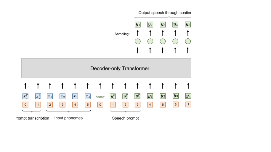
Specifically, in the training process, illustrated in Figure 1(a), the phoneme and speech sequences are concatenated along the time axis and fed into a decoder-only Transformer model. It is assumed that the speaker’s voice remains constant within each training utterance. In the inference phase, as shown in Figure 1(b), a speech prompt ${𝒚}^p$ is required to determine the voice of the generated speech. The phoneme transcription of the speech prompt ${𝒙}^p$ and the speech prompt itself ${𝒚}^p$ are positioned at the beginning of the input and output sequences respectively, followed by the input phonemes to be generated and their corresponding output speech tokens. The process of auto-regressive continuation from the speech prompt is believed to preserve the speaker’s voice in the generated output.

(a) Model architecture.

(b) Monotonic alignment path $\overline{𝒚}$ of length $T+U$.

Figure 2: The model architecture and monotonic alignment path of Transducer.

2.2 Transducer

The Transducer model (Graves, 2012), also known as RNN-T, is designed for monotonic sequence-to-sequence tasks and comprises three components: an encoder, a prediction network, and a joint network. Here, the prediction network is an auto-regressive network, such as RNN and LSTM. Transducer model also introduces a special output token called blank, denoted as $\mathrm{\varnothing }$, which signifies the alignment boundary between output and input sequence. We define $𝒴$ as the vocabulary of output tokens and $\overline{𝒴}=𝒴\cup \{\mathrm{\varnothing }\}$ as the extended vocabulary. Also, we denote the lengths of the input sequence $𝒙$ and output sequence $𝒚$ as $T$ and $U$ and the size of the extended vocabulary $\overline{𝒴}$ as $\overline{V}$.

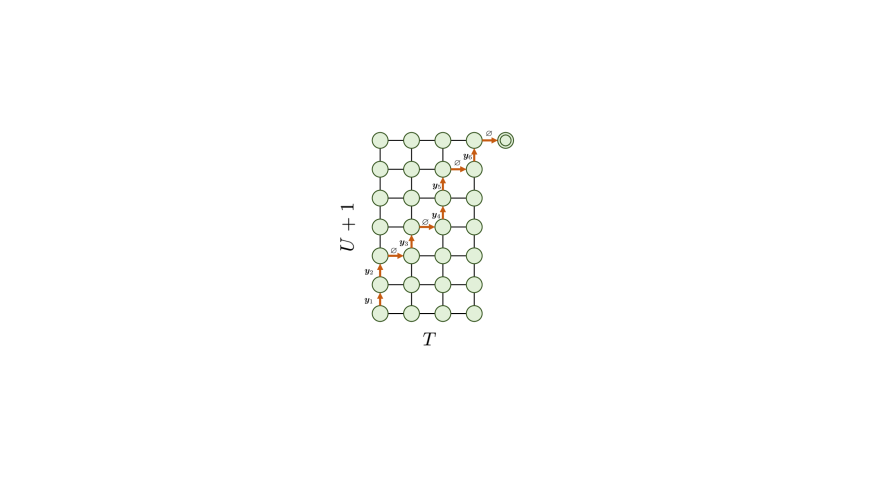
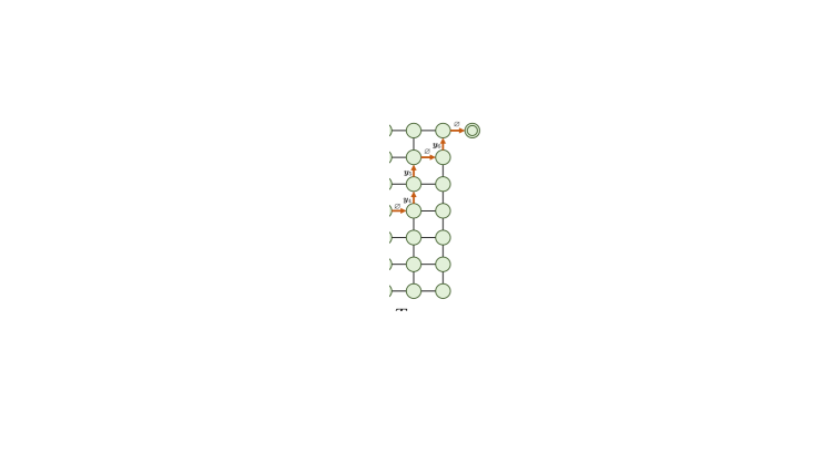
In the training phase, as shown in Figure 2(a), the encoder and prediction network encode the two sequences $𝒙$ and $𝒚$ respectively, yielding encoded hidden sequences $𝒇$ and $𝒈$. Subsequently, we slice the hidden vectors ${𝒇}_t$ and ${𝒈}_u$ at positions $t$ and $u$ respectively, then send them to the joint network to calculate the probability ${𝒑}_{t,u}=\mathrm{𝐏𝐫}({\overline{𝒚}}_{t+u}|{𝒇}_t,{𝒈}_u)$ for the next token prediction, where ${\overline{𝒚}}_{t+u}\in \overline{𝒴}$. We iterate over all possible sliced hidden vectors of the two sequences, from ${𝒇}_0$ to ${𝒇}_{T-1}$ and from ${𝒈}_0$ to ${𝒈}_U$, generating a matrix $𝒑$ of shape $T\times (U+1)$ whose entry at $(t,u)$ is ${𝒑}_{t,u}$. Each path $\overline{𝒚}$ from the bottom left corner to the top right corner represents an alignment between $𝒙$ and $𝒚$, with a length of $T+U$. Figure 2(b) demonstrates an example of the alignment path where $\overline{𝒚}=[{𝒚}_1,{𝒚}_2,\mathrm{\varnothing },{𝒚}_3,\mathrm{\varnothing },{𝒚}_4,{𝒚}_5,\mathrm{\varnothing },{𝒚}_6,\mathrm{\varnothing }]$.

The training criterion of Transducer model is to maximize the probability of $\mathrm{𝐏𝐫}(𝒚|𝒙)$, which is the summation of the probabilities of all possible alignment paths $\overline{𝒚}$, that is

$\mathrm{𝐏𝐫}(𝒚|𝒙)$ $={\displaystyle \sum _{\overline{𝒚}}}\mathrm{𝐏𝐫}(\overline{𝒚}|𝒙)$ (1)

$={\displaystyle \sum _{\overline{𝒚}}}{\displaystyle \prod _{i=0}^{T+U-1}}\mathrm{𝐏𝐫}({\overline{𝒚}}_i|{𝒇}_{t_i},{𝒈}_{u_i})$

where ${𝒇}_{t_i}$ and ${𝒈}_{u_i}$ are sliced hidden vectors at corresponding positions specified by the alignment path $\overline{𝒚}$. In practice, this probability can be effectively calculated with dynamic programming.

In the inference phase, the prediction network auto-regressively predicts the next token, conditioning on the sliced input hidden vectors that slide from ${𝒇}_0$ to ${𝒇}_{T-1}$ whenever the blank token $\mathrm{\varnothing }$ emerges.

The Transducer model has demonstrated remarkable success in ASR. However, its modularized architecture is not suitable enough for generation tasks. Recently, some literatures have explored the application of Transducer to TTS (Chen et al., 2021; Kim et al., 2023), but they still rely on the typical modularized architecture and consequently result in limited performance. Different from the previous works, we propose for the first time to implement Transducer with a decoder-only architecture that achieves better performance.

Figure 3: The training and monotonic auto-regressive inference of VALL-T.

3 VALL-T: Decoder-Only Generative Transducer

Current modularized Transducer model has demonstrated significant success in ASR. Nevertheless, its suitability for generation tasks is limited. Typically, the joint network is a small network, comprising only one or a few linear projection layers, and the prediction network is LSTM or Transformer blocks. This architecture introduces a limitation wherein the input condition $𝒙$ is not incorporated into the generation process until it reaches the joint network. Worse still, the joint network is too small to effectively integrate input conditions into the generation process. Moreover, the modularized Transducer model utilizes slicing to denote specific positions. Consequently, the joint network is unable to explicitly perceive the input context, further making difficulties in achieving satisfactory performance for conditional generation tasks.

To address the above issues, we propose VALL-T that integrates the encoder, the prediction network and the joint network into one single decoder-only Transformer architecture and leverages relative position embedding to denote the corresponding positions. We discuss the training and inference details below.

3.1 Training

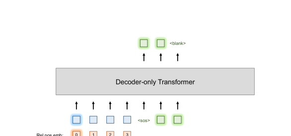
We use a decoder-only architecture for VALL-T. Similar to the approach in the previous work VALL-E, we concatenate the input phoneme and output speech tokens along the time axis and present them to the model as a unified sequence. Unlike traditional RNN and LSTM architectures, the Transformer lacks a specific time order for input tokens, relying instead on position embeddings to indicate their positions. The position indices for the input sequence range from $0$ to $T-1$ and are converted into position embeddings through a sinusoidal function (Vaswani et al., 2017). Similarly, the output sequence adopts position indices from $0$ to $U$, including an additional <sos> token at the beginning. Following VALL-E, we utilize a triangular attention mask for the output sequence, facilitating auto-regressive generation. This mask ensures that each speech token attends to only previously generated tokens, maintaining a proper sequential order in the output.

Beyond the typical absolute position indices starting from 0, we introduce additional relative position indices in VALL-T for input tokens. The relative position index $0$ specifies the current phoneme under synthesis. The phonemes to its left are assigned negative position indices starting from $-1$, while those to its right are assigned positive position indices starting from $1$. These relative position indices are converted to relative position embeddings with a same sinusoidal function as the absolute position indices. The resulting absolute and relative position embeddings are added to the input phoneme embeddings and subsequently presented to the decoder-only Transformer. In adopting this approach, the model gains awareness of the phoneme presently undergoing synthesis, specifically the one assigned a relative position of $0$, and the phonemes serving as its preceding and subsequent contexts.

To eliminate the need for explicit duration modeling, we introduce a special output token called blank, which serves as a marker denoting the end of each phoneme’s generation. Consequently, the output projection following the decoder-only Transformer projects the hidden sequence into a size of $\overline{V}$. The projected hidden sequence, with a length of $U+1$, undergoes a Softmax function to yield a sequence representing the output distribution. Illustrated in Figure 3, we iteratively assign relative position $0$ to each of the $T$ phonemes and subsequently stack every output sequence, each of length $U+1$. This stacking process results in a matrix $𝒑$ of shape $T\times (U+1)$. The optimization of VALL-T utilizes the Transducer loss, calculated using this matrix and the ground-truth speech tokens, to maximize the probability of $p(𝒚|𝒙)$ following Equation (1).

3.2 Monotonic auto-regressive inference

Let us first consider the auto-regressive inference process without a speech prompt. Initially, the relative position $0$ is designated to the first phoneme, starting the speech generation from the <sos> token. The model then auto-regressively produces speech tokens based on the input phoneme tokens and previously generated speech tokens until the blank token $\mathrm{\varnothing }$ emerges. The emergence of $\mathrm{\varnothing }$ denotes the completion of the first phoneme’s generation and triggers a shift in relative positions. We iteratively conduct the above process until the appearance of $\mathrm{\varnothing }$ for the last phoneme, indicating the conclusion of the entire generation process for the input phoneme sequence. Since the model is encouraged to generate speech tokens for the phoneme assigned relative position $0$ by Transducer loss during traning, the step-by-step shifting operation during decoding facilitates the monotonic generation process and consequently enhance the robustness against hallucination.

Next, we consider the integration of the speech prompt for zero-shot speaker adaptation. Following the approach used in VALL-E, the phoneme transcription of the speech prompt is placed at the start of the input sequence, while the speech prompt itself is positioned at the beginning of the output sequence. The two sequences are followed by the input phonemes to be generated and their corresponding output speech tokens respectively. Given that the speech prompt are provided, we assign the relative position 0 to the first phoneme right after the prompt transcription, as shown in Figure 3, and perform speech continuation. Likewise, the relative positions undergo a shift each time $\mathrm{\varnothing }$ emerges, repeating until the generation for the final phoneme is completed.

(a) Forward variable map.

(b) Backward variable map.

(c) Posterior probability map.

(d) Monotonic alignment path.

Figure 4: Alignment analysis with VALL-T given both speech and its transcription.

3.3 Pseudo prompt transcription for untranscribed speech prompt

In previous decoder-only TTS models, the alignment is learned implicitly with self-attentions. These models have to discern which phoneme is currently being synthesized at each time step solely based on the self-attentions between the input tokens and the preceding output tokens. Therefore, they rely on correct transcription of the speech prompt to get correct alignment and start the generation accordingly. However, in practice, it is inconvenient to obtain transcribed speech prompt, so we hope to leverage speech prompt directly and eliminate the need of its transcription.

In VALL-T, it is evident that the alignment is controllable during inference, allowing us to manipulate the generation process by assigning position $0$ to the phoneme we intend to synthesize without relying on a paired speech prompt and its transcription. Accordingly, we can perform zero-shot adaptation with untranscribed speech prompts. Specifically, given an untranscribed speech prompt, we use the phoneme sequence of a random utterance, referred to as pseudo prompt transcription, as its transcription and place it at the beginning of the input sequence. Then the generation can start correctly by leveraging exactly the same algorithm as described in section 3.2. The reason for using a pseudo prompt transcription rather than no prompt transcription lies in the presence of absolute position embeddings in the input sequence. We need to avoid unseen alignment pattern in the view of absolute position embeddings.

Moreover, since there is no necessity for transcribing the speech prompt, the utilization of untranscribed speech prompts can be expanded to include prompts in unknown languages. This enables cross-lingual zero-shot adaptive speech synthesis.

3.4 Aligned context window for lengthy speech synthesis

Decoder-only Transformer models have very limited ability to generalize to unseen position embeddings. That means if we are synthesizing lengthy speech that exceeds the maximum length encountered during training, the performance would be degraded.

Fortunately, in VALL-T, the alignment is available during inference, allowing us to employ aligned context window that constrains both the input and output sequence length simultaneously. Specifically, at each decoding step, we retain only $n$ phonemes that precede the current phoneme and $m$ phonemes that follow it, creating a constrained sliding context window on input phonemes. Also, we preserve only the speech tokens corresponding to the $n$ preceding phonemes given the alignment and discard more distant history, forming a context window on the output sequence as well. Hence, by leveraging aligned context window, VALL-T consistently maintains a limited context on both input and output sequence, allowing it to generate speech of any lengths.

4 Experiments and Results

4.1 Setup

In our experiments, we leverage our Encodec (Défossez et al., 2022) speech tokenizer whose frame shift is 20ms and the sampling rate of output waveforms is 16k. It comprises 8 residual vector quantization (RVQ) indices for each frame. To ensure a fair comparison between VALL-E and our proposed model VALL-T, we follow the approach introduced in VALL-E that predicts the sequence of the first RVQ index with the auto-regressive models and then predicts the remaining 7 RVQ indices conditioned on the first RVQ index with a separate non-auto-regressive (NAR) model. Both the input and output sequences are encoded with BPE (Sennrich et al., 2016) algorithm to shorten sequence lengths and diminish GPU memory consumption. VALL-T adopts an identical architecture to VALL-E, containing 12 layers of Transformer blocks. Each block comprises 12 attention heads and has a hidden dimension of 1024.

We use LibriTTS (Zen et al., 2019) dataset in our experiments, which is a multi-speaker transcribed English speech dataset. Its training set consists of approximately 580 hours of speech data from 2,306 speakers. We train our model for 40 epochs using a ScaledAdam (Yao et al., 2023) optimizer. The learning rate scheduler is Eden (Yao et al., 2023) with a base learning rate of $0.05$, an epoch scheduling factor of 4 and a step scheduling factor of 5000.

4.2 Alignment analysis

We first do alignment analysis to check if relative position embedding in VALL-T indicates the alignment as expected. Given the speech $𝒚$ and its transcription $𝒙$, we iterate over all relative positions and calculate the matrix $𝒑$ of output distributions in the shape of $T\times (U+1)$. Then we calculate the forward variables, backward variables and posterior probabilities accordingly. The concepts of forward variable, backward variables, and posterior probabilities were initially introduced in Hidden Markov Models (Young et al., 2002) and were also introduced in Transducer (Graves, 2012). The definitions and calculation for these values are elaborated in Appendix A.

Table 1: The performance of zero-shot TTS.

Method	WER(%) $\downarrow$	MCD $\downarrow$	Naturalness MOS $\uparrow$	Similarity MOS $\uparrow$	SECS $\uparrow$
Ground-truth	1.92	0	4.63 $\pm$ 0.07	4.23 $\pm$ 0.10	0.837
Encodec resynthesis	2.08	2.50	4.55 $\pm$ 0.07	4.19 $\pm$ 0.11	0.835
NAR resynthesis	3.75	2.95	4.44 $\pm$ 0.07	4.24 $\pm$ 0.10	0.846
Transduce and Speak	6.14	4.38	4.07 $\pm$ 0.10	4.02 $\pm$ 0.11	0.838
VALL-E	5.80	4.00	4.25 $\pm$ 0.08	4.12 $\pm$ 0.10	0.857
VALL-T (ours)	4.16	3.98	4.26 $\pm$ 0.08	4.21 $\pm$ 0.09	0.849

Table 2: Zero-shot TTS with untranscribed speech prompt. The three baselines fail to generate the speech correctly, resulting in much higher WERs. We do not conduct MOS tests on the three baselines since it makes no sense to assess the naturalness and similarity for entirely incorrect generated audio samples.

Method	Pseudo Prompt	WER(%) $\downarrow$	MCD $\downarrow$	Naturalness MOS $\uparrow$	Similarity MOS $\uparrow$	SECS $\uparrow$
	Transcription
VALL-E	$\times$	68.22	4.97	-	-	0.795
	$\surd$	21.01	4.28	-	-	0.836
VALL-T	$\times$	30.86	4.43	-	-	0.836
	$\surd$	3.48	3.97	4.29 $\pm$ 0.09	4.14 $\pm$ 0.10	0.848

In Figure 4, we illustrate an example of the forward variable, backward variable, and posterior probability for VALL-T, with darker colors indicating lower values. The values are plotted on a logarithmic scale. In Figure 4(a) and 4(b), we can see a faint bright line on the diagonal of the two graphs.

Table 3: Zero-shot TTS with untranscribed speech prompt in unknown languages.

Method	WER(%) $\downarrow$	Naturalness MOS $\uparrow$	Similarity MOS $\uparrow$	SECS $\uparrow$
VALL-E	39.83	-	-	0.779
VALL-T	4.22	4.25 $\pm$ 0.08	4.36 $\pm$ 0.06	0.782

Table 4: Evaluation on generating lengthy speech that exceeds the maximum length encountered during training.

Method	Aligned Context	WER(%) $\downarrow$	MCD $\downarrow$	Naturalness MOS $\uparrow$	Similarity MOS $\uparrow$	SECS $\uparrow$
	Window
Ground-truth	-	1.68	2.50	4.81 $\pm$ 0.05	4.48 $\pm$ 0.09	0.877
VALL-E	$\times$	50.82	4.37	-	-	0.875
VALL-T	$\times$	14.63	4.31	4.21 $\pm$ 0.08	4.31 $\pm$ 0.07	0.828
VALL-T	$\surd$	5.50	4.26	4.39 $\pm$ 0.06	4.37 $\pm$ 0.07	0.847

Pixel-wise summing the values from Figure 4(a) and Figure 4(b) produces Figure 4(c), which represents the posterior probability. The diagonal line becomes much clearer in this composite figure, indicating that VALL-T correctly models the alignment between the input and output sequences with relative position embeddings. Accordingly, VALL-T is capable of forced alignment, where the most probable path from the bottom-left corner to the top-right corner in the posterior probability map serves as the alignment path. The alignment path for this example is depicted in Figure 4(d). Since ground-truth labels for alignment are unavailable, our alignment analysis here only focuses on qualitative aspects.

4.3 Evaluation on zero-shot TTS

In this section, we conduct an evaluation of our models on zero-shot TTS task. The task refers to synthesizing speech in the voices of unseen speakers given speech prompts and their corresponding transcriptions. Our test set uses a same test set as in (Du et al., 2024), containing 500 utterances and involving 37 speakers from the LibriTTS test set. Each speaker is assigned a specific speech prompt. Before assessing the performance of our models, we conduct speech resynthesis using our Encodec to evaluate the speech tokenizer. We also do an experiment named “NAR resynthesis”. In this experiment, we send the ground-truth first RVQ index to the NAR model for predicting the remaining 7 RVQ indices. Then, we convert all the 8 RVQ indices to waveform using the Encodec decoder. The purpose of the NAR resynthesis experiment is to demonstrate the performance degradation introduced by the NAR model, so we can better analyze the results of the entire pipelines, where the AR models are the primary focus of our paper.

The baselines of this experiment include two models. One is the popular decoder-only TTS model VALL-E and another is the recently proposed TTS model with a modularized Transducer achitecture called “Transduce and Speak” (Kim et al., 2023). The main evaluation metric in this paper is the word error rate (WER). In our evaluation process, we first synthesize speech for the test set, and then perform speech recognition using a well-known ASR model, Whisper (Radford et al., 2023). The transcriptions obtained from the ASR model are then compared to the ground-truth input text to calculate the word error rate. Table 1 shows that VALL-T attains significant lower WER than baselines, which is a 28.3% relative reduction when compared to VALL-E and is only 0.41 higher than NAR resynthesis, suggesting the robustness of VALL-T.

Additionally, we present the mel-cepstral distortion (MCD) in the table, serving as a metric for quantifying the distance between the generated speech and the corresponding ground-truth recordings. VALL-T also achieves the lowest MCD across all models. Further evaluations extend to Mean Opinion Score (MOS) listening tests for naturalness and speaker similarity. 15 listeners were tasked with rating each utterance on a scale from 1 to 5, with higher scores indicating better naturalness and similarity. Note that the speaker similarity is evaluated between the generated speech and the provided speech prompt, not the corresponding ground-truth speech. This distinction arises from the variability in a speaker’s timbre across different utterances, and the goal is to emulate solely the timbre of the given prompt. In the listening tests, VALL-T achieves a naturalness score comparable to VALL-E, with a slightly better speaker similarity. Finally, the evaluation extends to the calculation of Speaker Embedding Cosine Similarity (SECS), measured using a pretrained speaker verification model. This metric measures the speaker similarity by assessing the cosine similarity between the speaker embeddings of the generated speech and the provided speech prompt. While VALL-T exhibits a marginally lower SECS value than VALL-E, it still surpasses other models and does not detrimentally affect human perception according to the results of subjective listening tests on similarity.

4.4 Leveraging untranscribed speech prompt

The alignment controllability of VALL-T allow us to leverage untranscribed speech prompts for zero-shot TTS. In this experiment, we still use a same test set as in the previous section, excluding the transcription of the speech prompts to simulate a scenario where prompt transcriptions are unavailable. One utterance is randomly chosen from the LibriTTS test set, and its phoneme transcription serves as the pseudo prompt transcription for generating all utterances in the test set. We compare the proposed approach with three baselines. The first baseline is generating with VALL-T but do not use any prompt transcription. The remaining two baselines use VALL-E, one utilizing pseudo prompt transcriptions and the other using no prompt transcription.

The results are presented in Table 2. We find VALL-E consistently fails to perform continuation in the absence of the correct prompt transcription, regardless of whether pseudo prompt transcriptions are provided or not. Although VALL-T exhibits improved robustness, it still fails in continuation tasks when no prompt transcription is used. This failure is caused by the unseen alignment pattern in the view of absolute position embeddings. When provided with pseudo prompt transcriptions, VALL-T successfully accomplishes the continuation from the speech prompt. The WER is significantly lower than the three baselines and even lower than both the results obtained using real prompt transcription and using NAR resynthesis in Table 1. This improvement may be attributed to the reduced noise in the fixed pseudo prompt transcription compared to the diverse real prompt transcriptions. This result further demonstrate the robustness of VALL-T.

Similarly, we observe a lower MCD compared with other baselines with the proposed approach. We do not conduct listening tests on the three baselines since it makes no sense to assess the naturalness and similarity for entirely incorrect generated audio samples. The naturalness of the proposed approach is almost the same as that observed when using real prompt transcriptions while its speaker similarity is slightly lower. We can also observe that in SECS evaluation.

Next, we extend the utilization of untranscribed speech prompts to those spoken in unknown languages. Specifically, we continue to use the same test set as in the previous experiments, but leverage speech prompts from 10 German and 10 Spanish speakers randomly selected from the Multilingual Librispeech dataset (Pratap et al., 2020), simulating the speech prompt in unknown languages. Employing the same English pseudo prompt transcription as in the previous experiment for both VALL-T and the baseline VALL-E, we generate continuations from the speech prompts in German and Spanish. The results are posted in Table 3. VALL-E continues to fail in the generation due to the unknown prompt transcription. On the contrary, VALL-T still successfully performs the zero-shot TTS from the speech prompts in German and Spanish, achieving a WER of 4.22. Note that the similarity MOS and SECS in this experiment cannot be directly compared with the corresponding results in Table 1 and 2 since the speakers of the speech prompts differ. We do not have corresponding ground-truth speech that speaks the utterances in the test set in the voice of German and Spanish speakers, so we also do not calculate the MCD in this experiment.

4.5 Evaluate on lengthy speech generation

We also evaluate our model on lengthy speech synthesis that exceeds the maximum length encountered during training. Due to the limitation of GPU memory, the maximum duration of training utterances is approximately 15 seconds. The test set for this experiment consists of 85 utterances, each formed by concatenating five utterances from the previous test set to simulate lengthy utterance. The generated speech in this test set exceeds 20 seconds. We use $n=50$ and $m=15$ as the context window size.

Examining the results in Table 4, we observe that VALL-T exhibits superior generalization to long speech compared to VALL-E, attributed to its utilization of relative position embedding, even in the absence of an aligned context window. In contrast, VALL-E often starts mumbling after generating approximately 20 seconds of speech and frequently terminates prematurely without completing the generation. Upon applying the aligned context window, the WER of VALL-T further decreases and approaches the result of generating normal utterances. Additionally, the gap in MOS scores for naturalness and speaker similarity between generated speech and ground-truth is also comparable to the result of synthesizing normal utterances.

5 Conclusion

In this research, we present VALL-T, a decoder-only generative Transducer model designed to improve the robustness and controllability of TTS models. VALL-T incorporates monotonic alignment constraints into the decoder-only TTS framework, enabling implicit modeling of phoneme durations. Threfore, this model eliminates the need for acquiring phoneme durations before training. VALL-T supports forced alignment given input phonemes and the corresponding output speech by searching the best path on the posterior probability map. This alignment is controllable during inference, facilitating zero-shot synthesis with untranscribed speech prompts even in unknown languages. Additionally, VALL-T exhibits the capability of streaming generation, coupled with an aligned context window for synthesizing lengthy speech. These features make VALL-T a powerful model for TTS applications.

Appendix A Forward variable, backward variable and posterior probability in Transducer.

In Section 4.2, we analyze the alignment by calculating the forward variable, backward variable and the posterior probability. In this section, we provide additional details into the definition and calculation of these variables.

The forward variable at position $(t,u)$ is denoted as $\alpha (t,u)$, representing the probability of observing the output ${𝒚}_{1:u}=[{𝒚}_1,\mathrm{\dots },{𝒚}_u]$ given the input ${𝒙}_{1:t+1}$, where $0\le u\le U$ and $0\le t\le T-1$. In other words, it is the summation of probabilities of all paths starting from $(0,0)$ and ending at $(t,u)$.

Due to the computational complexity of calculating probabilities for all possible paths, dynamic programming is employed for efficiency. The calculation of the forward variable begins by initializing $\alpha (0,0)=1$. Subsequently, the forward variable at each position is computed inductively based on its left and below entries:

$\alpha (t,u)=$ $\alpha (t-1,u)\times {𝒑}_{t-1,u}[\mathrm{\varnothing }]$ (2)

$+\alpha (t,u-1)\times {𝒑}_{t,u-1}[{𝒚}_u].$

By calculating the forward variables, we can also know the probability of $\mathrm{𝐏𝐫}(𝒚|𝒙)$ defined in Equation 1 by

$\mathrm{𝐏𝐫}(𝒚|𝒙)=\alpha (T-1,U).$ (3)

Similarly, we denote backward variable at position $(t,u)$ as $\beta (t,u)$, representing the probability of observing the output ${𝒚}_{u+1:U}=[{𝒚}_{u+1},\mathrm{\dots },{𝒚}_U]$ given ${𝒙}_{t+1:T}$. In other words, it is the summation of probabilities of all paths from $(t,u)$ to $(T-1,U)$.

Backward probability can also be calculated with dynamic programming effectively but in the reverse direction. We start from $\beta (T-1,U)={𝒑}_{T-1,U}[\mathrm{\varnothing }]$ and compute the backward variable at each position inductively based on its above and right entries:

$\beta (t,u)=$ $\beta (t+1,j)\times {𝒑}_{t,u}[\mathrm{\varnothing }]$ (4)

$+\beta (t,u+1)\times {𝒑}_{t,u}[{𝒚}_{u+1}].$

Finally, we define posterior probability $\gamma (t,u)$ to be the probability of producing ${𝒚}_{1:u}$ until time step $t$ given the entire input and output sequence $𝒙$ and $𝒚$. In other words, it is the summation of probabilities of all paths starting from $(0,0)$, passing through the point $(t,u)$ and ending at $(T-1,U)$. Posterior probability $\gamma$ can be readily computed by multiplying the forward and backward variables, that is

$$\gamma (t,u)=\alpha (t,u)\times \beta (t,u).$$ (5)

The posterior probability suggests the potential alignment relationship between the two sequences $𝒙$ and $𝒚$. We plot an example map of these values in Figure 4.

(a) Bad case with word repeating in VALL-E.

(b) Corresponding sample from VALL-T without word repeating.

Figure 5: Illustration of an example of bad case with word repeating in VALL-E. The input transcription is “I should torture myself-I couldn’t help it." After that it was easy to forget, actually to forget.”

(a) Bad case with word skipping in VALL-E.

(b) Corresponding sample from VALL-T without word skipping.

Figure 6: Illustration of an example of bad case with word skipping in VALL-E. The input transcription is “He was particularly attentive to the behavior of their preachers, on whom all depended.”

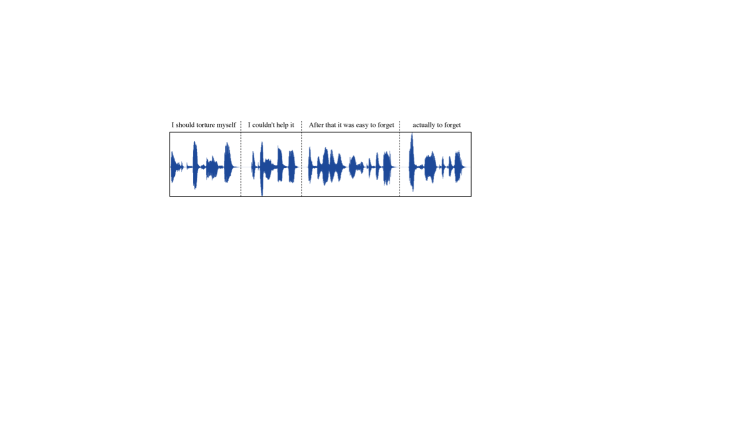
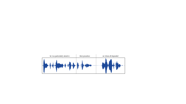
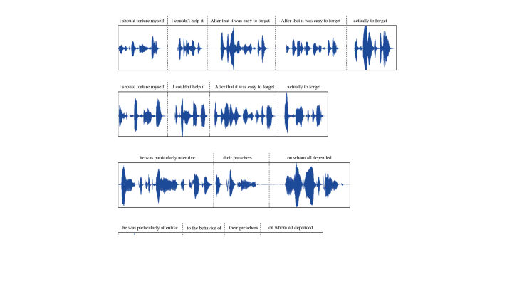
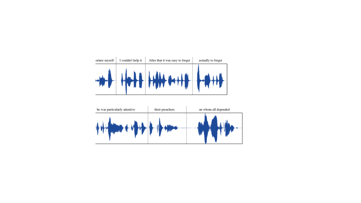
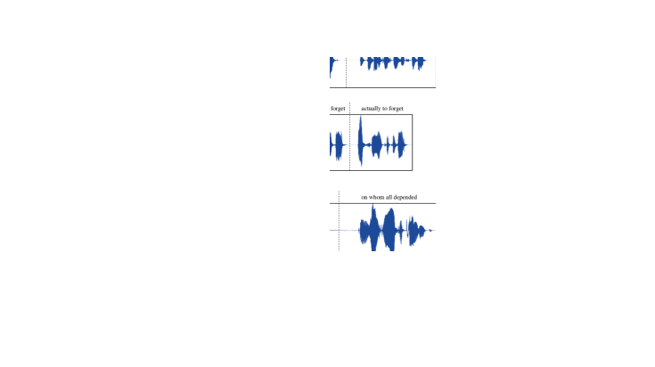
Appendix B Illustration of hallucination issues in VALL-E.

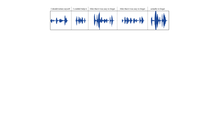
In Section 4.3, it is observed that VALL-E sometimes suffer from hallucination issues. This section illustrates some examples of these occurrences by plotting the waveforms of the audio samples alongside their corresponding transcriptions.

Figure 5(a) depicts an audio sample with word repeating from VALL-E. In this example, a phoneme segment is spoken twice, separated by a short silence. In contrast, when this utterance is presented to VALL-T, the generation is correct without any repeating, as demonstrated in Figure 5(b).

We also illustrate an audio sample of word skipping from VALL-E in Figure 6(a). In this example, an input segment is skipped over. Similarly, when this utterance is presented to VALL-T, no skipping occurs as depicted in Figure 6(b).

Appendix C History context window size in lengthy speech generation.

In Section 4.5, we evaluate the models on lengthy speech synthesis, where the future context size $m$ is restricted to a specified value of $15$ to facilitate streaming generation. Consequently, this section investigates only the influence of the history context size $n$ on the generated outputs.

Figure 7: The curve of word error rate with different history context size $n$.

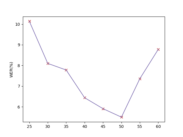
We plot the curve of word error rate with different history context size in Figure 7. We can see from the plot that the WER initially decreases as the history context size grows. This observation aligns with our intuition, as a more history context provides the model with additional information, enabling more informed decisions during the decoding process. However, beyond a certain threshold, we observe a subsequent increase in the WER. This phenomenon can be attributed to the challenges arising from the complexity of too long speech sequences. Therefore, in streaming generation with aligned context window, we need to determine the optimal historical context size for achieving the best performance.

Appendix D Pseudo code for VALL-T.

In Section 3.1 and 3.2, we introduce the training and zero-shot inference algorithms of VALL-T. Here we present their corresponding pseudo codes in Algorithm 1 and 2.

Algorithm 1 Training of VALL-T within one iteration.

Input: A batch of training data $\{({𝒙}^{(1)},{𝒚}^{(1)}),({𝒙}^{(2)},{𝒚}^{(2)}),\mathrm{\dots },({𝒙}^{(B)},{𝒚}^{(B)})\}$.
Parameter: Optimizer $optim$, model parameters $\theta$.

1: $loss=0$

2: for $i=1,2,\mathrm{\dots },B$ do

3: $T=\text{len}({𝒙}^{(i)})$

4: $U=\text{len}({𝒚}^{(i)})$

5: $abs\mathrm{\_}pos\mathrm{\_}emb\mathrm{\_}x=[0,1,2,\mathrm{\dots },T-1]$

6: $abs\mathrm{\_}pos\mathrm{\_}emb\mathrm{\_}y=[0,1,2,\mathrm{\dots },U]$

7: for $t=0,1,2,\mathrm{\dots },T-1$ do

8: $rel\mathrm{\_}pos\mathrm{\_}emb\mathrm{\_}x=[0-t,1-t,2-t,\mathrm{\dots },T-1-t]$

9:

10: ${𝒑}_{t,0:U}=out[-(U+1):]$

11: end for

12: $loss=loss+\text{TransducerLoss}({𝒑}_{0:T-1,0:U},{𝒚}^{(i)})$

13: end for

14: $loss.\text{backward}()$

15: $optim.\text{step}()$

Algorithm 2 Zero-shot inference of VALL-T.

Input: Phoneme sequence $𝒙$, speech prompt ${𝒚}^p$ and speech prompt transcription ${𝒙}^p$.
Parameter: Model parameters $\theta$.
Output: Speech token sequence $𝒚$ corresponding to $𝒙$.

1: $T=\text{len}(𝒙)$

2: $T^p=\text{len}({𝒙}^p)$

3: $U^p=\text{len}({𝒚}^p)$

4: $𝒚=[]$

5: $abs\mathrm{\_}pos\mathrm{\_}emb\mathrm{\_}x=[0,1,2,\mathrm{\dots },T+T^p-1]$

6: for $t=0,1,2,\mathrm{\dots },T-1$ do

7: $rel\mathrm{\_}pos\mathrm{\_}emb\mathrm{\_}x=[0-T^p-t,1-T^p-t,2-T^p-t,\mathrm{\dots },T-1-t]$

8: while True do

9: $u=\text{len}(𝒚)$

10: $abs\mathrm{\_}pos\mathrm{\_}emb\mathrm{\_}y=[0,1,2,\mathrm{\dots },U^p+u]$

11:

12: ${\overline{𝒚}}_{t+u}=\text{Sampling}(out[-1])$

13: if ${\overline{𝒚}}_{t+u}$ == $\mathrm{\varnothing }$ then

14: break

15: else

16: ${𝒚}_{u+1}={\overline{𝒚}}_{t+u}$

17: $𝒚=\text{Concat}(𝒚,[{𝒚}_{u+1}])$

18: end if

19: end while

20: end for

21: return $𝒚$

References

- Betker (2023) Betker, J. Better speech synthesis through scaling. arXiv preprint arXiv:2305.07243, 2023.
- Brown et al. (2020) Brown, T. B., Mann, B., Ryder, N., et al. Language models are few-shot learners. In NeurIPS, 2020.
- Chen et al. (2021) Chen, J., Tan, X., Leng, Y., Xu, J., Wen, G., Qin, T., and Liu, T. Speech-T: Transducer for text to speech and beyond. In NeurIPS, pp. 6621–6633, 2021.
- Défossez et al. (2022) Défossez, A., Copet, J., Synnaeve, G., and Adi, Y. High fidelity neural audio compression. arXiv preprint arXiv:2210.13438, 2022.
- Du et al. (2022) Du, C., Guo, Y., Chen, X., and Yu, K. VQTTS: high-fidelity text-to-speech synthesis with self-supervised VQ acoustic feature. In ISCA Interspeech, pp. 1596–1600, 2022.
- Du et al. (2024) Du, C., Guo, Y., Shen, F., Liu, Z., Liang, Z., Chen, X., Wang, S., Zhang, H., and Yu, K. UniCATS: A unified context-aware text-to-speech framework with contextual vq-diffusion and vocoding. AAAI, 2024.
- Graves (2012) Graves, A. Sequence transduction with recurrent neural networks. arXiv preprint arXiv:1211.3711, 2012.
- Guo et al. (2024) Guo, Y., Du, C., Ma, Z., Chen, X., and Yu, K. VoiceFlow: Efficient text-to-speech with rectified flow matching. IEEE ICASSP, 2024.
- He et al. (2019) He, Y., Sainath, T. N., Prabhavalkar, R., et al. Streaming end-to-end speech recognition for mobile devices. In IEEE ICASSP, pp. 6381–6385, 2019.
- Kharitonov et al. (2023) Kharitonov, E., Vincent, D., Borsos, Z., et al. Speak, read and prompt: High-fidelity text-to-speech with minimal supervision. arXiv preprint arXiv:2302.03540, 2023.
- Kim et al. (2023) Kim, M., Jeong, M., Choi, B. J., Lee, D., and Kim, N. S. Transduce and speak: Neural transducer for text-to-speech with semantic token prediction. IEEE ASRU, 2023.
- Lakhotia et al. (2021) Lakhotia, K., Kharitonov, E., Hsu, W.-N., Adi, Y., Polyak, A., Bolte, B., Nguyen, T.-A., Copet, J., Baevski, A., Mohamed, A., et al. On generative spoken language modeling from raw audio. Transactions of the Association for Computational Linguistics, 9:1336–1354, 2021.
- Popov et al. (2021) Popov, V., Vovk, I., Gogoryan, V., Sadekova, T., and Kudinov, M. A. Grad-TTS: A diffusion probabilistic model for text-to-speech. In ICML, volume 139, pp. 8599–8608, 2021.
- Pratap et al. (2020) Pratap, V., Xu, Q., Sriram, A., Synnaeve, G., and Collobert, R. MLS: A large-scale multilingual dataset for speech research. In ISCA Interspeech, pp. 2757–2761, 2020.
- Radford et al. (2023) Radford, A., Kim, J. W., Xu, T., Brockman, G., McLeavey, C., and Sutskever, I. Robust speech recognition via large-scale weak supervision. In ICML, volume 202, pp. 28492–28518, 2023.
- Ren et al. (2020) Ren, Y., Hu, C., Tan, X., Qin, T., Zhao, S., Zhao, Z., and Liu, T.-Y. Fastspeech 2: Fast and high-quality end-to-end text to speech. arXiv preprint arXiv:2006.04558, 2020.
- Sennrich et al. (2016) Sennrich, R., Haddow, B., and Birch, A. Neural machine translation of rare words with subword units. In ACL, 2016.
- Touvron et al. (2023) Touvron, H., Martin, L., Stone, K., et al. Llama 2: Open foundation and fine-tuned chat models. arXiv preprint arXiv:2005.14165, 2023.
- Vaswani et al. (2017) Vaswani, A., Shazeer, N., Parmar, N., et al. Attention is all you need. In NIPS, pp. 5998–6008, 2017.
- Wang et al. (2023a) Wang, C., Chen, S., Wu, Y., et al. Neural codec language models are zero-shot text to speech synthesizers. arXiv preprint arXiv:2301.02111, 2023a.
- Wang et al. (2023b) Wang, J., Du, Z., Chen, Q., et al. Lauragpt: Listen, attend, understand, and regenerate audio with GPT. arXiv preprint arXiv:2310.04673, 2023b.
- Yao et al. (2023) Yao, Z., Guo, L., Yang, X., Kang, W., Kuang, F., Yang, Y., Jin, Z., Lin, L., and Povey, D. Zipformer: A faster and better encoder for automatic speech recognition. ICLR, 2310.11230, 2023.
- Young et al. (2002) Young, S., Evermann, G., Gales, M., Hain, T., Kershaw, D., Liu, X., Moore, G., Odell, J., Ollason, D., Povey, D., et al. The HTK book. Cambridge university engineering department, 3(175):12, 2002.
- Zen et al. (2019) Zen, H., Dang, V., Clark, R., Zhang, Y., Weiss, R. J., Jia, Y., Chen, Z., and Wu, Y. LibriTTS: A corpus derived from librispeech for text-to-speech. In ISCA Interspeech, pp. 1526–1530, 2019.