Smaug: Fixing Failure Modes of Preference Optimisation with DPO-Positive

Abstract

Direct Preference Optimisation (DPO) is effective at significantly improving the performance of large language models (LLMs) on downstream tasks such as reasoning, summarisation, and alignment. Using pairs of preferred and dispreferred data, DPO models the relative probability of picking one response over another. In this work, first we show theoretically that the standard DPO loss can lead to a reduction of the model’s likelihood of the preferred examples, as long as the relative probability between the preferred and dispreferred classes increases. We then show empirically that this phenomenon occurs when fine-tuning LLMs on common datasets, especially datasets in which the edit distance between pairs of completions is low. Using these insights, we design DPO-Positive (DPOP), a new loss function and training procedure which avoids this failure mode. Surprisingly, we also find that DPOP significantly outperforms DPO across a wide variety of datasets and downstream tasks, including datasets with high edit distances between completions. By fine-tuning with DPOP, we create and release Smaug-34B and Smaug-72B, which achieve state-of-the-art open-source performance. Notably, Smaug-72B is nearly 2% better than any other open-source model on the HuggingFace Open LLM Leaderboard and becomes the first open-source LLM to surpass an average accuracy of 80%.

1 Introduction

Aligning large language models (LLMs) with human preferences is important for their fluency and applicability to many tasks, with the natural language processing literature using many techniques to incorporate human feedback [Christiano et al., 2017, Stiennon et al., 2020, Ouyang et al., 2022]. Typically in LLM alignment, we first collect large amounts of preference data, consisting of a context and two potential completions; one of these is labelled as the preferred completion, and the other as the dispreferred. We use this data to learn a general policy for generating completions in a given context. Direct Preference Optimisation (DPO) [Rafailov et al., 2023] is a popular method for learning from human preferences, and it has shown to be effective at improving the performance of pretrained LLMs on downstream tasks such as reasoning, summarisation, and alignment [Wang et al., 2023, Tunstall et al., 2023]. The theoretical motivation for DPO is based on a preference-ranking model with an implicit reward function that models the relative probability of picking the preferred completion over the dispreferred.

Figure 1: DPOP avoids a failure mode of DPO. When preference pairs differ on only a few tokens, DPO receives no loss incentive at all for the early tokens, and a loss incentive that in some cases can lead to degradation of the log-probs of later tokens (Section 3). We introduce DPOP, which adds a new term to the loss which leads every token to be incentivised toward the preferred completion (Section 4).

In this work, first we show theoretically that the standard DPO loss can lead to a reduction of the model’s likelihood of the preferred completions (as long as the relative probability between the preferred and dispreferred classes increases), and we empirically show that this phenomenon occurs when fine-tuning current LLMs on common datasets. Our theoretical explanation for the phenomenon suggests that the problem occurs most frequently in preference datasets with small edit distances between each pair of completions, such as in math-based preference datasets.

Using these insights, we design a new loss function: DPO-Positive (DPOP), which adds a new term to the loss function that penalises reducing the probability of the positive completions. We also create new preference datasets based on ARC [Clark et al., 2018], HellaSwag [Zellers et al., 2019], and MetaMath [Yu et al., 2023] and use them along with DPOP to create new models.

We introduce the Smaug class of models which use DPOP and achieve state-of-the-art open-source performance. We fine-tune 72B, 34B, and 7B models on our new datasets and show that DPOP far outperforms DPO. We evaluate our resulting models on multiple benchmarks including the HuggingFace Open LLM Leaderboard [Beeching et al., 2023, Gao et al., 2021], which aggregates six popular benchmarks such as MMLU [Hendrycks et al., 2021] and GSM8K [Cobbe et al., 2021], and MT-Bench [Zheng et al., 2023], a challenging benchmark that uses a strong LLM to score candidate model responses across eight different categories of performance. On the HuggingFace Open LLM Leaderboard, Smaug-72B achieves an average accuracy of 80.48%, becoming the first open-source LLM to surpass an average accuracy of 80% and improving by nearly 2% over the second-best open-source model, and our Smaug-34B model is the best in its class of models of similar parameter count. We release our code and pretrained models at https://github.com/abacusai/smaug.

Our contributions.

• We theoretically and empirically show a surprising failure mode of DPO: running DPO on preference datasets with small edit distances between completions can result in a catastrophic decrease in accuracy.

• We introduce DPO-Positive (DPOP) which we theoretically and empirically show ameliorates the performance degradation. In particular, DPOP often outperforms DPO, even on preference datasets with high edit distances between completions.

• We create new preference-based versions of ARC, HellaSwag, and MetaMath.

• Using DPOP and our new datasets, we create and release the Smaug class of models, with Smaug-72B becoming the first open-source model to achieve an average accuracy of 80% on the HuggingFace Open LLM Leaderboard. We open-source our trained models, datasets, and code.

2 Background and Related Work

Large language models (LLMs) have shown impressive zero-shot and few-shot performance [Radford et al., 2019, Brown et al., 2020, Bubeck et al., 2023]. Recently, researchers have fine-tuned pretrained LLMs on downstream tasks by using human-written completions [Chung et al., 2022, Mishra et al., 2021] or by using datasets labelled with human-preferred completions relative to other completions [Ouyang et al., 2022, Bai et al., 2022, Ziegler et al., 2020]. These techniques have been used to improve performance on a variety of downstream tasks such as translation [Kreutzer et al., 2018] and summarisation [Stiennon et al., 2020], as well as to create general-purpose models such as Zephyr [Tunstall et al., 2023]. Two of the most popular techniques for learning from human preference data are reinforcement learning from human feedback (RLHF) [Ouyang et al., 2022, Bai et al., 2022, Ziegler et al., 2020] and direct preference optimisation (DPO) [Rafailov et al., 2023]. We summarise these approaches below.

RLHF

Consider a dataset of pairwise-preference ranked data $𝒟={\{x^{(i)},y_w^{(i)},y_l^{(i)}\}}_{i=1}^N$ where $x^{(i)}$ are prompts and $y_w^{(i)}$ and $y_l^{(i)}$ are respectively the preferred and dispreferred completions conditioned on that prompt. We have an initial LLM ${\pi }_{\text{ref}}$ that parameterises a distribution ${\pi }_{\text{ref}}(y|x)$. Often, we initialise ${\pi }_{\text{ref}}$ as an LLM that has undergone supervised fine-tuning (SFT) to improve performance on downstream task(s).

RLHF begins by modelling the probability of preferring $y_w$ to $y_l$ using the Bradley-Terry model [Bradley and Terry, 1952] which posits the following probabilistic form:

$$p(y_w\succ y_l|x)=\sigma (r(x,y_w)-r(x,y_l))$$

where $\sigma$ is the logistic function and $r(x,y)$ corresponds to some latent reward function that is assumed to exist for the completion $y$ given the prompt $x$. Given $𝒟$, we can learn a parameterised estimate of $r$ by minimising the negative log-likelihood of the dataset:

$${ℒ}_R(r_{\varphi },𝒟)=-{𝔼}_{(x,y_w,y_l)\sim 𝒟}[\log (\sigma (r_{\varphi }(x,y_w)-r_{\varphi }(x,y_l))].$$

For RLHF, we use reinforcement learning to optimise based on this learned reward function $r_{\varphi }$ (with a regularising KL-constraint to prevent model collapse), and obtain a new LLM distribution ${\pi }_{\theta }$.

DPO

Rafailov et al. [2023] showed that it is possible to optimise the same KL-constrained reward function as in RLHF without having to learn an explicit reward function. Instead, the problem is cast as a maximum likelihood optimisation of the distribution ${\pi }_{\theta }$ directly, with the objective:

$${ℒ}_{\text{DPO}}({\pi }_{\theta };{\pi }_{\text{ref}})=-{𝔼}_{(x,y_w,y_l)\sim D}\left[\log \sigma \left(\beta \log \frac{{\pi }_{\theta }(y_w|x)}{{\pi }_{\text{ref}}(y_w|x)}-\beta \log \frac{{\pi }_{\theta }(y_l|x)}{{\pi }_{\text{ref}}(y_l|x)}\right)\right]$$ (1)

where $\beta$ is a regularisation term corresponding to the strength of KL-regularisation in RLHF. In this case, the implicit reward parameterisation is $r(x,y)=\beta \log \frac{{\pi }_{\theta }(y|x)}{{\pi }_{\text{ref}}(y|x)}$, and Rafailov et al. [2023] further showed that all reward classes under the Plackett-Luce model [Plackett, 1975, Luce, 2005] (such as Bradley-Terry) are representable under this parameterisation. For an abbreviation, we define ${\pi }_{\text{ratio}}(y|x)=\frac{{\pi }_{\theta }(y|x)}{{\pi }_{\text{ref}}(y|x)}.$

Since the release of DPO, various alternatives have been proposed. We discuss the most relevant to our work below and in Appendix A.

IPO

Azar et al. [2023] aim to understand the theoretical underpinnings of RLHF and DPO. They identify that DPO may be prone to overfitting in situations where the preference probability of the preferred over the dispreferred examples is close to 1. They propose an alternative form of pairwise preference loss—‘Identity-PO (IPO)’. IPO tries to prevent overfitting to the preference dataset by penalising exceeding the preference margin beyond this regularised value. Conversely, we identify that DPO can lead to underfitting as well—even complete performance degradation.

3 Failure Mode of DPO

In this section, we take a step back and examine the DPO loss in Equation 1, specifically with an eye towards how it can reduce the probability of the preferred completion. The loss is a function only of the difference in the log-ratios, which means that we can achieve a low loss value even if ${\pi }_{\text{ratio}}(y_w|x)$ is lowered below 1, as long as ${\pi }_{\text{ratio}}(y_l|x)$ is also lowered sufficiently. This implies that the log-likelihood of the preferred completions is reduced below the original log-likelihood from the reference model!

Why is this an issue? The original use-case of RLHF did not explicitly denote the preferred completions as being also ideal completions (rather than just the preferred completion out of the two choices $y_w$ and $y_l$), and hence the DPO objective is a good modelling choice. However, since then, a large body of work has focused on distilling the knowledge of powerful models into smaller or weaker models, while also showing that doing so with RLHF/DPO outperforms SFT [Taori et al., 2023, Tunstall et al., 2023, Xu et al., 2023, Chiang et al., 2023]. In this paradigm, it is often the case that in each pair of completions, the better of the two is indeed also an ideal completion. Furthermore, a new technique is to transform a standard labelled dataset into a pairwise preference dataset [Ivison et al., 2023, Tunstall et al., 2023], which also has the property that for each pair of completions, one is an ideal completion.

Edit Distance 1

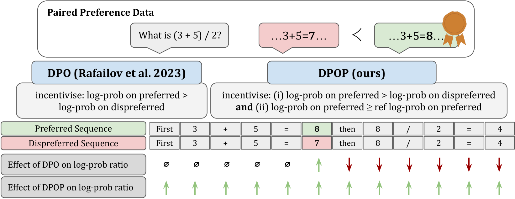
While the above illustrates a hypothetical situation, now we provide a specific case in which DPO may cause a decrease in the probability of the better completion. Consider the case of trying to improve a model’s math or reasoning abilities by comparing a completion of “2+2=4” to “2+2=5.” This process creates a pair of preferred and dispreferred completions which have an edit (Hamming) distance of 1, i.e., all tokens in the completion are the same except for one. In the following, we will explore how the location of the differing token impacts the computation of the DPO loss. For sake of argument, we will examine what happens when the differing token is the first token, though the argument also follows if it appears elsewhere.

For preliminaries, consider two completions with an edit distance of 1 which differ at token $m$ with $1\le m\le K$, i.e., consider $y_w=(t_1,\mathrm{\dots },t_K)$ and $y_l=(t_1,\mathrm{\dots },t_{m-1},t_m^{\prime },t_{m+1},\mathrm{\dots },t_K)$. Denote and $y^{\ge r}=(t_r,\mathrm{\dots },t_K)$. Assume that the vocabulary length of the LLM is $L$. Let $s_i^{\{x\}}$ represent the probability of the $i$-th token in the model’s vocabulary given the input $x$. While the LLM model parameters $\theta$ are numerous, we restrict our attention to the logits, ${\theta }_j$ with $j\in [L]$.

The gradient of Equation 1 with respect to $\theta$ is proportional to the following:

${\nabla }_{\theta }{ℒ}_{DPO}({\pi }_{\theta };{\pi }_{\text{ref}})\propto -\left[{\nabla }_{\theta }\log {\pi }_{\theta }(y_w|x)-{\nabla }_{\theta }\log {\pi }_{\theta }(y_l|x)\right].$

We note first that for $m>1$, all tokens from 1 to $m-1$ have no effect on the gradient, simply because for all , , causing these tokens’ contribution to the gradient to cancel out. Therefore, without loss of generality, assume $m=1$, i.e., $y_w$ and $y_l$ differ only at the first token. Without loss of generality, we also assume that $t_k$ takes vocabulary position 1. Then we have the following for each $k>1$ (derivation in Section B.1):

(2)

As we typically run DPO after SFT, the model is likely to be reasonably well optimised, so we should have for $j\ne 1$ and . Therefore, while this analysis only extends to gradients with respect to the logits, we see that the gradient vector is decreasing in the correct logit dimension and increasing in the wrong logit dimensions. Surprisingly, this suggests that under DPO, all tokens that follow a mismatched token should have reduced probability of emitting the correct token when compared to ${\pi }_{\text{ref}}$. We will later give empirical evidence for this in Section 5 and Figure 3.

4 DPOP

Now, we introduce DPO-Positive (DPOP), which is a solution to fix the failure mode described in the previous section. While there is no incentive for DPO to maintain the high log-likelihood of the preferred completions, DPOP adds the penalty term $\text{max}(0,\frac{\log {\pi }_{\text{ref}}(y_w|x)}{\log {\pi }_{\theta }(y_w|x)})$ to the loss. It is 0 when ${\pi }_{\text{ratio}}(y_w|x)\ge 1$ and increases as the ratio goes below 1. Thus, the DPOP loss function is:

${ℒ}_{\text{DPOP}}({\pi }_{\theta };{\pi }_{\text{ref}})=-{𝔼}_{(x,y_w,y_l)\sim D}[\log \sigma (\beta \log {\displaystyle \frac{{\pi }_{\theta }(y_w|x)}{{\pi }_{\text{ref}}(y_w|x)}}$ $-\beta \log {\displaystyle \frac{{\pi }_{\theta }(y_l|x)}{{\pi }_{\text{ref}}(y_l|x)}})$ (3)

$-\lambda \text{max}(0,\log {\displaystyle \frac{{\pi }_{\text{ref}}(y_w|x)}{{\pi }_{\theta }(y_w|x)}})]$

where $\lambda >0$ is a hyperparameter that can be tuned. This form of loss retains the property that we are fitting parameters on the preference data under the Bradley-Terry model. The implicit reward parameterisation is

$\beta \cdot {\displaystyle \frac{{\pi }_{\theta }(y|x)}{{\pi }_{\text{ref}}(y|x)}}\text{for}y=y_l,$ $\beta \left[\log {\displaystyle \frac{{\pi }_{\theta }(y_w|x)}{{\pi }_{\text{ref}}(y|x)}}-\lambda \text{max}(0,\log {\displaystyle \frac{{\pi }_{\text{ref}}(y|x)}{{\pi }_{\theta }(y|x)}})\right]\text{for}y=y_w.$

By applying this optimisation pressure, the model can no longer minimise the loss by significantly reducing the log-likelihood of the dispreferred examples more than it reduces the log-likelihood of the preferred examples; it must also ensure that the log-likelihood of the preferred examples remains high relative to the log-likelihood under the reference model.

Now, we show that Equation 3 mitigates our examples of failure modes from the previous section. Recall from Section 3 that we focused on two completions, $y_w$ and $y_l$, which differ by one token at location $m=1$. We showed in Equation 2 that for standard DPO, the gradient of the $k$-th token in the completions with respect to the $j$-th logit is . However, for DPOP, if , the gradients become

where $i$ is the vocabulary index of token $t_k$. Since , for the case $i=j$, the gradient is guaranteed to be positive for a large enough choice of $\lambda$. Similarly, for the case $i\ne j$, the gradient is guaranteed to be negative for a large enough $\lambda$ (as long as ). This therefore fixes the issue from Section 3. The derivation of the above is given in Section B.1.

Connection to Contrastive Loss

While the main motivation for DPOP is to avoid the failure mode described in Section 3, we also note its connection to contrastive loss. Contrastive learning is a popular technique in areas such as computer vision for datasets of similar and dissimilar pairs [Oord et al., 2018, Chen et al., 2020, He et al., 2020], and the loss function often uses a margin factor. Equation 3 can be viewed as similar to contrastive loss with margin $m=\log \frac{1}{{\pi }_{\text{ref}}(y_w|x)}$. We give further details in Appendix C.

5 DPOP Datasets & Experiments

In this section, we empirically validate that the failure mode does arise in practice and that DPOP is able to mitigate the failure. We also show that even when the edit distance is large and DPO does not show degradation in performance, DPOP can still outperform on downstream task evaluation.

5.1 Dataset Creation

For our empirical analysis, we focus on the downstream tasks of GSM8K, ARC, and HellaSwag, and we introduce and release associated paired preference-ranked datasets.

GSM8K [Cobbe et al., 2021], a dataset of diverse grade school math word problems, has been adopted as a measure of the math and reasoning skills of LLMs [Chowdhery et al., 2023, Touvron et al., 2023b, a, Beeching et al., 2023, Gao et al., 2021]. We create a paired preference-ranked version of MetaMath [Yu et al., 2023], an extended version of the GSM8K training data [An et al., 2023, Yu et al., 2023]. The correct completions in the MetaMath dataset consist of a series of steps which lead to the final answer. To create a dispreferred version, we randomly corrupt one of the results of an intermediate calculation. This dataset has a low (normalised) edit distance of 6.5%.

ARC [Clark et al., 2018] is a dataset that tests the level of understanding of science at grade-school level. We focus specifically on ARC-Challenge, the more difficult of the two subsections of ARC, which has been widely adopted as a measure of LLM reasoning and world understanding [Chowdhery et al., 2023, Touvron et al., 2023b, a, Beeching et al., 2023, Cobbe et al., 2021]. The ARC-Challenge dataset consists of four choices of responses to each question, one of which is correct. To create a paired preference-ranked dataset, for each correct response in the training split, we create three pairs using each incorrect response. Due to the differences in the responses, this dataset has a high normalised edit distance of 90%.

HellaSwag [Zellers et al., 2019] is a dataset containing commonsense inference questions known to be hard for LLMs. Similar to ARC, each question has one correct completion and three incorrect completions, and so we create a paired preference-ranked dataset by creating three pairs for each correct response in the training split. See Appendix D for further details and documentation about our newly released datasets.

Figure 2: DPOP vs. DPO vs. IPO. DPOP outperforms the other two methods on both MetaMath (left) whose normalized edit distance is 6.5%, and also ARC (right), whose normalized edit distance is 90%. Evaluation is performed on the test set of the datasets using the LLM Evaluation Harness.

5.2 Experiments

In this section, we compare training DPO, IPO, and DPOP on the datasets mentioned above and evaluate them on the corresponding tasks. We apply each preference-training method to the base model of Mistral7B [Jiang et al., 2023]. We evaluate on the test sets of GSM8K and ARC by using the LLM Evaluation Harness [Gao et al., 2021].

Loss function comparison

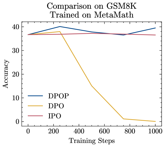
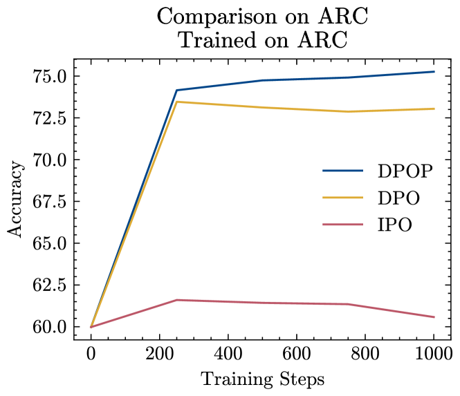
First, we compare DPO, IPO, and DPOP when training on both MetaMath and ARC; see Figure 2. We find that when training on MetaMath, DPO catastrophically fails, while IPO does not improve performance. DPOP is the only model to improve performance over the base model. When training on ARC, which has a higher edit distance as described in the previous section, both DPO and DPOP are able to improve on the base model significantly; however, DPOP performs better.

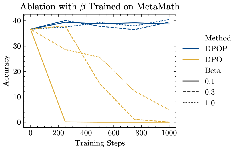
Ablation study over $\beta$

One potential hypothesis for how degradation of DPO on MetaMath could be prevented is by modifying the strength of the regularisation parameter, $\beta$. We test $\beta \in \{0.1,0.3,1.0\}$, and although a larger $\beta$ does induce a slower decrease, the performance with DPO still plummets, while DPOP shows strong and consistent performance with different values of $\beta$ (see Appendix Figure 4).

Token-level analysis

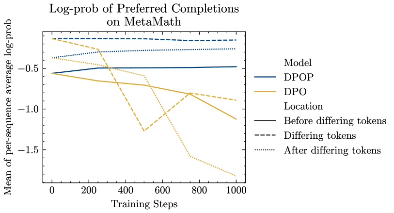
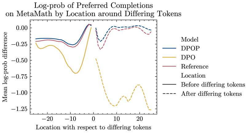
Recall that in Section 3, we gave theoretical motivations for why DPO is likely to perform poorly on low-edit distance datasets. We now analyse the log-probabilities of the trained models at the token level on the MetaMath dataset over 1000 samples to empirically support our arguments. Let us denote the index of the first token that is different between the preferred and dispreferred completion by $m$.

We suggested that for $r>m$ will have ‘wrong-way’ gradient updates and therefore decrease. We find this is indeed the case—the average log-prob after training of tokens after $m$ is $-0.37$ for the reference model and $-0.26$ for DPOP, but $-1.82$ for DPO on the preferred completions (see (Figure 3) (left)). Perhaps most instructively, for both the reference model and DPOP, in Figure 3 (right), we see that tokens after the edit indices show higher log-likelihood than those before the edit indices—this is indicative of well-behaved language modelling, with lower perplexity as more tokens are added to the context. By contrast, DPO shows the opposite pattern—with log-likelihood actually reducing after the edit indices. This is indicative of a deeper breakdown in language modelling, which we believe is facilitated by the wrong-way gradient we outlined in Section 3. Finally, we are also able to substantiate our assumption from Section 3 that $s_1\ge s_1^{\prime }$; we find from our analysis that for the baseline model, the tokens after the edit have an average log-likelihood of $-0.37$ on the preferred completion, but this drops to $-0.86$ on the dispreferred completion.

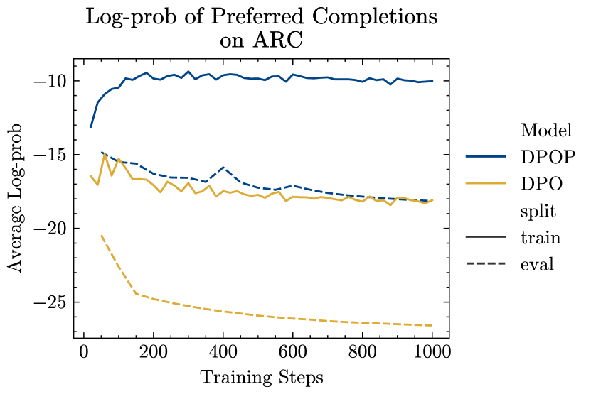
In Appendix E, we present additional results on ARC comparing the averaged log-probs of DPO and DPOP on the preferred completion during training; see Figure 6. DPOP once again demonstrates higher log-probs than DPO.

Figure 3: DPO fails to train on low edit-distance pairs, yet DPOP performs well. Left: average log-probs for 912 randomly-sampled preferred train set completions on MetaMath across training steps. For DPO, the log-probs decrease as training progresses. Right: average log-prob difference for preferred completions on MetaMath by location around differing tokens, after 1000 training steps. Log-prob ‘difference’ signifies that each model’s plot has been adjusted to have 0 log-prob at location -1; all other log-probs are shown relative to this value to emphasise relative trends at different points in the sequence. For DPO, there is a significant decrease after the differing tokens, while DPOP avoids this issue.

6 Smaug

In this section, we introduce the Smaug series of models. We train models for 7B, 34B and 72B parameter sizes using DPOP. We use the 7B class for a direct comparison of DPOP vs. DPO, including on existing and widely-used paired preferenced-ranked datasets. Due to the computational resource requirements involved in training the larger model sizes, we only perform DPOP on 34B and 72B and compare to other models on the HuggingFace Open LLM Leaderboard. For the same reason, we also do not perform any hyperparameter tuning; it is possible that even better performance can be achieved, e.g., with a different value of $\lambda$.

6.1 Smaug-34B and Smaug-72B

Table 1: Evaluation of the top open-weight models on the HuggingFace Open LLM Leaderboard as of February 1st, 2024. See Table 3 for an extended comparison.

Model	Size	Avg.	ARC	HellaSwag	MMLU	TruthfulQA	Winogrande	GSM8K
Smaug-72B (Ours)	72B+	80.48	76.02	89.27	77.15	76.67	85.08	78.70
MoMo-72B-lora-1.8.7-DPO	72B+	78.55	70.82	85.96	77.13	74.71	84.06	78.62
TomGrc_FusionNet_34Bx2_MoE_v0.1_DPO_f16	72B+	77.91	74.06	86.74	76.65	72.24	83.35	74.45
TomGrc_FusionNet_34Bx2_MoE_v0.1_full_linear_DPO	72B+	77.52	74.06	86.67	76.69	71.32	83.43	72.93
Truthful_DPO_TomGrc_FusionNet_7Bx2_MoE_13B	72B+	77.44	74.91	89.30	64.67	78.02	88.24	69.52

Smaug-34B is a modified version of the base model Bagel-34B-v0.2 [Durbin, 2024a], which itself is a SFT version of Yi-34B-200k [01.AI, 2024]. We first take Bagel-34B-v0.2 and perform a SFT fine-tune using a combination of three datasets: MetaMath [Yu et al., 2023], ORCA-Chat [Es, 2024], and the ShareGPT dataset [Z., 2024]. Next, we perform DPOP with five datasets: our pairwise MetaMath DPO, ARC DPO, and HellaSwag DPO datasets described in Section 5, the ORCA DPO dataset [Intel, 2024], and the UltraFeedback Binarized dataset [AllenAI, 2024]. Finally, we perform a standard DPO with the Truthy DPO dataset [Durbin, 2024b]. We run these experiments with 8 H100 GPUs. We set $\beta =0.3$, $\lambda =50$, a learning rate of $5\times {10}^{-5}$, and the AdamW optimizer [Loshchilov and Hutter, 2017], and we run 1000 steps for all DPOP routines. The total training time for all steps took 108 hours.

For 72B, we start from MoMo-72b-lora-1.8.7-DPO [Moreh, 2024], which itself is a fine-tune of Qwen-72B [Bai et al., 2023]. MoMo-72b-lora-1.8.7-DPO has already undergone SFT, so we simply run the five DPOP routines as in Smaug-34B. The total training time is 144 hours.

HuggingFace Open LLM Leaderboard

We evaluate using the HuggingFace Open LLM Leaderboard [Beeching et al., 2023, Gao et al., 2021], a widely-used benchmark suite that aggregates six popular benchmarks: ARC [Clark et al., 2018], GSM8K [Cobbe et al., 2021], HellaSwag [Zellers et al., 2019], MMLU [Hendrycks et al., 2021], TruthfulQA [Lin et al., 2022], and WinoGrande [Sakaguchi et al., 2020]. We evaluate directly in HuggingFace, which uses the LLM Evaluation Harness [Gao et al., 2021]. It performs few-shot prompting on the test sets of these tasks and checks if the model emits the correct answer. We compare Smaug-72B to the evaluation scores of the top five open-weight LLMs according to the HuggingFace Open LLM Leaderboard [Beeching et al., 2023, Gao et al., 2021] as of February 1, 2024; see Table 1. Smaug-72B achieves an average accuracy of 80.48%, becoming the first open-source LLM to surpass an average accuracy of 80% and improving by nearly 2% over the second-best open-source model. Smaug-34B also achieves best-in-its-class performance compared to other models of similar or smaller size (see Appendix E).

MT-Bench

Next, we evaluate using MT-Bench [Zheng et al., 2023], a challenging benchmark that uses GPT-4 [OpenAI, 2023] to score candidate model responses across eight different categories of performance. As shown in other works [Zheng et al., 2023, Rafailov et al., 2023], strong LLMs such as GPT-4 show good agreement with human preferences. We run MT-Bench with the Llama-2 conversation template [Touvron et al., 2023b]. See Table 2 for a comparison with state-of-the-art LLMs according to Arena Elo as of February 1, 2024. Smaug-72B achieves the top MMLU score and third-best MT-bench score out of the open-source models in Table 2. In Appendix E, we give examples of Smaug-72B completions to MT-Bench questions.

Table 2: Evaluation of the top models according to Elo, MT-Bench, and MMLU.

Model	Arena Elo	MT-bench	MMLU	Organization	License
GPT-4-1290-preview	1253			OpenAI	Proprietary
GPT-4-1106-preview	1252	9.32		OpenAI	Proprietary
Bard (Gemini Pro)	1224			Google	Proprietary
GPT-4-0314	1190	8.96	86.4	OpenAI	Proprietary
GPT-4-0613	1162	9.18		OpenAI	Proprietary
Mistral Medium	1150	8.61	75.3	Mistral	Proprietary
Claude-1	1149	7.9	77	Anthropic	Proprietary
Claude-2.0	1132	8.06	78.5	Anthropic	Proprietary
Gemini Pro (Dev API)	1120		71.8	Google	Proprietary
Claude-2.1	1119	8.18		Anthropic	Proprietary
GPT-3.5-Turbo-0613	1118	8.39		OpenAI	Proprietary
Mixtral-8x7b-Instruct-v0.1	1118	8.3	70.6	Mistral	Apache 2.0
Yi-34B-Chat	1115		73.5	01 AI	Yi License
Gemini Pro	1114		71.8	Google	Proprietary
Claude-Instant-1	1109	7.85	73.4	Anthropic	Proprietary
GPT-3.5-Turbo-0314	1105	7.94	70	OpenAI	Proprietary
WizardLM-70B-v1.0	1105	7.71	63.7	Microsoft	Llama 2 Community
Tulu-2-DPO-70B	1104	7.89		AllenAI/UW	AI2 ImpACT Low-risk
Vicuna-33B	1093	7.12	59.2	LMSYS	Non-commercial
Starling-LM-7B-alpha	1090	8.09	63.9	UC Berkeley	CC-BY-NC-4.0
Smaug-72B		7.76	77.15	Abacus.AI	tongyi-qianwen-license-agreement

6.2 Comparison using 7B Model

We fine-tune Smaug-7B from a base of Llama 2-chat [Touvron et al., 2023b]. Since Llama 2-chat has already undergone instruction fine-tuning, we perform DPO and DPOP directly using the same datasets described in the previous section. We train for 2 000 steps on 1xGH200.

MT-Bench

We evaluate Smaug-7B on MT-Bench in the same setting as described in the previous section. We find that DPOP achieves a first-turn score of 7.275 whereas DPO achieves a score of 7.076.

7 Conclusion, Limitations, and Impact

In this work, we presented new theoretical and empirical findings on a severe failure mode of DPO, in which fine-tuning causes the probability of the preferred examples to be reduced. In order to mitigate this issue, we devised a new technique, DPOP, which we show overcomes the failure mode of DPO—and can outperform DPO even outside this failure mode. By fine tuning with DPOP on our new pairwise preference versions of ARC, HellaSwag, and MetaMath, we create a new LLM that achieves state-of-the-art performance. In particular, it is the first open-weights model to surpass an average accuracy of 80% on the HuggingFace Open LLM Leaderboard, and it is nearly 2% better than any prior open-weight LLM.

In the future, creating pairwise preference-based versions of other datasets, and running DPOP with these datasets, could push the abilities of open-source LLMs even closer to the performance of proprietary models such as GPT-4 [OpenAI, 2023]. Furthermore, using DPOP on additional mathematical datasets is an exciting area for future work, as it has the potential to further advance LLMs’ abilites in mathematial reasoning.

Limitations

While our work gives theoretical and empirical evidence on a failure mode of DPO and a proposed solution, it still has limitations. First, we were unable to run a full ablation study on our 72B model. Running multiple fine-tuning experiments on a 72B model is infeasible, as each one can take over five days to complete. Therefore, we assume that our ablations on smaller models still hold up at scale. Furthermore, while we expect DPOP to achieve strong performance on any preference dataset, especially those with small edit distance, we have only demonstrated its performance on five English-language datasets. We hope that future work can verify its effectiveness on more datasets, in particular on non-English datasets.

Broader Impact

This paper proposes a technique to fine-tune LLMs using preference data, releases three preference datasets based on mathematics and reasoning, and releases new LLMs fine-tuned on the preference data. As with any paper that releases a fine-tuning technique or an LLM, there are inherent risks. An adversary could use such a technique to create a model fine-tuned to produce harmful, toxic, or illegal content. However, we are optimistic that our work will have a net positive impact. In particular, DPOP is especially beneficial when used with mathematical or reasoning datasets, in which only a few tokens differ between the preferred and less-preferred completions. Furthermore, we give theoretical intuition on the failure cases of DPO, and a method to avoid this failure case, therefore moving towards a more complete understanding of preference optimisation-based techniques. With recent extensive efforts towards AI safety [Huang et al., 2023, Yao et al., 2023, Weidinger et al., 2021], we hope that preference optimisation-based techniques will impact society positively. Finally, we note that the models we release are less performant than the current top proprietary models such as GPT-4 [OpenAI, 2023], therefore lessening the negative impact of releasing our models.

Appendix A Related Work Continued

In this section, we continue our discussion of related work from Section 2.

AFT

Wang et al. [2023] seek to align LLMs to correctly ‘score’ (in terms of perplexity) their own generations. They do so by generating multiple chain-of-thought [Wei et al., 2023] responses to each prompt, which they categorise as preferred or dispreferred according to whether they answer the question correctly. Their proposed ‘Alignment Fine-Tuning (AFT)’ paradigm adds an alignment objective ${ℒ}_A^{*}$ to the standard fine tuning loss, defined as

${ℒ}_A^{*}({\pi }_{\theta })=\log \left[1+{\displaystyle \sum _{y_w\in {𝒢}_W}}{\displaystyle \sum _{y_l\in {𝒢}_L}}{e}^{(\log {\pi }_{\theta }(y_l|x)-\log {\pi }_{\theta }(y_w|x))}\right]$

where ${𝒢}_p$ is the set of preferred examples and ${𝒢}_n$ is the set of dispreferred examples. By minimising ${ℒ}_A^{*}$, the log-likelihoods of preferred examples are encouraged to be larger than the log-likelihoods of dispreferred examples, akin to DPO. However, Wang et al. [2023] takes an opposing motivation to us: they are particularly concerned with the issue of the log-likelihoods of dispreferred examples being pushed down too significantly

Our work differs from AFT in three key points. First, although Wang et al. [2023] discusses DPO in the appendix, they do not show how their approach would extend to a reformulation of its objective; they also focus their experiments solely on supervised fine-tuning. Next, we use a different constraint mechanism—theirs is a soft margin constraint on the log-probability distance of the dispreferred example from the preferred example, while ours is a soft penalty for deviating from a reference model. Finally, they are focused specifically on the case of self-generated LLM CoT responses and calibrating the LLM’s perplexity of its own responses.

HALO

Ethayarajh et al. [2023] seek to understand alignment methods, including DPO, in the context of ‘Human-Centred Loss Functions (HALOs)’. By drawing an equivalence between the alignment methods and the work of Tversky and Kahneman [1992] in prospect theory, they adapt the ‘human value function’ in that paper to the LLM setting:

$$L_{KTO}({\pi }_{\theta },{\pi }_{\text{ref}})={𝔼}_{x,y\sim D}\left[w(y)(1-\widehat{h}(x,y;\beta ))\right]$$

where they define $g(x,y;\beta )$ as

$$\beta \log \frac{{\pi }_{\theta }(y|x)}{{\pi }_{\text{ref}}(y|x)}-{𝔼}_{x^{\prime }\sim D}\left[\beta \text{KL}({\pi }_{\theta }||{\pi }_{\text{ref}})\right]$$

and

$h(x,y;\beta )$

$w(y)$

The major difference of this approach with DPO is that it does not require paired preference data. The above loss function can be used for any dataset as long as the labels are individually marked as positive or negative.

CPO

Very recently, concurrent work [Xu et al., 2024] proposes adding a new term to the DPO loss function in order to allow DPO to become better at rejecting ‘worse’ completions that are good quality but not perfect. Specifically, they include the term

$${𝔼}_{(x,y_w,y_l)\sim D}\left[\log {\pi }_{\theta }(y_w\mid x)\right].$$

While similar, their work uses a different loss function with different motivation, and furthermore they only considered machine translation models up to 13B parameters.

Appendix B Derivation of logit gradients

B.1 Derivation for DPO

Consider two completions of length $K$ with edit (Hamming) distance of 1 which differ at token $m$ with $1\le m\le K$. Put $y_w=(t_1,\mathrm{\dots },t_K)$ and $y_l=(t_1,\mathrm{\dots },t_{m-1},t_m^{\prime },t_{m+1},\mathrm{\dots },t_K)$. Put and $y^{\ge r}=(t_r,\mathrm{\dots },t_K)$. Note that the derivative of Equation 1 with respect to $\theta$ is proportional to:

${\nabla }_{\theta }{ℒ}_{DPO}({\pi }_{\theta };{\pi }_{\text{ref}})\propto -\left[{\nabla }_{\theta }\log {\pi }_{\theta }(y_w|x)-{\nabla }_{\theta }\log {\pi }_{\theta }(y_l|x)\right]$

By the chain rule, we have

and by using logarithm identities

When we substitute this into ${\nabla }_{\theta }{ℒ}_{DPO}$, we observe

${\nabla }_{\theta }{ℒ}_{DPO}({\pi }_{\theta };{\pi }_{\text{ref}})\propto$

Assume that the vocabulary length of the LLM is $L$. This means that ${\pi }_{\theta }(y|x)$ corresponds to a vector of length $L$ and represents the softmax output of the final layer of the LLM, i.e., ${𝒔}^{\mathbf{\{}𝒙\mathbf{\}}}={\pi }_{\theta }(y|x)$. Note, we may drop the $x$ from the notation of $𝒔$ if the context is obvious. Therefore, $s_i^{\{x\}}$ represents the probability of the $i$-th token in the model’s vocabulary given the input context $x$.

While the LLM model parameters $\theta$ are numerous, let us restrict our attention to just the logits, which we denote as ${\theta }_j$ with $j\in [L]$ and are the input to the softmax. With this assumption, we know that

${\displaystyle \frac{\partial }{\partial {\theta }_j}}\log s_i^{\{x\}}=1\{i=j\}-s_j^{\{x\}}.$ (4)

Consider the case where $y_w$ and $y_l$ differ only at the first token, i.e., $m=1$. In this instance, we have that for $k>1$:

Without loss of generality, assume that $t_k$ takes vocabulary position 1. Then from Equation 4, we have:

(5)

As we typically run DPO after SFT the model is likely to be reasonably well optimised, so we should have for $j\ne 1$ and . Therefore, while this analysis only extends to gradients with respect to the logits, we see that the gradient vector is decreasing in the correct logit dimension and increasing in the wrong logit dimensions. In particular, this derivation suggests that under DPO, all tokens that follow a difference at $m$ at any point should have reduced probability of emitting the correct token when compared to ${\pi }_{\text{ref}}$.

B.2 Derivation for DPOP

We can follow a similar line of reasoning for calculating ${\nabla }_{\theta }{ℒ}_{DPOP}$ with respect to its logits which we denote again by ${\theta }_j$.

Again taking token position $t_k$ for illustrative purposes and assuming that $t_k$ takes vocabulary position $i$, in the case when ,

In the case when ${\pi }_{\text{ratio}}(y|x)\ge 1$, then we have the standard gradient from ${ℒ}_{\text{DPO}}$.

Appendix C Motivation: Contrastive Loss

While the main motivation for DPOP is to avoid the failure mode described in Section 3, we also note its connection to contrastive loss. Contrastive learning is widely used [Wang and Liu, 2021, Wang and Isola, 2020, Saunshi et al., 2019, Oord et al., 2018, Chen et al., 2020, He et al., 2020], often for embedding learning applications. The contrastive loss formulation typically includes two main terms: one encouraging the proximity of analogous inputs, the other encouraging the divergence of distinct classifiable data.

Moreover, the introduction of a margin appended to one of these terms often ensures a more stable training process. This margin serves as an indicator of indifference to point displacement once a specific value threshold is exceeded. The margin, when attached to the similar points term, establishes a minimum threshold beyond which we do not care about pulling the points closer. Alternatively, if added on the dissimilar points term, the margin sets a maximum threshold.

We show that the DPO loss is structured such that learning the probabilities during DPO training are equivalent to learning the embeddings in a contrastive loss formulation. However, the standard DPO only uses the term computing distance between dissimilar points, and does not include the similar points term or the margin. Consequently, it is predictable that traditional DPO’s inefficiencies mirror the known shortcomings of contrastive training when one constituent term is absent. DPOP, our refined DPO formulation, fixes this by adding the absent term and the margin.

Contrastive loss is defined in Hadsell et al. [2006]. If we keep the margin in the similar points terms, it can be written as follows:

${ℒ}_{\text{Cont}}=$ $-{\displaystyle \sum _{\forall (i,j)ϵ{𝒫}_d}}𝒟(y_i,y_j)+\lambda {\displaystyle \sum _{\forall (i,j)ϵ{𝒫}_s}}\min (𝒟(y_i,y_j)-m,0)$

Recall that the standard DPO loss (Equation 1) is as follows:

${ℒ}_{\text{DPO}}({\pi }_{\theta };{\pi }_{\text{ref}})=-{𝔼}_{(x,y_w,y_l)\sim D}\left[\log \sigma \left(\beta \log {\displaystyle \frac{{\pi }_{\theta }(y_w|x)}{{\pi }_{\text{ref}}(y_w|x)}}-\beta \log {\displaystyle \frac{{\pi }_{\theta }(y_l|x)}{{\pi }_{\text{ref}}(y_l|x)}}\right)\right]$

Say we designate an embedding function $\mathscr{H}$:

$\mathscr{H}(y|x)={\displaystyle \frac{{\pi }_{\theta }(y|x)}{{\pi }_{\text{ref}}(y|x)}}.$

And we define a distance function $𝒟$ as follows:

$𝒟(p_i,p_j)=\log [\mathscr{H}(p_i)]-\log [\mathscr{H}(p_j)].$

The standard DPO only has the dissimilar points term under the analogy of the contrastive loss formulation. For more robust training we accommodate for the similar embeddings term. We use the concept of anchor points or embeddings for both positive and negative points as in triplet loss Schroff et al. [2015]. These points are known ideal embeddings we want our points to achieve. They carry probabilities of 1 and 0 respectively in our equivalence depending on whether they are preferred or dispreferred samples.

${\mathscr{H}}_p^{*}(y|x)$ $={\displaystyle \frac{1}{{\pi }_{\text{ref}}(y|x)}}$

${\mathscr{H}}_n^{*}(y|x)$ $={{\displaystyle \frac{ϵ}{{\pi }_{\text{ref}}(y|x)}}|}_{ϵ\to 0}$

The DPOP loss can thus be formulated as:

${ℒ}_{\text{DPOP}}$ $=[\log (\mathscr{H}(y_w|x))-\log (\mathscr{H}(y_l|x))]+\lambda [\min (\log ({\mathscr{H}}_p^{*}(y_w|x))-\log (\mathscr{H}(y_w|x))-m,0)$

$+\min (\log ({\mathscr{H}}_n^{*}(y_l|x))-\log (\mathscr{H}(y_l|x))-m,0)]$

$=\left[\log {\displaystyle \frac{{\pi }_{\theta }(y_w|x)}{{\pi }_{\text{ref}}(y_w|x)}}-\log {\displaystyle \frac{{\pi }_{\theta }(y_l|x)}{{\pi }_{\text{ref}}(y_l|x)}}\right]+\lambda \left[\min (\log {\displaystyle \frac{1}{{\pi }_{\text{ref}}(y_w|x)}}-\log {\displaystyle \frac{{\pi }_{\theta }(y_w|x)}{{\pi }_{\text{ref}}(y_w|x)}}-m,0)\right]$

$+\lambda \left[\min (\log {\displaystyle \frac{ϵ}{{\pi }_{\text{ref}}(y_l|x)}}-\log {\displaystyle \frac{{\pi }_{\theta }(y_l|x)}{{\pi }_{\text{ref}}(y_l|x)}}-m,0)\right]$

If we set the margin $m=\log \frac{1}{{\pi }_{\text{ref}}(y_w|x)}$, the second term is:

$=-\lambda \left[\max (\log {\displaystyle \frac{{\pi }_{\theta }(y_w|x)}{{\pi }_{\text{ref}}(y_w|x)}},0)\right]$

This choice of margin is mathematically equivalent to choosing a threshold which ensures the similarity term only contributes to the loss when the learned model performs worse on the preferred response than the base model.

We can ignore the third term during training for two primary reasons. First, it is trying to push the log probability of negative samples to negative infinity which may be unstable during training. Second, in essence, it negatively impacts the likelihood of the negative samples. However, given our objective of extending the distance between positive and negative samples without diminishing the likelihood of positives, sacrificing this signal is acceptable. In the worst-case scenario, while the probability of negatives may be increased, the consequent increase in the probability of positives is ensured by the first two terms, thus rendering the sacrifice acceptable.

Appendix D Details of Datasets

In this section, we give more details and examples of the three datasets we release. We release all datasets under the Apache 2.0 License.

MetaMath

GSM8K [Cobbe et al., 2021] is a dataset of diverse grade school maths word problems, which has been commonly adopted as a measure of the math and reasoning skills of LLMs [Chowdhery et al., 2023, Touvron et al., 2023b, a, Beeching et al., 2023, Gao et al., 2021]. The MetaMath dataset is partitioned into queries and responses, where the query is a question involving mathematical calculation or reasoning, and the response is a logical series of steps and calculations that culminate in a final answer. To construct our paired-preference version of MetaMath, we take the queries as prompts $x$ and the responses as the preferred completions $y_w$. We create $y_l$ by modifying the response by randomly corrupting one of the results of an intermediate calculation so that it is incorrect; however, we leave the answer untouched.

An example is as follows: $x$: “What is the total cost of purchasing equipment for all sixteen players on the football team, considering that each player requires a $25 jersey, a $15.20 pair of shorts, and a pair of socks priced at $6.80?" $y_w$: “Each player requires a $25 jersey, a $15.20 pair of shorts, and a pair of socks priced at $6.80. So the total cost for each player is $25 + $15.20 + $6.80 = $47. Since there are sixteen players on the football team, the total cost for all of them is 16 * $47 = $752. #### 752 The answer is: 752" $y_l$: “Each player requires a $25 jersey, a $15.20 pair of shorts, and a pair of socks priced at $6.80. So the total cost for each player is $25 + $15.20 + $6.80 = $52. Since there are sixteen players on the football team, the total cost for all of them is 16 * $47 = $752. #### 752 The answer is: 752"

The dataset contains 393 999 training examples and 1 000 evaluation examples. Our motivation in building this dataset is to align models towards being precise in intermediate calculations. This dataset has low edit distance – the normalised edit distance is approximately 6.5%.

ARC

ARC [Clark et al., 2018] is a dataset that tests the level of understanding of science at approximately grade-school level. We focus specifically on the ‘Challenge’ subsection of ARC, the more difficult of the two subsections, which has been widely adopted as a measure of LLM reasoning and world understanding [Chowdhery et al., 2023, Touvron et al., 2023b, a, Beeching et al., 2023, Gao et al., 2021, Cobbe et al., 2021]. We create a paired preference-ranked dataset from the train split of ARC-Challenge. The dataset is partitioned into questions which we take as our prompts $x$, and four choices of responses to each question of which only one is the correct answer. The correct response is taken as $y_w$ and the incorrect responses are taken to be $y_l$; as there are three incorrect responses for every prompt, we repeat $y_w$ multiple times for each prompt. The dataset contains 3357 training examples and 895 evaluation examples. This dataset has a high normalised edit distance of approximately 90%.

HellaSwag

Finally, we consider the HellaSwag dataset [Zellers et al., 2019], a dataset containing commonsense inference questions known to be hard for LLMs. An example prompt is “Then, the man writes over the snow covering the window of a car, and a woman wearing winter clothes smiles. then” And the potential completions are $[$ ", the man adds wax to the windshield and cuts it.", ", a person board a ski lift, while two men supporting the head of the person wearing winter clothes snow as the we girls sled.", ", the man puts on a christmas coat, knitted with netting.", ", the man continues removing the snow on his car." $]$ The dataset contains 119 715 training and 30 126 evaluation examples.

Appendix E Additional Experiments and Details

E.1 Additional Training Details

No hyperparameter tuning was done when creating Smaug-34B or Smaug-72B. DPOP has two hyperparameters, $\beta$ and $\lambda$. We chose $\beta =0.3$, similar to prior work [Rafailov et al., 2023], and we chose $\lambda =50$ without trying other values. It is possible that even better performance can be achieved, e.g., with a different value of $\lambda$.

Here, we give the licenses of all models used to train our Smaug-series of models.

Smaug-7B started from Llama 2-chat [Touvron et al., 2023b]. Therefore, we release it under the Llama 2 license (https://ai.meta.com/llama/license/).

Smaug-34B started from Bagel-34B-v0.2 [Durbin, 2024a], which itself is a SFT version of Yi-34B-200k [01.AI, 2024]. Therefore, we release Smaug-34B under the Yi Series Models Community License Agreement (https://github.com/01-ai/Yi/blob/main/MODEL_LICENSE_AGREEMENT.txt).

Smaug-72B started from MoMo-72b-lora-1.8.7-DPO [Moreh, 2024], which itself is a fine-tune of Qwen-72B [Bai et al., 2023]. Therefore, we release Smaug-72B under the Qwen license (https://github.com/QwenLM/Qwen/blob/main/Tongyi%20Qianwen%20LICENSE%20AGREEMENT).

E.2 Additional Results

Ablation study for $\beta$

In Section 5, we described an ablation study on $\beta$ to reject one potential hypothesis for how degradation of DPO on MetaMath could be prevented is by modifying the strength of $\beta$, the regularisation parameter. Here, we present the plot; see Figure 4. We test $\beta \in \{0.1,0.3,1.0\}$. Although a larger $\beta$ does induce a slower decrease, the performance with DPO still plummets. On the other hand, DPOP shows strong and consistent performance with different values of $\beta$.

Figure 4: Evaluation of DPO vs. DPOP for different values of $\beta$, on the MetaMath dataset.

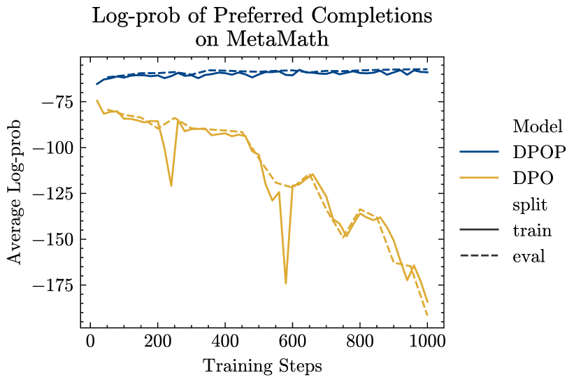
Log-probabilities of preferred completions

In Figure 5, we show the log-probabilities of the preferred completion of the train and eval sets during training on MetaMath. We plot the log-probabilities in more granularity than in Figure 3. We confirm our theoretical insights from Section 4 – the log-probabilities of the preferred completion drop substantially in DPO, whereas they increase for DPOP – across both the train and eval sets. For ARC, we see in Figure 6 that DPOP maintains high train-set log-probs, while both the train and eval set log-probs decrease for DPO. Notably, even though eval set log-probs do decrease for DPOP, they are still higher than the train set log-probs of DPO.

Figure 5: Average log-probs for preferred completions of DPOP and DPO on the MetaMath dataset showing the failure mode of DPO.

Figure 6: Average log-probs for preferred completions of DPOP and DPO on the ARC dataset showing the failure mode of DPO.

Additional tables

In Table 3, we give an extension of Table 1 (whose experimental details are in Section 6). In Table 4, we give the same table, except for models of size 34B or lower.

Table 3: (Extension of Table 1.) Evaluation of the top open-weight models on the HuggingFace Open LLM Leaderboard as of February 1st, 2024. Our 72B model achieves an average accuracy of 80.48%, becoming the first open-source LLM to surpass an average accuracy of 80% and improving by nearly 2% over the second-best open-source model (other than a fine-tune of our own model).

Model	Avg.	ARC	HellaSwag	MMLU	TruthfulQA	Winogrande	GSM8K
Smaug-72B (Ours)	80.48	76.02	89.27	77.15	76.67	85.08	78.70
MoMo-72B-lora-1.8.7-DPO	78.55	70.82	85.96	77.13	74.71	84.06	78.62
TomGrc_FusionNet_34Bx2_MoE_v0.1_DPO_f16	77.91	74.06	86.74	76.65	72.24	83.35	74.45
TomGrc_FusionNet_34Bx2_MoE_v0.1_full_linear_DPO	77.52	74.06	86.67	76.69	71.32	83.43	72.93
Truthful_DPO_TomGrc_FusionNet_7Bx2_MoE_13B	77.44	74.91	89.30	64.67	78.02	88.24	69.52
CCK_Asura_v1	77.43	73.89	89.07	75.44	71.75	86.35	68.08
FusionNet_34Bx2_MoE_v0.1	77.38	73.72	86.46	76.72	71.01	83.35	73.01
MoMo-72B-lora-1.8.6-DPO	77.29	70.14	86.03	77.40	69.00	84.37	76.80
Smaug-34B-v0.1 (Ours)	77.29	74.23	86.76	76.66	70.22	83.66	72.18
Truthful_DPO_TomGrc_FusionNet_34Bx2_MoE	77.28	72.87	86.52	76.96	73.28	83.19	70.89
DARE_TIES_13B	77.10	74.32	89.5	64.47	78.66	88.08	67.55
13B_MATH_DPO	77.08	74.66	89.51	64.53	78.63	88.08	67.10
FusionNet_34Bx2_MoE	77.07	72.95	86.22	77.05	71.31	83.98	70.89
MoE_13B_DPO	77.05	74.32	89.39	64.48	78.47	88.00	67.63
4bit_quant_TomGrc_FusionNet_34Bx2_MoE_v0.1_DPO	76.95	73.21	86.11	75.44	72.78	82.95	71.19
MixTAO-7Bx2-MoE-Instruct-v7.0	76.55	74.23	89.37	64.54	74.26	87.77	69.14
Truthful_DPO_cloudyu_Mixtral_34Bx2_MoE_60B0	76.48	71.25	85.24	77.28	66.74	84.29	74.07
MoMo-72B-lora-1.8.4-DPO	76.23	69.62	85.35	77.33	64.64	84.14	76.27
FusionNet_7Bx2_MoE_v0.1	76.16	74.06	88.90	65.00	71.20	87.53	70.28
MBX-7B-v3-DPO	76.13	73.55	89.11	64.91	74.00	85.56	69.67

Table 4: Evaluation of the top open-weight models on the HuggingFace Open LLM Leaderboard for models less than 35B parameters as of February 1st, 2024. Our 34B model achieves best-in-its-class performance compared to other models of similar or smaller size.

Model	Size	Avg.	ARC	HellaSwag	MMLU	TruthfulQA	Winogrande	GSM8K
Smaug-34B-v0.1 (Ours)	<35B	77.29	74.23	86.76	76.66	70.22	83.66	72.18
DARE_TIES_13B	<35B	77.10	74.32	89.50	64.47	78.66	88.08	67.55
13B_MATH_DPO	<35B	77.08	74.66	89.51	64.53	78.63	88.08	67.10
MoE_13B_DPO	<35B	77.05	74.32	89.39	64.48	78.47	88.00	67.63
4bit_quant_TomGrc_FusionNet_34Bx2_MoE_v0.1_DPO	<35B	76.95	73.21	86.11	75.44	72.78	82.95	71.19

Appendix F Example Completions

In this section, we give example completions by Smaug-72B for questions in MT-Bench [Zheng et al., 2023]. Note that these are not cherry-picked – they include examples of both good and bad completions.

Example 1

Question: Imagine you are writing a blog post comparing two popular smartphone models. Develop an outline for the blog post, including key points and subheadings to effectively compare and contrast the features, performance, and user experience of the two models. Please answer in fewer than 200 words.

Outline: 1. Introduction to the two smartphone models being compared (mention brand names and models) 2. Design and Build Quality • Comparison of dimensions, weight, materials used, and overall aesthetic appeal • Water and dust resistance, if applicable 3. Display and Screen Quality • Comparison of screen technology (OLED, IPS LCD, etc.) • Display resolution, refresh rate, and brightness levels 4. Performance and Hardware • Processor, RAM, and storage configurations • Comparison of benchmark scores (e.g., AnTuTu, Geekbench) 5. Camera System and Image Quality • Comparison of primary, ultra-wide, telephoto, and macro lenses (if available) • Comparison of low-light performance and image processing capabilities 6. Battery Life and Charging • Battery capacity and estimated usage time • Charging technologies (wired, wireless, fast charging, reverse charging) 7. Software and User Experience • Comparison of operating systems (iOS vs. Android) and their features • User interface, customization options, and app ecosystem 8. Additional Features and Extras • Comparison of biometric authentication (fingerprint, face unlock, etc.) • Additional features like NFC, 5G connectivity, and audio quality 9. Pricing and Value for Money • Comparison of retail prices and current offers • Assessment of overall value considering the features and performance 10. Conclusion and recommendation for potential buyers based on their preferences

Example 2

Question: In a survey conducted at a local high school, preferences for a new school color were measured: 58% of students liked the color blue, 45% preferred green, and 22% liked both colors. If we randomly pick a student from the school, what’s the probability that they would like neither blue nor green?

To find the probability that a randomly picked student would like neither blue nor green, we need to find the percentage of students who like only one color or neither color. From the given information, we know: • 58% like blue • 45% prefer green • 22% like both colors To find the percentage of students who like only one color, we can subtract the percentage of students who like both colors from the sum of students who like blue and green: • 58% (blue) + 45% (green) - 22% (both) = 83% Now, to find the probability of a student liking neither blue nor green, we subtract the percentage of students who like at least one color from 100%: • 100% - 83% = 17% So, the probability that a randomly picked student would like neither blue nor green is 17%.

Example 3

Question: Implement a program to find the common elements in two arrays without using any extra data structures.

Finding common elements in two arrays without using extra data structures can be achieved by using a simple algorithm. Here’s a Python implementation of this problem: ⬇ def find_common_elements(arr1, arr2): common_elements = [] for num1 in arr1: if num1 in arr2 and num1 not in common_elements: common_elements.append(num1) return common_elements # Example usage: array1 = [1, 2, 3, 4, 5] array2 = [4, 5, 6, 7, 8] print(find_common_elements(array1, array2)) # Output: [4, 5] This program iterates through the elements of the first array (arr1) and checks if each element is present in the second array (arr2). If it is, and the element hasn’t been added to the common_elements list yet, it is appended. The function then returns the list of common elements.

Example 4

Question: Identify the named entities (people, organizations, locations) mentioned in the given news article. Please generate a JSON dictionary that lists the named entities in three separate groups based on their entity types. The key is the type of entity and the value is a list of strings. Yesterday, Adamson Emerson, the CEO of Faraday, and Dieter Zetsche, the CEO of Daimler AG, announced plans to build a new Gigafactory in Berlin. The facility will be a joint venture between Faraday and Daimler, producing electric vehicles and battery packs for both companies, creating thousands of job opportunities in the region. Emerson and Zetsche stated that the strategic location of Berlin, coupled with its skilled workforce and strong infrastructure, makes it an ideal choice for expansion. The new Gigafactory aims to meet the growing demand for electric vehicles in Europe and contribute to a sustainable future. Volkswagen CEO Herbert Diess welcomed the news, saying greater collaboration will, benefit the auto industry’s transition to e-mobility. ⬇ { "people": ["Adamson␣Emerson", "Dieter␣Zetsche", "Herbert␣Diess"], "organizations": ["Faraday", "Daimler␣AG", "Volkswagen"], "locations": ["Berlin", "Europe"] }

References

- 01.AI [2024] 01.AI. Yi-34b-200k, 2024. URL https://huggingface.co/01-ai/Yi-34B-200K.
- AllenAI [2024] AllenAI. Ultrafeedback binarized clean, 2024. URL https://huggingface.co/datasets/allenai/ultrafeedback_binarized_cleaned.
- An et al. [2023] Shengnan An, Zexiong Ma, Zeqi Lin, Nanning Zheng, Jian-Guang Lou, and Weizhu Chen. Learning from mistakes makes llm better reasoner. arXiv preprint arXiv:2310.20689, 2023.
- Azar et al. [2023] Mohammad Gheshlaghi Azar, Mark Rowland, Bilal Piot, Daniel Guo, Daniele Calandriello, Michal Valko, and Rémi Munos. A general theoretical paradigm to understand learning from human preferences, 2023.
- Bai et al. [2023] Jinze Bai, Shuai Bai, Yunfei Chu, Zeyu Cui, Kai Dang, Xiaodong Deng, Yang Fan, Wenbin Ge, Yu Han, Fei Huang, et al. Qwen technical report. arXiv preprint arXiv:2309.16609, 2023.
- Bai et al. [2022] Yuntao Bai, Andy Jones, Kamal Ndousse, Amanda Askell, Anna Chen, Nova DasSarma, Dawn Drain, Stanislav Fort, Deep Ganguli, Tom Henighan, Nicholas Joseph, Saurav Kadavath, Jackson Kernion, Tom Conerly, Sheer El-Showk, Nelson Elhage, Zac Hatfield-Dodds, Danny Hernandez, Tristan Hume, Scott Johnston, Shauna Kravec, Liane Lovitt, Neel Nanda, Catherine Olsson, Dario Amodei, Tom Brown, Jack Clark, Sam McCandlish, Chris Olah, Ben Mann, and Jared Kaplan. Training a helpful and harmless assistant with reinforcement learning from human feedback, 2022.
- Beeching et al. [2023] Edward Beeching, Clémentine Fourrier, Nathan Habib, Sheon Han, Nathan Lambert, Nazneen Rajani, Omar Sanseviero, Lewis Tunstall, and Thomas Wolf. Open llm leaderboard. https://huggingface.co/spaces/HuggingFaceH4/open_llm_leaderboard, 2023.
- Bradley and Terry [1952] R. A. Bradley and M. E. Terry. Rank analysis of incomplete block designs: I. the method of paired comparisons. Biometrika, 39(3/4):324–345, 1952. doi: 10.2307/2334029.
- Brown et al. [2020] Tom Brown, Benjamin Mann, Nick Ryder, Melanie Subbiah, Jared D Kaplan, Prafulla Dhariwal, Arvind Neelakantan, Pranav Shyam, Girish Sastry, Amanda Askell, et al. Language models are few-shot learners. Advances in neural information processing systems, 33:1877–1901, 2020.
- Bubeck et al. [2023] Sébastien Bubeck, Varun Chandrasekaran, Ronen Eldan, Johannes Gehrke, Eric Horvitz, Ece Kamar, Peter Lee, Yin Tat Lee, Yuanzhi Li, Scott Lundberg, et al. Sparks of artificial general intelligence: Early experiments with gpt-4. arXiv preprint arXiv:2303.12712, 2023.
- Chen et al. [2020] Ting Chen, Simon Kornblith, Mohammad Norouzi, and Geoffrey Hinton. A simple framework for contrastive learning of visual representations. In International conference on machine learning, pages 1597–1607. PMLR, 2020.
- Chiang et al. [2023] Wei-Lin Chiang, Zhuohan Li, Zi Lin, Ying Sheng, Zhanghao Wu, Hao Zhang, Lianmin Zheng, Siyuan Zhuang, Yonghao Zhuang, Joseph E. Gonzalez, Ion Stoica, and Eric P. Xing. Vicuna: An open-source chatbot impressing gpt-4 with 90%* chatgpt quality, March 2023. URL https://lmsys.org/blog/2023-03-30-vicuna/.
- Chowdhery et al. [2023] Aakanksha Chowdhery, Sharan Narang, Jacob Devlin, Maarten Bosma, Gaurav Mishra, Adam Roberts, Paul Barham, Hyung Won Chung, Charles Sutton, Sebastian Gehrmann, et al. Palm: Scaling language modeling with pathways. Journal of Machine Learning Research, 24(240):1–113, 2023.
- Christiano et al. [2017] Paul F Christiano, Jan Leike, Tom Brown, Miljan Martic, Shane Legg, and Dario Amodei. Deep reinforcement learning from human preferences. Advances in neural information processing systems, 30, 2017.
- Chung et al. [2022] Hyung Won Chung, Le Hou, Shayne Longpre, Barret Zoph, Yi Tay, William Fedus, Yunxuan Li, Xuezhi Wang, Mostafa Dehghani, Siddhartha Brahma, et al. Scaling instruction-finetuned language models. arXiv preprint arXiv:2210.11416, 2022.
- Clark et al. [2018] Peter Clark, Isaac Cowhey, Oren Etzioni, Tushar Khot, Ashish Sabharwal, Carissa Schoenick, and Oyvind Tafjord. Think you have solved question answering? try arc, the ai2 reasoning challenge, 2018.
- Cobbe et al. [2021] Karl Cobbe, Vineet Kosaraju, Mohammad Bavarian, Mark Chen, Heewoo Jun, Lukasz Kaiser, Matthias Plappert, Jerry Tworek, Jacob Hilton, Reiichiro Nakano, Christopher Hesse, and John Schulman. Training verifiers to solve math word problems, 2021.
- Durbin [2024a] Jon Durbin. Bagel-34b-v0.2, 2024a. URL https://huggingface.co/jondurbin/bagel-34b-v0.2.
- Durbin [2024b] Jon Durbin. Truthy dpo, 2024b. URL https://huggingface.co/datasets/jondurbin/truthy-dpo-v0.1.
- Es [2024] Shahul Es. Orca-chat, 2024. URL https://huggingface.co/datasets/shahules786/orca-chat.
- Ethayarajh et al. [2023] Kawin Ethayarajh, Winnie Xu, Dan Jurafsky, and Douwe Kiela. Human-centered loss functions (halos). Technical report, Contextual AI, 2023.
- Gao et al. [2021] Leo Gao, Jonathan Tow, Stella Biderman, Sid Black, Anthony DiPofi, Charles Foster, Laurence Golding, Jeffrey Hsu, Kyle McDonell, Niklas Muennighoff, Jason Phang, Laria Reynolds, Eric Tang, Anish Thite, Ben Wang, Kevin Wang, and Andy Zou. A framework for few-shot language model evaluation, September 2021.
- Hadsell et al. [2006] R. Hadsell, S. Chopra, and Y. LeCun. Dimensionality reduction by learning an invariant mapping. In 2006 IEEE Computer Society Conference on Computer Vision and Pattern Recognition (CVPR’06), volume 2, pages 1735–1742, 2006. doi: 10.1109/CVPR.2006.100.
- He et al. [2020] Kaiming He, Haoqi Fan, Yuxin Wu, Saining Xie, and Ross Girshick. Momentum contrast for unsupervised visual representation learning. In Proceedings of the IEEE/CVF conference on computer vision and pattern recognition, pages 9729–9738, 2020.
- Hendrycks et al. [2021] Dan Hendrycks, Steven Basart, Saurav Kadavath, Mantas Mazeika, Akul Arora, Ethan Guo, Collin Burns, Samir Puranik, Horace He, Dawn Song, et al. Measuring coding challenge competence with apps. arXiv preprint arXiv:2105.09938, 2021.
- Huang et al. [2023] Xiaowei Huang, Wenjie Ruan, Wei Huang, Gaojie Jin, Yi Dong, Changshun Wu, Saddek Bensalem, Ronghui Mu, Yi Qi, Xingyu Zhao, et al. A survey of safety and trustworthiness of large language models through the lens of verification and validation. arXiv preprint arXiv:2305.11391, 2023.
- Intel [2024] Intel. Orca dpo pairs, 2024. URL https://huggingface.co/datasets/Intel/orca_dpo_pairs.
- Ivison et al. [2023] Hamish Ivison, Yizhong Wang, Valentina Pyatkin, Nathan Lambert, Matthew Peters, Pradeep Dasigi, Joel Jang, David Wadden, Noah A Smith, Iz Beltagy, et al. Camels in a changing climate: Enhancing lm adaptation with tulu 2. arXiv preprint arXiv:2311.10702, 2023.
- Jiang et al. [2023] Albert Q. Jiang, Alexandre Sablayrolles, Arthur Mensch, Chris Bamford, Devendra Singh Chaplot, Diego de las Casas, Florian Bressand, Gianna Lengyel, Guillaume Lample, Lucile Saulnier, Lélio Renard Lavaud, Marie-Anne Lachaux, Pierre Stock, Teven Le Scao, Thibaut Lavril, Thomas Wang, Timothée Lacroix, and William El Sayed. Mistral 7b, 2023.
- Kreutzer et al. [2018] Julia Kreutzer, Joshua Uyheng, and Stefan Riezler. Reliability and learnability of human bandit feedback for sequence-to-sequence reinforcement learning. arXiv preprint arXiv:1805.10627, 2018.
- Lin et al. [2022] Stephanie Lin, Jacob Hilton, and Owain Evans. Truthfulqa: Measuring how models mimic human falsehoods. In Proceedings of the 60th Annual Meeting of the Association for Computational Linguistics (Volume 1: Long Papers), 2022.
- Loshchilov and Hutter [2017] Ilya Loshchilov and Frank Hutter. Decoupled weight decay regularization. arXiv preprint arXiv:1711.05101, 2017.
- Luce [2005] R Duncan Luce. Individual choice behavior: A theoretical analysis. Courier Corporation, 2005.
- Mishra et al. [2021] Swaroop Mishra, Daniel Khashabi, Chitta Baral, and Hannaneh Hajishirzi. Cross-task generalization via natural language crowdsourcing instructions. arXiv preprint arXiv:2104.08773, 2021.
- Moreh [2024] Moreh. Momo-72b-lora-1.8.7-dpo, 2024. URL https://huggingface.co/moreh/MoMo-72B-lora-1.8.7-DPO.
- Oord et al. [2018] Aaron van den Oord, Yazhe Li, and Oriol Vinyals. Representation learning with contrastive predictive coding. arXiv preprint arXiv:1807.03748, 2018.
- OpenAI [2023] OpenAI. Gpt-4 technical report. Technical Report, 2023.
- Ouyang et al. [2022] Long Ouyang, Jeff Wu, Xu Jiang, Diogo Almeida, Carroll L. Wainwright, Pamela Mishkin, Chong Zhang, Sandhini Agarwal, Katarina Slama, Alex Ray, John Schulman, Jacob Hilton, Fraser Kelton, Luke Miller, Maddie Simens, Amanda Askell, Peter Welinder, Paul Christiano, Jan Leike, and Ryan Lowe. Training language models to follow instructions with human feedback, 2022.
- Plackett [1975] Robin L Plackett. The analysis of permutations. Journal of the Royal Statistical Society Series C: Applied Statistics, 24(2):193–202, 1975.
- Radford et al. [2019] Alec Radford, Jeffrey Wu, Rewon Child, David Luan, Dario Amodei, Ilya Sutskever, et al. Language models are unsupervised multitask learners. OpenAI blog, 1(8):9, 2019.
- Rafailov et al. [2023] Rafael Rafailov, Archit Sharma, Eric Mitchell, Christopher D Manning, Stefano Ermon, and Chelsea Finn. Direct preference optimization: Your language model is secretly a reward model. Proceedings of the Annual Conference on Neural Information Processing Systems (NeurIPS), 2023.
- Sakaguchi et al. [2020] Keisuke Sakaguchi, Ronan Le Bras, Chandra Bhagavatula, and Yejin Choi. Winogrande: An adversarial winograd schema challenge at scale. Proceedings of the AAAI Conference on Artificial Intelligence, 34, 2020.
- Saunshi et al. [2019] Nikunj Saunshi, Orestis Plevrakis, Sanjeev Arora, Mikhail Khodak, and Hrishikesh Khandeparkar. A theoretical analysis of contrastive unsupervised representation learning. In International Conference on Machine Learning, pages 5628–5637. PMLR, 2019.
- Schroff et al. [2015] Florian Schroff, Dmitry Kalenichenko, and James Philbin. Facenet: A unified embedding for face recognition and clustering. In 2015 IEEE Conference on Computer Vision and Pattern Recognition (CVPR), pages 815–823, 2015. doi: 10.1109/CVPR.2015.7298682.
- Stiennon et al. [2020] Nisan Stiennon, Long Ouyang, Jeffrey Wu, Daniel Ziegler, Ryan Lowe, Chelsea Voss, Alec Radford, Dario Amodei, and Paul F Christiano. Learning to summarize with human feedback. In Proceedings of the Annual Conference on Neural Information Processing Systems (NeurIPS), 2020.
- Taori et al. [2023] Rohan Taori, Ishaan Gulrajani, Tianyi Zhang, Yann Dubois, Xuechen Li, Carlos Guestrin, Percy Liang, and Tatsunori B Hashimoto. Alpaca: A strong, replicable instruction-following model. Stanford Center for Research on Foundation Models. https://crfm. stanford. edu/2023/03/13/alpaca. html, 3(6):7, 2023.
- Touvron et al. [2023a] Hugo Touvron, Louis Martin, Kevin Stone, Peter Albert, Amjad Almahairi, Yasmine Babaei, Nikolay Bashlykov, Soumya Batra, Prajjwal Bhargava, Shruti Bhosale, et al. Llama 2: Open foundation and fine-tuned chat models. arXiv preprint arXiv:2307.09288, 2023a.
- Touvron et al. [2023b] Hugo Touvron, Louis Martin, Kevin Stone, Peter Albert, Amjad Almahairi, Yasmine Babaei, Nikolay Bashlykov, Soumya Batra, Prajjwal Bhargava, Shruti Bhosale, et al. Llama 2: Open foundation and fine-tuned chat models. arXiv preprint arXiv:2307.09288, 2023b.
- Tunstall et al. [2023] Lewis Tunstall, Edward Beeching, Nathan Lambert, Nazneen Rajani, Kashif Rasul, Younes Belkada, Shengyi Huang, Leandro von Werra, Clémentine Fourrier, Nathan Habib, Nathan Sarrazin, Omar Sanseviero, Alexander M. Rush, and Thomas Wolf. Zephyr: Direct distillation of lm alignment, 2023.
- Tversky and Kahneman [1992] Amos Tversky and Daniel Kahneman. Advances in prospect theory: Cumulative representation of uncertainty. Journal of Risk and Uncertainty, 5(4):297–323, 1992.
- Wang and Liu [2021] Feng Wang and Huaping Liu. Understanding the behaviour of contrastive loss. In Proceedings of the IEEE/CVF conference on computer vision and pattern recognition, pages 2495–2504, 2021.
- Wang et al. [2023] Peiyi Wang, Lei Li, Liang Chen, Feifan Song, Binghuai Lin, Yunbo Cao, Tianyu Liu, and Zhifang Sui. Making large language models better reasoners with alignment. arXiv preprint arXiv:2309.02144, 2023.
- Wang and Isola [2020] Tongzhou Wang and Phillip Isola. Understanding contrastive representation learning through alignment and uniformity on the hypersphere. In International Conference on Machine Learning, pages 9929–9939. PMLR, 2020.
- Wei et al. [2023] Jason Wei, Xuezhi Wang, Dale Schuurmans, Maarten Bosma, Brian Ichter, Fei Xia, Ed Chi, Quoc Le, and Denny Zhou. Chain-of-thought prompting elicits reasoning in large language models, 2023.
- Weidinger et al. [2021] Laura Weidinger, John Mellor, Maribeth Rauh, Conor Griffin, Jonathan Uesato, Po-Sen Huang, Myra Cheng, Mia Glaese, Borja Balle, Atoosa Kasirzadeh, et al. Ethical and social risks of harm from language models. arXiv preprint arXiv:2112.04359, 2021.
- Xu et al. [2023] Can Xu, Qingfeng Sun, Kai Zheng, Xiubo Geng, Pu Zhao, Jiazhan Feng, Chongyang Tao, and Daxin Jiang. Wizardlm: Empowering large language models to follow complex instructions. arXiv preprint arXiv:2304.12244, 2023.
- Xu et al. [2024] Haoran Xu, Amr Sharaf, Yunmo Chen, Weiting Tan, Lingfeng Shen, Benjamin Van Durme, Kenton Murray, and Young Jin Kim. Contrastive preference optimization: Pushing the boundaries of llm performance in machine translation. arXiv preprint arXiv:2401.08417, 2024.
- Yao et al. [2023] Yifan Yao, Jinhao Duan, Kaidi Xu, Yuanfang Cai, Eric Sun, and Yue Zhang. A survey on large language model (llm) security and privacy: The good, the bad, and the ugly. arXiv preprint arXiv:2312.02003, 2023.
- Yu et al. [2023] Longhui Yu, Weisen Jiang, Han Shi, Jincheng Yu, Zhengying Liu, Yu Zhang, James T. Kwok, Zhenguo Li, Adrian Weller, and Weiyang Liu. Metamath: Bootstrap your own mathematical questions for large language models, 2023.
- Z. [2024] Z. Sharegpt_vicuna_unfiltered, 2024. URL https://huggingface.co/datasets/anon8231489123/ShareGPT_Vicuna_unfiltered.
- Zellers et al. [2019] Rowan Zellers, Ari Holtzman, Yonatan Bisk, Ali Farhadi, and Yejin Choi. HellaSwag: Can a machine really finish your sentence? In Proceedings of the 57th Annual Meeting of the Association for Computational Linguistics, pages 4791–4800, Florence, Italy, July 2019. Association for Computational Linguistics. doi: 10.18653/v1/P19-1472. URL https://www.aclweb.org/anthology/P19-1472.
- Zheng et al. [2023] Lianmin Zheng, Wei-Lin Chiang, Ying Sheng, Siyuan Zhuang, Zhanghao Wu, Yonghao Zhuang, Zi Lin, Zhuohan Li, Dacheng Li, Eric Xing, et al. Judging llm-as-a-judge with mt-bench and chatbot arena. arXiv preprint arXiv:2306.05685, 2023.
- Ziegler et al. [2020] Daniel M. Ziegler, Nisan Stiennon, Jeffrey Wu, Tom B. Brown, Alec Radford, Dario Amodei, Paul Christiano, and Geoffrey Irving. Fine-tuning language models from human preferences, 2020.