Provable Filter for Real-world Graph Clustering

Abstract

Graph clustering, an important unsupervised problem, has been shown to be more resistant to advances in Graph Neural Networks (GNNs). In addition, almost all clustering methods focus on homophilic graphs and ignore heterophily. This significantly limits their applicability in practice, since real-world graphs exhibit a structural disparity and cannot simply be classified as homophily and heterophily. Thus, a principled way to handle practical graphs is urgently needed. To fill this gap, we provide a novel solution with theoretical support. Interestingly, we find that most homophilic and heterophilic edges can be correctly identified on the basis of neighbor information. Motivated by this finding, we construct two graphs that are highly homophilic and heterophilic, respectively. They are used to build low-pass and high-pass filters to capture holistic information. Important features are further enhanced by the squeeze-and-excitation block. We validate our approach through extensive experiments on both homophilic and heterophilic graphs. Empirical results demonstrate the superiority of our method compared to state-of-the-art clustering methods.

I Introduction

Due to the substantial expansion of graph data, there has been a recent surge in attention to attributed graph clustering [1]. This increased interest stems from the observation that many real-world graphs demonstrate locally inhomogeneous distributions of edges, resulting in clustered nodes. Graph clustering has proven to be exceptionally valuable in multiple applications, including data exploration [2, 3, 4], visualization [5, 6], anomaly detection [7], and feature discovery [8]. However, it has proved to be more resistant to advances in Graph Neural Networks (GNNs) [9]. A prevalent approach is built on the graph autoencoder [10] for node embedding, which is then fed into traditional clustering approaches. Recent advances have led to the emergence of several variations, such as adversarial methods [11] and generative methods [12]. The idea of contrastive learning is also widely used to improve the discriminability of representation. They always pre-define positive and negative pairs and maximize similarity among positive pairs while increasing the dissimilarity between positive and negative pairs [13, 14]. Lastly, some shallow methods have been proposed to generate a new graph [15, 16], which is subsequently utilized by clustering techniques to obtain clusters.

Existing methods face two basic but fatal problems. The first is the heterophily problem. Most methods assume that homophilic is a key characteristic in graphs, i.e., connected nodes are from the same cluster, and ignore the heterophilic graph, i.e., connected nodes are from different clusters. Heterophilic graphs are ubiquitous in practice [17]. Methods intended for homophilic graphs are not effective in general, and a stacked MLP can even outperform many GNNs in heterophilic situations [18]. In practice, the graph inherently encompasses both homophilous and heterophilous neighbors, exhibiting structural disparity [19]. Consequently, methods that capture either low-frequency information in homophilic graphs or high-frequency information in heterophilic graphs are rather limited, inevitably resulting in the loss of information. The second problem is that most clustering methods simply apply local graph convolution and fail to capture global structure information [20]. Local information aggregation would become less useful when low-degree nodes have limited neighborhoods, and global information propagation would be crucial for heterophilic graphs [21].

Figure 1: An interesting observation: most homophilic and heterophilic edges can be correctly identified by neighbor information.

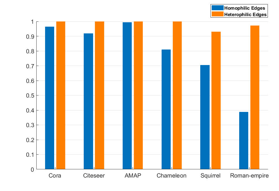
To overcome aforementioned drawbacks, we first investigate the commonality of neighbors in homophilic and heterophilic graph through empirical experiments. Our intuition comes from Balance theory [22, 23], which states: “My enemy’s enemy is my friend, my friend’s friend is also my friend.” Thus, for heterophilic graph, if two nodes have many common “enemies”, then these two nodes are highly possible to be classified into one cluster; for homophilic graph, two nodes that share many common “friends” are likely from the same cluster. We conduct some empirical experiments to verify this. Define an edge $E_{ij}$ that connects two nodes $v_i$ and $v_j$, and their neighbors are ${𝒩}_i$ and ${𝒩}_j$, respectively. We compute the proportion of common neighbors as: $\frac{{𝒩}_i\cap {𝒩}_j}{{𝒩}_i\cup {𝒩}_j}$. If $\frac{{𝒩}_i\cap {𝒩}_j}{{𝒩}_i\cup {𝒩}_j}\ge 0.5$, we classify $E_{ij}$ as homophilic edge. Otherwise, we treat $E_{ij}$ as a heterophilic edge since the connected nodes do not have enough common “friends” or “enemies”. We compute the proportions of edges that can be correctly classified in six real homophilic and heterophilic datasets. From Fig. 1, we can see that: 1) most edges can be correctly distinguished by neighbor information; 2) heterophilic edges can be identified with high precision. This interesting finding inspires us to fully exploit the neighbor information in a real graph process.

On the basis of the commonality, we first propose a simple method to build two graphs that are highly homophilic and heterophilic. Then a novel filter is designed taking into account their different neighborhood sizes, which is theoretically proven to be favorable for clustering. Also, a squeeze-and-excitation block is also employed to enhance essential features. Our main contributions are summarized as follows.

• We investigate the commonality of the neighbors of homophilic and heterophilic graphs. Based on it, we develop two unsupervised strategies for graph restructuring to capture homophilic and heterophilic information from any kinds of graphs.

• We propose a novel filter for real-world graph filtering and provide theoretical analysis to show its advantage.

• We make the first attempt to apply squeeze-and-excitation idea in graph clustering to boost essential features after aggregation.

II Related work

II-A Graph Clustering

Attributed graph clustering methods can be roughly divided into two categories. The first kind is GNNs-based methods. They learn the representations by adopting a message passing mechanism based on the topology structure [24]. DAEGC [25] is a goal-directed framework that combines an attention-based graph autoencoder with deep learning of latent representation. MSGA [26] introduces a multiscale self-expression module to obtain more discriminative coefficient representation from each encoder layer and a self-supervised module to supervise the learning process. SSGC [27] uses a modified Markov diffusion kernel to capture global and local contexts of each node, allowing aggregation in large neighborhoods while limiting severe oversmoothing. Contrastive learning idea is also widely used in graph clustering. CCGC [13] addresses the issue of semantic drift by using siamese encoders with unshared parameters and leveraging high-confidence cluster information to carefully select positive samples. SCGC [14] utilizes parameter unshared siamese encoders along with direct perturbation of node embeddings using Gaussian noise. The second kind is the shallow method without using neural networks. [28] and [29] acquire smooth embeddings through the utilization of low-pass filters. FGC [16] and MCGC [15] adopt the low-pass filter and learn the nearest neighbor information, respectively, for the new graph. Nevertheless, these methods focus only on homophilic graphs and ignore heterophily, which is limited, since real-world graphs always contain heterophilic edges.

II-B Learning on Heterophilic Graphs

Heterophilic graphs pose significant challenges for many GNN-based methods, leading to performance degradation. The heterophilic problem has been extensively studied in node classification tasks. Some methods have been proposed to expand the receptive field to find homophilic neighbors. MixHop [30] overcomes heterophily by iteratively blending feature representations of neighbors situated at different distances. GloGNN [21] constructs a graph that includes high-order neighbors to discern homophilic neighbors in the graph structure. Besides, many methods are proposed to revise the message-passing architecture for heterophilic graphs. ACM-GCN [31] adaptively employs aggregation, diversification, and identity channels in each layer to counter harmful heterophily and improve the performance of GNN. LINKX [32] segregates graph and feature representations.

Although these approaches mitigate the heterophilic problem to some extent, they heavily depend on prior knowledge, such as labels, which are not accessible in unsupervised tasks. To our knowledge, SELENE [33], CGC [34], and DGCN [35] are the only graph clustering methods that consider heterophily. SELENE [33] uses a dual-channel feature embedding pipeline to discriminate r-ego networks using node attributes and structural information separately. DGCN and CGC use an adaptive filter to capture meaningful low- and high-frequency information. However, these methods are based on traditional low-pass filers and ignore global structure information. The most related work to ours is DGCN, which also constructs a homophilic and a heterophilic graph for clustering. However, it has the following drawbacks with respect to our method: 1) It needs $O(N^4)$ computational complexity to build graphs, which makes it impossible to apply on even middle size graphs. 2) Its homophilic graph is solely based on features without taking into account the property of the original structure. 3) Its filter fails to incorporate global structure information.

III Methodology

Notations. We define an undirected graph $𝒢=(𝒱,E,X)$, where $𝒱=\{v_1,v_2,\mathrm{\dots },v_N\}$ represents the node set and $E$ denotes the edge set with $|E|$ edges. $X\in {ℝ}^{N\times d}$ is the feature matrix and $d$ is the number of channels. The matrix $A\in {ℝ}^{N\times N}$ signifies the adjacency matrix, where $A_{ij}=1$ if $(v_i,v_j)\in E$; otherwise, $A_{ij}=0$. Additionally, the matrix $D$ corresponds to the degree matrix with $D_{ii}={\sum }_j{A}_{ij}$. The normalized $A$ is $\tilde{A}=D^{-\frac{1}{2}}(A+I)D^{-\frac{1}{2}}$. The normalized Laplacian graph is $L=I-\tilde{A}=U\mathrm{\Lambda }{U}^{\top }$ and its eigenvalue matrix is $\mathrm{\Lambda }=diag({\lambda }_1,{\lambda }_1,\mathrm{\dots },{\lambda }_N)$, where $0\le {\lambda }_1\le {\lambda }_2\le \mathrm{\cdots }\le {\lambda }_N\le 2$. $U=\{u_1,\mathrm{\dots },u_N\}$ indicates corresponding orthonormal eigenvectors.

III-A Graph Restructuring

Graph clustering faces two critical challenges: real-world graphs are comprised of a mixture of both homophilic and heterophilic edges; graph homophily is unknown beforehand in clustering. Directly using the original graph for filtering would be detrimental to downstream clustering. Therefore, it is pressing to develop a principled way to cluster graphs with different levels of homophily. In this paper, we follow a graph restructuring approach that extracts homophily and heterophily information separately.

III-A1 Homophilic Graph Construction

On the basis of our previous finding of commonality, we use neighborhood information to distinguish homophilic and heterophilic edges. Specifically, we use Cosine similarity to compute the distance between nodes in attribute and topology space:

$K_{ij}={\displaystyle \frac{X_{i,:}^{\top }\cdot X_{j,:}}{\Vert X_{i,:}\Vert \Vert X_{j,:}\Vert }}$ (1)

$B_{ij}={\displaystyle \frac{A_{i,:}^{\top }\cdot A_{j,:}}{\Vert A_{i,:}\Vert \cdot \Vert A_{j,:}\Vert }}$

$i,j\in [1,2,\mathrm{\cdots }N],$

where $X_{i,:}$ is the $i$-th row of $X$. Then homophilic graph $M$ is constructed as follows:

$M=K\odot B,$ (2)

where $\odot$ is the Hadamard product, which is used to screen common neighbors in both the attribute and the topology space. $ϵ$ is set to 0.001 or 0.05 to eliminate some noise.

III-A2 Heterophilic Graph Construction

We use the complementary graph idea to build heterophilic graph $G$ as follows:

$\overline{K}=1.-K$ (3)

$\overline{M}=1.-M$

$G=\overline{K}\odot \overline{M},$

where 1. is the matrix with all 1s. $G$ characterizes similar nodes that are far away in the topology space. We use $M$ instead of $A$ since neighbors in $M$ are more likely to be homophilic neighbors. $G$ could be dense, so we retain only five edges for each node, corresponding to the top five distant nodes.

Figure 2: The overall architecture of our proposed method.

III-B Clustering Framework

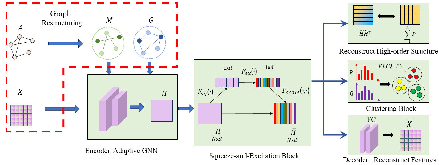
Our overall framework for the graph clustering task is shown in Fig. 2. It first encodes the node features with a novel filter, using our constructed graphs $G$ and $M$. Then, we improve the learned representation with a squeeze-and-excitation block, which consists of two steps, i.e., squeeze and excitation operation. The decoder is applied to reconstruct the original features $X$. The clustering block is applied to enhance clustering performance.

III-B1 Graph Filtering

Previous research finds that low-frequency filters have a positive correlation with homophily, while high-frequency filters have a negative correlation [36]. Treating the graphs $M$ and $G$ differently, we perform homophilic aggregation and heterophilic aggregation respectively.

Homophilic aggregation: Traditional GNNs [24] only aggregate local information, which loses information. Thus, we consider the global filter: $F=\exp (g(L))$, where $g(L)$ is a linear filter that can capture low- or high-frequency information. To capture low-frequency information, we adopt GCN’s filter kernel, i.e., for graph $M$, we have $g_1({\tilde{L}}_M)=I-{\tilde{L}}_M$, where ${\tilde{L}}_M=U_{1}diag\{{\lambda }_1^{(1)},{\lambda }_2^{(1)},\mathrm{\dots },{\lambda }_N^{(1)}\}{U}_1^{\top }$ is the restructured graph $M$’s normalized Laplacian matrix. Then the global GNN becomes:

$F=\exp (M).$ (4)

The reason for using this global low-pass filter can be explained by the Taylor expansion as follows:

$$\exp (M)=\sum _{n\ge 0}\frac{M^n}{n!}.$$ (5)

It can describe global information since $\exp {(M)}_{ij}\ne 0$ if a path with distinct hops connects nodes $v_i$ and $v_j$. A high value of $M_{ij}$ means that in the $n$ hops, there is a great similarity between $v_i$ and $v_j$. The factorial division guarantees that the whole infinite sum exists by preserving mathematical stability using factors that rapidly approach zero. As a result, the important weight will decrease substantially as the hop increases. This is consistent with the characteristic of the homophilic graph since the possibility of homophilic nodes decreases as the hop increases [21].

Heterophilic aggregation: To capture high-frequency information, we use traditional local GNN [37]:

$$F=U_2\mathrm{diag}\left({\left\{\frac{{\lambda }_i}{{\lambda }_N}\right\}}_{i=1}^N\right)U_2^{\top }=\frac{1}{{\lambda }_N}{\tilde{L}}_G=\frac{2}{3}{\tilde{L}}_G,$$ (6)

where ${\tilde{L}}_G=U_{2}diag\{{\lambda }_1^{(2)},{\lambda }_2^{(2)},\mathrm{\dots },{\lambda }_N^{(2)}\}{U}_2^{\top }$ is restructured graph $G$’s normalized Laplacian matrix. $\frac{1}{{\lambda }_N}$ is always set to $\frac{2}{3}$ according to previous work [37].

Adaptive GNN: Homophilic and heterophilic neighboring nodes appear in both homophilic and heterophilic graphs. As a result, we combine the above low- and high-pass filters and propose the aggregation of the $l$-th layer as follows:

$H^{(l)}$ $=(1-\mu )U_1\mathrm{diag}\left({\left\{e^{1-{\lambda }_i^{(1)}}\right\}}_{i=1}^N\right)U_1^{\top }{H}^{(l-1)}{W}^{(l-1)}$ (7)

$+\mu \left({\displaystyle \frac{2}{3}}{\tilde{L}}_G\right)W^{(l-1)}.$

The global filter is Min-Max normalized to have the same range as the local filter, and $\mu$ is a trade-off parameter that balances low- and high-frequency information. $H^{(0)}$ is the original feature $X$. With this aggregation, our model can adaptively aggregate low- and high-frequency information in each layer. The reason why we use global aggregation on the homophilic graph while using local aggregation on the heterophilic graph is analyzed in the theorem III.1.

III-B2 Squeeze-and-excitation Block

After encoding, we fed the obtained node representation $H$ into squeeze-and-excitation (SE) block, which is an attention mechanism based on attribute dimensions. Significant node features will be improved. It consists of two major steps: Squeeze and Excitation.

Squeeze: To consider global features in latent space, the squeeze operation compresses the node representation $N\times d$ into $1\times d$. Specifically, squeeze operation is global pooling as follows:

$$s=F_{sq}\left(H\right)=\frac{1}{N}\sum _{i=1}^N{H}_{i,:},$$ (8)

where $s\in {ℝ}^{1\times d}$, which is considered to be a channel-wise statistic that squeezes global feature information.

Excitation: Excitation follows the squeeze operation and aims to capture all dependencies among channels. Excitation is a simple gating mechanism, which enables flexibility in learning nonlinear interactions between channels. It uses the sigmoid function $\sigma$ to excite the squeezed feature map. First, the dimension decreases through the fully connected layer. Then we use a ReLU function $\delta \left(\right)$ and a fully connected layer with increasing dimensionality to return dimensions, that is, $W_2\delta \left(W_{1}s\right)$. Finally, the sigmoid function is applied to it. The operation is summarized as follows:

$\tilde{s}$ $=F_{ex}(s,W)=\sigma \left(W_2\delta \left(W_{1}s\right)\right).$ (9)

Reweight: The result of the excitation operation is considered to be the importance of each attribute due to the selection of the attribute dimension. Next, we finish recalibrating the representations by multiplying each attribute dimension by the initial representations $H$. The specific reweight operation is defined as follows:

$$\tilde{H}=F_{scale}(H,\tilde{s})=\tilde{s}H,$$ (10)

where $\tilde{H}$ is the output of SE block.

III-B3 Clustering Module

Existing works often reconstruct the original topology structure [25], which makes neighboring nodes have similar representations. However, this is based on the homophily assumption. Reconstructing a heterophilic graph would make highly dissimilar nodes close. As pointed out by [21], homophilic nodes exist in multihop neighbors. Thus, we propose reconstructing the high-order topology structure as follows.

$${ℒ}_{HS}=\frac{1}{N^2}{\Vert \tilde{H}{\tilde{H}}^{\top }-\sum _{i=1}^k{\tilde{A}}^i\Vert }_F^2,$$ (11)

where $k$ indicates reconstructing $k$-order structure.

The decoder is applied to reconstruct the original features $X$. Some ”easy” nodes show few feature variations during reconstruction, suggesting their trivial contribution to model training. We adopt the fully connected (FC) layer as the decoder with output $\overline{X}$ and Scaled Cosine Error (SCE) [38] as the objective function:

$${ℒ}_{\mathrm{RE}}=\sum _{i=1}^N{\left(1-\frac{X_{i,:}^{\top }{\overline{X}}_{i,:}}{\Vert X_{i,:}\Vert \cdot \Vert {\overline{X}}_{i,:}\Vert }\right)}^2.$$ (12)

Finally, we utilize a clustering block for cluster enhancement. The soft assignment distribution $P$ is calculated as:

$$p_{ij}=\frac{{\left(1+{\Vert {\tilde{H}}_{i,:}-c_j\Vert }^2/\beta \right)}^{-\frac{\beta +1}{2}}}{{\sum }_{j^{\prime }}{\left(1+{\Vert {\tilde{H}}_{i,:}-c_{j^{\prime }}\Vert }^2/\beta \right)}^{-\frac{\beta +1}{2}}},$$ (13)

where cluster centers $c$ are initialized using K-means on the representations and $\beta$ represents the degree of freedom in the Student’s $t$-distribution. The target distribution $Q$ is computed as:

$$q_{ij}=\frac{p_{ij}^2/{\sum }_i{p}_{ij}}{{\sum }_{j^{\prime }}\left(p_{i{j}^{\prime }}^2/{\sum }_i{p}_{i{j}^{\prime }}\right)}.$$ (14)

We improve the cohesiveness of the cluster by bringing the node representation closer to the cluster centers by minimizing the KL divergence between the distributions $P$ and $Q$, which is calculated as:

$${ℒ}_{CLU}=KL(Q\parallel P)=\sum _i\sum _j{q}_{ij}\log \frac{q_{ij}}{p_{ij}}$$ (15)

Eventually, the objective function of our proposed Provable Filter for Graph Clustering (PFGC) method is formulated as:

$$ℒ={ℒ}_{RE}+{\gamma }_1{ℒ}_{HS}+{\gamma }_2{ℒ}_{CLU},$$ (16)

where ${\gamma }_1$ and ${\gamma }_2$ are trade-off parameters to balance three terms. We minimize the objective function above to train the model, obtaining the clustering label for node $i$ as:

$$z_i=\underset{𝑗}{\mathrm{argmax}{p}_{ij}}.$$ (17)

III-C Computational Complexity

PFGC’s complexity mainly comes from the graph restructuring and adaptive GNN. The complexity of cosine similarity is $O(N^2)$. A sampling strategy can be applied to make it linear to the number of nodes. Adaptive GNN necessitates the eigendecomposition of the graph Laplacian. Empirically, there are two approaches to enhance its speed. Firstly, the graph’s eigendecomposition results can be stored and accessed after a one-time computation, thus, we only require a single eigendecomposition. Second, although the filtering process occurs in the spectral domain, empirically, the polynomial approximation can be used to approximate this process. Consequently, the computational complexity of adaptive GNN is comparable to that of standard linear GCN [24] and graph diffusion models [39].

III-D Theoretical Analysis of Filter Behaviors

For graph clustering, the theory connection between filter and clustering performance remains underexplored. To fill this gap, we theoretically analyze how to design the filters to better suit the practical graphs with different homophily levels. The characteristics of homophilic and heterophilic graphs require a different neighborhood size for filtering. We consider the local filter with a small receptive field and the global filter with a large receptive field. Assume that the graph is balanced and undirected, having $N$ nodes and $C$ clusters with $N/C$ nodes for each category. Its Laplacian matrix is $L$ with a maximum eigenvalue ${\lambda }_N$. Consider global filters: $h_1(L)=\exp (I-L)$, $h_3(L)=\exp (L)$ and local filters that are widely applied in other methods: $h_2(L)=I-\frac{1}{{\lambda }_N}L$, $h_4(L)=\frac{1}{{\lambda }_N}L$. Global filters are Min-Max normalized to have the same range as local filters, which is consistent with our proposed methods. $r$ is homophily ratio. Then we have the following theorem:

Theorem III.1.

Assume that low-pass and high-pass filters are applied on the graphs with $r\mathrm{>}\frac{\mathrm{1}}{C}$ and , respectively. Then the clusters would be more discriminative with $h_{\mathrm{1}}\mathit{}\mathrm{(}L\mathrm{)}$ compared to $h_{\mathrm{2}}\mathit{}\mathrm{(}L\mathrm{)}$, while $h_{\mathrm{4}}\mathit{}\mathrm{(}L\mathrm{)}$ improves the discriminativeness of the clusters more than $h_{\mathrm{3}}\mathit{}\mathrm{(}L\mathrm{)}$.

Proof.

$x$ is the original graph signal. ${\overline{x}}^{(i)}$ is the filtered representation by $h_i(L)$ (i=1,2,3,4). Let $S_{in}^{(i)}$ and $S_{out}^{(i)}$ be the total intra-cluster and inter-cluster distance; ${\overline{S}}_{in}^{(i)}$ and ${\overline{S}}_{out}^{(i)}$ be the average intra-cluster and inter-cluster distance of $x^{(i)}$. $𝔼\left[S^{(i)}\right]=𝔼\left[S_{out}^{(i)}-S_{in}^{(i)}\right]$ and $𝔼\left[{\overline{S}}^{(i)}\right]=𝔼\left[{\overline{S}}_{out}^{(i)}-{\overline{S}}_{in}^{(i)}\right]$. We can represent signal $x$ as the linear combination of the eigenvectors:

$$x=\sum _{t=1}^N{a}_t{u}_t,$$ (18)

where $a_t=u_t^{\top }x$ is the coefficient. Then the filtered signal can be calculated as:

$\overline{x}$ $=h(L)x=Uh(\mathrm{\Lambda })U^{\top }x$ (19)

$=\left({\displaystyle \sum _{t=1}^N}h\left({\lambda }_t\right)u_t{u}_t^{\top }\right)\left({\displaystyle \sum _{t=1}^N}{a}_t{u}_t\right)={\displaystyle \sum _{t=1}^N}h\left({\lambda }_t\right)a_t{u}_t.$

Filtered signals with $h_1(L)$, $h_2(L)$, $h_3(L)$, $h_4(L)$ are ${\overline{x}}^{(1)}$, ${\overline{x}}^{(2)}$, ${\overline{x}}^{(3)}$, ${\overline{x}}^{(4)}$, respectively. The smoothness of the neighboring nodes can be calculated as:

$$\begin{array}{c}\sum _{i,j\in E}{\left(x_i-x_j\right)}^2=x^{\top }Lx\\ \sum _{i,j\in E}{\left({\overline{x}}_i-{\overline{x}}_j\right)}^2=x^{\top }h(L)x\end{array}$$ (20)

The eigenvector’s smoothness score and its corresponding eigenvalue are equivalent:

$${\lambda }_t=u_t^{\top }L{u}_t=\sum _{i,j\in E}{\left(u_{t,i}-u_{t,j}\right)}^2$$ (21)

We have:

${\displaystyle \sum _{(i,j)\in E}}{\left({\overline{x}}_i-{\overline{x}}_j\right)}^2$ (22)

$=\left({\displaystyle \sum _{t=1}^N}h\left({\lambda }_t\right)a_t{u}_t^{\top }\right)\left({\displaystyle \sum _{t=1}^N}{\lambda }_t{u}_t{u}_t^{\top }\right)\left({\displaystyle \sum _{t=1}^N}h\left({\lambda }_t\right)a_t{u}_t\right)$

$={\displaystyle \sum _{t=1}^N}{a}_t^2{\lambda }_t{h}^2\left({\lambda }_t\right)$

Since $x$ is an arbitrary unit graph signal, all $a_t$’s are independently identically distributed (i.i.d.). For i.i.d. random variables $a_i$ and $a_j$ ($j>i$), we have:

$𝔼\left(a_i^2\right)=𝔼\left(a_j^2\right)$ (23)

$\Rightarrow {\lambda }_i𝔼\left[a_i^2\right]=𝔼\left[{\lambda }_i{a}_i^2\right]⩽𝔼\left[{\lambda }_j{a}_j^2\right]={\lambda }_j𝔼\left[a_j^2\right]$

Then, we can calculate the total distance between neighboring nodes after filtering. $\mathrm{\Delta }d$ is the distance between the global and local filters. Specifically, the distance between $x^{(1)}$ and $x^{(2)}$ can be calculated as:

$𝔼[\mathrm{\Delta }d]$ $=𝔼\left[{\displaystyle \sum _{i,j\in E}}{\left({\overline{x}}_i^{(1)}-{\overline{x}}_j^{(1)}\right)}^2\right]-𝔼\left[{\displaystyle \sum _{i,j\in E}}{\left({\overline{x}}_i^{(2)}-{\overline{x}}_j^{(2)}\right)}^2\right]$ (24)

$=𝔼\left[{\displaystyle \sum _{t=1}^N}{a}_t^2{\lambda }_t{h}_1^2\left({\lambda }_t\right)\right]-𝔼\left[{\displaystyle \sum _{t=1}^N}{a}_t^2{\lambda }_t{h}_2^2\left({\lambda }_t\right)\right]$

$={\displaystyle \sum _{t=1}^N}\left\{\left[h_1^2\left({\lambda }_t\right)-h_2^2\left({\lambda }_t\right)\right]{\lambda }_t𝔼\left[a_t^2\right]\right\}$

$={\displaystyle \sum _{t=1}^N}\left\{\left[{\left({\displaystyle \frac{e^{1-{\lambda }_t}-e^{1-{\lambda }_N}}{e^{1-{\lambda }_1}-e^{1-{\lambda }_N}}}\right)}^2-{\left(1-{\displaystyle \frac{{\lambda }_t}{{\lambda }_N}}\right)}^2\right]{\lambda }_t𝔼\left(a_t^2\right)\right\}$

Note that our global filter is Min-Max normalized to ensure it has the same range as local filter. Define a general function $g_0(\lambda )$ regarding $\lambda$:

$g_0(\lambda )={\left({\displaystyle \frac{e^{1-\lambda }-e^{1-{\lambda }_N}}{e^{1-{\lambda }_1}-e^{1-{\lambda }_N}}}\right)}^2-{\left(1-{\displaystyle \frac{\lambda }{{\lambda }_N}}\right)}^2$ (25)

$=\left({\displaystyle \frac{e^{1-\lambda }-e^{1-{\lambda }_N}}{e^{1-{\lambda }_1}-e^{1-{\lambda }_N}}}+1-{\displaystyle \frac{{\lambda }_t}{{\lambda }_N}}\right)\left({\displaystyle \frac{e^{1-\lambda }-e^{1-{\lambda }_N}}{e^{1-{\lambda }_1}-e^{1-{\lambda }_N}}}-1+{\displaystyle \frac{\lambda }{{\lambda }_N}}\right)$

$\lambda \in \{{\lambda }_1,{\lambda }_2,\mathrm{\cdots },{\lambda }_N\}$

Define $g_1(\lambda )=\frac{e^{1-\lambda }-e^{1-{\lambda }_N}}{e^{1-{\lambda }_1}-e^{1-{\lambda }_N}}+1-\frac{1}{{\lambda }_N}\lambda$ and $g_2(\lambda )=\frac{e^{1-\lambda }-e^{1-{\lambda }_N}}{e^{1-{\lambda }_1}-e^{1-{\lambda }_N}}-1+\frac{1}{{\lambda }_N}\lambda$. Obviously, $g_1(\lambda )$ is monotonically decreasing with respect to $\lambda$, so $g_1(\lambda )\ge g_1\left({\lambda }_N\right)=0$. Therefore, we only need to focus on $g_2(\lambda )$ to judge whether $g_0(\lambda )$ is positive or negative. Let $g_2^{\prime }(\lambda )$=0, we have:

$\overline{\lambda }=1+\ln \left(e^{1-{\lambda }_1}-e^{1-{\lambda }_N}\right)+\ln {\lambda }_N>0$ (26)

Thus $g_2(\lambda )$ is monotonically decreasing on $(0,\overline{\lambda })$ and monotonically increasing on $(\overline{\lambda },+\mathrm{\infty })$. Considering $g_2({\lambda }_N)=0$, $g_0(\lambda )=0$ only has one root ${\lambda }_0$ in $({\lambda }_1,{\lambda }_N)$. Thus $g_0(\lambda )$$\ge 0$ when ${\lambda }_t\in [{\lambda }_1,{\lambda }_m]$ and $g_0(\lambda )$$\le 0$ when ${\lambda }_t\in [{\lambda }_{m+1},{\lambda }_N]$, where ${\lambda }_m$ is the closest one to ${\lambda }_0$ in ${\lambda }_t\le {\lambda }_0$. Note that both filters are applied on the reconstructed homophilic graph, which indicates ${\lambda }_1$ is very close to 0. Thus, ${\lambda }_0$ and $g_0{(\lambda )}_{max}=(2-\frac{{\lambda }_1}{{\lambda }_N})\frac{{\lambda }_1}{{\lambda }_N}$ are very close to 0. Therefore, we assume that ${\Vert {[g_0\left({\lambda }_1\right),\mathrm{\cdots },g_0\left({\lambda }_m\right)]}^{\top }\Vert }_2^2\le {\Vert {[g_0\left({\lambda }_{m+1}\right),\mathrm{\dots },g_0\left({\lambda }_N\right)]}^{\top }\Vert }_2^2$. Then we have the following:

$0⩽{\displaystyle \sum _{t=1}^m}\left[h_1^2\left({\lambda }_t\right)-h_2^2\left({\lambda }_t\right)\right]⩽{\displaystyle \sum _{m+1}^N}\left[h_2^2\left({\lambda }_t\right)-h_1^2\left({\lambda }_t\right)\right]$ (27)

$\Rightarrow$ $0⩽{\displaystyle \sum _{t=1}^m}\left[h_1^2\left({\lambda }_t\right)-h_2^2\left({\lambda }_t\right)\right]{\lambda }_t$

$\le {\lambda }_{m+1}{\displaystyle \sum _{m+1}^N}\left[h_2^2\left({\lambda }_t\right)-h_1^2\left({\lambda }_t\right)\right]$

We can derive the following result from it:

(28)

Similarly, we can prove the following conclusion with high-pass filters:

$𝔼\left[\mathrm{\Delta }{d}^{\prime }\right]$ (29)

$=𝔼\left[{\displaystyle \sum _{i,j\in E}}{\left({\overline{x_i}}^{(3)}-{\overline{x_j}}^{(3)}\right)}^2\right]-𝔼\left[{\displaystyle \sum _{i,j\in E}}{\left({\overline{x_i}}^{(4)}-{\overline{x_j}}^{(4)}\right)}^2\right]$

Define $z_i$ as the label of node $i$. We can compute the total intra-cluster and inter-cluster distance as follows:

$𝔼\left[S_{in}^{(1)}-S_{in}^{(2)}\right]=𝔼\left[r\mathrm{\Delta }d\right]$ (30)

$=𝔼\left[{\displaystyle \sum _{\begin{array}{c}i,j\in E\\ z_i=z_j\end{array}}}\left[{\left({\overline{x}}_i^{(1)}-{\overline{x}}_j^{(1)}\right)}^2-{\left({\overline{x}}_i^{(2)}-{\overline{x}}_j^{(2)}\right)}^2\right]\right]$

$𝔼\left[S_{out}^{(1)}-S_{out}^{(2)}\right]=𝔼\left[(1-r)\mathrm{\Delta }d\right]$

$=𝔼\left[{\displaystyle \sum _{\begin{array}{c}i,j\in E\\ z_i\ne z_j\end{array}}}\left[{\left({\overline{x}}_i^{(1)}-{\overline{x}}_j^{(1)}\right)}^2-\left({\overline{x}}_i^{(2)}-{\overline{x}}_j^{(2)}\right)\right]\right]$

Finally, the average distance between inter-cluster and intra-cluster nodes can be calculated as:

$𝔼\left[{\overline{S}}^{(1)}-{\overline{S}}^{(2)}\right]$ (31)

$=𝔼\left[({\overline{S}}_{out}^{(1)}-{\overline{S}}_{out}^{(2)})-({\overline{S}}_{in}^{(1)}-{\overline{S}}_{in}^{(2)})\right]$

$={\displaystyle \frac{2C(1-r)𝔼\left[\mathrm{\Delta }d\right]}{N^2(C-1)}}-{\displaystyle \frac{2Cr𝔼\left[\mathrm{\Delta }d\right]}{N^2}}$

$={\displaystyle \frac{2C}{(C-1)N^2}}\left[𝔼\left[\mathrm{\Delta }d\right](1-Cr)\right]$

Similarly, after high-pass filtering, we have:

$𝔼\left[{\overline{S}}^{(3)}-{\overline{S}}^{(4)}\right]$ (32)

$={\displaystyle \frac{2C}{(C-1)N^2}}\left[𝔼\left[\mathrm{\Delta }{d}^{\prime }\right](1-Cr)\right]$

Obviously, $\frac{2C}{(C-1)N^2}>0$. We reach the following conclusions.

(1) If $r>\frac{1}{C}$, then $𝔼\left[{\overline{S}}^{(1)}-{\overline{S}}^{(2)}\right]>0$, that is, $𝔼\left[{\overline{S}}^{(1)}\right]>𝔼\left[{\overline{S}}^{(2)}\right]$

(2) If , then , that is, ∎

Therefore, the clusters are more discriminative after applying a global filter to a homophilic graph, whereas they are more discriminative with a local filter on a heterophilic graph. Connected nodes of a homophilic graph are more possible from the same cluster, while the opposite is true for a heterophilic graph. Thus, a combination of global and local filters can make the clusters more distinguishable by reducing intra-cluster distance and increasing inter-cluster distance. This explains why the proposed adaptive GNN is more suitable for the real-world graph process.

IV Experiments

IV-A Datasets

For fairness, we select benchmark datasets commonly used for graph clustering tasks. For the homophilic graph, we opt for five datasets: Cora, CiteSeer, Pubmed [40], Amazon Photo (AMAP) [41], USA Air-Traffic (UAT) [42]. For the heterophilic graph, six datasets are chosen, Chameleon and Squirrel are page-page networks focused on specific topics sourced from Wikipedia [43]; Carnegie Mellon University collected webgraphs from multiple computer science departments at various universities, including Cornell, Wisconsin, and Washington. Roman-empire is derived from the Roman Empire article on English Wikipedia, chosen as one of the longest articles available on the platform [44]. The calculation of the homophily ratio follows [45], where a large value indicates high homophily. The statistics of these datasets are summarized in Table I.

TABLE I: Statistics information of datasets.

Graph datasets		Nodes	Dims.	Edges	Clusters	Homophily Ratio
Heterophilic Graphs	Cornell	183	1703	298	5	0.1220
	Wisconsin	251	1703	515	5	0.1703
	Washington	230	1703	786	5	0.1434
	Chameleon	2277	2325	31371	5	0.2299
	Squirrel	5201	2089	217073	5	0.2234
	Roman-empire	22662	300	32927	18	0.0469
Homophilic Graphs	Cora	2708	1433	5429	7	0.8137
	Citeseer	3327	3703	4732	6	0.7392
	Pubmed	19717	500	44327	3	0.8024
	UAT	1190	239	13599	4	0.6978
	AMAP	7650	745	119081	8	0.8272

IV-B Comparison Methods

To showcase the superiority of our PFGC, we compare it against 18 baselines for performance evaluation. These 18 baselines cover five distinct categories of methods: 1) traditional GNN-based methods, such as DAEGC [25], MSGA [26], SSGC [46], GMM [47], RWR [48], ARVGA [11]; 2) contrastive learning-based methods, such as MVGRL [49], SDCN [50], DFCN [51], DCRN [52], SCGC [14], and CCGC [13], leveraging MLPs and GNNs together to learn an aligned representation from augmented perspectives; 3) the advanced clustering approach AGE [53], which achieves clustering-friendly embbedings through Laplacian smoothing filters and adaptive encoders; 4) shallow methods that utilize the filter to smooth raw features and reduce noise, including MCGC [15], FGC [16] and CGC [34]; (5) recent methods that unify homophily and heterophily, including SELENE [33] and DGCN [35].

TABLE II: Results on heterophilic graphs. The best results are bolded with red and the second-best performance is also bolded. ”OOM” indicates out of memory.

Methods	Cornell		Wisconsin		Washington		Chameleon		Squirrel		Roman-empire
	ACC	NMI	ACC	NMI	ACC	NMI	ACC	NMI	ACC	NMI	ACC	NMI
DAEGC	42.56	12.37	39.62	12.02	46.96	17.03	32.06	6.45	25.55	2.36	21.23	12.67
MSGA	50.77	14.05	54.72	16.28	49.38	6.38	27.98	6.21	27.42	4.31	19.31	12.25
FGC	44.10	8.6	50.19	12.92	57.39	21.38	36.50	11.25	25.11	1.32	14.46	4.86
GMM	58.86	-	52.08	8.89	60.86	20.56	-	-	-	-	-	-
RWR	58.29	-	53.96	16.02	63.91	23.13	-	-	-	-	-	-
ARVGA	56.23	-	56.23	13.73	60.87	16.19	-	-	-	-	-	-
DCRN	51.32	9.05	57.74	19.86	55.65	14.15	34.52	9.11	30.69	6.84	32.57	29.50
SELENE	57.96	17.32	71.69	39.51	-	-	38.97	20.63	-	-	-	-
CGC	44.62	14.11	55.85	23.03	63.20	25.94	36.43	11.59	27.23	2.98	30.16	27.25
DGCN	62.29	29.93	71.71	41.29	69.13	28.22	36.14	11.23	31.34	7.24	OOM	OOM
PFGC	66.12	33.04	74.10	47.53	70.43	37.99	41.28	21.62	33.05	7.58	33.98	38.80

IV-C Experimental Setting

To ensure fairness, all experimental settings in different data sets adhere to the DGCN [35], which performs a grid search to find the best results. Our network undergoes training with the Adam optimizer for 200 epochs until convergence. According to [21], more than half of the homophilic neighbors can be included in 5 hops. Thus, the hyper-parameter $k$ is fixed to 1 on Roman-empire and Pubmed to save computing time, and empirically set to 5 on other datasets. The optimizer’s learning rate is set between 1e-2 and 1e-3. ${\gamma }_1$ and ${\gamma }_2$ are chosen to balance the three types of loss in [1e-3, 1e-2, 1e-1, 1, 10]. We tune the trade-off parameter $\mu$ from 0.1 to 0.7. ACCuracy (ACC) and Normalized Mutual Information (NMI) are adopted as clustering metrics.

IV-D Results

The clustering results in heterophilic graphs are shown in Table II. It can be seen that PFGC has a dominant performance on all datasets. In particular, our method outperforms SELENE, CGC, and DGCN which consider heterophily. SELENE is a GNN-based method and both DGCN and CGC use adaptive filters. This verifies that our adaptive filter can better utilize graph information than them. In particular, these methods focus only on local information, while our method considers a global cluster structure. In addition to them, ACC of PFGC can surpass other methods by up to 9% on Cornell, 16% on Wisconsin, and 6% on Washington. This verifies that considering heterophily can make the model more powerful on real-world datasets. Moreover, traditional GNN-based approaches exhibit poor performance on heterophilic graphs, which is consistent with previous observations in the literature.

The clustering results in homophilic graphs are shown in Table III. It can be seen that PFGC shows competitive performance, achieving the best performance in most cases and ranking second in the remaining three cases. It is observed that state-of-the-art contrastive learning methods yield unstable performance. This instability is due to their performance, which is heavily based on the data augmentation strategy, which requires domain knowledge and lacks flexibility across different datasets. In the case of shallow methods, FGC and MCGC use only a low-pass filter. Their performance varies considerably between different datasets. CGC is the shallow method with an adaptive filter and shows better performance than FGC and MCGC. This verifies that a single filter is unsuitable for real graphs exhibiting various levels of homophily. PFGC and DGCN perform better than AGE in most cases, which shows that filtering only with a low-pass filter is not enough and high-frequency information is also important in homophilic cases. PFGC can surpass DGCN in all cases. This is partly because the new graphs in DGCN are constructed without taking into account the original structure property, which makes DGCN less effective in strong homophily graphs.

In summary, PFGC achieves stable and promising performance in both homophilic and heterophilic cases. This is primarily due to the ability of the graph to capture the homophilic and heterophilic information inherent in the graphs. Therefore, PFGC is suitable for clustering practical graphs, even when the homophily ratios are unknown.

TABLE III: Results on homophilic graphs.

Methods	Cora		Citeseer		Pubmed		UAT		AMAP
	ACC	NMI	ACC	NMI	ACC	NMI	ACC	NMI	ACC	NMI
DFCN	36.33	19.36	69.50	43.9	-	-	33.61	26.49	76.88	69.21
DCRN	48.93	-	70.86	45.86	-	-	-	-	79.94	73.70
SSGC	69.60	54.71	69.11	42.87	-	-	36.74	8.04	60.23	60.37
MVGRL	70.47	55.57	68.66	43.66	-	-	44.16	21.53	45.19	36.89
SDCN	60.24	50.04	65.96	38.71	65.78	29.47	52.25	21.61	53.44	44.85
AGE	73.50	57.58	70.39	44.92	-	-	52.37	23.64	75.98	-
MCGC	42.85	24.11	64.76	39.11	66.95	32.45	41.93	16.64	71.64	61.54
FGC	72.90	56.12	69.01	44.02	70.01	31.56	53.03	27.06	71.04	-
SCGC	73.88	56.10	71.02	45.25	67.73	28.65	56.58	28.07	77.48	67.67
CCGC	73.88	56.45	69.84	44.33	68.06	30.92	56.34	28.15	77.25	67.44
CGC	75.15	56.90	69.31	43.61	67.43	33.07	49.58	17.49	73.02	63.26
DGCN	72.19	56.04	71.27	44.13	OOM	OOM	52.27	23.54	76.07	66.13
PFGC	76.51	58.25	71.90	45.45	72.89	33.30	56.81	29.33	78.50	70.81

(a) Cora with restructured graph

(b) Cora with raw graph $A$

(c) Washington with restructured graph

(d) Washington with raw graph $A$

Figure 3: The effect of $k$ and $\mu$ on Cora and Washington with restructured graphs and raw graphs.

Figure 4: The effect of ${\gamma }_1$ and ${\gamma }_2$ on Cora (left) and Washington (right).

TABLE IV: Results of ablation study. The best performance is marked in bold.

Methods	PFGC w/o SE		PFGC-1		PFGC-2		PFGC-3		PFGC
	ACC	NMI	ACC	NMI	ACC	NMI	ACC	NMI	ACC	NMI
Cora	75.18	57.20	75.88	56.94	76.07	57.91	75.30	57.85	76.51	58.25
AMAP	75.88	67.90	75.38	67.54	78.38	70.25	76.26	67.82	78.50	70.81
Wisconsin	72.51	47.47	72.11	47.42	70.92	43.59	68.53	34.87	74.10	47.53
Washington	68.53	35.06	67.21	36.69	64.78	33.86	61.30	32.19	70.43	37.99

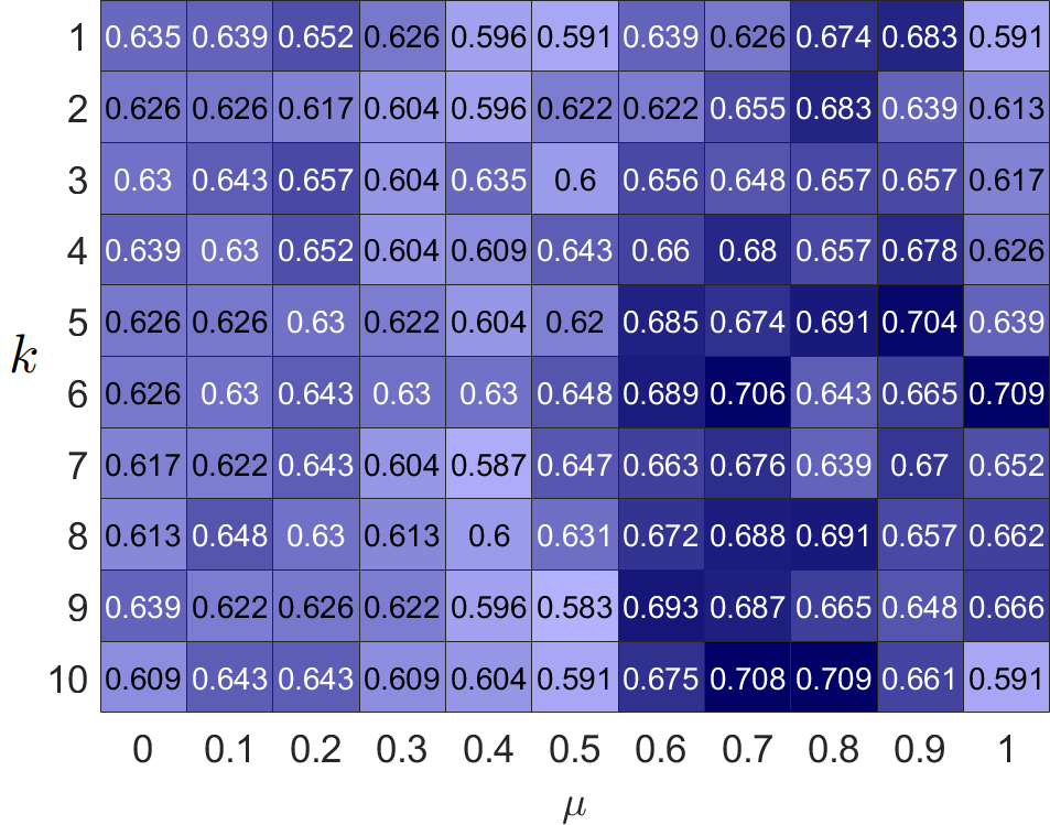
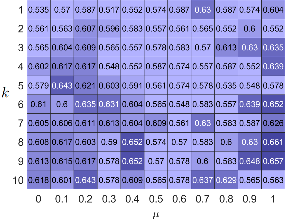
V Parameter analysis

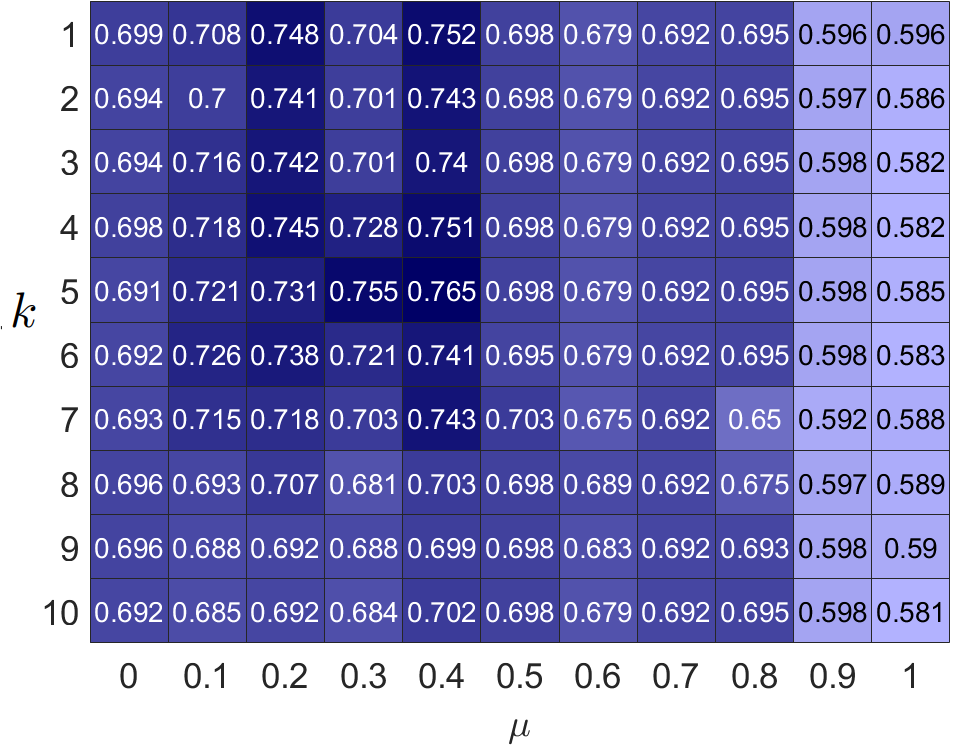
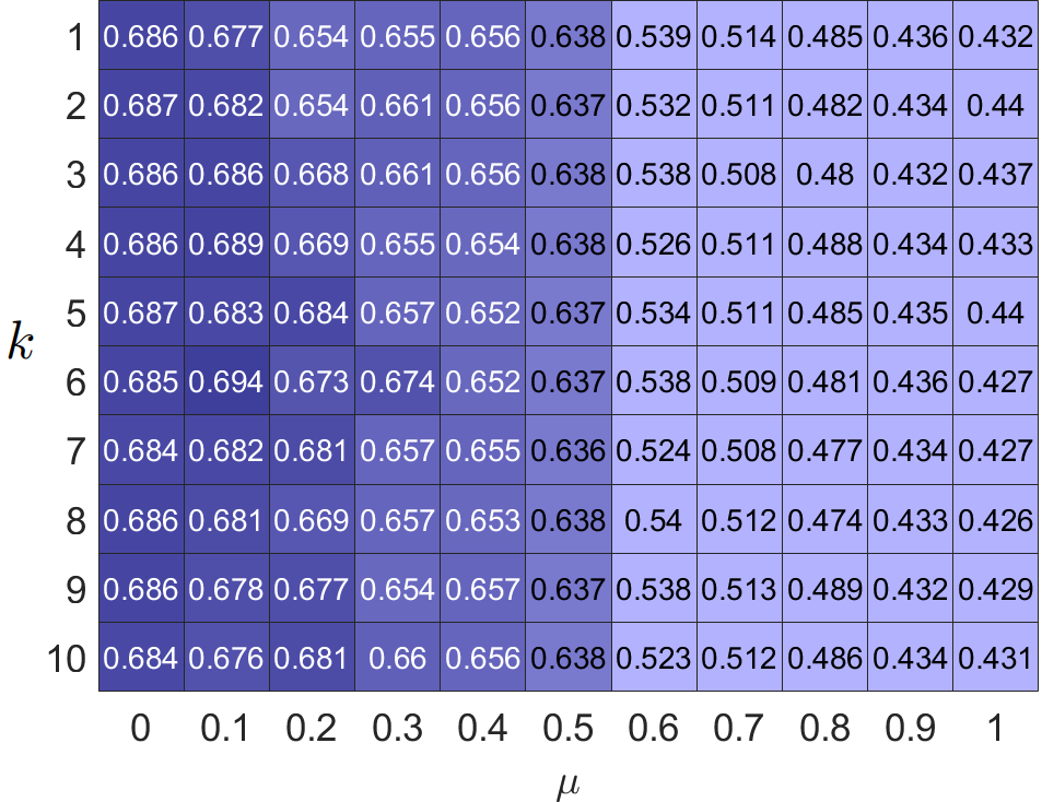
Our filter operates on newly restructured homophilic and heterophilic graphs, where neighboring nodes exhibit tendencies toward similarity and dissimilarity. Furthermore, our loss introduces a method to reconstruct structural information of order $k$. To demonstrate the effectiveness of restructured graphs and high-order structures, we evaluate the clustering accuracy of PFGC across hyper-parameters $\mu$ and $k$ in different graphs. The results are shown in Fig. 3. It can be seen that restructuring graphs significantly enhance model performance on both homophilic and heterophilic graphs. Furthermore, optimal performance occurs consistently when $\mu \ne 0$, indicating the importance of integrating high-frequency information. The homophilic graph achieves the best performance when $\mu$ is small, while the heterophilic graphs prefer large $\mu$, suggesting that the homophilic graphs tend to favor low-frequency components, while the heterophilic graphs exhibit sensitivity toward high-frequency components. We can also see that performance decreases dramatically with large $\mu$ on raw homophilic graphs; therefore, it is not reasonable to push neighboring nodes too far apart within homophilic graphs. Regarding $k$, our model prefers a small value in Cora, while a large value in Washington. The reason is that similar nodes are close in homophilic graphs and distant in heterophilic graphs.

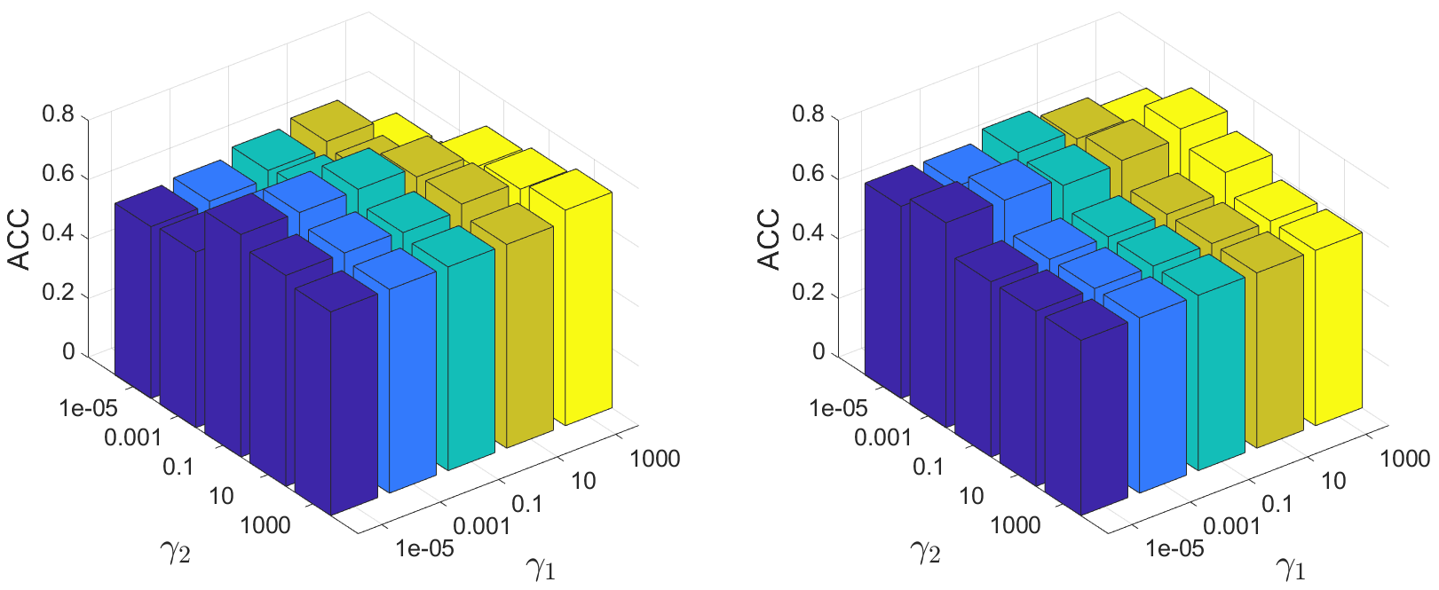
The loss function includes two balance parameters ${\gamma }_1$ and ${\gamma }_2$. To see their effect, we set ${\gamma }_1$, ${\gamma }_2$=[1e-5, 1e-3, 1e-1, 1e1, 1e3]. Their effect on clustering ACC of Cora and Washington is shown in Fig. 4. Our technique performs effectively for a wide range of parameters. The influence of ${\gamma }_2$ on performance is greater than ${\gamma }_1$, indicating the importance of cluster enhancement.

VI Ablation Study

To see the impact of our proposed adaptive GNN, we compare PFGC with different combinations. The $l$-th layer aggregation becomes:

$H_1^{(l)}$ $=(1-\mu )\left(I-{\displaystyle \frac{2}{3}}{\tilde{L}}_M\right)H_1^{(l-1)}{W}^{(l-1)}$ (33)

$+\mu \left({\displaystyle \frac{2}{3}}{\tilde{L}}_G\right)H_1^{(l-1)}{W}^{(l-1)},$

$H_2^{(l)}$ $=(1-\mu )U_1\mathrm{diag}\left({\left\{e^{1-{\lambda }_i^{(1)}}\right\}}_{i=1}^N\right)U_1^{\top }{H}_2^{(l-1)}{W}^{(l-1)}$

$+\mu U_2\mathrm{diag}\left({\left\{e^{{\lambda }_i^{(2)}}\right\}}_{i=1}^N\right)U_2^{\top }{H}_2^{(l-1)}{W}^{(l-1)},$

$H_3^{(l)}$ $=(1-\mu )\left(I-{\displaystyle \frac{2}{3}}{\tilde{L}}_M\right)H_3^{(l-1)}{W}^{(l-1)}$

$+\mu U_2\mathrm{diag}\left({\left\{e^{{\lambda }_i^{(2)}}\right\}}_{i=1}^N\right)U_2^{\top }{H}_3^{(l-1)}{W}^{(l-1)},$

which are marked as PFGC-1, PFGC-2, and PFGC-3, respectively. The results are shown in Table IV. PFGC achieves the best performance in all cases. PFGC exceeds PFGC-1 by a lot, since PFGC-1 only considers traditional local filters. Therefore, a global filter is beneficial in enhancing the quality of the representation. PFGC-3 achieves the worst performance in most cases, which is consistent with our theorem.

The homophily scores of the original graph and the constructed graphs are compared in Table V. It can be seen that the new graphs are highly homophilic or heterophilic. This shows that our graph restructuring method provides more rich information.

TABLE V: The homophily scores of restructured graphs.

	A	M	G
Cora	0.8100	0.8268$\uparrow$	0.1046
Citeseer	0.7355	0.7790$\uparrow$	0.0843
Pubmed	0.8024	0.8204$\uparrow$	0.2212
AMAP	0.8272	0.8836$\uparrow$	0.0653
UAT	0.6978	0.7005$\uparrow$	0.1872
Cornell	0.1227	0.4807$\uparrow$	0.2142
Wisconsin	0.1703	0.5059$\uparrow$	0.0360$\downarrow$
Washington	0.1530	0.5443$\uparrow$	0.0653$\downarrow$
Chameloen	0.2299	0.5382$\uparrow$	0.1742$\downarrow$
Squirrel	0.2234	0.4781$\uparrow$	0.1999$\downarrow$
Roman-Empire	0.0469	0.5000$\uparrow$	0.0223$\downarrow$

Figure 5: The results with masked features.

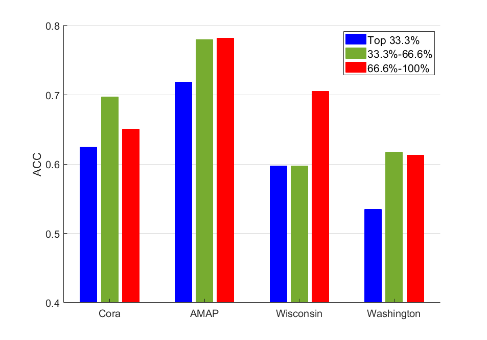
To test the squeeze-and-excitation block’s effect, we remove it and mark it as PFGC w/o SE. According to Table IV, there is a decrease in performance, indicating that the squeeze-and-excitation block improves the quality of the representation. We mask the final features $\tilde{H}$ according to the attention weights (i.e. $s$). We categorize it into three intervals: masking features of the top 33.3% (highest) weights, masking features from 33.3% to 66.6% weights, and the remaining 66.6% to 100%. After masking, we use K-means on the features to obtain the ACC results. As depicted in Fig. 5, when masking the most important features (top 33.3%), the performance suffers the most significant decrease. This suggests that the attention weights corresponding to the top features are crucial. For 33. 3%-66. 6% and 66. 6%-100%, their effect varies on different datasets. Therefore, our proposed squeeze-and-excitation block can successfully boost important features and thus enhance performance.

VII Conclusion

This study presents an innovative approach to graph clustering, specifically addressing the challenges posed by homophilic and heterophilic graph structures. One of our key contributions is the development of unsupervised strategies for graph restructuring, enabling the extraction of both homophilic and heterophilic information based on the commonality of graphs. Additionally, we design an adaptive GNN to better utilize the characteristics of restructured graphs. The incorporation of the squeeze-and-excitation block amplifies the significance of crucial features to further enhance the performance, making the first application of this concept to graph clustering. Theoretical and empirical results validate the effectiveness of our approach.

VIII Biography Section

Xuanting Xie received the B.Sc. degree in Software Engineering in 2021 and is currently studying for a Ph.D. degree with School of Computer Science and Engineering, the University of Electronic Science and Technology of China, Chengdu, China. His main research interests include graph leanring and clustering.

Erlin Pan received the B.Sc. degree in computer science and technology in 2021 and is currently studying for a M.S degree with School of Computer Science and Engineering, the University of Electronic Science and Technology of China, Chengdu, China.His main research interests include graph leanring, multi-view learning, and clustering.

Zhao Kang received the Ph.D. degree in computer science from Southern Illinois University Carbondale, Carbondale, IL, USA, in 2017. He is currently an Associate Professor with the School of Computer Science and Engineering, University of Electronic Science and Technology of China, Chengdu, China. He has published over 80 research papers in top-tier conferences and journals, including NeurIPS, AAAI, IJCAI, ICDE, CVPR, SIGKDD, ECCV, ICDM, CIKM, SDM, IEEE TRANSACTIONS ON CYBERNETICS, IEEE Transactions on Image Processing, IEEE Transactions on Knowledge and Data Engineering, and IEEE Transactions on Neural Networks and Learning Systems. His research interests are machine learning, pattern recognition, and data mining. Dr. Kang has been an AC/SPC/PC Member or a Reviewer for a number of top conferences, such as NeurIPS, ICLR, AAAI, IJCAI, CVPR, ICCV, MM, and ECCV. He regularly serves as a Reviewer for the Journal of Machine Learning Research, IEEE TRANSACTIONS ON PATTERN ANALYSIS AND MACHINE INTELLIGENCE, IEEE TRANSACTIONS ON NEURAL NETWORKS AND LEARNING SYSTEMS, IEEE TRANSACTIONS ON CYBERNETICS, IEEE TRANSACTIONS ON KNOWLEDGE AND DATA ENGINEERING, and IEEE TRANSACTIONS ON MULTIMEDIA.

Wenyu Chen received the Ph.D. degree in computer science from the University of Electronic Science and Technology of China, Chengdu, China, in 2009. He is currently a Professor with the School of Computer Science and Engineering, University of Electronic Science and Technology of China. His research work focuses on pattern recognition, natural language processing, and neural network.

Bingheng Li is currently a 2020 undergraduate student at the University of Electronic Science and Technology of China (UESTC). His research focuses on graph clustering and graph data mining.

References

- [1] C. Wang, S. Pan, G. Long, X. Zhu, and J. Jiang, “Mgae: Marginalized graph autoencoder for graph clustering,” in Proceedings of the 2017 ACM on Conference on Information and Knowledge Management, 2017., pp. 889–898.
- [2] S. Fortunato and D. Hric, “Community detection in networks: A user guide,” Physics reports, vol. 659, pp. 1–44, 2016.
- [3] X. Liu, “Incomplete multiple kernel alignment maximization for clustering,” IEEE Transactions on Pattern Analysis and Machine Intelligence, 2021.
- [4] X. Wang, P. Cui, J. Wang, J. Pei, W. Zhu, and S. Yang, “Community preserving network embedding,” in Proceedings of the AAAI conference on artificial intelligence, vol. 31, no. 1, 2017.
- [5] W. Cui, H. Zhou, H. Qu, P. C. Wong, and X. Li, “Geometry-based edge clustering for graph visualization,” IEEE transactions on visualization and computer graphics, vol. 14, no. 6, pp. 1277–1284, 2008.
- [6] F. Nie, J. Xue, W. Yu, and X. Li, “Fast clustering with anchor guidance,” IEEE Transactions on Pattern Analysis and Machine Intelligence, 2023.
- [7] B. Perozzi and L. Akoglu, “Discovering communities and anomalies in attributed graphs: Interactive visual exploration and summarization,” ACM Transactions on Knowledge Discovery from Data (TKDD), vol. 12, no. 2, pp. 1–40, 2018.
- [8] I. Cabreros, E. Abbe, and A. Tsirigos, “Detecting community structures in hi-c genomic data,” in 2016 Annual Conference on Information Science and Systems (CISS). IEEE, 2016, pp. 584–589.
- [9] A. Tsitsulin, J. Palowitch, B. Perozzi, and E. Müller, “Graph clustering with graph neural networks,” Journal of Machine Learning Research, vol. 24, no. 127, pp. 1–21, 2023.
- [10] F. Tian, B. Gao, Q. Cui, E. Chen, and T.-Y. Liu, “Learning deep representations for graph clustering,” in Proceedings of the AAAI Conference on Artificial Intelligence, no. 1, 2014.
- [11] S. Pan, R. Hu, S.-f. Fung, G. Long, J. Jiang, and C. Zhang, “Learning graph embedding with adversarial training methods,” IEEE transactions on cybernetics, vol. 50, no. 6, pp. 2475–2487, 2019.
- [12] J. Cheng, Q. Wang, Z. Tao, D. Xie, and Q. Gao, “Multi-view attribute graph convolution networks for clustering,” in Proceedings of the twenty-ninth international conference on international joint conferences on artificial intelligence, 2021, pp. 2973–2979.
- [13] X. Yang, Y. Liu, S. Zhou, S. Wang, W. Tu, Q. Zheng, X. Liu, L. Fang, and E. Zhu, “Cluster-guided contrastive graph clustering network,” in Proc. of AAAI, 2023.
- [14] Y. Liu, X. Yang, S. Zhou, X. Liu, S. Wang, K. Liang, W. Tu, and L. Li, “Simple contrastive graph clustering,” IEEE Transactions on Neural Networks and Learning Systems, 2023.
- [15] E. Pan and Z. Kang, “Multi-view contrastive graph clustering,” Advances in neural information processing systems, vol. 34, pp. 2148–2159, 2021.
- [16] Z. Kang, Z. Liu, S. Pan, and L. Tian, “Fine-grained attributed graph clustering,” in Proceedings of the 2022 SIAM International Conference on Data Mining (SDM). SIAM, 2022, pp. 370–378.
- [17] J. Zhu, Y. Yan, L. Zhao, M. Heimann, L. Akoglu, and D. Koutra, “Beyond homophily in graph neural networks: Current limitations and effective designs,” Advances in Neural Information Processing Systems, vol. 33, pp. 7793–7804, 2020.
- [18] ——, “Beyond homophily in graph neural networks: Current limitations and effective designs,” Advances in neural information processing systems, vol. 33, pp. 7793–7804, 2020.
- [19] H. Mao, Z. Chen, W. Jin, H. Han, Y. Ma, T. Zhao, N. Shah, and J. Tang, “Demystifying structural disparity in graph neural networks: Can one size fit all?” Advances in neural information processing systems, 2023.
- [20] Q. Li, Z. Han, and X.-M. Wu, “Deeper insights into graph convolutional networks for semi-supervised learning,” in Proceedings of the AAAI conference on artificial intelligence, vol. 32, no. 1, 2018.
- [21] X. Li, R. Zhu, Y. Cheng, C. Shan, S. Luo, D. Li, and W. Qian, “Finding global homophily in graph neural networks when meeting heterophily,” in International Conference on Machine Learning. PMLR, 2022.
- [22] D. Cartwright and F. Harary, “Structural balance: a generalization of heider’s theory.” Psychological review, vol. 63, no. 5, p. 277, 1956.
- [23] R. Lei, Z. Wang, Y. Li, B. Ding, and Z. Wei, “Evennet: Ignoring odd-hop neighbors improves robustness of graph neural networks,” Advances in Neural Information Processing Systems, 2022.
- [24] M. Welling and T. N. Kipf, “Semi-supervised classification with graph convolutional networks,” in J. International Conference on Learning Representations, 2017.
- [25] C. Wang, S. Pan, R. Hu, G. Long, J. Jiang, and C. Zhang, “Attributed graph clustering: A deep attentional embedding approach,” in Proceedings of the Twenty-Eighth International Joint Conference on Artificial Intelligence, 2019, pp. 3670–3676.
- [26] T. Wang, J. Wu, Z. Zhang, W. Zhou, G. Chen, and S. Liu, “Multi-scale graph attention subspace clustering network,” Neurocomputing, vol. 459, pp. 302–314, 2021.
- [27] H. Zhu and P. Koniusz, “Simple spectral graph convolution,” in 9th International Conference on Learning Representations, ICLR 2021, 2021.
- [28] Z. Lin and Z. Kang, “Graph filter-based multi-view attributed graph clustering.” in IJCAI, 2021, pp. 2723–2729.
- [29] Z. Lin, Z. Kang, L. Zhang, and L. Tian, “Multi-view attributed graph clustering,” IEEE Transactions on Knowledge and Data Engineering, vol. 35, no. 2, pp. 1872–1880, 2023.
- [30] S. Abu-El-Haija, B. Perozzi, A. Kapoor, N. Alipourfard, K. Lerman, H. Harutyunyan, G. Ver Steeg, and A. Galstyan, “Mixhop: Higher-order graph convolutional architectures via sparsified neighborhood mixing,” in International Conference on Machine Learning. PMLR, 2019, pp. 21–29.
- [31] S. Luan, C. Hua, Q. Lu, J. Zhu, M. Zhao, S. Zhang, X.-W. Chang, and D. Precup, “Is heterophily a real nightmare for graph neural networks to do node classification?” arXiv preprint arXiv:2109.05641, 2021.
- [32] D. Lim, F. Hohne, X. Li, S. L. Huang, V. Gupta, O. Bhalerao, and S. N. Lim, “Large scale learning on non-homophilous graphs: New benchmarks and strong simple methods,” Advances in Neural Information Processing Systems, vol. 34, pp. 20 887–20 902, 2021.
- [33] Z. Zhong, G. Gonzalez, D. Grattarola, and J. Pang, “Unsupervised network embedding beyond homophily,” IEEE Transactions on Machine Learning Research, 2022.
- [34] X. Xie, W. Chen, Z. Kang, and C. Peng, “Contrastive graph clustering with adaptive filter,” Expert Systems with Applications, vol. 219, p. 119645, 2023.
- [35] E. Pan and Z. Kang, “Beyond homophily: Reconstructing structure for graph-agnostic clustering,” in International conference on machine learning, 2023, pp. 1–10.
- [36] J. Xu, E. Dai, D. Luo, X. Zhang, and S. Wang, “Learning graph filters for spectral gnns via newton interpolation,” arXiv preprint arXiv:2310.10064, 2023.
- [37] J. Park, M. Lee, H. J. Chang, K. Lee, and J. Y. Choi, “Symmetric graph convolutional autoencoder for unsupervised graph representation learning,” in Proceedings of the IEEE/CVF international conference on computer vision, 2019, pp. 6519–6528.
- [38] Z. Hou, X. Liu, Y. Dong, C. Wang, J. Tang et al., “Graphmae: Self-supervised masked graph autoencoders,” SIGKDD, 2022.
- [39] B. Chamberlain, J. Rowbottom, M. I. Gorinova, M. Bronstein, S. Webb, and E. Rossi, “Grand: Graph neural diffusion,” in International Conference on Machine Learning. PMLR, 2021, pp. 1407–1418.
- [40] Z. Yang, W. Cohen, and R. Salakhudinov, “Revisiting semi-supervised learning with graph embeddings,” in International Conference on Machine Learning. PMLR, 2016, pp. 40–48.
- [41] Y. Liu, W. Tu, S. Zhou, X. Liu, L. Song, X. Yang, and E. Zhu, “Deep graph clustering via dual correlation reduction,” in Proceedings of the AAAI Conference on Artificial Intelligence, vol. 36, no. 7, 2022, pp. 7603–7611.
- [42] N. Mrabah, M. Bouguessa, M. F. Touati, and R. Ksantini, “Rethinking graph auto-encoder models for attributed graph clustering,” IEEE Transactions on Knowledge and Data Engineering, 2022.
- [43] B. Rozemberczki, C. Allen, and R. Sarkar, “Multi-scale attributed node embedding,” Journal of Complex Networks, vol. 9, no. 2, p. cnab014, 2021.
- [44] O. Platonov, D. Kuznedelev, M. Diskin, A. Babenko, and L. Prokhorenkova, “A critical look at the evaluation of gnns under heterophily: are we really making progress?” in The Eleventh International Conference on Learning Representations, 2023.
- [45] H. Pei, B. Wei, K. C.-C. Chang, Y. Lei, and B. Yang, “Geom-gcn: Geometric graph convolutional networks,” in International Conference on Learning Representations, 2020.
- [46] H. Zhu and P. Koniusz, “Simple spectral graph convolution,” in 9th International Conference on Learning Representations, ICLR 2021,, 2021.
- [47] P. Zhu, J. Li, Y. Wang, B. Xiao, S. Zhao, and Q. Hu, “Collaborative decision-reinforced self-supervision for attributed graph clustering,” IEEE Transactions on Neural Networks and Learning Systems, 2022.
- [48] P.-Y. Huang, R. Frederking et al., “Rwr-gae: Random walk regularization for graph auto encoders,” arXiv preprint arXiv:1908.04003, 2019.
- [49] K. Hassani and A. H. Khasahmadi, “Contrastive multi-view representation learning on graphs,” in International Conference on Machine Learning. PMLR, 2020, pp. 4116–4126.
- [50] D. Bo, X. Wang, C. Shi, M. Zhu, E. Lu, and P. Cui, “Structural deep clustering network,” in Proceedings of The Web Conference 2020, 2020, pp. 1400–1410.
- [51] W. Tu, S. Zhou, X. Liu, X. Guo, Z. Cai, E. Zhu, and J. Cheng, “Deep fusion clustering network,” in Proceedings of the AAAI Conference on Artificial Intelligence, vol. 35, no. 11, 2021, pp. 9978–9987.
- [52] Y. Liu, W. Tu, S. Zhou, X. Liu, L. Song, X. Yang, and E. Zhu, “Deep graph clustering via dual correlation reduction,” in Proc. of AAAI, 2022.
- [53] G. Cui, J. Zhou, C. Yang, and Z. Liu, “Adaptive graph encoder for attributed graph embedding,” in Proceedings of the 26th ACM SIGKDD International Conference on Knowledge Discovery & Data Mining, 2020, pp. 976–985.