Learning Transferable Time Series Classifier with Cross-Domain Pre-training from Language Model

Abstract.

Advancements in self-supervised pre-training (SSL) have significantly advanced the field of learning transferable time series representations, which can be very useful in enhancing the downstream task. Despite being effective, we notice that most existing works struggle to achieve cross-domain SSL pre-training, missing valuable opportunities to integrate patterns and features from different domains. The main challenge lies in the significant differences in the characteristics of time-series data across different domains, such as variations in the number of channels and temporal resolution scales. To address this challenge, we propose CrossTimeNet, a novel cross-domain SSL learning framework to learn transferable knowledge from various domains to largely benefit the target downstream task. One of the key characteristics of CrossTimeNet is the newly designed time series tokenization module, which could effectively convert the raw time series into a sequence of discrete tokens based on a reconstruction optimization process. Besides, we highlight that predicting a high proportion of corrupted tokens can be very helpful for extracting informative patterns across different domains during SSL pre-training, which has been largely overlooked in past years. Furthermore, unlike previous works, our work treats the pre-training language model (PLM) as the initialization of the encoder network, investigating the feasibility of transferring the knowledge learned by the PLM to the time series area. Through these efforts, the path to cross-domain pre-training of a generic time series model can be effectively paved. We conduct extensive experiments in a real-world scenario across various time series classification domains. The experimental results clearly confirm CrossTimeNet’s superior performance. We hope the CrossTimeNet will inspire further research in developing universal time series representations. Our codes are publicly available.

1. Introduction

Time series classification (TSC) (Ismail Fawaz et al., 2019; Shifaz et al., 2020) is a fundamental challenge task in data science ranging various applications, from healthcare diagnostics (e.g., physiological signals) to industrial monitoring ((e.g., sensors and Internet of Things (IoT)). Recent works (Zheng et al., 2014; Liu et al., 2021, 2024a) show that deep learning methods have significantly resolved this area, due to their offering unparalleled scalability and the ability to model complex, nonlinear relationships within domain-specific data compared to classical models.

However, we notice that directly applying deep learning-based models does not always yield satisfactory results in real-world applications. The primary issue is that most advanced models, such as Transformer-based networks (Vaswani et al., 2017), are data-intensive, necessitating the collection of extensive labeled training data from the specific application scenario. To overcome this limitation, a significant amount of recent research proposes utilizing self-supervised learning (SSL) over vast amounts of unlabeled time series data. The core idea is that this type of approach can leverage the initial foundation provided by the pre-training stage, thereby reducing the need for extensive training resources during the model deployment phase. Furthermore, pre-trained models can enhance performance by discerning valuable patterns within the data from the extensive pre-training datasets. Recently, various strategies have been explored to extract general-purpose features from different angles, including methods like contrastive learning algorithms (Yue et al., 2022) and denoising autoencoder models (Zerveas et al., 2021; Cheng et al., 2023b).

Though effective, we notice that these current methods often assume that self-supervised training is confined within the same domain, overlooking the importance of learning transferable knowledge from other domains. Indeed, previous work, as highlighted in (Yang et al., 2021), has demonstrated that a well-trained acoustic model can serve as a powerful feature extractor for time series analysis. From our perspective, cross-domain self-supervised pre-training could naturally bring several advantages. Firstly, cross-domain learning promotes the discovery of latent correlations and patterns across different domains, enriching the model’s understanding and improving its predictive capabilities. Secondly, it enables the leveraging of vast amounts of unlabeled data across different domains, facilitating the learning of generalized features that are robust and transferable. This approach helps in overcoming the limitations posed by data scarcity in specific domains by utilizing the underlying patterns present in diverse datasets. Thirdly, cross-domain pre-training enhances model adaptability, allowing it to perform well across a variety of tasks without the need for extensive domain-specific tuning. For instance, by training a large language model to follow various types of human instructions (Ouyang et al., 2022), the language model can perform well even in zero-shot tasks.

Motivated by the analysis above, we decide to explore a promising yet under-explored SSL pre-training paradigm aimed at enhancing time series representation, specifically, pre-training across multiple domains. This endeavor is notably challenging, as different types of datasets typically possess distinct attributes and adhere to diverse distributions. Such discrepancies complicate the task of representing various domains within a unified representation space. For instance, considering the widely used time series data in physiological signals alone, we encounter a broad spectrum of types such as electrocardiograms (ECG), electroencephalograms (EEG), among others. Unlike textual data, these cross-domain time series datasets vary significantly in terms of the number of channels, sampling rates, and even the unique characteristics inherent to each domain. Therefore, devising a method to unify instances from different domains is crucial for constructing a cohesive pre-trained model. In addition to the challenges posed by the cross-domain scenario, we are also keen on addressing two specific aspects: the design of the SSL optimization objective and the selection of an appropriate encoder backbone network for representation learning. Regarding the former, we observe that most recent works (Zhang et al., 2023) predominantly focus on SSL optimization over raw time series data, employing instance-level contrastive learning optimization. As for the latter, current research tends to rely on either convolutional (Yue et al., 2022) or Transformer-based networks (Cheng et al., 2023b), typically initialized in a random manner, as the encoders. In our view, the above design might not well accomplish the cross domain pre-training optimization.

In this work, we propose CrossTimeNet, a novel framework designed for cross-domain self-supervised pre-training on time series data. To accommodate the diverse characteristics of time series data across various domains, we provide a carefully designed tokenizer that can convert continuous time series into discrete tokens through a reconstruction optimization process. This tokenizer enables each segment of the raw time series to be assigned its own identity code, effectively bridging the gap caused by data discrepancies across domains. Within CrossTimeNet, we emphasize two key insights. Firstly, we find that predicting a higher proportion of corrupted time series tokens is beneficial for learning more informative patterns within the data. Secondly, we unexpectedly discover that utilizing a pre-trained language model as the encoder backbone network is highly effective for extracting time series representations. Leveraging these strategies allows us to develop a universal pre-trained time series model that distills various types of knowledge and patterns from different domains. To assess the effectiveness of CrossTimeNet, we conduct comprehensive experiments on time series classification tasks using several real-world datasets. The experimental results unequivocally affirm the superiority of our CrossTimeNet from multiple angles. We hope that CrossTimeNet will inspire further research in the quest for developing general-purpose time series representation models.

2. Related Work

The related research primarily falls into two categories: time Series classification and self-supervised time series representation.

2.1. Time Series Classification

Time series classification (TSC) has garnered significant attention from researchers in recent years (Middlehurst et al., 2023; Shifaz et al., 2020). Through an extensive review of the literature, these contributions can be broadly categorized into four types approaches. Distance-based methods form the bedrock of traditional TSC, primarily leveraging similarity measures to classify time series. The quintessential example is the dynamic time warping (DTW) algorithm, when combined with a nearest neighbor classifier (NN-DTW) (Ding et al., 2008). Interval-based approaches focus on extracting features from specific intervals of the time series. Time series forest (TSF) (Deng et al., 2013) is a notable method in this category, employing random interval selection and summary statistics to capture local patterns. Shapelet-based (Ye and Keogh, 2009) methods revolve around identifying sub-sequences (shapelets) that are predictive of a time series class. The learning shapelets (Grabocka et al., 2014) algorithm is a prime work, providing an automated process for shapelet discovery directly from the data. Dictionary-based techniques involve transforming time series into symbolic representations and then analyzing the frequency of these symbolic patterns. One of the seminal works in this area is the Symbolic Aggregate approXimation (SAX) (Lin et al., 2007), which enables a bag-of-words type model for TSC. This approach has been further extended by methods such as Bag of Patterns (BOP) (Lin et al., 2012) and symbolic aggregate approXimation - vector space model (SAX-VSM) (Senin and Malinchik, 2013). Although effective in some scenarios, these methods excel in handling temporal distortions but can be computationally intensive for large datasets. In contrast, Deep Learning-based methods have surged in popularity due to their ability to efficiently learn complex features from raw time series data (Zhang et al., 2020). Convolutional neural networks (CNNs) (Zheng et al., 2014; Wang et al., 2017; Cheng et al., 2024), and Self-attention based Transformer architectures (Liu et al., 2021; Cheng et al., 2023a; Wen et al., 2022) have been at the forefront of this wave, showcasing remarkable performance across diverse TSC tasks. These deep learning methods benefit from the ability to model long-term dependencies and hierarchical feature representations without the need for manual feature engineering (Liu et al., 2024b; Christ et al., 2018). Despite the profound nonlinear modeling capabilities of deep neural networks and their advantage of obviating the need for manual feature engineering—thereby facilitating the learning of more complex temporal features for effective classification—their major drawback lies in their voracious data appetite. These models necessitate extensive labeled training sets, without which they are prone to overfitting.

2.2. Self-supervised Time Series Representation

In response to the data-hungry challenge of deep learning based methods, a considerable amount of recent research (Zhang et al., 2023) has been centered around self-supervised learning for time series representation. Upon reviewing and synthesizing the current body of work in this area, self-supervised pre-training efforts for time series data can be broadly categorized into the following approaches: encoder-decoder models, contrastive learning-based techniques, and denoising auto-encoder based. Encoder-decoder models: The primary philosophy behind this category is to leverage an encoder to transform input time series data into a latent representation, which is then reconstructed back to the original input (or some variant of it) by a decoder. This approach encourages the model to capture essential temporal dynamics and dependencies in the data. Contrastive learning-based techniques: This paradigm focuses on learning representations by distinguishing between similar (positive) and dissimilar (negative) pairs of time series segments (Oord et al., 2018). Techniques such as TNC (Tonekaboni et al., 2021), TS-TCC (Eldele et al., 2021), and TS2Vec (Yue et al., 2022) fall under this umbrella, each employing unique mechanisms to define and utilize positive and negative samples for training robust time series representations. Denoising auto-encoder based approaches: Methods like TST (Zerveas et al., 2021) and TimeMAE (Cheng et al., 2023b) adopt a reconstructive strategy, where the model is trained to predict missing parts of the input time series or reconstruct the series from distorted versions.

Figure 1. Overview of CrossTimeNet: a unified framework for self-supervised pre-training of cross-domain time series data.

3. Preliminaries

First, we introduce the studied problem, used notation and concepts. Then, we briefly present the relative models in our work.

Self-supervised Pre-training Across Domains

In this work, our primary goal is to create a unified self-supervised pre-training framework that can efficiently handle time series data from a wide range of scenarios, each referred to as a ”domain.” These domains encompass distinct characteristics and patterns within the time series data. To tackle the challenge of self-supervised pre-training across multiple domains, we introduce $𝒟={𝒟}_1,{𝒟}_2,\mathrm{\dots },{𝒟}_N$, a collection of datasets representing $N$ distinct domains. Each domain dataset $𝒟n$ comprises unlabeled time series data ${𝐱}_i^n$, with ${𝐱}_i^n=[x_{i1}^n,x_{i2}^n,\mathrm{\dots },x_{iT}^n]$ representing the $i$-th time series instance in the $n$-th domain, consisting of $T$ time points. The key challenge lies in leveraging the vast, unlabeled data across these varied domains to train a versatile pre-trained model $𝒫$. This model is designed to capture universal features and patterns inherent in time series data, going beyond the specific characteristics of individual domains. The self-supervised learning approach enables the model to uncover and utilize the intrinsic structure of the data without depending on explicit class labels, thereby tapping into the unexploited wealth of unlabeled data across different domains.

Once the pre-trained model $𝒫$ is established, it can be fine-tuned for corresponding downstream tasks, denoted as $𝒯={𝒯}_1,{𝒯}_2,\mathrm{\dots },{𝒯}_N$. These tasks may either fall within the same domains as those used in the pre-training phase or extend across different domains, showcasing the adaptability and transferability of the representations learned by the model. The ultimate aim is to employ the pre-trained model $𝒫$ to boost the performance and generalization capabilities of models ${ℱ}_n$ designated for time series classification tasks within specific domains. Each model ${ℱ}_n:{𝐱}_i^n\mapsto y_i^n$ is responsible for mapping a time series to its accurate class label within the respective task domain ${𝒯}_n$, thereby enhancing the efficacy of time series classification across a broad spectrum of domains.

Pre-trained Language Model

Recently, pre-trained language models (PLM) (Devlin et al., 2018) have revolutionized the field of natural language processing (NLP) by providing a powerful framework for learning rich linguistic representations from vast amounts of textual data. At their core, PLM are models that have been trained on a large corpus of text in a self-supervised manner, meaning they learn to predict parts of the text based on other parts, without the need for explicit annotations or labels. This training approach allows them to capture a wide range of language phenomena and contextual nuances, making them highly versatile and effective for various NLP tasks. The typical processing pipeline for text with a PLM begins with tokenization, where the input text is broken down into manageable pieces, often words or subwords, known as tokens. These tokens are then fed into a designed neural network, e.g., Transformers (Vaswani et al., 2017), which processes them to extract dynamic contextual features. Due to the powerful capacity shown in PLM, it nearly become a default paradigm in the NLP domain.

4. The Proposed CrossTimeNet

To begin with, we introduce the methodological framework of CrossTimeNet, followed by a detailed explanation of the methodological details.

4.1. Overview of Model Architecture

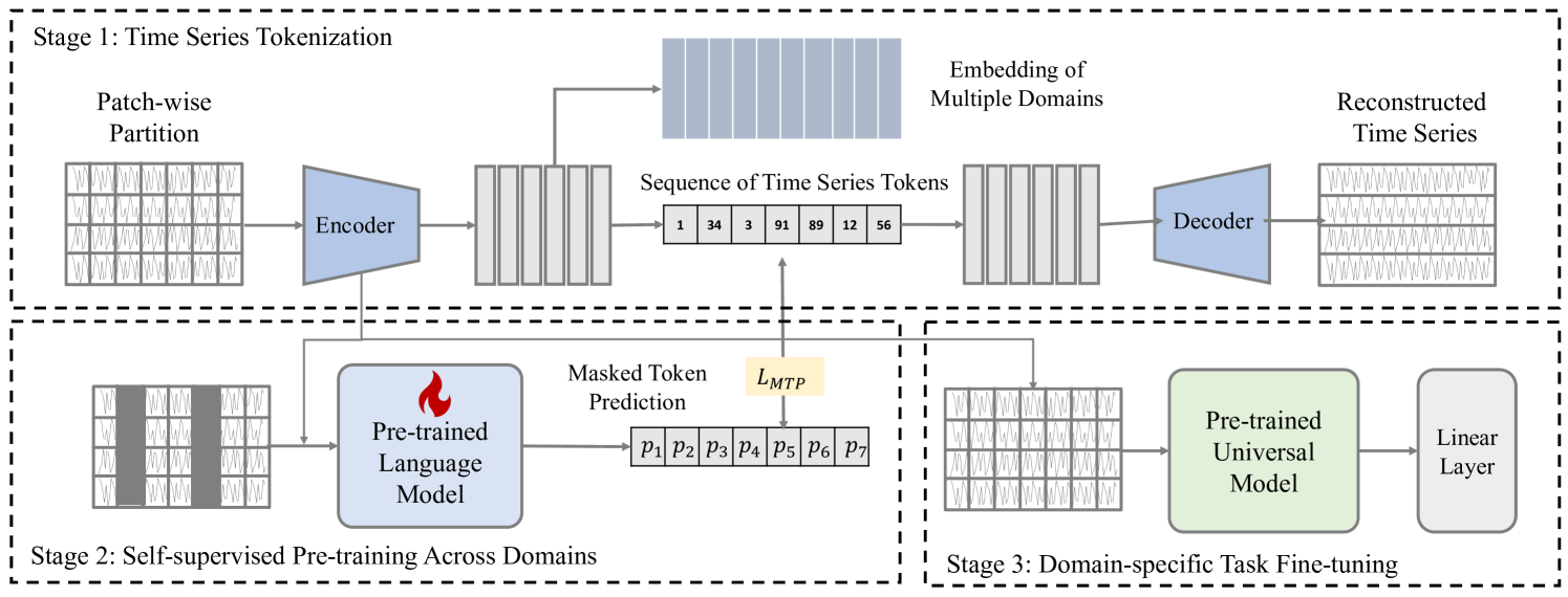
As depicted in Figure 1, the CrossTimeNet encompasses three core components: (a) time series tokenization, (b) self-supervised pre-training across domains, and (c) domain-specific task fine-tuning. During time series tokenization, a tailor-made tokenizer converts continuous time series data into discrete tokens, establishing a uniform representation suitable for cross-domain application. Following this, the self-supervised pre-training phase employs a bidirectional token prediction task—where random tokens are masked—to compel the model to deduce missing information, thereby learning potent representations of the time series data. Finally, in the downstream task fine-tuning stage, the model undergoes specific adjustments to excel in domain-related tasks, such as classification, harnessing the extensive knowledge gained from pre-training process. This fine-tuning is meticulously carried out to ensure the model’s proficiency in specialized tasks while retaining the extensive insights from its earlier cross-domain exposure.

4.2. Time Series Tokenization

Time series data poses distinct challenges for cross-domain analysis due to its inherent variability in structure, unlike more consistent modalities like text and vision. Variations in channel numbers, physical phenomena representation, and temporal resolutions across domains complicate the development of universally applicable pre-trained models. For example, the simplicity of financial time series contrasts sharply with the complexity of multichannel EEG data. Addressing this, one may wonder that channel-independent modeling (Han et al., 2023) emerges as a promising approach, treating each channel as separate to bridge differences between datasets. However, this method may neglect crucial inter-channel dependencies, which are especially vital in fields like healthcare, where understanding the relationships between different physiological signals is key. This oversight could result in a less comprehensive interpretation of the data, highlighting the need for models that can balance generalization with the retention of critical inter-channel information.

In this work, we decide to adopt a direct yet under-explored path - time series discretation during pre-training time series representations. The main idea is to transform the time series into a format that maintains the essential inter-channel relationships while still accommodating the diverse characteristics of data across domains. This discretization not only standardizes the input data but also preserves the rich, multi-faceted information that is crucial for the subsequent stages of self-supervised pre-training and downstream task fine-tuning. Through this approach, we endeavor to construct a robust and versatile pre-trained model, one that harnesses the full spectrum of information within multi-domain time series data while overcoming the inherent challenges posed by their variability. Although some previous works have explored the discretization of time series, including SAX (Lin et al., 2007) and SFA (Schäfer and Högqvist, 2012; Schäfer, 2015), these methods suffer from a significant drawback: they are computationally expensive. In addition, these methods exhibit significant limitations when applied to self-supervised pre-training of time series data. They struggle to compress complex temporal sequences effectively, often resulting in substantial information loss. Moreover, these techniques typically require manual tuning, which can introduce subjectivity and limit their scalability.

In light of this, inspired by the success of image compression (Van Den Oord et al., 2017), we employ a auto-encoder framework to achieve efficient time series compression, referred to as time series tokenizer. The tokenizer involves several steps. First, we transform the time series along the time dimension into sequence patches. Formally, for a given time series instance ${𝐱}^{𝐧}=[x_1^n,x_2^n,\mathrm{\dots },x_T^n]$ in the $n$-th domain, it is first segmented into $n$ non-overlap patches ${𝐬}_1,{𝐬}_2,\mathrm{\dots },{𝐬}_L$, where each patch ${𝐬}_n$ contains a subset of consecutive time points from the original series. These patches are then fed into the auto-encoder architecture. In the following sections, we omit the mathematical notation for domains for brevity.

In this work, we propose to map each patch ${𝐬}_l$ to a latent representation ${𝐳}_n$. The TCN architecture (Oord et al., 2016) is chosen for its ability to capture long-range dependencies and for its efficient computation:

(1) $${𝐳}_l=\text{Encoder}\text{TCN}({𝐬}_l).$$

Following the encoding, the vector quantization step occurs. Here, each latent representation ${𝐳}_l$ is mapped to the nearest vector in a learned codebook $𝐞=[{𝐞}_1,{𝐞}_2,\mathrm{\dots },{𝐞}_K]$, where $K$ is the size of the codebook. This mapping is given by:

(2) $${𝐳}_l^q=\text{argmin}{𝐞}_k\in 𝐞{|{𝐳}_l-{𝐞}_k|}^2.$$

where ${𝐳}_l^q$ denote the assigned code selected from codebook. The decoder then reconstructs the time series from the quantized vectors, aiming to minimize the reconstruction error and thus preserve as much of the original sequence information as possible:

(3) $$\widehat{𝐱}={\text{Decoder}}_{\text{TCN}}({𝐳}^q).$$

By using this auto-encoder framework with TCNs, we can effectively compress the time series into a discrete representation that is amenable to self-supervised learning tasks while preserving the critical temporal dynamics that are essential for downstream applications. Our optimization process aligns with the approach used in the prior work of VQ-VAE (Oord et al., 2016), where it is particularly noteworthy that the nearest-neighbor selection process is non-differentiable, leading to challenges in gradient derivation. Due to space constraints in this paper, we omit a detailed discussion, and interested readers may refer to the relevant literature for further information. The novel contribution of our work is that a novel time series discretization is implemented, which is greatly different from previous works.

4.3. Self-supervised Pre-training

4.3.1. Masked Token Prediction

In this subsection, we introduce the cross-domain self-supervised optimization objectives. In the realm of time series analysis, in our view, an ideal self-supervised optimization task should fulfill two pivotal objectives. Firstly, it must be capable of learning rich contextual information (Kong and Zhang, 2023), ensuring that each position within the series is accurately represented (Objective 1). This requirement stems from the inherent sequential nature of time series data, where the understanding of a given point is significantly enhanced by its preceding and succeeding elements. Secondly, maintain a certain level abstraction of the predicted targets in the self-supervised optimization loss can be beneficial to improving the transferablility of pre-trained models (Objective 2). This idea is also consistent in (Kostelich and Schreiber, 1993), which think that directly formulating self-supervised signals in raw space would largely restrict the capacity of the model due to the noisy and unbound properties. Thirdly, the optimization challenge posed by the self-supervised pre-training should be sufficiently challenge (He et al., 2022) (Objective 3). This difficult is crucial as it compels the model to learn a more profound and comprehensive set of knowledge, which, in turn, can be leveraged to augment the performance on downstream tasks.

Given these considerations, our approach in this paper is to design a self-supervised optimization task characterized by a relatively high ratio (more than 30%) of masked token prediction. This design choice is predicated on the hypothesis that by obscuring a substantial portion of the input data, the model is compelled to infer the masked information based solely on the context provided by the visible data points. Precisely, let $ℳ$ denotes the set of masked positions within the time series data. Suppose the predicted corresponding to the masked inputs are $s_l$, with $l\in ℳ$. Formally, the reconstruction self-supervised optimization goal ${ℒ}_{MTP}$ can be described as follows:

(4) $${ℒ}_{MTP}=-\sum _{l\in ℳ}\log p(s_l|{𝐱}_{\backslash ℳ};\mathrm{\Theta }),$$

where ${𝐱}_{\backslash ℳ}$ signifies the sequence with the masked tokens removed, and $\mathrm{\Theta }$ encapsulates the model parameters. This task not only encourages the model to learn robust representations by leveraging bidirectional context but also ensures that the optimization challenge is sufficiently demanding to facilitate the acquisition of valuable knowledge for downstream applications.

4.3.2. Pre-trained Language Model as Encoders

A comprehensive review of the extant literature reveals that the backbone networks in the domain of time series self-supervised learning predominantly harness either convolutional neural networks (e.g., TCN in (Oord et al., 2016)) or Transformer networks in (Vaswani et al., 2017). Given our endeavor to explore cross-domain self-supervised pre-training, it is imperative that the chosen backbone architecture exhibits a high degree of universality to cater to diverse domains effectively. Drawing inspirations from cognitive science literature (Dehaene-Lambertz, 2017), which posits that human learning is not initiated from a tabula rasa but rather resembles a form of pre-trained network, we ventured to adopt a similar paradigm for our backbone network. This approach aligns with the concept that infants’ brains, though not fully developed, are equipped with a rudimentary but potent learning framework right from birth. In this vein, our experimental forays led us to an intriguing discovery: employing a pre-trained language model as the backbone network significantly amplifies performance, marking a substantial leap in achieving superior outcomes in time series analysis. This finding is particularly noteworthy as it challenges the conventional neglect of such a potentially efficacious setting in prior research.

Specifically, we draw upon the network architecture of BERT (Devlin et al., 2018), renowned for its masked language modeling (MLM) and next sentence prediction (NSP) tasks, to serve as the foundational base model for our network initialization. This choice is predicated on BERT’s proven versatility and robustness in capturing contextual dependencies, making it an ideal candidate for our cross-domain self-supervised learning framework. The adoption of a pre-trained language model as the backbone, therefore, represents a novel and promising avenue in the realm of time series analysis, setting the stage for further exploration and validation in future work.

Upon integrating a language model, we encountered the challenge of encoding time series tokens within the BERT network. Although the codebook embedding from tokenizer could be directly utilized, discrepancies in the embedding size and potential gaps in the representational space compared to BERT’s word embeddings were apparent. To address this, we employed a word mapping mechanism (Kao and Lee, 2021), randomly assigning each token a corresponding word selected from BERT’s vocabulary. This approach effectively resolved the encoding issues of time series tokens, ensuring seamless integration with the language model framework. It should be noted that we provide a detailed comparison of the differences in word mapping to illustrate that the specific impact as shown in Table 10 presented in Appendix C.3.

4.4. Downstream Task Adaptation

Upon the completion of cross-domain self-supervised pre-training, we have successfully developed a versatile foundation model. To assess the efficacy of the pre-trained model, it is crucial to employ rigorous evaluation techniques. While acknowledging the plethora of transfer learning strategies available, such as Adapter-based methods among others (Hu et al., 2021; Fu et al., 2023), it is pertinent to note that these are beyond the scope of our current investigation and are earmarked for future research endeavors. In this work, we adopt two classical evaluation paradigms within the self-supervised learning framework: linear evaluation and full fine-tuning. In linear evaluation, we freeze the weights of the pre-trained model, preserving the learned representations. A linear classifier is then added on top of the model. This classifier is the only component that is trained on the downstream task dataset. This approach allows us to evaluate the quality and transferability of the features learned during the self-supervised pre-training phase without modifying the underlying representations. Linear evaluation is particularly useful for assessing the generalizability of the pre-trained model across different domains with minimal computational cost. Contrary to linear evaluation, full fine-tuning involves adjusting the entire model, including both the pre-trained layers and the newly added task-specific layers. This approach allows the model to fine-tune the learned representations in conjunction with learning the downstream task, potentially leading to higher performance on the target task. Full fine-tuning is more computationally intensive but can result in a model that is more closely tailored to the specifics of the target task, leveraging both the generic representations learned during pre-training and the specific nuances of the new task.

Table 1. Main performance comparison of our methods and compared baselines, in terms of two types of fine-tuning strategy. The ‘N/A’ placeholder denotes instances where the model’s accuracy is effectively zero the threshold of measurement precision.

Fine-tuning Strategies	Models	HAR		EEG		ECG
		Accuracy	F1 Score	Accuracy	F1 Score	Accuracy	F1 Score
Full Fine-tuning	TST-Zero	0.9121	0.9120	0.7938	0.5211	0.1808	0.3861
	TST	0.9203	0.9203	0.8086	0.5516	0.2206	0.3317
	TimeMAE	0.9294	0.9284	0.8248	0.5865	0.2546	0.3834
	TNC	0.8961	0.8951	0.7603	0.4457	0.2081	0.3310
	TS-TCC	0.8832	0.8815	0.7291	0.4347	0.1778	0.3780
	TS2Vec	0.8968	0.8957	0.7565	0.4449	0.1302	0.2064
	CrossTimeNet-w/o-SSL	0.8550	0.8520	0.7929	0.5426	0.2134	0.3246
	CrossTimeNet	0.9335	0.9347	0.8541	0.6402	0.4378	0.6278
Linear Evaluation	TST-Zero	0.7211	0.7120	0.5538	0.2236	N/A	N/A
	TST	0.8337	0.8300	0.6664	0.3553	0.0133	0.0234
	TimeMAE	0.8918	0.8912	0.7459	0.4543	0.0510	0.0810
	TNC	0.7713	0.7652	0.7347	0.4172	0.0108	0.0140
	TS-TCC	0.7520	0.7504	0.5623	0.2281	N/A	N/A
	TS2Vec	0.7241	0.7159	0.6945	0.3762	N/A	N/A
	CrossTimeNet-w/o-SSL	0.7861	0.7800	0.7333	0.4504	0.0531	0.0818
	CrossTimeNet	0.9146	0.9148	0.8381	0.6072	0.2134	0.3148

5. Experiments

5.1. Experimental Setup

Several prevalent real-world datasets for evaluating the effectiveness of our works, including HAR, ECG, EEG. Noted that each data represent a distinct domain of time series classification. Please refer to the Appendix A for the detailed dataset setting. To ascertain the effectiveness of our proposed CrossTimeNet, we conducted a series of comparative analyses against a spectrum of prevailing self-supervised baselines. These baselines encompass three primary categories: denoising auto-encoder based methods, including TST (Zerveas et al., 2021) and TimeMAE (Cheng et al., 2023b); contrastive Learning approaches such as TNC (Tonekaboni et al., 2021), TS-TCC (Eldele et al., 2021), and TS2Vec (Yue et al., 2022). Please refer to the Appendix B for the detailed baselines and experimental settings. In this work, we employ Accuracy and F1 Score as measurement metrics.

Table 2. Performance comparison of model variants w.r.t network parameter settings equipped with different configuration.

Fine-tuning Strategies	Models	HAR		EEG		ECG
		Accuracy	F1 Score	Accuracy	F1 Score	Accuracy	F1 Score
Full Fine-tuning	RandInit Transformer	0.9111	0.9109	0.8339	0.5984	0.3408	0.4826
	RandInit BERT	0.8489	0.8453	0.7621	0.4859	0.1451	0.2338
	Pre-trained BERT	0.9305	0.9305	0.8541	0.6327	0.4287	0.6161

5.2. Results and Analysis

5.2.1. Downstream Classification Results

Table 1 presents a comprehensive performance comparison of various models. The highlighted results show that the CrossTimeNet model outperforms all other compared baselines in every category and evaluation manner, indicating its superior ability in handling time-series data across these diverse domains. One notable observation is the significant performance gap between Full Fine-tuning and Linear Evaluation methods, particularly for the CrossTimeNet model, which maintains its lead in both evaluation strategies but with a noticeable drop in performance in the Linear Evaluation, especially in the ECG dataset. This drop might be attributed to the complexity and intrinsic variability of ECG data, which could be more challenging to capture with linear models without fine-tuning all layers. Another point of interest is the variable performance of models across different datasets. For instance, TimeMAE shows strong results in HAR under Full Fine-tuning but is not applied to EEG and ECG datasets, possibly indicating its specialization or limitations in handling specific types of time-series data. The relatively low performance of all models on the ECG dataset, particularly in the Linear Evaluation, highlights the challenges in ECG signal analysis, which may be due to the complexity of the signals, the need for more nuanced feature extraction, or the limitations of Linear Evaluation methods in capturing the intricate patterns within ECG data. To sum up, the CrossTimeNet model demonstrates a robust capability across different types of time-series data, with its performance indicating a strong generalization ability. However, the performance variation across different datasets and evaluation methods underscores the importance of model selection based on the specific characteristics of the data and the task at hand.

5.2.2. Study of Using PLM as Encoders

Table 2 provides a performance comparison of different network configurations. The model variants of CrossTimeNet include a randomly initialized BERT (RandInit BERT), and a Pre-trained BERT. Across all datasets and evaluation methods, the results reinforce the critical role of pre-training in enhancing model performance. Pre-trained BERT models, with their deep, complex architectures, are particularly effective, outperforming simple Transformer and RandInit BERT without pre-training. This suggests that the combination of a powerful architecture and extensive pre-training is key to achieving high accuracy and F1 scores in tasks involving complex time-series data like HAR, EEG, and ECG analysis. Furthermore, the Pre-trained BERT configuration demonstrates superior performance, underscoring the effectiveness of leveraging pre-trained models for time-series classification tasks. The RandInit BERT, despite sharing a similar structural architecture with the Pre-trained BERT, shows significantly lower performance. This suggests that the architecture alone is not sufficient to achieve high performance without the rich, pre-learned representations that come from pre-training on large datasets.

Table 3. Performance of CrossTimeNet with various PLM configurations measured by full fine-tuning.

Fine-tuning Strategies	Settings	HAR		EEG		ECG
		Accuracy	F1 Score	Accuracy	F1 Score	Accuracy	F1 Score
Full Fine-tuning	RoBERTa	0.9338	0.9350	0.8494	0.6242	0.4345	0.6144
	BERT-Small	0.9291	0.9298	0.8431	0.6205	0.3770	0.5556
	BERT-Base	0.9335	0.9347	0.8541	0.6402	0.4378	0.6278
	BERT-Large	0.9406	0.9417	0.8614	0.6466	0.4502	0.6190

Table 4. Results of model variants by employing BERT and GPT2 as initialization parameters of encoder network.

Fine-tuning Strategies	Models	HAR		EEG		ECG
		Accuracy	F1 Score	Accuracy	F1 Score	Accuracy	F1 Score
Full Fine-tuning	Transformer with AR	0.8568	0.8534	0.8001	0.5472	0.2604	0.3978
	Transformer with MTP	0.7618	0.7527	0.7959	0.5234	0.1650	0.2303
	GPT2-as-Encoder with AR	0.9258	0.9261	0.8353	0.5947	0.4101	0.5949
	BERT-as-Encoder with MTP	0.9335	0.9347	0.8541	0.6402	0.4378	0.6278
Linear Evaluation	Transformer with AR	0.8076	0.8017	0.7755	0.5210	0.1600	0.2536
	Transformer with MTP	0.7279	0.7200	0.7854	0.5306	0.1633	0.2419
	GPT2-as-Encoder	0.8990	0.8978	0.8126	0.5446	0.2012	0.2996
	BERT-as-Encoder	0.9146	0.9148	0.8381	0.6072	0.2134	0.3148

Table 5. Experimental results of our CrossTimeNet with varying masking ratio, evaluated by Linear Evaluation.

Fine-tuning Strategies	Masking Ratio	HAR		EEG		ECG
		Accuracy	F1 Score	Accuracy	F1 Score	Accuracy	F1 Score
Linear Evaluation	0.15	0.8914	0.8923	0.8346	0.6029	0.2081	0.3071
	0.30	0.9187	0.9191	0.8332	0.5933	0.2222	0.3313
	0.45	0.8928	0.8939	0.8400	0.5997	0.2430	0.3610
	0.60	0.7944	0.7890	0.8395	0.6118	0.1940	0.2936

5.2.3. Influence of PLM Model Sizes and Structures

Table 3 illustrates the performance impact of employing various PLM configurations within the CrossTimeNet framework, comparing model sizes ranging from BERT-Small to BERT-Large, including a variant, RoBERTa (Liu et al., 2019), across three datasets under two evaluation strategies. From the reported results, we can find that larger BERT models tend to deliver superior performance in terms of both accuracy and F1 score across all datasets. Specifically, BERT-Large stands out as the top performer, highlighting the advantage of more extensive model architectures with greater parameter counts in capturing complex patterns and relationships within time-series data. Inspied by this, a potential direction of improving CrossTimeNet is to scale the pre-trained model with mixture-of-expert (MoE) techniques Switch Transformer (Fedus et al., 2022). We leave it for future works. RoBERTa, despite its advancements and optimizations over the original BERT, does not consistently outperform the BERT-Base model, suggesting that the modifications in RoBERTa may not translate into significant benefits for time-series analysis tasks compared to traditional BERT structures. This could be due to the nature of time-series data and the specific tasks at hand, which might not fully leverage RoBERTa’s optimizations. However, it’s noteworthy that even smaller models like BERT-Small still achieve commendable performance, suggesting that even limited-scale models can be effective for time-series analysis, providing a good balance between computational efficiency and accuracy.

Table 6. Experimental results of our CrossTimeNet in terms of whether performing pre-training on multiple domain datasets.

Fine-tuning Strategies	Compared Models	HAR		EEG		ECG
		Accuracy	F1 Score	Accuracy	F1 Score	Accuracy	F1 Score
Full Fine-tuning	w/o Cross-Doamin	0.9305	0.9305	0.8541	0.6327	0.4287	0.6161
	w/ Cross-Domain	0.9335	0.9347	0.8541	0.6402	0.4378	0.6278
Linear Evaluation	w/o Cross-Doamin	0.9146	0.9148	0.8269	0.5821	0.2134	0.3148
	w/ Cross-Domain	0.9187	0.9191	0.8332	0.5933	0.2222	0.3313

5.2.4. Effectiveness of Masked-style PLM

In this part, we aim to evaluate the effectiveness of initializing encoder networks with BERT (Devlin et al., 2018) and GPT2 (Radford et al., 2019) parameters for different self-supervised strategies across three datasets. Table 4 presents the performance of various model variants, including a two-layer Transformers with Autoregressive (AR) and Masked Token Prediction (MTP) self-supervised pre-training strategies, as well as models utilizing GPT2 and BERT as encoders. The reported results reveal a clear trend: models initialized with BERT parameters outperform those with GPT2 across all metrics and tasks, particularly when the entire model is fine-tuned. This suggests that BERT’s bidirectional training framework may be more conducive to capturing the nuances of these diverse datasets. This superiority of BERT-based initialization could be attributed to its inherent design that allows it to better understand and integrate the context from both past and future data points in a time series, which is crucial for tasks like HAR, EEG, and ECG analysis where the significance of a data point often depends on its surrounding values. In contrast, GPT-2’s forward-only context capture might limit its ability to fully utilize the available temporal information. In summary, the results highlight the importance of choosing an appropriate pre-trained model for initialization based on the nature of the task and the data. For time-series analysis, where contextual understanding from both directions can be crucial, BERT’s bidirectional training framework offers a clear advantage over GPT-2’s unidirectional approach.

5.2.5. Performance Comparison Across Varying Masking Ratios

In contrast to the common practice in BERT of using a $15\%$ masking rate (Kenton and Toutanova, 2019), our CrossTimeNet highlights a higher masking rate. Table 5 showcases the impact of varying masking ratios on the final performance. From the shown results, we find that a general trend is that the model’s performance is sensitive to the masking ratio, with an optimal range appearing to be around $0.45$, where the model achieves its peak performance across all datasets in terms of both accuracy and F1 score. A notable anomaly occurs at a masking ratio of 0.60, where a significant drop in performance is observed across all datasets and evaluation methods, indicating that excessive masking may hinder the model’s ability to learn effective representations of the data. These results suggest that while a certain level of input data masking encourages the model to learn more robust and generalizable features, there is a threshold beyond which further masking becomes detrimental, possibly due to the model receiving insufficient information for effective learning.

5.2.6. Impact of Pre-training Across Domains

The results in Table 6 demonstrate the advantage of incorporating cross-domain pre-training in CrossTimeNet, as evidenced by improved accuracy and F1 scores across HAR, EEG, and ECG datasets. Both full fine-tuning and Linear Evaluation strategies benefit from cross-domain pre-training, with the most significant gains observed in full fine-tuning. This indicates that cross-domain pre-training enhances the model’s ability to generalize across different domains, leading to better performance in sequential data processing tasks.

Table 6 demonstrate the advantage of incorporating cross-domain pre-training in CrossTimeNet, as evidenced by improved accuracy and F1 scores across HAR, EEG, and ECG datasets. Both full fine-tuning and Linear Evaluation strategies benefit from cross-domain pre-training, with the most significant gains observed in full fine-tuning. This indicates that cross-domain pre-training enhances the model’s ability to generalize across different domains, leading to better performance in sequential data processing tasks.

Figure 2. Learning curves of three compared models, including w/o pre-training and pre-trained BERT , w/ pre-training and RandInit BERT, w/ pre-training and pre-trained BERT.

5.2.7. Model Convergence Analysis

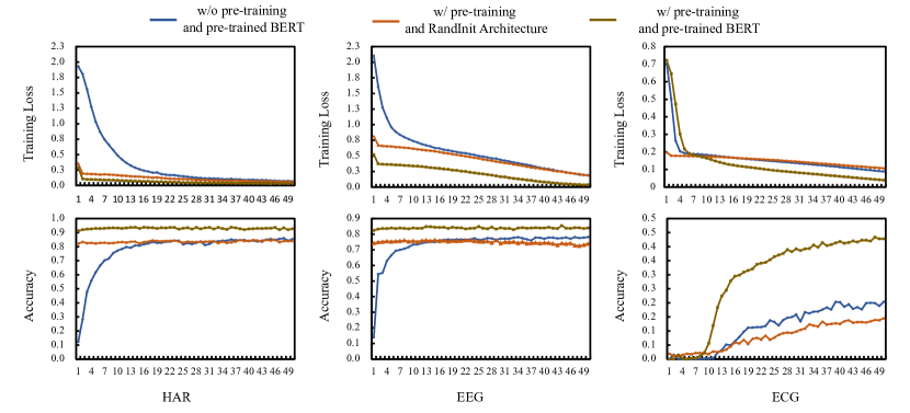
As shown in Figure 2, across all three datasets, the pre-trained BERT model consistently demonstrates superior convergence and accuracy. Training loss decreases more smoothly, and accuracy increases more rapidly compared to models without pre-training or with a BERT-like architecture. The consistent pattern across different data types underscores the effectiveness of pre-training in leveraging learned representations to achieve higher performance metrics, indicating a clear advantage of pre-trained models in processing sequential data.

Figure 3. Visualization of attention weight regarding to three different datasets.

5.2.8. Attention on Positions

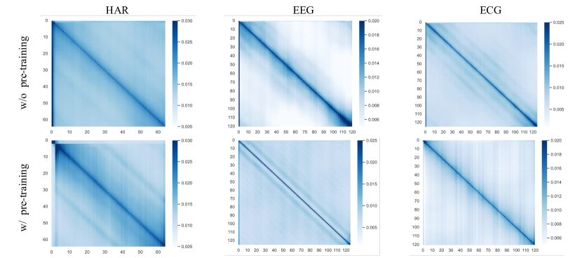
In the experimental analysis, we investigated the influence of pre-training on attention mechanisms across three distinct datasets: HAR, EEG, and ECG. Employing a comparative approach, we visualized attention weights using heatmaps to discern patterns indicative of the model’s focus. For each dataset, we analyzed two conditions: with and without pre-training. The HAR data revealed a pronounced diagonal pattern without pre-training, suggesting a strong self-attention to temporal features, which became more dispersed upon pre-training, indicating a more complex relational understanding. The EEG data presented a less distinct diagonal pattern, with pre-training enhancing temporal structure comprehension. Conversely, the ECG data displayed a consistent focus on temporal autocorrelation, with minimal variations observed between pre-trained and non-pre-trained models. These visualizations underscore the varying impact of pre-training on attention-based models, reflecting the inherent complexities of each dataset.

5.3. Limitation Analysis

Although its effectiveness of the CrossTimeNet, we also realize that there exist some inherent limitations within our work. This study presents an innovative self-supervised pre-training method across domains, empirically demonstrating knowledge transfer within the same tasks but not exploring transferability across diverse tasks (Cao et al., 2023). Despite showing promising results using PLM as the encoder, the research lacks a comprehensive theoretical explanation for its effectiveness. Additionally, our work have not investigated the potential of generative text models for a more universal modeling approach, which could align with the emerging trend of a single model addressing multiple language modeling tasks (Li et al., 2023; Ouyang et al., 2022).

6. Conclusion

In this study, we proposed CrossTimeNet, a novel self-supervised pre-training method designed for time series representation pre-training. Our method’s key feature is the time series data discretization, enabling cross-domain self-supervised pre-training. This approach empowers CrossTimeNet to harness temporal dynamics across diverse domains, leading to a versatile and transferable base model. Extensive experiments confirmed CrossTimeNet’s effectiveness in learning meaningful and transferable representations, providing substantial benefits for downstream tasks. We hope the CrossTimeNet will inspire more work to be proposed in the future.

Appendix

Appendix A Detail of Datasets

To evaluate the effectiveness of our proposed cross-domain self-supervised pre-training method, we selected three time series datasets from distinct domains, each representing a unique set of challenges and characteristics. These datasets facilitate a comprehensive assessment across varied scenarios, highlighting the adaptability and robustness of our approach.

• HAR: The Human Activity Recognition (HAR) dataset is a multi-class classification dataset that consists of sensor data collected from subjects performing various activities. The activities include walking, sitting, standing, and more complex activities like ascending or descending stairs. The data is captured using wearable sensors, providing a rich source of temporal patterns for recognizing human activities.

• EEG: The EEG datasets (a.k.a Sleep-EDF) comprises polysomnographic (PSG) recordings, which are used for multi-class sleep stage classification. The dataset includes Electroencephalogram (EEG) recordings among other physiological signals, collected from subjects under normal and pathological conditions. This dataset is pivotal for developing models that can automatically identify sleep stages, aiding in the diagnosis and study of sleep disorders.

• ECG: The China Physiological Signal Challenge (CPSC) dataset is a multi-label classification dataset containing Electrocardiogram (ECG) recordings. The dataset is designed for the detection of arrhythmias and other cardiac abnormalities. It provides a diverse set of ECG recordings, making it suitable for developing and evaluating models aimed at cardiac monitoring and diagnosis.

Table 7. Statics of used datasets in our experiments.

Dataset	#Train	#Test	Length	#Channel	#Class
HAR	8,823	2,947	128	9	6
EEG	12,787	1,421	3,000	2	8
ECG	10,854	1,206	5,000	12	27

Table 7 summarizes the key statistics and characteristics of these datasets, including the number of samples, channels, and classes. It is evident that there are significant differences among the datasets in terms of their dimensions and the diversity of classes they encompass. Note that both HAR and EEG data refer to multi-class classification task while ECG involve multi-label classification. It is also worth noting that for the construction of the pre-training dataset, these three datasets were mixed and shuffled together, preserving the train-test splits consistent with previous works in each domain. This approach ensures that our model is exposed to a diverse range of patterns and challenges, simulating real-world scenarios where domain shifts are common.

Appendix B Additional Implementation Details

B.1. Compared Baselines and Implement Details

To evaluate the efficacy of our cross-domain self-supervised pre-training approach, we compare it against several recent and popular self-supervised pre-training methods for time series data. These baseline methods encompass both reconstruction-based and contrastive learning approaches, ensuring a comprehensive comparison across different self-supervised learning paradigms.

• TST: A reconstruction-based self-supervised method that leverages a Transformer architecture to model time series data by predicting missing segments or forecasting future values. Despite its primary focus on reconstruction, we also consider a variant of TST without the self-supervised pre-training as a baseline to understand the impact of pre-training.

• TimeMAE : Similar to TST, TimeMAE employs a masked autoencoder framework for time series, where portions of the input data are masked out and the model learns to reconstruct the original data, enabling it to capture intrinsic temporal dynamics.

• TNC : A contrastive learning approach that treats close temporal segments as positive pairs and distant segments as negative pairs, encouraging the model to learn discriminative features by distinguishing between them.

• TS-TCC : This method extends the contrastive learning framework to time series data by leveraging temporal coherence as a signal for similarity, aiming to learn representations that are invariant to specific transformations while maintaining temporal structure.

• TS2Vec: A hierarchical contrastive learning approach that captures multi-scale temporal patterns by contrasting representations at different time scales, facilitating a comprehensive understanding of the time series data.

To ensure a fair comparison, all baseline methods employ an encoder network based on the Transformer architecture, maintaining consistency in the model’s capacity and structural complexity. During the fine-tuning phase for downstream tasks, the classification layer remains identical across all models, ensuring that any observed performance differences can be attributed to the effectiveness of the pre-training strategy rather than variations in the network architecture or task-specific adaptations. In terms of the hyper-parameter settings, the batch size is set to $32$, the remain ones are either strictly followed the specific settings suggested by the original paper or tuned the validation sets. We report the results of each baseline under its optimal hyper-parameter settings.

B.2. Specific Model Configurations of Our CrossTimeNet

Next, we delve into the intricate details of implementing the CrossTimeNet method, particularly focusing on the time series tokenization process using auto-encoder reconstruction architecture. For the tokenization component, the encoder network is meticulously designed with multiple layer TCN network to ensure efficient encoding of time series data into a compact representation. Specifically, the encoder network comprises four layers, facilitating a robust feature extraction mechanism. The embedding size is set to $64$. For the codebook number, we consistently set it as $512$ in all datasets. As for the patch size, we respectively set it as $2$, $25$, $40$ in the datasets of HAR, EEG, ECG. The network initialized is implemented with random manner. As for the optimization setting, learning rate is set as $5e^{-4}$ accompanied by the Adam optimizer. During the pre-training phase, we carefully tuned several hyperparameters to optimize the learning process. These include the learning rate, set to $1e^{-4}$, and the batch size chosen to be $32$. For the fine-tuning phase, we explored two distinct strategies: full fine-tuning and linear evaluation. All parameters of the pre-trained CrossTimeNet model are updated during training on the downstream tasks with preserving the same hyper-parameter settings as pre-training phase.

Appendix C Extended Analysis of Experimental Results

C.1. Results Across Varying Codebook Sizes

Next, we investigate the impact of varying the number of tokens in the codebook on the performance of CrossTimeNet. Table 8 show how downstream classification and reconstruction metrics of tokenization respond to changes in codebook size across three datasets. The findings reveal a general trend where increasing the codebook size up to a certain point leads to improvements in accuracy and F1 scores, particularly noticeable in the HAR dataset with the peak performance at a codebook size of $768$. However, larger codebook sizes also correlate with decreased coverage and increased MSE in some cases, indicating a potential overfitting or inefficiency in representation as the codebook size grows. In summary, the experiment highlights a trade-off between model expressiveness and its ability to generalize, suggesting an optimal codebook size range that maximizes performance while maintaining efficient data representation. This balance is crucial for the effective application of CrossTimeNet in processing sequential data across various domains.

Table 8. Performance comparison of our CrossTimeNet with different number of token in codebook.

Datasets	Size	Accuracy	F1 Score	Coverage	MSE
HAR	128	0.9298	0.931	1	0.0091
	256	0.9335	0.9348	1	0.0088
	384	0.9352	0.9366	1	0.0069
	512	0.9335	0.9347	0.7422	0.0082
	768	0.9389	0.9401	0.6237	0.0077
EEG	128	0.8656	0.6549	0.9922	0.0102
	256	0.8629	0.6335	0.4648	0.0103
	384	0.8635	0.6596	0.4453	0.0096
	512	0.8541	0.6402	0.2793	0.0099
	768	0.8543	0.8384	0.1849	0.0098
ECG	128	0.4187	0.5995	1	0.0055
	256	0.4146	0.6054	1	0.0051
	384	0.4179	0.5953	1	0.0047
	512	0.4378	0.6278	0.5918	0.0047
	768	0.4328	0.6118	0.4714	0.0048

C.2. Results Across Varying Patch Sizes

Table 9 presents a comprehensive evaluation of our CrossTimeNet model’s performance with varying patch sizes. Notably, a patch size of $40$ achieves the optimal model performance. However, this configuration exhibits a reduced coverage of 0.5918, suggesting a trade-off between model precision and its ability to generalize across the entire data set. On the other hand, the smallest patch size (20) ensures complete Coverage but with slightly lower accuracy and F1 scores, alongside the lowest MSE (0.0033), implying better model predictions. As the patch size increases beyond 40, there is a noticeable decline in all performance metrics, with Accuracy and F1 Score decreasing, and MSE progressively increasing, indicating diminishing returns in model performance. This trend underscores the critical impact of patch size on the efficacy of the CrossTimeNet model, highlighting the necessity to balance between model granularity and computational efficiency for optimal performance.

Table 9. Performance comparison of our CrossTimeNet with different patch sizes.

Patch Size	Accuracy	F1 Score	Coverage	MSE
20	0.4063	0.6051	1.0000	0.0033
40	0.4287	0.6161	0.5918	0.0047
60	0.4163	0.5935	0.4609	0.0057
80	0.3856	0.5627	0.4629	0.0066
100	0.3822	0.5295	0.2891	0.0078

Table 10. CrossTimeNet performance with varied random word mappings across three repetitions, denoted by A, B, C.

Evaluation Manners	Models	HAR		EEG		ECG
		Accuracy	F1 Score	Accuracy	F1 Score	Accuracy	F1 Score
Full Fine-tuning	A	0.9325	0.9339	0.8529	0.6401	0.4395	0.6293
	B	0.9345	0.9357	0.8543	0.6403	0.4336	0.6218
	C	0.9335	0.9345	0.8550	0.6402	0.4403	0.6324
Linear Evaluation	A	0.9155	0.9152	0.8388	0.5923	0.2180	0.3259
	B	0.9182	0.9189	0.8276	0.5827	0.2231	0.3323
	C	0.9223	0.9232	0.8332	0.6050	0.2255	0.3358

Table 11. Exploring pre-training dataset construction for CrossTimeNet: sequential vs. mixing ordering across domains.

Fine-tuning Strategies	Data Mixing Strategy	HAR		EEG		ECG
		Accuracy	F1 Score	Accuracy	F1 Score	Accuracy	F1 Score
Full Fine-tuning	HAR-ECG-EEG	0.8999	0.8992	0.8487	0.6324	0.3689	0.5393
	ECG-EEG-HAR	0.9315	0.9325	0.8388	0.6064	0.3275	0.5021
	HAR-EEG-ECG	0.8646	0.8620	0.8290	0.5972	0.4245	0.6166
	Domain-agnostic Mixing	0.9335	0.9347	0.8541	0.6402	0.4378	0.6278
Linear Evaluation	HAR-ECG-EEG	0.7910	0.7857	0.8367	0.6137	0.1310	0.2005
	ECG-EEG-HAR	0.9182	0.9184	0.8044	0.5619	0.1144	0.1723
	HAR-EEG-ECG	0.7777	0.7714	0.7650	0.5017	0.2114	0.3153
	Domain-agnostic Mixing	0.9146	0.9148	0.8381	0.6072	0.2134	0.3148

Figure 4. Investigating the impact of downstream training set sparsity on fine-tuning pre-trained model.

Figure 5. T-SNE visualization of sequence of patches in a instance and its corresponding raw time series.

C.3. Studying the Token Selection Strategies

Table 10 presents the performance of CrossTimeNet under different random word mappings (denoted as A, B, and C) across three distinct datasets. Observing the results, it is evident that the variations in word mappings have a relatively minor influence on the overall performance metrics. This result underlines the effectiveness of the word mapping mechanism in bridging the representational gap between time series tokens and the BERT model’s vocabulary, thereby enabling the CrossTimeNet to leverage pre-trained language model representations for time series analysis tasks.

C.4. Impact of Pre-training Dataset Construction

In this part, our goal is to explore how the arrangement of pre-training data from different domains affects the model’s effectiveness. Specifically, sequential domain-specific ordering to domain-agnostic mixing are employed as model variants. Table 11 presents the performance metrics under different data mixing strategies and fine-tuning approaches. Overall, the results indicate that domain-agnostic mixing, where pre-training data from various domains is intermixed without a specific sequence, leads to superior performance across all metrics and datasets compared to sequential domain-specific arrangements. This is evident in both full fine-tuning and Linear Evaluation strategies, where domain-agnostic mixing consistently achieves the highest accuracy and F1 scores. For instance, in the full fine-tuning strategy, domain-agnostic mixing outperforms the sequential arrangements with notable margins in both HAR and ECG datasets. These findings suggest that a domain-agnostic approach to pre-training data mixing enhances the model’s ability to generalize across different domains, likely due to a more diverse and comprehensive representation of features. This approach appears to mitigate overfitting to domain-specific characteristics, leading to improved overall performance.

C.5. Data Sparsity Analysis

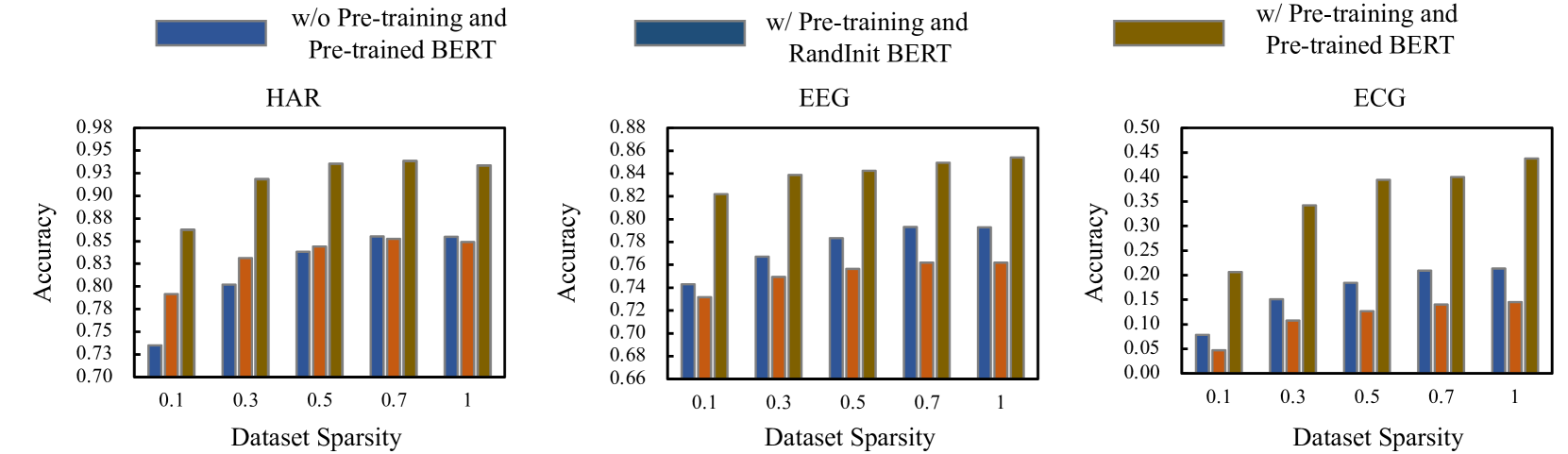
Figure 4 illustrates the accuracy of fine-tuning a pre-trained model across varying degrees of training set sparsity in three datasets. Overall, the accuracy of the fine-tuned pre-trained model exhibits a general decline as dataset sparsity increases. This indicates that denser datasets tend to yield better fine-tuning outcomes, affirming the importance of data richness for model performance optimization. Despite the overall trend, the pre-trained BERT model demonstrates a notable degree of robustness to sparsity, maintaining higher accuracy relative to the model without pre-training and the RandomInit BERT. This robustness is especially evident in the ECG domain, where accuracy remains relatively stable until a sparsity level of $0.5$, suggesting that pre-trained models can leverage their learned representations to effectively handle sparse data. In summary, while dataset sparsity negatively impacts model accuracy, pre-training can serve as a mitigating factor, enhancing the model’s ability to maintain performance in sparse data conditions. This underscores the potential of pre-trained models in applications with data limitations.

C.6. Analyzing Semantic of Time Series Token

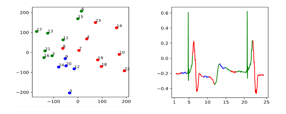
The case study employs t-SNE visualization to articulate the clustering of discrete tokens represented in a high-dimensional feature space, juxtaposed with their manifestation in the corresponding raw time series data. The t-SNE plot distinctly segregates the tokens into coherent clusters, demarcated by a trio of colors, each color signifying a unique token category. This delineation by the t-SNE algorithm evidences its capability to reduce dimensionality while preserving the topology of the dataset, facilitating an intuitive understanding of complex structures within the feature space.

Parallelly, the time series graph delineates these tokens across the temporal axis, with the color-coded segments reflecting the same categorical distinctions identified in the t-SNE visualization. The synchronization between the spatial clusters in the t-SNE plot and the temporal segmentation in the time series data provides a compelling narrative of the data’s underlying dynamics. Each color-coded point, representing a discrete token, aligns with a specific behavior or state in the time series, thereby mapping a multi-dimensional data narrative onto a comprehensible two-dimensional framework.

This analytical approach, combining t-SNE with time series visualization, serves as an effective method for interpreting the nuanced interactions of tokens over time, offering a profound lens through which data scientists can observe temporal patterns, detect anomalies, or even predict future states in sequential data models.

References

- (1)
- Cao et al. (2023) Defu Cao, Furong Jia, Sercan O Arik, Tomas Pfister, Yixiang Zheng, Wen Ye, and Yan Liu. 2023. Tempo: Prompt-based generative pre-trained transformer for time series forecasting. arXiv preprint arXiv:2310.04948 (2023).
- Cheng et al. (2023a) Mingyue Cheng, Qi Liu, Zhiding Liu, Zhi Li, Yucong Luo, and Enhong Chen. 2023a. FormerTime: Hierarchical Multi-Scale Representations for Multivariate Time Series Classification. arXiv preprint arXiv:2302.09818 (2023).
- Cheng et al. (2023b) Mingyue Cheng, Qi Liu, Zhiding Liu, Hao Zhang, Rujiao Zhang, and Enhong Chen. 2023b. TimeMAE: Self-Supervised Representations of Time Series with Decoupled Masked Autoencoders. arXiv preprint arXiv:2303.00320 (2023).
- Cheng et al. (2024) Mingyue Cheng, Jiqian Yang, Tingyue Pan, Qi Liu, and Zhi Li. 2024. ConvTimeNet: A Deep Hierarchical Fully Convolutional Model for Multivariate Time Series Analysis. arXiv preprint arXiv:2403.01493 (2024).
- Christ et al. (2018) Maximilian Christ, Nils Braun, Julius Neuffer, and Andreas W Kempa-Liehr. 2018. Time series feature extraction on basis of scalable hypothesis tests (tsfresh–a python package). Neurocomputing 307 (2018), 72–77.
- Dehaene-Lambertz (2017) Ghislaine Dehaene-Lambertz. 2017. The human infant brain: A neural architecture able to learn language. Psychonomic bulletin & review 24 (2017), 48–55.
- Deng et al. (2013) Houtao Deng, George Runger, Eugene Tuv, and Martyanov Vladimir. 2013. A time series forest for classification and feature extraction. Information Sciences 239 (2013), 142–153.
- Devlin et al. (2018) Jacob Devlin, Ming-Wei Chang, Kenton Lee, and Kristina Toutanova. 2018. Bert: Pre-training of deep bidirectional transformers for language understanding. arXiv preprint arXiv:1810.04805 (2018).
- Ding et al. (2008) Hui Ding, Goce Trajcevski, Peter Scheuermann, Xiaoyue Wang, and Eamonn Keogh. 2008. Querying and mining of time series data: experimental comparison of representations and distance measures. Proceedings of the VLDB Endowment 1, 2 (2008), 1542–1552.
- Eldele et al. (2021) Emadeldeen Eldele, Mohamed Ragab, Zhenghua Chen, Min Wu, Chee Keong Kwoh, Xiaoli Li, and Cuntai Guan. 2021. Time-series representation learning via temporal and contextual contrasting. arXiv preprint arXiv:2106.14112 (2021).
- Fedus et al. (2022) William Fedus, Barret Zoph, and Noam Shazeer. 2022. Switch transformers: Scaling to trillion parameter models with simple and efficient sparsity. The Journal of Machine Learning Research 23, 1 (2022), 5232–5270.
- Fu et al. (2023) Junchen Fu, Fajie Yuan, Yu Song, Zheng Yuan, Mingyue Cheng, Shenghui Cheng, Jiaqi Zhang, Jie Wang, and Yunzhu Pan. 2023. Exploring Adapter-based Transfer Learning for Recommender Systems: Empirical Studies and Practical Insights. arXiv preprint arXiv:2305.15036 (2023).
- Grabocka et al. (2014) Josif Grabocka, Nicolas Schilling, Martin Wistuba, and Lars Schmidt-Thieme. 2014. Learning time-series shapelets. In Proceedings of the 20th ACM SIGKDD international conference on Knowledge discovery and data mining. 392–401.
- Han et al. (2023) Lu Han, Han-Jia Ye, and De-Chuan Zhan. 2023. The Capacity and Robustness Trade-off: Revisiting the Channel Independent Strategy for Multivariate Time Series Forecasting. arXiv preprint arXiv:2304.05206 (2023).
- He et al. (2022) Kaiming He, Xinlei Chen, Saining Xie, Yanghao Li, Piotr Dollár, and Ross Girshick. 2022. Masked autoencoders are scalable vision learners. In Proceedings of the IEEE/CVF conference on computer vision and pattern recognition. 16000–16009.
- Hu et al. (2021) Edward J Hu, Yelong Shen, Phillip Wallis, Zeyuan Allen-Zhu, Yuanzhi Li, Shean Wang, Lu Wang, and Weizhu Chen. 2021. Lora: Low-rank adaptation of large language models. arXiv preprint arXiv:2106.09685 (2021).
- Ismail Fawaz et al. (2019) Hassan Ismail Fawaz, Germain Forestier, Jonathan Weber, Lhassane Idoumghar, and Pierre-Alain Muller. 2019. Deep learning for time series classification: a review. Data mining and knowledge discovery 33, 4 (2019), 917–963.
- Kao and Lee (2021) Wei-Tsung Kao and Hung-yi Lee. 2021. Is BERT a Cross-Disciplinary Knowledge Learner? A Surprising Finding of Pre-trained Models’ Transferability. arXiv preprint arXiv:2103.07162 (2021).
- Kenton and Toutanova (2019) Jacob Devlin Ming-Wei Chang Kenton and Lee Kristina Toutanova. 2019. BERT: Pre-training of Deep Bidirectional Transformers for Language Understanding. In Proceedings of NAACL-HLT. 4171–4186.
- Kong and Zhang (2023) Xiangwen Kong and Xiangyu Zhang. 2023. Understanding masked image modeling via learning occlusion invariant feature. In Proceedings of the IEEE/CVF Conference on Computer Vision and Pattern Recognition. 6241–6251.
- Kostelich and Schreiber (1993) Eric J Kostelich and Thomas Schreiber. 1993. Noise reduction in chaotic time-series data: A survey of common methods. Physical Review E 48, 3 (1993), 1752.
- Li et al. (2023) Jun Li, Che Liu, Sibo Cheng, Rossella Arcucci, and Shenda Hong. 2023. Frozen Language Model Helps ECG Zero-Shot Learning. arXiv preprint arXiv:2303.12311 (2023).
- Lin et al. (2007) Jessica Lin, Eamonn Keogh, Li Wei, and Stefano Lonardi. 2007. Experiencing SAX: a novel symbolic representation of time series. Data Mining and knowledge discovery 15 (2007), 107–144.
- Lin et al. (2012) Jessica Lin, Rohan Khade, and Yuan Li. 2012. Rotation-invariant similarity in time series using bag-of-patterns representation. Journal of Intelligent Information Systems 39 (2012), 287–315.
- Liu et al. (2021) Minghao Liu, Shengqi Ren, Siyuan Ma, Jiahui Jiao, Yizhou Chen, Zhiguang Wang, and Wei Song. 2021. Gated transformer networks for multivariate time series classification. arXiv preprint arXiv:2103.14438 (2021).
- Liu et al. (2019) Yinhan Liu, Myle Ott, Naman Goyal, Jingfei Du, Mandar Joshi, Danqi Chen, Omer Levy, Mike Lewis, Luke Zettlemoyer, and Veselin Stoyanov. 2019. Roberta: A robustly optimized bert pretraining approach. arXiv preprint arXiv:1907.11692 (2019).
- Liu et al. (2024a) Zhiding Liu, Mingyue Cheng, Zhi Li, Zhenya Huang, Qi Liu, Yanhu Xie, and Enhong Chen. 2024a. Adaptive normalization for non-stationary time series forecasting: A temporal slice perspective. Advances in Neural Information Processing Systems 36 (2024).
- Liu et al. (2024b) Zhiding Liu, Jiqian Yang, Mingyue Cheng, Yucong Luo, and Zhi Li. 2024b. Generative Pretrained Hierarchical Transformer for Time Series Forecasting. arXiv preprint arXiv:2402.16516 (2024).
- Middlehurst et al. (2023) Matthew Middlehurst, Patrick Schäfer, and Anthony Bagnall. 2023. Bake off redux: a review and experimental evaluation of recent time series classification algorithms. arXiv preprint arXiv:2304.13029 (2023).
- Oord et al. (2016) Aaron van den Oord, Sander Dieleman, Heiga Zen, Karen Simonyan, Oriol Vinyals, Alex Graves, Nal Kalchbrenner, Andrew Senior, and Koray Kavukcuoglu. 2016. Wavenet: A generative model for raw audio. arXiv preprint arXiv:1609.03499 (2016).
- Oord et al. (2018) Aaron van den Oord, Yazhe Li, and Oriol Vinyals. 2018. Representation learning with contrastive predictive coding. arXiv preprint arXiv:1807.03748 (2018).
- Ouyang et al. (2022) Long Ouyang, Jeffrey Wu, Xu Jiang, Diogo Almeida, Carroll Wainwright, Pamela Mishkin, Chong Zhang, Sandhini Agarwal, Katarina Slama, Alex Ray, et al. 2022. Training language models to follow instructions with human feedback. Advances in Neural Information Processing Systems 35 (2022), 27730–27744.
- Radford et al. (2019) Alec Radford, Jeffrey Wu, Rewon Child, David Luan, Dario Amodei, Ilya Sutskever, et al. 2019. Language models are unsupervised multitask learners. OpenAI blog 1, 8 (2019), 9.
- Schäfer (2015) Patrick Schäfer. 2015. The BOSS is concerned with time series classification in the presence of noise. Data Mining and Knowledge Discovery 29 (2015), 1505–1530.
- Schäfer and Högqvist (2012) Patrick Schäfer and Mikael Högqvist. 2012. SFA: a symbolic fourier approximation and index for similarity search in high dimensional datasets. In Proceedings of the 15th international conference on extending database technology. 516–527.
- Senin and Malinchik (2013) Pavel Senin and Sergey Malinchik. 2013. Sax-vsm: Interpretable time series classification using sax and vector space model. In 2013 IEEE 13th international conference on data mining. IEEE, 1175–1180.
- Shifaz et al. (2020) Ahmed Shifaz, Charlotte Pelletier, François Petitjean, and Geoffrey I Webb. 2020. TS-CHIEF: a scalable and accurate forest algorithm for time series classification. Data Mining and Knowledge Discovery 34, 3 (2020), 742–775.
- Tonekaboni et al. (2021) Sana Tonekaboni, Danny Eytan, and Anna Goldenberg. 2021. Unsupervised representation learning for time series with temporal neighborhood coding. arXiv preprint arXiv:2106.00750 (2021).
- Van Den Oord et al. (2017) Aaron Van Den Oord, Oriol Vinyals, et al. 2017. Neural discrete representation learning. Advances in neural information processing systems 30 (2017).
- Vaswani et al. (2017) Ashish Vaswani, Noam Shazeer, Niki Parmar, Jakob Uszkoreit, Llion Jones, Aidan N Gomez, Łukasz Kaiser, and Illia Polosukhin. 2017. Attention is all you need. Advances in neural information processing systems 30 (2017).
- Wang et al. (2017) Zhiguang Wang, Weizhong Yan, and Tim Oates. 2017. Time series classification from scratch with deep neural networks: A strong baseline. In 2017 International joint conference on neural networks (IJCNN). IEEE, 1578–1585.
- Wen et al. (2022) Qingsong Wen, Tian Zhou, Chaoli Zhang, Weiqi Chen, Ziqing Ma, Junchi Yan, and Liang Sun. 2022. Transformers in time series: A survey. arXiv preprint arXiv:2202.07125 (2022).
- Yang et al. (2021) Chao-Han Huck Yang, Yun-Yun Tsai, and Pin-Yu Chen. 2021. Voice2series: Reprogramming acoustic models for time series classification. In International conference on machine learning. PMLR, 11808–11819.
- Ye and Keogh (2009) Lexiang Ye and Eamonn Keogh. 2009. Time series shapelets: a new primitive for data mining. In Proceedings of the 15th ACM SIGKDD international conference on Knowledge discovery and data mining. 947–956.
- Yue et al. (2022) Zhihan Yue, Yujing Wang, Juanyong Duan, Tianmeng Yang, Congrui Huang, Yunhai Tong, and Bixiong Xu. 2022. Ts2vec: Towards universal representation of time series. In Proceedings of the AAAI Conference on Artificial Intelligence, Vol. 36. 8980–8987.
- Zerveas et al. (2021) George Zerveas, Srideepika Jayaraman, Dhaval Patel, Anuradha Bhamidipaty, and Carsten Eickhoff. 2021. A transformer-based framework for multivariate time series representation learning. In Proceedings of the 27th ACM SIGKDD conference on knowledge discovery & data mining. 2114–2124.
- Zhang et al. (2023) Kexin Zhang, Qingsong Wen, Chaoli Zhang, Rongyao Cai, Ming Jin, Yong Liu, James Zhang, Yuxuan Liang, Guansong Pang, Dongjin Song, et al. 2023. Self-Supervised Learning for Time Series Analysis: Taxonomy, Progress, and Prospects. arXiv preprint arXiv:2306.10125 (2023).
- Zhang et al. (2020) Xuchao Zhang, Yifeng Gao, Jessica Lin, and Chang-Tien Lu. 2020. Tapnet: Multivariate time series classification with attentional prototypical network. In Proceedings of the AAAI Conference on Artificial Intelligence, Vol. 34. 6845–6852.
- Zheng et al. (2014) Yi Zheng, Qi Liu, Enhong Chen, Yong Ge, and J Leon Zhao. 2014. Time series classification using multi-channels deep convolutional neural networks. In International conference on web-age information management. Springer, 298–310.