Scaling Value Iteration Networks to 5000 Layers
for Extreme Long-Term Planning

Abstract

The Value Iteration Network (VIN) is an end-to-end differentiable architecture that performs value iteration on a latent MDP for planning in reinforcement learning (RL). However, VINs struggle to scale to long-term and large-scale planning tasks, such as navigating a $100\times 100$ maze—a task which typically requires thousands of planning steps to solve. We observe that this deficiency is due to two issues: the representation capacity of the latent MDP and the planning module’s depth. We address these by augmenting the latent MDP with a dynamic transition kernel, dramatically improving its representational capacity, and, to mitigate the vanishing gradient problem, introduce an “adaptive highway loss” that constructs skip connections to improve gradient flow. We evaluate our method on both 2D maze navigation environments and the ViZDoom 3D navigation benchmark. We find that our new method, named Dynamic Transition VIN (DT-VIN), easily scales to 5000 layers and casually solves challenging versions of the above tasks. Altogether, we believe that DT-VIN represents a concrete step forward in performing long-term large-scale planning in RL environments.

1 Introduction

Planning is the problem of finding a sequence of actions that achieve a specific pre-defined goal. As the aim of both some older algorithms (e.g., Dyna sutton1991dyna, A* hart1968formal, and others Schmidhuber:90diffgenau,Schmidhuber:90sandiego) and many recent ones (e.g., the Predictron silver2017predictron, the Dreamer family of algorithms hafner2020dream,hafner2021mastering,hafner2023mastering, SoRB eysenbach2019search, SA-CADRL chen2017socially, and the LLM-planner song2023llm), effective planning is a long-standing and important challenge in artificial intelligence (AI). Within reinforcement learning (RL), one particularly notable method is the Value Iteration Network (VIN) proposed by tamar2016value.

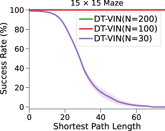
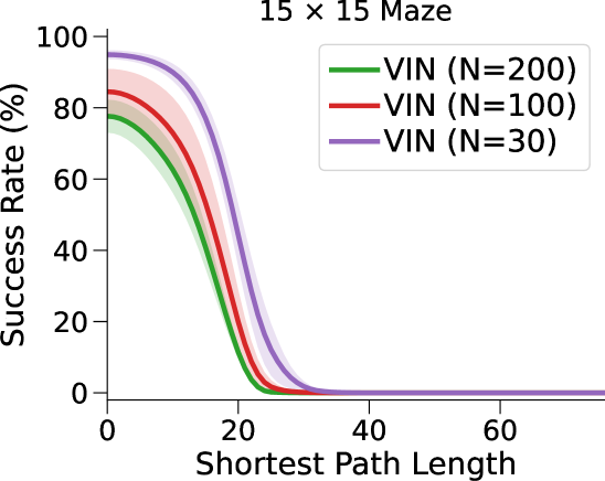
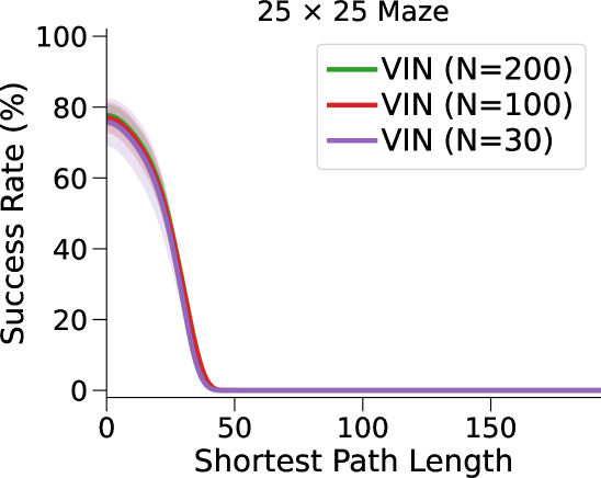
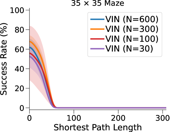
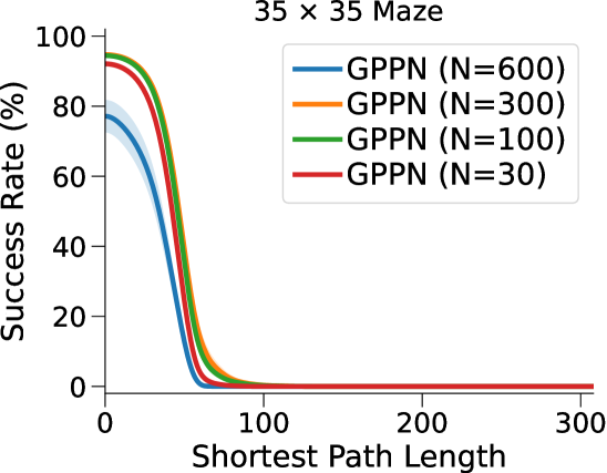
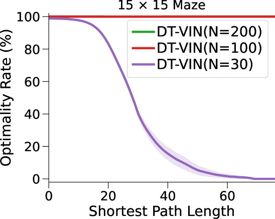
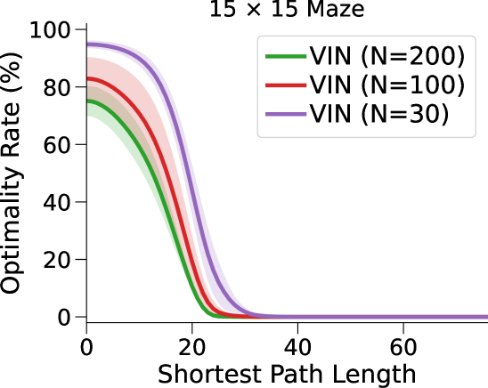
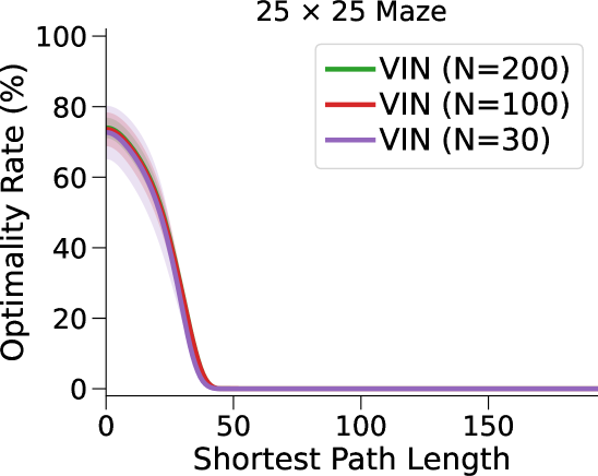
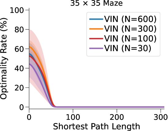
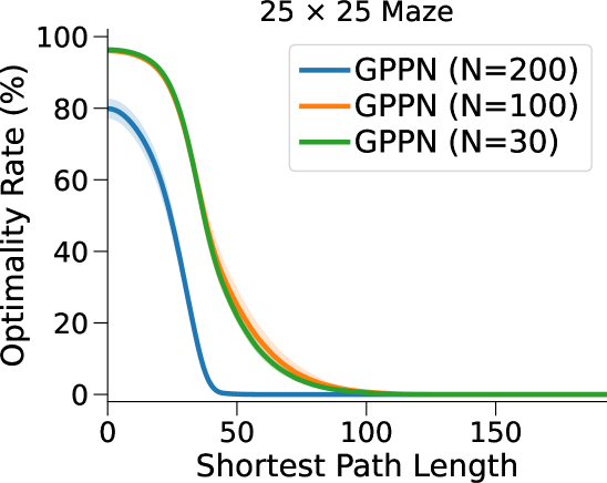
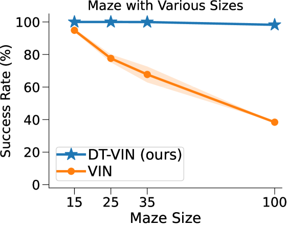
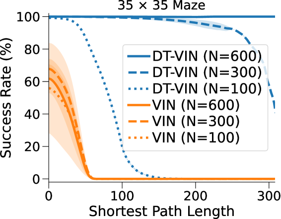
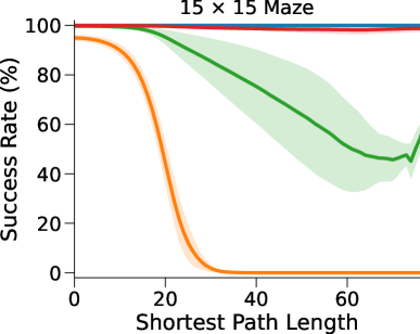
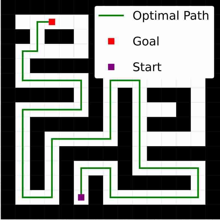
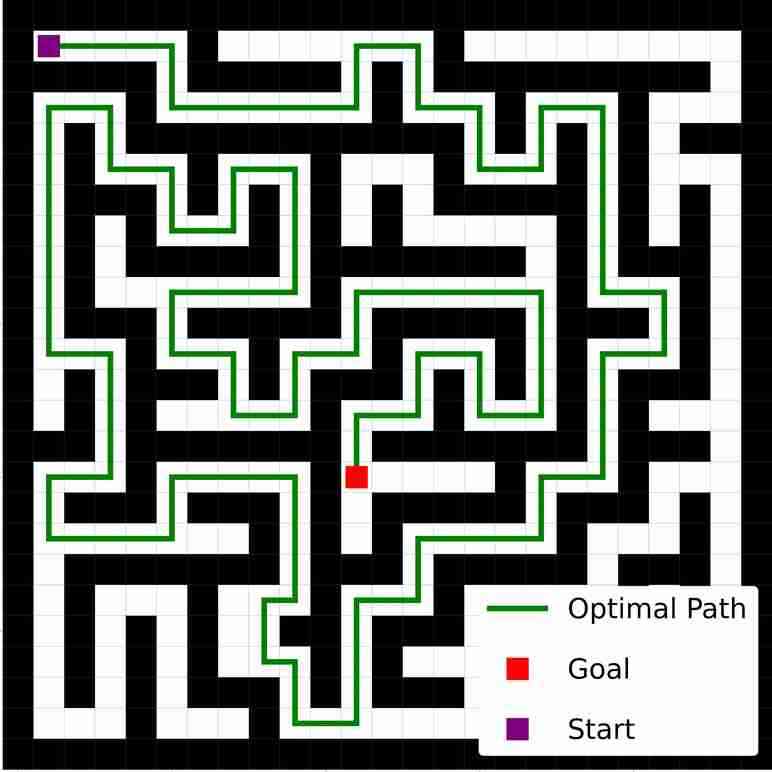
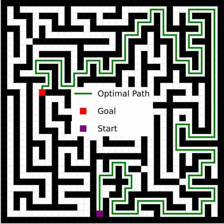
VIN is an artificial neural network (NN) architecture designed for planning, incorporating a differentiable “planning module” that performs value iteration bellman1966dynamic on a “latent MDP.” VINs have been shown to perform exceptionally well in some small-scale short-term planning situations, like path planning pflueger2019rover,jin2021value, autonomous navigation wohlke2021hierarchies, and complex decision-making in dynamic environments li2021dynamic. However, they still struggle to solve larger-scale and longer-term planning problems. For example, in a $100\times 100$ maze navigation task, the success rate of VINs in reaching the goal drops to well below 40% (see Figure 1(b)). Even in smaller $35\times 35$ mazes, the success rate of VINs drop to 0% when the required planning steps exceed 60 (see Figure 1(c)).

Our work identifies that the principal deficiency causing this is the mismatch between the complexity of planning and the comparatively weak representational capacity of the relatively shallow networks that it uses. And while there has been moderate success in learning more complicated networks (e.g., GPPN lee2018gated and Highway VINs wang2024highway), until now, VINs of a scale capable of long-term or large-scale planning have not been computationally tractable due to persistent issues with vanishing and exploding gradients—a fundamental problem of deep learning Hochreiter:91.

In this work, we aim to surgically correct deficiencies in VIN-based architectures to enable large-scale long-term planning. Specifically, we first identify the limitations of the latent MDP in VIN and propose a dynamic transition kernel to dramatically increase the representational capacity of the network. We then build on existing work that identifies the connection between network depth and long-term planning wang2024highway and propose an “adaptive highway loss” that selectively constructs skip connections to the final loss according to the actual number of planning steps. This approach helps mitigate the vanishing gradient problem and enables the training of very deep networks. With these changes, we find that our new Dynamic Transition Value Iteration Network (DT-VIN), is able to be trained with $5000$ layers and easily scale to $1800$ planning steps in a $100\times 100$ maze navigation task (compared to the original VIN, which only scaled to 120 planning steps in a $25\times 25$ maze). We apply our method to top-down image-based maze navigation tasks and the first-person image-based ViZDoom benchmark Wydmuch2019ViZDoom. We find that DT-VINs can easily solve both despite these problems requiring hundreds to thousands of planning steps. Together, these demonstrate the practical utility of our method on vision-based tasks that previous methods are simply unable to solve. This also serves to highlight the potential of our method to scale to increasingly complex planning tasks alongside the increasing availability of computing power.

(a)

(b)

(c)

Figure 1: 1(a) shows an example of $100\times 100$ maze navigation task, where the green line shows the optimal path from the start position (blue) to the goal position (red). See Figure 6 in Appendix B for more examples of mazes with other sizes. 1(b) shows the success rate of VIN and DT-VIN on the maze navigation tasks as a function of the size of the maze. The reported results are computed in expectation over different shortest path lengths for each maze size. 1(c) shows the success rate of VIN tamar2016value and DT-VIN for different network depths on the $35\times 35$ maze benchmark.

2 Preliminaries

Reinforcement Learning (RL).

The most common formalism used for RL is that of the Markov Decision Process (MDP) bellman1957markovian. We consider an MDP—as per puterman2014markov—to be the $6$-tuple ($𝒮,𝒜,𝒯,ℛ,\gamma ,\mu$), where $𝒮$ is a countable state space, $𝒜$ is a finite action space, $𝒯(s^{\prime }|s,a)$ represents the probability of transitioning to state $s^{\prime }\in 𝒮$ when being in state $s\in 𝒮$ and taking action $a\in 𝒜$, $ℛ(s,a,s^{\prime })$ is the scalar reward function, $\gamma \in [0,1)$ is a discount factor, and $\mu$ is a distribution over initial states. The behaviour of an artificial agent in an MDP is defined by its policy $\pi (a|s)$, which specifies the probability of taking action $a$ in state $s$. The state value function $V^{\pi }(s)$ is the expected discounted sum of rewards from state $s$ and following policy $\pi$, i.e., $V^{\pi }(s)\triangleq 𝔼\left[{\sum }_{t=0}^{\mathrm{\infty }}{\gamma }^tℛ(s_t,a_t,s_{t+1})|s_0=s;\pi \right]$. The goal of RL is usually to find an optimal policy ${\pi }^{\ast }$ that achieves the highest expected discounted sum of rewards. The value function of an optimal policy is denoted by $V^{\ast }(s)={\max }_{\pi }{V}^{\pi }(s)$, and satisfies $V^{{\pi }^{\ast }}(s)=V^{\ast }(s)\forall s$. The Value Iteration (VI) algorithm iteratively applies the following update to all states to obtain the optimal value function: $V^{(n+1)}(s)={\max }_a{\sum }_{s^{\prime }}𝒯\left(s^{\prime }|s,a\right)\left[ℛ(s,a,s^{\prime })+\gamma V^{(n)}\left(s^{\prime }\right)\right]$, where $n$ is the iteration number.

Convolutional Neural Networks (CNNs).

CNNs are neural networks that specialize in processing data with a grid structure, such as images Fukushima:1979neocognitron, waibel1987phoneme, zhang1988shift. A CNN forward pass typically involves several convolutional layers, where a learnable filter is used to slide across the input data and create a feature map, and max-pooling layers, where the dimension of the feature map is reduced. Formally, a stacked max-pooling and convolutional layer performs the following operation: $X_{c^{\prime },i,j}={\max }_{i^{\prime },j^{\prime }\in N(i,j)}\sigma \left({\sum }_{c,i,j}{W}_{c,i,j}^{c^{\prime }}{X}_{c,i^{\prime }-i,j^{\prime }-j}\right)$, where $\sigma$ is an activation function, $X$ is an image comprising $c$ channels, $W^1,\mathrm{\dots },W^{c^{\prime }}\in {ℝ}^{c\times F\times F}$ are kernels, and $N(i,j)$ denotes a $F\times F$ patch centered around pixel $(i,j)$.

Value Iteration Networks (VINs).

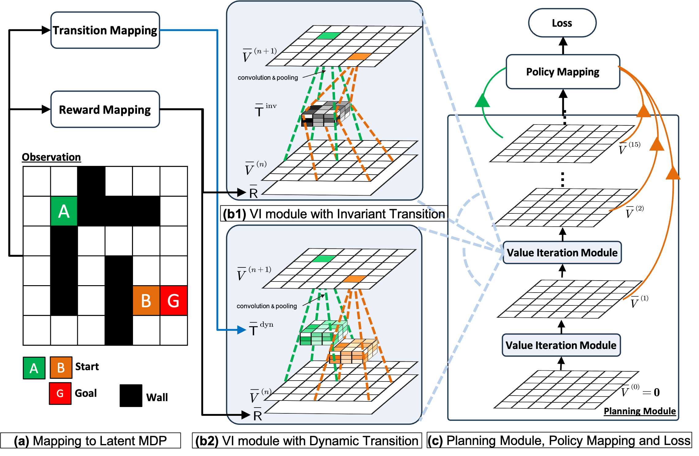
VIN is an end-to-end differentiable neural network architecture for planning which demonstrates strong generalization to unseen domains through the incorporation of an explicit planning module tamar2016value. The main idea of VIN is to map observations into a latent MDP $\overline{ℳ}$ and then use the embedded planning module to perform value iteration (VI) on this latent MDP. Below, we use $\overline{\cdot }$ to denote all the terms associated with the latent MDP $\overline{ℳ}$.

For each decision, VIN first maps an observation $x=\varphi (s)$, e.g., an image of a maze and the current position of the agent, to $\overline{ℳ}$. $\overline{ℳ}$ is described by the latent state space $\overline{𝒮}={\{(i,j)\}}_{i,j\in [m]}$; a fixed discrete latent action space $\overline{𝒜}$; a latent reward matrix $\overline{𝖱}=f^{\overline{𝖱}}(\varphi (s))\in {ℝ}^{m\times m}$, where $f^{\overline{𝖱}}$ is a learnable NN called a reward mapping module; and a latent transition matrix (or kernel) ${\overline{𝖳}}^{\mathrm{inv}}\in {ℝ}^{|\overline{𝒜}|\times F\times F}$. The latent transition matrix is a parameter matrix that is invariant for each latent state $(i,j)$, independent of the observation $x$, and not restricted to satisfy the probabilistic property, i.e., its elements are not required to represent probabilities or sum to one. Next, VIN conducts VI on the latent MDP $\overline{ℳ}$ to approximate the latent optimal value function ${\overline{V}}^{\ast }$. To ensure the differentiability of the VI computation, a differentiable VI module is proposed. This module simulates VI computation using differentiable CNN operations, i.e., convolutional and max-pooling operations: $$V¯i,j(n+1)=maxa¯⁢∑i′,j′𝖳¯a¯,i′,j′inv⁢(𝖱¯i−i′,j−j′+V¯i−i′,j−j′(n)), ⁢i,j∈[m]. This equation sums over a matrix patch centered around position $(i,j)$.

After the above, by stacking the VI module for $N$ layers, the latent value function is then fed to a policy mapping module by $f^{\pi }$ to represent a policy that is applicable to the actual MDP $ℳ$. Finally, the model can be trained by standard RL and IL algorithms with the following general loss: $ℒ\left(\theta \right)=\frac{1}{|𝒟|}{\sum }_{(x,y)\in 𝒟}\mathrm{\ell }(f^{\pi }\left({\overline{V}}^{(N)}(x)\right),y)$, where $𝒟=\{(x,y)\}$ is the training data, $x$ is the observation, $y$ is the label, and $\mathrm{\ell }$ is the sample-wise loss function. The specific meaning of these items varies depending on the task, e.g., in imitation learning, the label $y$ is the optimal action and $\mathrm{\ell }$ is the cross-entropy loss.

3 Method

In this section, we discuss how to train scalable VINs for long-term large-scale planning tasks. Our method addresses the two key issues with VIN that are identified as hampering its scalability: the capacity of the latent MDP representation and the depth of the planning module.

Figure 2: The architecture of VIN and DT-VIN in the maze navigation task. (a) shows the observation of the maze, which is mapped to the latent reward/transition matrix of the latent MDP through the reward/transition mapping module. (c) shows the “planning module”, the policy mapping module and the loss. The “planning module” contains numerous stacked Value Iteration (VI) modules. The green and orange connections show an example of adaptive highway loss for planning tasks starting from A and B, respectively. (b1) shows the VI module of the original VIN with invariant transition ${\overline{𝖳}}^{\mathrm{inv}}\in {ℝ}^{|𝒜|\times F\times F}$. (b2) shows the VI module of DT-VIN with dynamic transition kernel ${\overline{𝖳}}^{\mathrm{dyn}}\in {ℝ}^{m\times m\times |𝒜|\times F\times F}$.

3.1 Increasing the Representation Capacity of the Latent MDP

Motivation.

VIN utilizes the computational similarities between VI and CNNs to directly implement VI through a CNN-based VI module, as described in Section 2. However, there is a discrepancy between the CNN-based VI module and the general VI computation process.

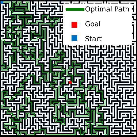
CNN-based VIN uses an invariant latent transition kernel ${\overline{𝖳}}^{\mathrm{inv}}\in {ℝ}^{|\overline{𝒜}|\times F\times F}$ as a learnable parameter, which is the same for each latent state $\overline{s}=(i,j)$ and independent of the current observation, e.g., the map of the maze. This severely limits the representational capacity of the latent MDP which, to be effective, should model what will in practice be the complex and state-dependent transition function of the actual MDP. For example, in the maze navigation problem shown in Figure 1(a), the transition probabilities are quite different if the adjacent cell is a wall versus an empty cell. Additionally—as the latent transition kernel of VIN is independent of the real observation—VIN is unable to exploit any information in the observations to simultaneously model the different transition dynamics of different environments. In the maze example, this means that it will greatly struggle because the model is employed to plan on completely different mazes.

Altogether, this lack of representation capacity does not affect VIN’s performance in small-scale, short-term planning tasks (as were tested on in the original work) where the state space is limited and only a few steps are needed to reach the goal. However, we found it to be a major barrier to VIN’s effectiveness in large-scale, long-term planning tasks. As we have shown in Figure 1(c), VIN fails on large-scale $100\times 100$ maze navigation tasks and long-term planning tasks requiring more than 60 steps.

Method.

Due to the above, we aim to increase the representation capacity of VIN’s latent MDP. To this end, we propose a new architecture called Dynamic Transition VINs (DT-VINs). Instead of using an invariant latent transition kernel, DT-VINs employ a dynamic latent transition kernel ${\overline{𝖳}}^{\mathrm{dyn}}=f^{\overline{𝖳}}\left(\varphi (s)\right)\in {ℝ}^{m\times m\times |\overline{𝒜}|\times F\times F}$, which inputs the observation into a learnable transition mapping module $f^{\overline{𝖳}}$ and dynamically outputs the latent transition kernel for each latent state. The augmented dynamic transition VI module is computed as follows:

$${\overline{V}}_{i,j}^{(n)}=\underset{\overline{a}}{\max }\sum _{i^{\prime },j^{\prime }}{\overline{𝖳}}_{i,j,\overline{a},i^{\prime },j^{\prime }}^{\mathrm{dyn}}\left({\overline{𝖱}}_{i-i^{\prime },j-j^{\prime }}+{\overline{V}}_{i-i^{\prime },j-j^{\prime }}^{(n-1)}\right).$$ (1)

The transition mapping module $f^{\overline{𝖳}}$ can be any type of neural network, such as CNNs or fully connected networks. In our Maze Navigation tasks, $f^{\overline{𝖳}}$ includes only one convolutional layer with a kernel size of $F\times F$, which iteratively maps each local patch of the maze to a $|\overline{𝒜}|\times F\times F$ latent transition kernel for each latent state. This architecture requires $|\overline{𝒜}|F^4$ number of parameters, compared to the original VIN’s $|\overline{𝒜}|F^2$. Note that in practice, a small kernel size $F$ of $3$ is used and is sufficient to produce strong performance. Thus, this alternative module greatly improves the representation capacity of VIN, but typically does not introduce a significant change in training cost.

3.2 Increasing Depth of Planning Module

Motivation.

Recent work on Highway VIN has demonstrated the relationship between the depth of VIN’s planning module and its planning ability wang2024highway. A deeper planning module implies more iterations of the value iterations process, which is proved to result in a more accurate estimation of the optimal value function (see Theorem 1.12 agarwal2019reinforcement). However, training very deep neural networks is challenging due to the vanishing or exploding gradient problem Hochreiter:91. Highway VINs address this issue by incorporating skip connections within the context of reinforcement learning, showing similarities to existing works for classification tasks srivastava2015training, he2016deep. Although Highway VINs can be trained with up to 300 layers, they still fail to achieve perfect scores in larger-scale and longer-term planning tasks and necessitate a more intricate implementation. Here, we present a more simple, easy-to-implement method for training very deep VINs.

Method.

To facilitate the training of very deep VINs, we also adopt the skip connections structure but implement it differently. Our central insight is that short-term planning tasks generally require fewer iterations of value iteration compared to long-term planning tasks. This is because the information from the goal position propagates to the start position in fewer steps when their distance is short. Therefore, we propose adding additional loss to shallower layers directly when the task requires only a few steps. We achieve this by introducing the following adaptive highway loss:

$$ℒ\left(\theta \right)=\frac{1}{K}\sum _{(x,y,l)\in 𝒟}\sum _{1\le n\le N}{\mathrm{𝟙}}_{\{n\ge l\}}{\mathrm{𝟙}}_{\{n\mathrm{mod}{l}_j=0\}}\mathrm{\ell }(f^{\pi }\left({\overline{V}}^{(n)}(x)\right),y),$$ (2)

Here, $K=\sum _{(x,y,l)\in 𝒟}\sum _{1\le n\le N}{\mathrm{𝟙}}_{\{n\ge l\}}{\mathrm{𝟙}}_{\{n\mathrm{mod}{l}_j=0\}}$, $\mathrm{𝟙}$ is the indicator function, $l_j\in {\mathbb{Z}}^{+}$ is a hyperparameter, and $l$ is the number of actual planning steps required for the task, which can be inferred from the training data. For example, in the imitation learning of the maze navigation task, for each maze in the dataset, $l$ is the length of the provided shortest path from the start to the goal.

As Equation 2 implies, it constructs skip connections for the hidden layers to enhance information flow, similar to existing works such as Highway Nets and Residual Nets srivastava2015training,he2016deep. However, we connect the hidden layers directly to the final loss, while existing works typically connect skip connections between the intermediate layers. Note that we construct skip connections for each layer $n\ge l$ rather than at the specific layer $n=l$. This is because it would be beneficial for a relatively deeper VIN with depth $n>l$ to also output the correct action in short-term planning tasks. Additionally, during the execution phase, the actual planning steps are unknown, so only the output of the last layer of the VIN will be used. Note that this additional loss will not alter the inherent structure of the value iteration process and will be removed during the execution phase. Moreover, to decrease computational complexity, we only apply adaptive highway loss to the layers that satisfy the condition $n\mathrm{mod}{l}_j=0$.

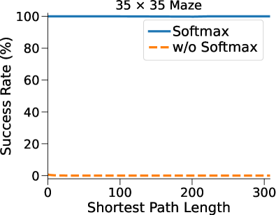
To avoid the gradient exploding problem, we enforce a softmax operation on the values of the latent transition kernel for each latent state $\overline{s}$. This gives a statistical semantic meaning to the latent transition kernel. This change is simple but critical to training stability, as will be shown in experimental results in Section 4.1 and Figure 4(d).

4 Experiments

We perform several experiments to test if our modifications to VIN’s planning module allow training very deep DT-VINs for large-scale long-term planning tasks. In line with previous works (e.g., lee2018gated), we assess our planning algorithms on navigation tasks within 2D mazes and 3D ViZDoom Wydmuch2019ViZDoom environments. Each task includes a start position and a goal position, and the agent navigates the four adjacent cells by moving one step at a time in any of the four cardinal directions. Our experiments look at each method’s effectiveness over several versions of the tasks with the different versions having different shortest path lengths (SPLs). The SPLs are precomputed using Dijkstra’s algorithm and serve as a good proxy measure for the complexity of the planning task. We say that an agent has succeeded in a task if it generates a path from the start position to the goal position within a predetermined number of steps ($m^2$ in our paper). We further say that the agent has found an optimal path if the corresponding path has a minimal length. We follow GPPN and use these for the success rate (SR), which is the rate at which the algorithm succeeds in the task, and the optimality rate (OR), which is the rate at which the algorithm generates an optimal path.

On the above tasks, we compare our DT-VIN method with several advanced neural networks designed for planning tasks, including the original VIN tamar2016value, GPPNs lee2018gated, and Highway VIN wang2024highway. The models are trained through imitation learning using a labelled dataset. We then identify the best-performing model based on its results on a validation dataset and evaluate it on a separate test dataset. Following the methodology from the GPPN paper, we conduct evaluations using three different random seeds for each algorithm. This is sufficient to provide a reliable performance estimate here due to the low standard deviation we observe in the tasks. All figures that show learning curves report the mean and standard deviation on the test set.

4.1 2D Maze Navigation

Setting.

In our evaluation, we use 2D maze navigation tasks with sizes $M$ set to $15$, $25$, $35$, and $100$. Many of these mazes require hundreds or thousands of planning steps to be solved. To assess the performance of each algorithm, we test various neural network depths $N$. Specifically, for mazes of size $M=15$ and $M=25$, we examine depths in $N=30,100,200$. For $M=35$, we examine depths in $N=30,100,300,600$. For the largest mazes, $M=100$, we examine depths of $N=600,5000$, with the exception of GPPN, which is limited to $N=600$ due to GPU resource constraints. For each maze size, we generate a dataset following the methodology in GPPN lee2018gated. Each sample has a starting position, a visual representation of the $m\times m$ map, and an $m\times m$ matrix indicating the position of the goal. For more details, see Section B.1.

Results and Discussion.

Figure 3(a) and Table 1 show the success rates (SRs) of our method and the baseline methods, as a function of the SPLs. For each algorithm and environment configuration, we report the performance of the NN with the best depth $N$ across the ranges specified in the previous paragraph (see Figure 7 in Appendix C for other values of $N$).

Table 1: The success rates for each method under tasks with different ranges of shortest path length. For each algorithm, we choose the best result from a range of depths. Specifically, for our DT-VIN, the optimal depth consistently corresponds to the maximum value in the range: $600$ for size $35$, and $5000$ for size $100$. For other compared methods, the optimal depth differs depending on the task. In the maze of size $100$, the optimal depth for all the baselines is $600$. For additional results, see Figure 7 in Appendix C.

Maze Size	$35\times 35$			$100\times 100$
SPL	[1,100]	[100, 200]	[200, 300]	[1,600]	[600, 1200]	[1200, 1800]
VIN tamar2016value	$68.41\pm 6.25$	$0.00\pm 0.00$	$0.00\pm 0.00$	$45.05\pm 0.04$	$0.00\pm 0.00$	$0.00\pm 0.00$
GPPN lee2018gated	$95.71\pm 0.33$	$0.39\pm 0.27$	$0.00\pm 0.00$	$75.72\pm 0.64$	$0.00\pm 0.00$	$0.00\pm 0.00$
Highway VIN wang2024highway	$90.67\pm 3.92$	$65.50\pm 5.59$	$54.40\pm 10.2$	$69.12\pm 0.02$	$0.00\pm 0.00$	$0.00\pm 0.00$
DT-VIN (ours)	$100.00\pm 0.00$	$99.99\pm 0.01$	$99.77\pm 0.23$	$99.98\pm 0.00$	$99.56\pm 0.20$	$88.65\pm 4.76$

(a)

(b)

Figure 3: SRs and ORs for different algorithms as a function of the shortest path length and the maze size. For each algorithm, we select the best result across various depths. Specifically, for our DT-VIN, the optimal depth consistently corresponds to the maximum value in the range: $200$ for mazes of size $15$ and $25$, $600$ for size $35$, and $5000$ for size $100$. For other methods, the optimal depth differs per task. In the maze of size $100$, the optimal depth for all the baselines is $600$. See Figure 7 and Figure 8 in Appendix C for additional results at other depths.

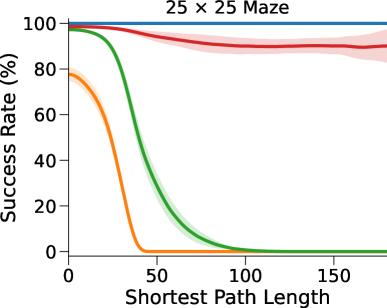
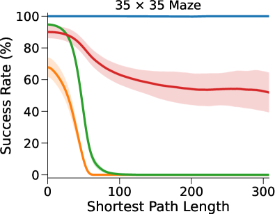
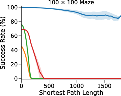
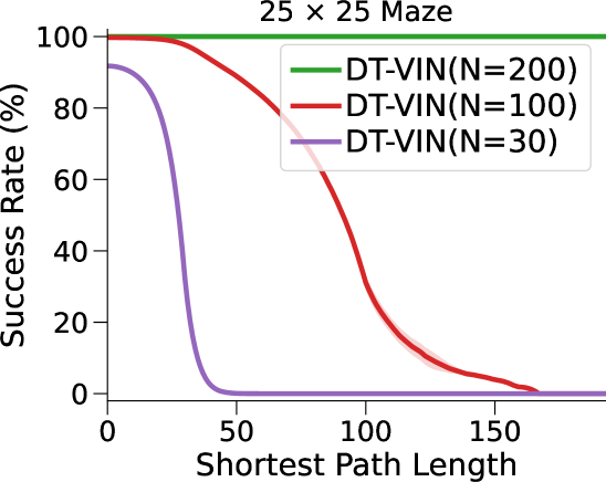
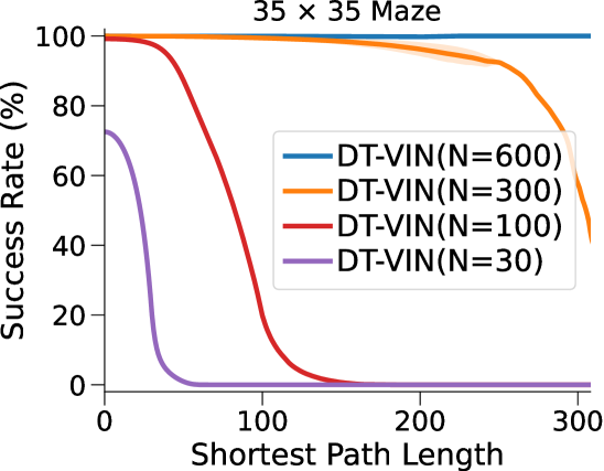
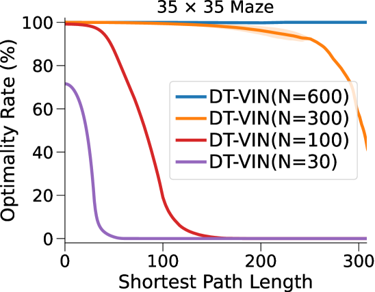
Here, DT-VIN outperforms all the other methods on all the maze navigation tasks under all the various sizes $M$ and SPLs. Notably, on small-scale mazes with size in $M=15,25,35$, DT-VIN achieves approximately 100% SRs on all the tasks. For the most challenging environment with $M=100$, DT-VIN performs best with the full $5000$ layers, and it maintains an SR of approximately 100% on short-term planning tasks with SPL ranging in $[1,200]$ and an SR of approximately 88% on tasks with SPLs over $1200$.

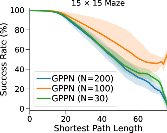
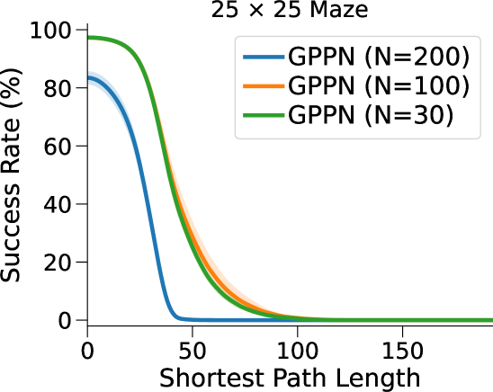
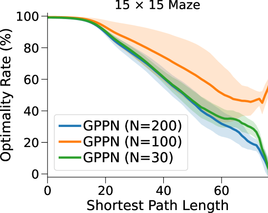
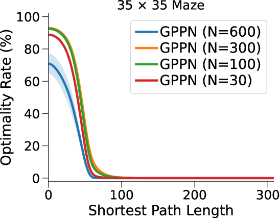
Comparatively, VIN performs well on small-scale and short-term planning tasks. However, even on a small-scale maze with size $M=15$, VIN’s SRs drop to 0% when the SPL exceeds $30$. Moreover, when the maze size increases to $100$, VIN only achieves an SR of less than 40%—even on short-term planning tasks with SPL within $[1,100]$. GPPN performs well on short-term planning tasks, but it fails to generalize well on long-term planning tasks, which also decreases to an SR of 0% as the SPL increases. Highway VIN performs well across tasks with various SPLs on a small-scale maze with $M=15,25$. However, it nevertheless shows a performance decrease on larger-scale maze tasks with $M=35,100$.

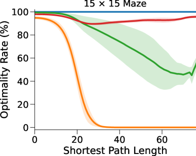
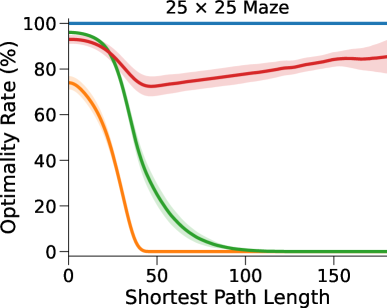
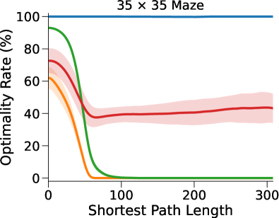
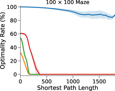
Figure 3(b) shows the optimality rates (ORs) of the algorithms, which measure the rate at which the model outputs the optimal path. Our DT-VIN maintains consistent ORs compared to SRs. However, some other methods—especially Highway VIN—exhibit a clear decrease in ORs, indicating that although these models can generate a path that can achieve the goal, the path is often non-optimal.

Ablation Study.

We perform multiple ablation studies with a $M=35$ maze and an NN with depth $N=600$ to assess the impact on DT-VIN of (1) the dynamic latent transition kernel, as described in Section 3.1; (2) the network depth, as outlined in Section 3.2; (3) the adaptive highway loss, also covered in Section 3.2; and (4) the softmax function on the latent transition kernel, as mentioned in Section 3.2. Unless otherwise mentioned, all these elements are included.

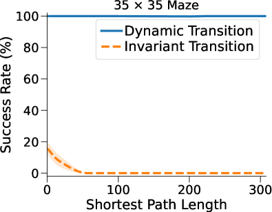
Dynamic Latent Transition Kernel. Figure 4(a) shows the SRs of our method with the proposed dynamic and the original invariant latent transition kernel. The performance with the invariant transition significantly decreases, highlighting the importance of the dynamic transition. It is notable that this variant incorporates the additional adaptive highway loss to the original VIN, which adversely affects the performance when the representation capacity of the latent MDP is limited.

(a)

(b)

(c)

(d)

Figure 4: The results of ablation studies of our DT-VIN with 600 layers. 4(a) shows the performance of DT-VIN using a dynamic versus an invariant latent transition kernel. 4(b) shows the performance of DT-VIN over various depths of the planning module. 4(c) shows the performance of DT-VIN over different loss functions. 4(d) shows the performance of DT-VIN with and without the softmax operation on the latent transition kernel.

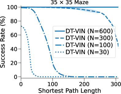
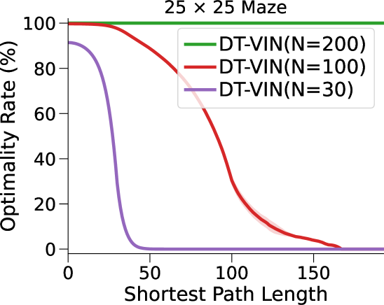
Depth of Planning Module. Figure 4(b) shows the SRs of our DT-VIN with various depths. Here, increasing the depth dramatically enhances the long-term planning ability. For example, for tasks with an SPL of $200$, the variant with depth $N=300$ performs much better than the variant with depth $N=100$. Moreover, for tasks with an SPL of $300$, the deeper variant with depth $N=600$ performs much better. Other methods like VIN and GPPN do not show a clear performance improvement when the depth increases. Figure 7 in Appendix C shows the performance of other methods over all depths.

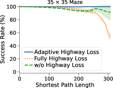
Adaptive Highway Loss. We evaluate two variants of our DT-VIN, the first without the highway loss, and the second with a “fully highway loss,” where the latter enforces a highway loss for each hidden layer without adaptive adjustment based on the actual planning steps. As shown in Figure 4(c), the variant without the highway loss suffers a decrease in performance, and the one with the fully highway loss performs even worse. These results imply that enforcing additional loss on hidden layers without any adjustment could harm performance.

Softmax Latent Transition Kernel. As shown in Figure 4(d), the variant without the softmax operation on the latent transition kernel fails on all the tasks. This failure is due to exploding gradients, wherein the gradient becomes extremely large, eventually resulting in the model’s parameters overflowing and becoming a NaN (Not a Number) value.

4.2 3D ViZDoom Navigation

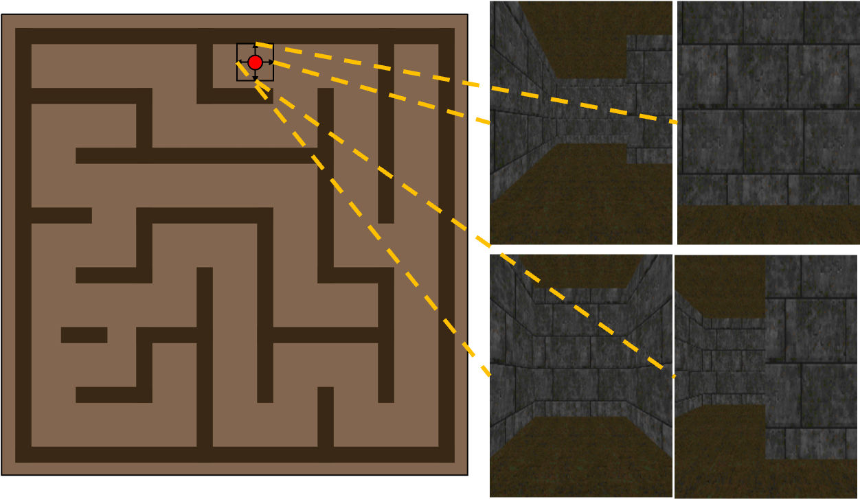
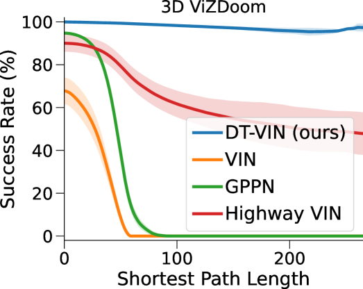
Following the methodology of the GPPN paper, we test our method on 3D ViZDoom Wydmuch2019ViZDoom environments. Here, instead of directly using the top-down 2D maze as in the previous experiments, we use the observation consists of RGB images capturing the first-person perspective of the environment, as illustrated in Figure 5(a). Then, a CNN is trained to predict the maze map from the first-person observation. The map is then given as input to the planning model, using the same architecture and hyperparameters as the 2D maze environments (see Section B.2 for more implementation details). For each algorithm, we select the best result across the various network depths $N=30,100,300,600$. We find that the optimal depth for DT-VIN is $600$, for GPPN is $300$, for VIN is $300$, and for Highway VIN is $300$. Figure 5(b) shows the SRs on 3D ViZDoom mazes with size $M=35$. Predictably, the performance of all the baselines decreases compared to the 2D maze environments due to the additional noise introduced by the predictions. Here, DT-VIN outperforms all the methods compared to the task over all the various SPLs.

(a)

(b)

Figure 5: 5(a) shows an example of a ViZDoom maze and the first-person view of the environment with each of the corresponding four orientations. 5(b) shows the success rates of the algorithms on the 3D ViZDoom environments over various SPLs.

5 Related Work

Variants of Value Iteration Networks (VINs).

Several variants of VIN tamar2016value have been proposed in recent years. Gated Path Planning Networks employ gating recurrent mechanisms to reduce the training instability and hyperparameter sensitivity seen in VINs lee2018gated. To mitigate overestimation bias (which is detrimental to learning here), dVINs were proposed and use a weighted double estimator as an alternative to the maximum operator jin2021value. For addressing challenges in irregular spatial graphs, Generalized VINs adopt a graph convolution operator, extending the traditional convolution operator used in VINs niu2018generalized. To improve scalability, AVINs introduce an abstraction module that extracts higher-level information from the environment and the goal schleich2019value. For transfer learning, Transfer VINs address the generalization of VINs to target domains where the action space or the environment’s features differ from those of the training environments shen2020transfer. More recently, VIRN was proposed and employs larger convolutional kernels to plan using fewer iterations as well as self-attention to propagate information from each layer to the final output of the network cai2022value. Similarly, GS-VIN also uses larger convolutional kernels but to stabilize training and also incorporates a gated summarization module that reduces the accumulated errors during value iteration cai2023value.

Most related to DT-VIN is other recent work that focused on developing very deep VINs for long-term planning. Specifically, Highway VIN wang2024highway incorporates the theory of Highway Reinforcement Learning wang2023highway to create deep planning networks with up to 300 layers for long-term planning tasks. Highway VIN modifies the planning module of VIN by introducing an exploration module that injects stochasticity in the forward pass and uses gating mechanisms to allow selective information flow through the network layers. Our method, however, achieves even deeper planning by incorporating a dynamic transition matrix in the latent MDP and adaptively weighting each layer’s connection to the final output.

Neural Networks with Deep Architectures.

There is a long history of developing very deep neural networks (NNs). For sequential data, this prominently includes the Long Short-Term Memory (LSTM) architecture and its gated residual connections, which help alleviate the “vanishing gradient problem” Hochreiter:97lstm,Hochreiter:91. For feedforward NNs, a similar gated residual connection architecture was used in Highway Networks srivastava2015training and later in the ResNet architecture he2016deep, where the gates were kept open. Such residual connections are still ubiquitous in modern language architectures, such as the Generative Pre-trained Transformer (GPT) achiam2023gpt. Our method dynamically employs skip connections from select hidden layers to the final loss, utilizing a state and observation map-dependent transition kernel. This approach is more closely aligned with the computation of the true VI algorithm. Similar kernels, dependent on an input image chen2020dynamic or the coordinates of an image liu2018intriguing, have been previously used in Computer Vision.

6 Conclusions

Planning is a long-standing challenge in the field of artificial intelligence and its subfield: reinforcement learning. Previous work proposed VIN as an end-to-end differentiable neural network architecture for this task. While VINs have been successful at short-term small-scale planning, they start to fail quite rapidly as the horizon and the scale of the planning grows. We observed that this decay in performance is principally due to limitations in the (1) representational capacity of their network and (2) its depth. To alleviate these problems, we propose several modifications to the architecture, including a dynamic transition kernel to increase the representation capacity and an adaptive highway loss function to ease the training of very deep models. Altogether, these modifications have allowed us to train networks with $5000$ layers. In line with previous work, we evaluate the efficacy of our proposed Dynamic Transition VINs (DT-VINs) on 2D maze environments and 3D ViZDoom environments. We find that DT-VINs scale to exponentially longer-term and exponentially larger-scale planning problems than previous attempts. To the best of our knowledge, DT-VINs is, at the time of publication, the current state-of-the-art planning solution for these specific environments.

We note that the upper bound for this approach (i.e., the scale of the network and, consequentially, the scale of the planning ability) remains unknown. As our experiments were limited mostly by computational cost and not observed instability, we expect that with the growth of available computational power, our method will scale to even longer-term and larger-scale planning.

7 Limitations and Future Work

The principal limitation of our work compared to VIN and Highway VIN is the increased computational cost (see Section B.3). This is a consequence of the scale of the network. The past decades have seen AI dominated by the trend of scaling up systems [sutton2019bitter], so this is not likely a long-term issue. Other limitations include the requirement to know the length of the shortest path $l$ in the highway loss. In a general RL problem, such a quantity could be estimated online. Future work will explore the impact of a more sophisticated transition mapping module (this work uses a single CNN layer for this purpose) in more challenging real-world applications, such as real-time robotics navigation in dynamic and unpredictable environments.

Appendix A Broad Impact

Our work principally involves fundamental research and does not have a clear negative societal impact in excess of those held by all scientific advancements.

Appendix B Experimental Details

The below subsections detail specific information about the experiments that have been deemed too minor to appear in the main text.

B.1 2D Maze Navigation

Figure 6 shows some visualizations of some of the different 2D maze navigation tasks we experiment with. Our experimental setup follows the guidelines established in the GPPN paper lee2018gated. For these tasks, the datasets for training, validation, and testing comprise $25000$, $5000$, and $5000$ mazes, respectively. Each maze features a goal position, with all reachable positions selected as potential starting points. Note that this setting, as done by GPPN, produces a distribution of mazes with non-uniform SPLs, which is skewed towards shorter SPLs. Table 2 shows the hyperparameters used by our method. Note that, while DT-VIN consistently uses $3$ for the size of the latent transition kernel $F$ and $4$ for the size of the latent action space $|\overline{𝒜}|$, other methods instead used their best-performing sizes from between $3$ and $5$, and between $4$ and $150$, respectively.

B.2 3D ViZDoom

To be in line with previous work, we use a state representation preprocessing stage for the 3D ViZDoom environment similar to that used in the GPPN paper and others lee2018gated, lample2017playing. Specifically, for each point in the $M\times M$ 3D maze, the RGB first-person views for each of the four cardinal directions are given as state to a preprocessing network (see Figure 5(a)). This network then encodes this state and produces an $M\times M$ binary maze matrix. The hyperparameters and exact specification of the network are given in Table 3.

B.3 Computational Complexity

As we have discussed in Section 3.1, our approaches only require $|\overline{𝒜}|\times F^4$ parameters, where we set $|\overline{𝒜}|=4$ and $F=3$ in our experiments. Table 4, shows the GPU memory consumption and training time on an NVIDIA A100 GPU for DT-VIN and the baselines when using $600$ layers and training for 30 epochs $35\times 35$ maze.

(a)

(b)

(c)

(d)

Figure 6: Some examples of the 2D maze navigation tasks.

Table 2: 2D Maze Navigation Hyperparameters

Hyperparameter	Value
Transition Mapping Module	Conv with $3\times 3$ kernel
Reward Mapping Module	Conv with $1\times 1$ kernel
Latent Transition Kernel Size ($F$)	3
Latent Action Space Size ($|\overline{𝒜}|$)	4
Optimizer	RMSprop
Learning Rate	1e-3
Batch Size	32
Skip Size for Adaptive Highway Loss $l_j$	10
Depth of Planning Module	$15\times 15$ maze: $200$ $25\times 25$ maze: $200$ $35\times 35$ maze: $600$ $100\times 100$ maze: $5000$

Table 3: 3D ViZDoom Preprocessing Network

Hyperparameter	Value
Batch Size ($B$)	32
Image Directions ($D$)	4
Image Channels ($C$)	3
Image Width ($W$)	24
Image Height ($H$)	32
Input Size	$(B,M,M,D,W,H,C)$
Layer 1 (Convolution)	$(3,32,8,4,1)$
Layer 2 (Convolution)	$(32,64,4,2,1)$
Layer 3 (Linear)	$(384,256)$
Layer 4 (Convolution)	$(1024,64,3,1,1)$
Layer 5 (Convolution)	$(64,1,3,1,1)$
Output Size	$(B,M,M)$
Optimizer	Adam
Learning Rate	1e-3
Betas	$(0.9,0.999)$

Table 4: Compuational Complexity

Method	GPU Memory (GB)	Training Time (hours)
VIN	4.2	8.4
GPPN	182	4.2
Highway VIN	41.3	14.3
DT-VIN	53.3	12.1

Appendix C Additional Experimental Results

Due to space constraints, the below results could not appear in the main text. Figure 7 shows the success rate of all the algorithms on the $15\times 15$, $25\times 25$, and $35\times 35$ mazes as a function of the shortest path length and the depth of the network. Similarly, Figure 8 shows the corresponding optimality rates.

(a)

(b)

(c)

Figure 7: The success rate of each method as a function of shortest path length and network depth. The green and red curves overlap in the top-left plot.

(a)

(b)

(c)

Figure 8: The optimality rate of each method as a function of shortest path length and network depth. The green and red curves overlap in the top-left plot.