Step-by-Step Diffusion: An Elementary Tutorial

Abstract

We present an accessible first course on diffusion models and flow matching for machine learning, aimed at a technical audience with no diffusion experience. We try to simplify the mathematical details as much as possible (sometimes heuristically), while retaining enough precision to derive correct algorithms.

Preface

There are many existing resources for learning diffusion models. Why did we write another? Our goal was to teach diffusion as simply as possible, with minimal mathematical and machine learning prerequisites, but in enough detail to reason about its correctness. Unlike most tutorials on this subject, we take neither a Variational Auto Encoder (VAE) nor an Stochastic Differential Equations (SDE) approach. In fact, for the core ideas we will not need any SDEs, Evidence-Based-Lower-Bounds (ELBOs), Langevin dynamics, or even the notion of a score. The reader need only be familiar with basic probability, calculus, linear algebra, and multivariate Gaussians. The intended audience for this tutorial is technical readers at the level of at least advanced undergraduate or graduate students, who are learning diffusion for the first time and want a mathematical understanding of the subject.

This tutorial has five parts, each relatively self-contained, but covering closely related topics. Section 1 presents the fundamentals of diffusion: the problem we are trying to solve and an overview of the basic approach. Sections 2 and 3 show how to construct a stochastic and deterministic diffusion sampler, respectively, and give intuitive derivations for why these samplers correctly reverse the forward diffusion process. Section 4 covers the closely-related topic of Flow Matching, which can be thought of as a generalization of diffusion that offers additional flexibility (including what are called rectified flows or linear flows). Finally, in Section 5 we return to diffusion and connect this tutorial to the broader literature while highlighting some of the design choices that matter most in practice, including samplers, noise schedules, and parametrizations.

Acknowledgements

We are grateful for helpful feedback and suggestions from many people, in particular: Josh Susskind, Eugene Ndiaye, Dan Busbridge, Sam Power, De Wang, Russ Webb, Sitan Chen, Vimal Thilak, Etai Littwin, Chenyang Yuan, Alex Schwing, and Miguel Angel Bautista Martin.

1 Fundamentals of Diffusion

The goal of generative modeling is: given i.i.d. samples from some unknown distribution $p^{\ast }\left(x\right)$, construct a sampler for (approximately) the same distribution. For example, given a training set of dog images from some underlying distribution $p_{\text{dog}}$, we want a method of producing new images of dogs from this distribution.

One way to solve this problem, at a high level, is to learn a transformation from some easy-to-sample distribution (such as Gaussian noise) to our target distribution $p^{\ast }$. Diffusion models offer a general framework for learning such transformations. The clever trick of diffusion is to reduce the problem of sampling from distribution $p^{\ast }\left(x\right)$ into to a sequence of easier sampling problems.

This idea is best explained via the following Gaussian diffusion example. We’ll sketch the main ideas now, and in later sections we will use this setup to derive what are commonly known as the DDPM and DDIM samplers, and reason about their correctness.

1.1 Gaussian Diffusion

For Gaussian diffusion, let $x_0$ be a random variable in ${ℝ}^d$ distributed according to the target distribution $p^{\ast }$ (e.g., images of dogs). Then construct a sequence of random variables $x_1,x_2,\mathrm{\dots },x_T$, by successively adding independent Gaussian noise with some small scale $\sigma$:

$$x_{t+1}:=x_t+{\eta }_t,{\eta }_t\sim 𝒩(0,{\sigma }^2).$$ (1)

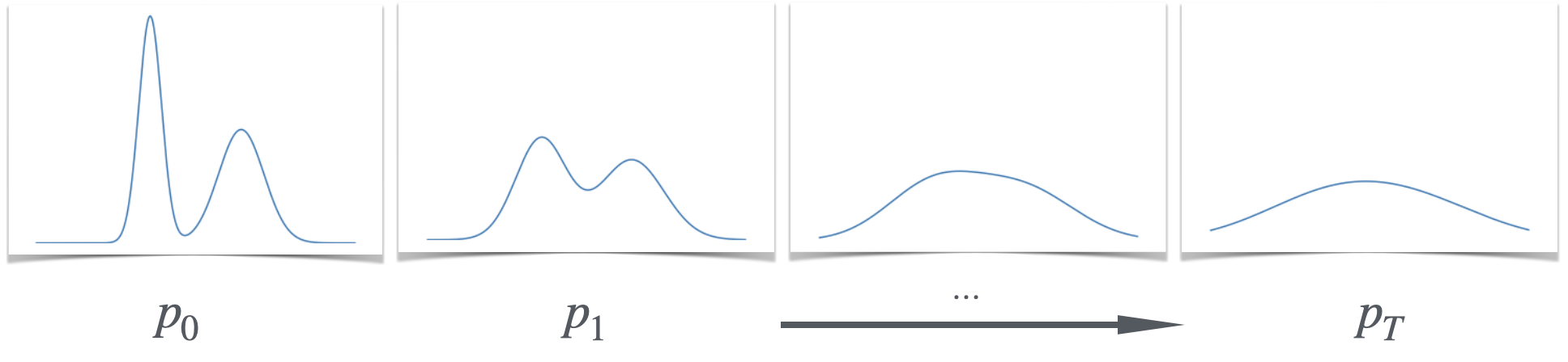
This is called the forward process, which transforms the data distribution into a noise distribution. Equation (1) defines a joint distribution over all $(x_0,x_1,\mathrm{\dots },x_T)$, and we let ${\left\{p_t\right\}}_{t\in \left[T\right]}$ denote the marginal distributions of each $x_t$. Notice that at large step count $T$, the distribution $p_T$ is nearly Gaussian, so we can approximately sample from $p_T$ by just sampling a Gaussian.

Figure 1: Probability distributions defined by diffusion forward process on one-dimensional target distribution $p_0$.

Now, suppose we can solve the following subproblem:

“Given a sample marginally distributed as ${\mathrm{p}}_{\mathrm{t}}$, produce a sample marginally distributed as ${\mathrm{p}}_{\mathrm{t}-1}$”.

We will call a method that does this a reverse sampler, since it tells us how to sample from $p_{t-1}$ assuming we can already sample from $p_t$. If we had a reverse sampler, we could sample from our target $p_0$ by simply starting with a Gaussian sample from $p_T$, and iteratively applying the reverse sampling procedure to get samples from $p_{T-1},p_{T-2},\mathbf{\dots }$ and finally $p_0=p^{\ast }$.

The key insight of diffusion is, learning to reverse each intermediate step can be easier than learning to sample from the target distribution in one step. There are many ways to construct reverse samplers, but for concreteness let us first see the standard diffusion sampler which we will call the DDPM sampler.k

The Ideal DDPM sampler uses the obvious strategy: At time $t$, given input $z$ (which is promised to be a sample from $p_t$), we output a sample from the conditional distribution

$$p\left(x_{t-1}\mid x_t=z\right).$$ (2)

This is clearly a correct reverse sampler. The problem is, it requires learning a generative model for the conditional distribution $p\left(x_{t-1}\mid x_t\right)$ for every $x_t$, which could be complicated. But if the per-step noise $\sigma$ is sufficiently small, then it turns out this conditional distribution becomes simple:

Figure 2: Illustration of Fact 1. The prior distribution $p(x_{t-1})$, leftmost, defines a joint distribution $(x_{t-1},x_t)$ where $p(x_t\mid x_{t-1})=𝒩(0,{\sigma }^2)$. We plot the reverse conditional distributions $p(x_{t-1}\mid x_t)$ for a fixed conditioning $x_t$, and varying noise levels $\sigma$. Notice these distributions become close to Gaussian for small $\sigma$.

Fact 1 (Diffusion Reverse Process).

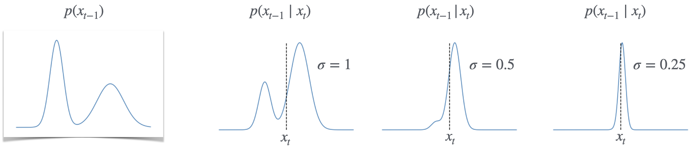
For small $\sigma$, and the Gaussian diffusion process defined in (1), the conditional distribution $p(x_{t-1}\mid x_t)$ is itself close to Gaussian. That is, for all times $t$ and conditionings $z\in {ℝ}^d$, there exists some mean parameter $\mu \in {ℝ}^d$ such that

$$p\left(x_{t-1}\mid x_t=z\right)\approx 𝒩(x_{t-1};\mu ,{\sigma }^2).$$ (3)

This is not an obvious fact; we will derive it in Section 2.1. This fact enables a drastic simplification: instead of having to learn an arbitrary distribution $p\left(x_{t-1}\mid x_t\right)$ from scratch, we now know everything about this distribution except its mean, which we denote ${\mu }_{t-1}\left(x_t\right)$. The fact that we can approximate the posterior distribution as Gaussian when $\sigma$ is sufficiently small is illustrated in Fig 2. This is an important point, so to re-iterate: for a given time $t$ and conditioning value $x_t$, learning the mean of $p\left(x_{t-1}\mid x_t\right)$ is sufficient to learn the full conditional distribution $p\left(x_{t-1}\mid x_t\right)$.

Learning the mean of $p\left(x_{t-1}\mid x_t\right)$ is a much simpler problem than learning the full conditional distribution, because we can solve it by regression. To elaborate, we have a joint distribution $(x_{t-1},x_t)$ from which we can easily sample, and we would like to estimate $𝔼\left[x_{t-1}\mid x_t\right]$. This can be done by optimizing a standard regression loss:

${\mu }_{t-1}\left(z\right)$ $:=𝔼\left[x_{t-1}\mid x_t=z\right]$ (4)

$⟹{\mu }_{t-1}$ $=\underset{f:{ℝ}^d\to {ℝ}^d}{argmin}\underset{x_t,x_{t-1}}{𝔼}{\Vert f\left(x_t\right)-x_{t-1}\Vert }_2^2$ (5)

$=\underset{f:{ℝ}^d\to {ℝ}^d}{argmin}\underset{x_{t-1},\eta }{𝔼}\left|\right|f(x_{t-1}+{\eta }_t)-x_{t-1}\left)\right||{}_2{}^2,$ (6)

where the expectation is taken over samples $x_0$ from our target distribution $p^{\ast }$. This particular regression problem is well-studied in certain settings. For example, when the target $p^{\ast }$ is a distribution on images, then the corresponding regression problem (Equation 6) is exactly an image denoising objective, which can be approached with familiar methods (e.g. convolutional neural networks).

Stepping back, we have seen something remarkable: we have reduced the problem of learning to sample from an arbitrary distribution to the standard problem of regression.

1.2 Diffusions in the Abstract

Let us now abstract away the Gaussian setting, to define diffusion-like models in a way that will capture their many instantiations (including deterministic samplers, discrete domains, and flow-matching).

Abstractly, here is how to construct a diffusion-like generative model: We start with our target distribution $p^{\ast }$, and we pick some base distribution $q\left(x\right)$ which is easy to sample from, e.g. a standard Gaussian or i.i.d bits. We then try to construct a sequence of distributions which interpolate between our target $p^{\ast }$ and the base distribution $q$. That is, we construct distributions

$$p_0,p_1,p_2,\mathrm{\dots },p_T,$$ (7)

such that $p_0=p^{\ast }$ is our target, $p_T=q$ the base distribution, and adjacent distributions $(p_{t-1},p_t)$ are marginally “close” in some appropriate sense. Then, we learn a reverse sampler which transforms distributions $p_t$ to $p_{t-1}$. This is the key learning step, which presumably is made easier by the fact that adjacent distributions are “close.” Formally, reverse samplers are defined below.

Definition 1 (Reverse Sampler).

Given a sequence of marginal distributions $p_t$, a reverse sampler for step $t$ is a potentially stochastic function $F_t$ such that if $x_t\sim p_t$, then the marginal distribution of $F_t(x_t)$ is exactly $p_{t-1}$:

$$\{F_t\left(z\right):z\sim p_t\}\equiv p_{t-1}.$$ (8)

There are many possible reverse samplers, and it is even possible to construct reverse samplers which are deterministic. In the remainder of this tutorial we will see three popular reverse samplers more formally: the DDPM sampler discussed above (Section 2.1), the DDIM sampler (Section 3), which is deterministic, and the family of flow-matching models (Section 4), which can be thought of as a generalization of DDIM.

1.3 Discretization

Before we proceed further, we need to be more precise about what we mean by adjacent distributions $p_t,p_{t-1}$ being “close”. We want to think of the sequence $p_0,p_1,\mathrm{\dots },p_T$ as the discretization of some (well-behaved) time-evolving function $p(x,t)$, that starts from the target distribution $p_0$ at time $t=0$ and ends at the noisy distribution $p_T$ at time $t=1$:

$$p(x,k\mathrm{\Delta }t)=p_k\left(x\right),\text{where}\mathrm{\Delta }t=\frac{1}{T}.$$ (9)

The number of steps $T$ controls the fineness of the discretization (hence the closeness of adjacent distributions).

In order to ensure that the variance of the final distribution, $p_T$, is independent of the number of discretization steps, we also need to be more specific about the variance of each increment. Note that if $x_k=x_{k-1}+𝒩(0,{\sigma }^2)$, then $x_T\sim 𝒩(x_0,T{\sigma }^2)$. Therefore, we need to scale the variance of each increment by $\mathrm{\Delta }t=1/T$, that is, choose

$\sigma ={\sigma }_q\sqrt{\mathrm{\Delta }t},$ (10)

where ${\sigma }_q^2$ is the desired terminal variance. This choice ensures that the variance of $p_T$ is always ${\sigma }_q^2$, regardless of $T$. (The $\sqrt{\mathrm{\Delta }t}$ scaling will turn out to be important in our arguments for the correctness of our reverse solvers in the next chapter, and also connects to the SDE formulation in Section 2.4.)

At this point, it is convenient to adjust our notation. From here on, $t$ will represent a continuous-value in the interval $[0,1]$ (specifically, taking one of the values $0,\mathrm{\Delta }t,2\mathrm{\Delta }t,\mathrm{\dots },T\mathrm{\Delta }t=1$). Subscripts will indicate time rather than index, so for example $x_t$ will now denote $x$ at a discretized time $t$. That is, Equation 1 becomes:

$$x_{t+\mathrm{\Delta }t}:=x_t+{\eta }_t,{\eta }_t\sim 𝒩(0,{\sigma }_q^2\mathrm{\Delta }t),$$ (11)

which also implies that

$$x_t\sim 𝒩(x_0,{\sigma }_t^2),\text{where}{\sigma }_t:={\sigma }_q\sqrt{t},$$ (12)

since the total noise added up to time $t$ (i.e. ${\sum }_{\tau \in \{0,\mathrm{\Delta }t,2\mathrm{\Delta }t,\mathrm{\dots },t-\mathrm{\Delta }t\}}{\eta }_{\tau }$) is also Gaussian with mean zero and variance ${\sum }_{\tau }{\sigma }_q^2\mathrm{\Delta }t={\sigma }_q^{2}t$.

2 Stochastic Sampling: DDPM

In this section we review the DDPM-like reverse sampler discussed in Section 1, and heuristically prove its correctness. This sampler is conceptually the same as the sampler popularized in Denoising Diffusion Probabilistic Models (DDPM) by Ho et al. (2020) and originally introduced by Sohl-Dickstein et al. (2015), when adapted to our simplified setting. However, a word of warning for the reader familiar with Ho et al. (2020): Although the overall strategy of our sampler is identical to Ho et al. (2020), certain technical details (like constants, etc) are slightly different.

We consider the setup from Section 1.3, with some target distribution $p^{\ast }$ and the joint distribution of noisy samples $(x_0,x_{\mathrm{\Delta }t},\mathrm{\dots },x_1)$ defined by Equation (11). The DDPM sampler will require estimates of the following conditional expectations:

${\mu }_t\left(z\right):=𝔼\left[x_t\mid x_{t+\mathrm{\Delta }t}=z\right].$ (13)

This is a set of functions $\left\{{\mu }_t\right\}$, one for every time step $t\in \{0,\mathrm{\Delta }t,\mathrm{\dots },1-\mathrm{\Delta }t\}$. In the training phase, we estimate these functions from i.i.d. samples of $x_0$, by optimizing the denoising regression objective

${\mu }_t$ $=\underset{f:{ℝ}^d\to {ℝ}^d}{argmin}\underset{x_t,x_{t+\mathrm{\Delta }t}}{𝔼}{\Vert f\left(x_{t+\mathrm{\Delta }t}\right)-x_t\Vert }_2^2,$ (14)

typically with a neural-network parameterizing $f$. Then, in the inference phase, we use the estimated functions in the following reverse sampler.

[nobreak=true] Algorithm 1: Stochastic Reverse Sampler (DDPM-like)
For input sample $x_t$, and timestep $t$, output:

${\widehat{x}}_{t-\mathrm{\Delta }t}\leftarrow {\mu }_{t-\mathrm{\Delta }t}\left(x_t\right)+𝒩(0,{\sigma }_q^2\mathrm{\Delta }t)$ (15)

To actually generate a sample, we first sample $x_1$ as an isotropic Gaussian $x_1\sim 𝒩(0,{\sigma }_q^2)$, and then run the iteration of Algorithm 1 down to $t=0$, to produce a generated sample ${\widehat{x}}_0$. (Recall that in our discretized notation (12), $x_1$ is the fully-noised terminal distribution, and the iteration takes steps of size $\mathrm{\Delta }t$.) Explicit pseudocode for these algorithms are given in Section 2.2.

We want to reason about correctness of this entire procedure: why does iterating Algorithm 1 produce a sample from [approximately] our target distribution $p^{\ast }$? The key missing piece is, we need to prove some version of Fact 1: that the true conditional $p\left(x_{t-\mathrm{\Delta }t}\mid x_t\right)$ can be well-approximated by a Gaussian, and this approximation gets better as we scale $\mathrm{\Delta }t\to 0$.

2.1 Correctness of DDPM

Here is a more precise version of Fact 1, along with a heuristic derivation. This will complete the argument that Algorithm 1 is correct— i.e. that it approximates a valid reverse sampler in the sense of Definition 1.

Claim 1 (Informal).

Let $p_{t-\mathrm{\Delta }t}(x)$ be an arbitrary, sufficiently-smooth density over ${ℝ}^d$. Consider the joint distribution of $(x_{t-\mathrm{\Delta }t},x_t)$, where $x_{t-\mathrm{\Delta }t}\sim p_{t-\mathrm{\Delta }t}$ and $x_t\sim x_{t-\mathrm{\Delta }t}+𝒩(0,{\sigma }_q^2\mathrm{\Delta }t)$. Then, for sufficiently small $\mathrm{\Delta }t$, the following holds. For all conditionings $z\in {ℝ}^d$, there exists ${\mu }_z$ such that:

$p\left(x_{t-\mathrm{\Delta }t}\mid x_t=z\right)\approx 𝒩(x_{t-\mathrm{\Delta }t};{\mu }_z,{\sigma }_q^2\mathrm{\Delta }t).$ (16)

for some constant ${\mu }_z$ depending only on $z$. Moreover, it suffices to take

${\mu }_z$ $:=\underset{(x_{t-\mathrm{\Delta }t},x_t)}{𝔼}\left[x_{t-\mathrm{\Delta }t}\mid x_t=z\right]$ (17)

$=z+\left({\sigma }_q^2\mathrm{\Delta }t\right)\nabla \log p_t\left(z\right),$ (18)

where $p_t$ is the marginal distribution of $x_t$.

Before we see the derivation, a few remarks: Claim 1 implies that to sample from $x_{t-\mathrm{\Delta }t}$, it suffices to first sample from $x_t$, then sample from a Gaussian distribution centered around $𝔼\left[x_{t-\mathrm{\Delta }t}\mid x_t\right]$. This is exactly what DDPM does, in Equation (15). Finally, in these notes we will not actually need the expression for ${\mu }_z$ in Equation (18); it is enough for us know that such a ${\mu }_z$ exists, so we can learn it from samples.

Proof of Claim 1 (Informal).

Here is a heuristic argument for why the score appears in the reverse process. We will essentially just apply Bayes rule and then Taylor expand appropriately. We start with Bayes rule:

$p\left(x_{t-\mathrm{\Delta }t}|x_t\right)$ $=p\left(x_t|x_{t-\mathrm{\Delta }t}\right)p_{t-\mathrm{\Delta }t}\left(x_{t-\mathrm{\Delta }t}\right)/p_t\left(x_t\right)$ (19)

Then take logs of both sizes. Throughout, we will drop any additive constants in the log (which translate to normalizing factors), and drop all terms of order $𝒪(\mathrm{\Delta }t)$ -1cm]Note that $x_{t+1}-x_t\sim 𝒪(\sqrt{\mathrm{\Delta }t})$. Dropping $𝒪(\mathrm{\Delta }t)$ terms means dropping ${(x_{t+1}-x_t)}^2\sim 𝒪(\mathrm{\Delta }t)$ in the expansion of $p_t(x_t)$, but keeping $\frac{1}{2{\sigma }_q^2\mathrm{\Delta }t}{(x_{t+1}-x_t)}^2\sim 𝒪(1)$ in $p(x_t|x_{t+1})$.. Note that we should think of $x_t$ as a constant in this derivation, since we want to understand the conditional probability as a function of $x_{t-\mathrm{\Delta }t}$. Now:

$\log p\left(x_{t-\mathrm{\Delta }t}|x_t\right)=\log p\left(x_t|x_{t-\mathrm{\Delta }t}\right)+\log p_{t-\mathrm{\Delta }t}\left(x_{t-\mathrm{\Delta }t}\right)\cancel{-\log p_t\left(x_t\right)}$ Drop constants involving only $x_t$.

$=\log p\left(x_t|x_{t-\mathrm{\Delta }t}\right)+\log p_t\left(x_{t-\mathrm{\Delta }t}\right)+𝒪\left(\mathrm{\Delta }t\right)$ Since $p_{t-\mathrm{\Delta }t}(\cdot )=p_t(\cdot )+\mathrm{\Delta }t\frac{\partial }{\partial t}{p}_t(\cdot )$.

$=-{\displaystyle \frac{1}{2{\sigma }_q^2\mathrm{\Delta }t}}{\Vert x_{t-\mathrm{\Delta }t}-x_t\Vert }_2^2+\log p_t\left(x_{t-\mathrm{\Delta }t}\right)$ Definition of $\log p(x_t|x_{t-\mathrm{\Delta }t})$.

$=-{\displaystyle \frac{1}{2{\sigma }_q^2\mathrm{\Delta }t}}{\Vert x_{t-\mathrm{\Delta }t}-x_t\Vert }_2^2$

$+\cancel{\log p_t\left(x_t\right)}+⟨{\nabla }_x\log p_t\left(x_t\right),\left(x_{t-\mathrm{\Delta }t}-x_t\right)⟩+𝒪\left(\mathrm{\Delta }t\right)$ Taylor expand around $x_t$ and drop constants.

$=-{\displaystyle \frac{1}{2{\sigma }_q^2\mathrm{\Delta }t}}\left({\Vert x_{t-\mathrm{\Delta }t}-x_t\Vert }_2^2-2{\sigma }_q^2\mathrm{\Delta }t⟨{\nabla }_x\log p_t\left(x_t\right),\left(x_{t-\mathrm{\Delta }t}-x_t\right)⟩\right)$

$=-{\displaystyle \frac{1}{2{\sigma }_q^2\mathrm{\Delta }t}}{\Vert x_{t-\mathrm{\Delta }t}-x_t-{\sigma }_q^2\mathrm{\Delta }t{\nabla }_x\log p_t\left(x_t\right)\Vert }_2^2+C$ Complete the square in $(x_{t-\mathrm{\Delta }t}-x_t)$, and drop constant $C$ involving only $x_t$.

$=-{\displaystyle \frac{1}{2{\sigma }_q^2\mathrm{\Delta }t}}{\Vert x_{t-\mathrm{\Delta }t}-\mu \Vert }_2^2$ For $\mu :=x_t+({\sigma }_q^2\mathrm{\Delta }t){\nabla }_x\log p_t(x_t)$.

This is identical, up to additive factors, to the log-density of a Normal distribution with mean $\mu$ and variance ${\sigma }_q^2\mathrm{\Delta }t$. Therefore,

$$p\left(x_{t-\mathrm{\Delta }t}\mid x_t\right)\approx 𝒩(x_{t-\mathrm{\Delta }t};\mu ,{\sigma }_q^2\mathrm{\Delta }t).$$ (20)

∎

Reflecting on this derivation, the main idea was that for small enough $\mathrm{\Delta }t$, the Bayes-rule expansion of the reverse process $p\left(x_{t-\mathrm{\Delta }t}\mid x_t\right)$ is dominated by the term $p\left(x_t\mid x_{t-\mathrm{\Delta }t}\right)$, from the forward process. This is intuitively why the reverse process and the forward process have the same functional form (both are Gaussian here).

Technical Details [Optional].

The meticulous reader may notice that Claim 1 is not obviously sufficient to imply correctness of the entire DDPM algorithm. The issue is: as we scale down $\mathrm{\Delta }t$, the error in our per-step approximation (Equation 16) decreases, but the number of total steps required increases. So if the per-step error does not decrease fast enough (as a function of $\mathrm{\Delta }t$), then these errors could accumulate to a non-negligible error by the final step. Thus, we need to quantify how fast the per-step error decays. Lemma 1 below is one way of quantifying this: it states that if the step-size (i.e. variance of the per-step noise) is ${\sigma }^2$, then the KL error of the per-step Gaussian approximation is $𝒪\left({\sigma }^4\right)$. This decay rate is fast enough, because the number of steps only grows as $\mathrm{\Omega }\left(1/{\sigma }^2\right)$.

Lemma 1.

Let $p(x)$ be an arbitrary density over $ℝ$, with bounded 1st to 4th order derivatives. Consider the joint distribution $(x_0,x_1)$, where $x_0\sim p$ and $x_1\sim x_0+𝒩(0,{\sigma }^2)$. Then, for any conditioning $z\in ℝ$, we have

$$\mathrm{KL}\left(𝒩({\mu }_z,{\sigma }^2)\right|\left|p_{x_0\mid x_1}(\cdot \mid x_1=z)\right)\le O\left({\sigma }^4\right),$$ (21)

where

$${\mu }_z:=z+{\sigma }^2\nabla \log p\left(z\right).$$ (22)

It is possible to prove Lemma 1 by doing essentially a careful Taylor expansion; we include the full proof in Appendix B.1.

2.2 Algorithms

Pseudocode listings 1 and 2 give the explicit DDPM train loss and sampling code. To train the network $f_{\theta }$, we must minimize the expected loss $L_{\theta }$ output by Pseudocode 1, typically by backpropagation.

Pseudocode 3 describes the closely-related DDIM sampler, which will be discussed later in Section 3.

Input: Neural network $f_{\theta }$; Sample-access to target distribution $p$.

Data: Terminal variance ${\sigma }_q$; step-size $\mathrm{\Delta }t$.

Output: Stochastic loss $L_{\theta }$

1 $x_0\leftarrow \text{Sample}\left(p\right)$

2 $t\leftarrow \text{Unif}[0,1]$

3 $x_t\leftarrow x_0+𝒩(0,{\sigma }_q^{2}t)$

4 $x_{t+\mathrm{\Delta }t}\leftarrow x_t+𝒩(0,{\sigma }_q^2\mathrm{\Delta }t)$

5 $L\leftarrow {\Vert f_{\theta }(x_{t+\mathrm{\Delta }t},t+\mathrm{\Delta }t)-x_t\Vert }_2^2$

return $L_{\theta }$

Pseudocode 1 DDPM train loss

Input: Trained model $f_{\theta }$.

Data: Terminal variance ${\sigma }_q$; step-size $\mathrm{\Delta }t$.

Output: $x_0$

1 $x_1\leftarrow 𝒩(0,{\sigma }_q^2)$

2 for $t=1,(1-\mathrm{\Delta }t),(1-2\mathrm{\Delta }t),\mathrm{\dots },\mathrm{\Delta }t$ do

3 $\eta \leftarrow 𝒩(0,{\sigma }_q^2\mathrm{\Delta }t)$

4 $x_{t-\mathrm{\Delta }t}\leftarrow f_{\theta }(x_t,t)+\eta$

5

6 end for

return $x_0$

Pseudocode 2 DDPM sampling (Code for Algorithm 1)

Input: Trained model $f_{\theta }$

Data: Terminal variance ${\sigma }_q$; step-size $\mathrm{\Delta }t$.

Output: $x_0$

1 $x_1\leftarrow 𝒩(0,{\sigma }_q^2)$

2 for $t=1,(1-\mathrm{\Delta }t),(1-2\mathrm{\Delta }t),\mathrm{\dots },\mathrm{\Delta }t,0$ do

3 $\lambda \leftarrow \frac{\sqrt{t}}{\sqrt{t-\mathrm{\Delta }t}+\sqrt{t}}$

4 $x_{t-\mathrm{\Delta }t}\leftarrow x_t+\lambda \left(f_{\theta }(x_t,t)-x_t\right)$

5

6 end for

return $x_0$

Pseudocode 3 DDIM sampling (Code for Algorithm 2)

2.3 Variance Reduction: Predicting $x_0$

Thus far, our diffusion models have been trained to predict $𝔼[x_{t-\mathrm{\Delta }t}\mid x_t]$: this is what Algorithm 1 requires, and what the training procedure of Pseudocode 1 produces. However, many practical diffusion implementations actually train to predict $𝔼\left[x_0\mid x_t\right]$, i.e. to predict the expectation of the initial point $x_0$ instead of the previous point $x_{t-\mathrm{\Delta }t}$. This difference turns out to be just a variance reduction trick, which estimates the same quantity in expectation. Formally, the two quantities can be related as follows:

Claim 2.

For the Gaussian diffusion setting of Section 1.3 , we have:

$𝔼\left[\left(x_{t-\mathrm{\Delta }t}-x_t\right)\mid x_t\right]={\displaystyle \frac{\mathrm{\Delta }t}{t}}𝔼\left[\left(x_0-x_t\right)\mid x_t\right].$ (23)

Or equivalently:

$$𝔼\left[x_{t-\mathrm{\Delta }t}\mid x_t\right]=\left(\frac{\mathrm{\Delta }t}{t}\right)𝔼\left[x_0\mid x_t\right]+\left(1-\frac{\mathrm{\Delta }t}{t}\right)x_t.$$ (24)

This claim implies that if we want to estimate $𝔼\left[x_{t-\mathrm{\Delta }t}\mid x_t\right]$, we can instead estimate $𝔼\left[x_0\mid x_t\right]$ and then then essentially divide by $\left(t/\mathrm{\Delta }t\right)$, which is the number of steps taken thus far. The variance-reduced versions of the DDPM training and sampling algorithms do exactly this; we include them in Appendix B.9.

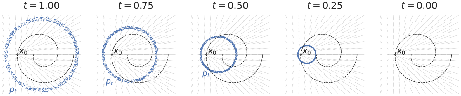
The intuition behind Claim 2. Given $x_t$, the final noise step ${\eta }_{t-\mathrm{\Delta }t}$ is distributed identically as all other noise steps, intuitively because we only know the sum $x_t=x_0+{\sum }_i{\eta }_i$. The intuition behind Claim 2 is illustrated in Figure 2: first, observe that predicting $x_{t-\mathrm{\Delta }t}$ given $x_t$ is equivalent to predicting the last noise step, which is ${\eta }_{t-\mathrm{\Delta }t}=\left(x_t-x_{t-\mathrm{\Delta }t}\right)$ in the forward process of Equation (11). But, if we are only given the final $x_t$, then all of the previous noise steps intuitively “look the same”— we cannot distinguish between noise that was added at the last step from noise that was added at the 5th step, for example. By this symmetry, we can conclude that all of the individual noise steps are distributed identically (though not independently) given $x_t$. Thus, instead of estimating a single noise step, we can equivalently estimate the average of all prior noise steps, which has much lower variance. There are $\left(t/\mathrm{\Delta }t\right)$ elapsed noise steps by time $t$, so we divide the total noise by this quantity in Equation 23 to compute the average. See Appendix B.8 for a formal proof.

Word of warning: Diffusion models should always be trained to estimate expectations. In particular, when we train a model to predict $𝔼\left[x_0\mid x_t\right]$, we should not think of this as trying to learn “how to sample from the distribution $p\left(x_0\mid x_t\right)$”. For example, if we are training an image diffusion model, then the optimal model will output $𝔼\left[x_0\mid x_t\right]$ which will look like a blurry mix of images (e.g. Figure 1b in Karras et al. (2022))— it will not look like an actual image sample. It is good to keep in mind that when diffusion papers colloquially discuss models “predicting $x_0$”, they do not mean producing something that looks like an actual sample of $x_0$.

2.4 Diffusions as SDEs [Optional]

In this section, we connect the discrete-time processes we have discussed so far to stochastic differential equations (SDEs). In the continuous limit, as $\mathrm{\Delta }t\to 0$, our discrete diffusion process turns into a stochastic differential equation. SDEs can also represent many other diffusion variants (corresponding to different drift and diffusion terms), offering flexibility in design choices, like scaling and noise-scheduling. The SDE perspective is powerful because existing theory provides a general closed-form solution for the time-reversed SDE. Discretization of the reverse-time SDE for our particular diffusion immediately yields the sampler we derived in this section, but reverse-time SDEs for other diffusion variants are also available automatically (and can then be solved with any off-the-shelf or custom SDE solver), enabling better training and sampling strategies as we will discuss further in Section 5. Though we mention these connections only briefly here, the SDE perspective has had significant impact on the field. For a more detailed discussion, we recommend Yang Song’s blog post (Song, 2021).

The Limiting SDE

Recall our discrete update rule:

$x_{t+\mathrm{\Delta }t}$ $=x_t+{\sigma }_q\sqrt{\mathrm{\Delta }t}\xi ,\xi \sim 𝒩(0,1).$

In this limit as $\mathrm{\Delta }t\to 0$, this corresponds to a zero-drift SDE:

$dx$ $={\sigma }_{q}dw,$ (25)

where $w$ is a Brownian motion. A Brownian motion is a stochastic process with i.i.d. Gaussian increments whose variance scales with $\mathrm{\Delta }t$. Very heuristically, we can think of $dw\sim {lim}_{\mathrm{\Delta }t\to 0}\sqrt{\mathrm{\Delta }t}𝒩(0,1),$ and thus “derive” (25) by

$dx$ $=\underset{\mathrm{\Delta }t\to 0}{lim}\left(x_{t+\mathrm{\Delta }t}-x_t\right)={\sigma }_q\underset{\mathrm{\Delta }t\to 0}{lim}\sqrt{\mathrm{\Delta }t}\xi ={\sigma }_{q}dw.$

More generally, different variants of diffusion are equivalent to SDEs with different choices of drift and diffusion terms:

$dx$ $=f(x,t)dt+g\left(t\right)dw.$ (26)

The SDE (25) simply has $f=0$ and $g={\sigma }_q$. This formulation encompasses many other possibilities, though, corresponding to different choices of $f$, $g$ in the SDE. As we will revisit in Section 5, this flexibility is important for developing effective algorithms. Two important choices made in practice are tuning the noise schedule and scaling $x_t$; together these can help to control the variance of $x_t$, and control how much we focus on different noise levels. Adopting a flexible noise schedule $\left\{{\sigma }_t\right\}$ in place of the fixed schedule ${\sigma }_t\equiv {\sigma }_q\sqrt{t}$ corresponds to the SDE (Song et al., 2020)

$x_t\sim 𝒩(x_0,{\sigma }_t^2)\iff x_t=x_{t-\mathrm{\Delta }t}+\sqrt{{\sigma }_t^2-{\sigma }_{t-\mathrm{\Delta }t}^2}{z}_{t-\mathrm{\Delta }t}\iff dx=\sqrt{{\displaystyle \frac{d}{dt}}{\sigma }^2\left(t\right)}dw.$

If we also wish to scale each $x_t$ by a factor $s\left(t\right)$, Karras et al. (2022) show that this corresponds to the SDE

$x_t\sim 𝒩(s\left(t\right)x_0,s{\left(t\right)}^2\sigma {\left(t\right)}^2)\iff f\left(x\right)={\displaystyle \frac{\dot{s}\left(t\right)}{s\left(t\right)}}x,g\left(t\right)=s\left(t\right)\sqrt{2\dot{\sigma }\left(t\right)\sigma \left(t\right)}.$

These are only a few examples of the rich and useful design space enabled by the flexible SDE (26).

Reverse-Time SDE

The time-reversal of an SDE runs the process backward in time. Reverse-time SDEs are the continuous-time analog of samplers like DDPM. A deep result due to Anderson (1982) (and nicely re-derived in Winkler (2021)) states that the time-reversal of SDE (26) is given by:

$dx$ $=\left(f(x,t)-g{\left(t\right)}^2{\nabla }_x\log p_t\left(x\right)\right)dt+g\left(t\right)d\overline{w}$ (27)

That is, SDE (27) tells us how to run any SDE of the form (26) backward in time! This means that we don’t have to re-derive the reversal in each case, and we can choose any SDE solver to yield a practical sampler. But nothing is free: we sill cannot use (27) directly to sample backward, since the term ${\nabla }_x\log p_t\left(x\right)$ – which is in fact the score that previously appeared in equation 18 – is unknown in general, since it depends on $p_t$. However, if we can learn the score, then we can solve the reverse SDE. This is analogous to discrete diffusion, where the forward process is easy to model (it just adds noise), while the reverse process must be learned.

Let us take a moment to discuss the score, ${\nabla }_x\log p_t\left(x\right)$, which plays a central role. Intuitively, since the score “points toward higher probability”, it helps to reverse the diffusion process, which “flattens out” the probability as it runs forward. The score is also related to the conditional expectation of $x_0$ given $x_t$. Recall that in the discrete case

$${\sigma }_q^2\mathrm{\Delta }t\nabla \log p_t\left(x_t\right)=𝔼\left[x_{t-\mathrm{\Delta }t}-x_t\mid x_t\right]=\frac{\mathrm{\Delta }t}{t}𝔼\left[x_0-x_t\mid x_t\right],$$

(by equations 18, 23).

Similarly, in the continuous case we have

${\sigma }_q^2\nabla \log p_t\left(x_t\right)$ $={\displaystyle \frac{1}{t}}𝔼\left[x_0-x_t\mid x_t\right].$ (28)

Returning to the reverse SDE, we can show that its discretization yields the DDPM sampler of Claim 1 as a special case. The reversal of the simple SDE (25) is:

$dx$ $=-{\sigma }_q^2{\nabla }_x\log p_t\left(x\right)dt+{\sigma }_{q}d\overline{w}$ (29)

$=-{\displaystyle \frac{1}{t}}𝔼\left[x_0-x_t\mid x_t\right]dt+{\sigma }_{q}d\overline{w}$ (30)

The discretization is

$x_{t-\mathrm{\Delta }t}$ $=x_t-{\displaystyle \frac{\mathrm{\Delta }t}{t}}𝔼\left[x_0-x_t\mid x_t\right]+𝒩(0,{\sigma }_q^2\mathrm{\Delta }t)$

$=x_t-𝔼\left[x_{t-\mathrm{\Delta }t}\mid x_t\right]+𝒩(0,{\sigma }_q^2\mathrm{\Delta }t)\text{(by eq.}\text{<a class="ltx\_ref ltx\_font\_bold" href="https://arxiv.org/html/2406.08929v1\#S2.E23" style="font-size:144\%;" title="In Claim 2. ‣ 2.3 Variance Reduction: Predicting 𝑥₀ ‣ 2 Stochastic Sampling: DDPM ‣ Preface ‣ Step-by-Step Diffusion: An Elementary Tutorial"><span class="ltx\_text ltx\_ref\_tag">23</span></a>}\text{)}$

which is exactly the stochastic (DDPM) sampler derived in Claim 1.

3 Deterministic Sampling: DDIM

We will now show a deterministic reverse sampler for Gaussian diffusion— which appears similar to the stochastic sampler of the previous section, but is conceptually quite different. This sampler is equivalent to the DDIM update of Song et al. (2021), adapted to in our simplified setting.

We consider the same Gaussian diffusion setup as the previous section, with the joint distribution $(x_0,x_{\mathrm{\Delta }t},\mathrm{\dots },x_1)$ and conditional expectation function ${\mu }_t\left(z\right):=𝔼\left[x_t\mid x_{t+\mathrm{\Delta }t}=z\right].$ The reverse sampler is defined below, and listed explicitly in Pseudocode 3.

[nobreak=true] Algorithm 2: Deterministic Reverse Sampler (DDIM-like)
For input sample $x_t$, and step index $t$, output:

${\widehat{x}}_{t-\mathrm{\Delta }t}\leftarrow x_t+\lambda \left({\mu }_{t-\mathrm{\Delta }t}\left(x_t\right)-x_t\right)$ (31)

where $\lambda :=\left(\frac{{\sigma }_t}{{\sigma }_{t-\mathrm{\Delta }t}+{\sigma }_t}\right)$ and ${\sigma }_t\equiv {\sigma }_q\sqrt{t}$ from Equation (12).

How do we show that this defines a valid reverse sampler? Since Algorithm 2 is deterministic, it does not make sense to argue that it samples from $p\left(x_{t-\mathrm{\Delta }t}\mid x_t\right)$, as we argued for the DDPM-like stochastic sampler. Instead, we will directly show that Equation (31) implements a valid transport map between the marginal distributions $p_t$ and $p_{t-\mathrm{\Delta }t}$. That is, if we let $F_t$ be the update of Equation (31):

$F_t\left(z\right):=$ $z+\lambda \left({\mu }_{t-\mathrm{\Delta }t}\left(z\right)-z\right)$ (32)

$=$ $z+\lambda \left(𝔼\left[x_{t-\mathrm{\Delta }t}\mid x_t=z\right]-z\right)$ (33)

then we want to show that

$F_t\mathrm{♯}{p}_t\approx p_{t-\mathrm{\Delta }t}.$ (34)

Proof overview: The usual way to prove this is to use tools from stochastic calculus, but we’ll present an elementary derivation. Our strategy will be to first show that Algorithm 2 is correct in the simplest case of a point-mass distribution, and then lift this result to full distributions by marginalizing appropriately. For the experts, this is similar to “flow-matching” proofs.

3.1 Case 1: Single Point

Let’s first understand the simple case where the target distribution $p_0$ is a single point mass in ${ℝ}^d$. Without loss of generality, we can assume the point is at $x_0=0$. Is Algorithm 2 correct in this case? To reason about correctness, we want to consider the distributions of $x_t$ and $x_{t-\mathrm{\Delta }t}$ for arbitrary step $t$. According to the diffusion forward process (Equation 11), at time $t$ the relevant random variables are

$x_0$ $=0\text{(deterministically)}$

$x_{t-\mathrm{\Delta }t}$ $\sim 𝒩(x_0,{\sigma }_{t-\mathrm{\Delta }t}^2)$

$x_t$ $\sim 𝒩(x_{t-\mathrm{\Delta }t},{\sigma }_t^2-{\sigma }_{t-\mathrm{\Delta }t}^2).$

The marginal distribution of $x_{t-\mathrm{\Delta }t}$ is $p_{t-\mathrm{\Delta }t}=𝒩(0,{\sigma }_{t-1}^2)$, and the marginal distribution of $x_t$ is $p_t=𝒩(0,{\sigma }_t^2)$.

Let us first find some deterministic function $G_t:{ℝ}^d\to {ℝ}^d$, such that $G_t\mathrm{♯}{p}_t=p_{t-\mathrm{\Delta }t}$. There are many possible functions which will work, but this is the obvious one:

$G_t\left(z\right)$ $:=\left({\displaystyle \frac{{\sigma }_{t-\mathrm{\Delta }t}}{{\sigma }_t}}\right)z.$ (35)

The function $G_t$ above simply re-scales the Gaussian distribution of $p_t$, to match variance of the Gaussian distribution $p_{t-\mathrm{\Delta }t}$. It turns out this $G_t$ is exactly equivalent to the step $F_t$ taken by Algorithm 2, which we will now show.

Claim 3.

When the target distribution is a point mass $p_0={\delta }_0$, then update $F_t$ (as defined in Equation 33) is equivalent to the scaling $G_t$ (as defined in Equation 35):

$$F_t\equiv G_t.$$ (36)

Thus Algorithm 2 defines a reverse sampler for target distribution $p_0={\delta }_0.$

Proof.

To apply $F_t$, we need to compute $𝔼[x_{t-\mathrm{\Delta }t}\mid x_t]$ for our simple distribution. Since $(x_{t-\mathrm{\Delta }t},x_t)$ are jointly Gaussian, this is-2cm]Recall the conditional expectation of two jointly Gaussian random variables $(X,Y)$ is $𝔼[X\mid Y=y]={\mu }_X+{\mathrm{\Sigma }}_{XY}{\mathrm{\Sigma }}_{YY}^{-1}(y-{\mu }_Y)$, where ${\mu }_X,{\mu }_Y$ are the respective means, and ${\mathrm{\Sigma }}_{XY},{\mathrm{\Sigma }}_{YY}$ the cross-covariance of $(X,Y)$ and covariance of $Y$. Since $X=x_{t-\mathrm{\Delta }t}$ and $Y=x_t$ are centered at $0$, we have ${\mu }_X={\mu }_Y=0$. For the covariance term, since $x_t=x_{t-\mathrm{\Delta }t}+\eta$ we have ${\mathrm{\Sigma }}_{XY}=𝔼[x_t{x}_{t-\mathrm{\Delta }t}^T]=𝔼[x_{t-\mathrm{\Delta }t}{x}_{t-\mathrm{\Delta }t}^T]={\sigma }_{t-\mathrm{\Delta }t}^2{I}_d$. Similarly, ${\mathrm{\Sigma }}_{YY}=𝔼[x_t{x}_t^T]={\sigma }_t^2{I}_d$.

$𝔼\left[x_{t-\mathrm{\Delta }t}\mid x_t\right]$ $=\left({\displaystyle \frac{{\sigma }_{t-\mathrm{\Delta }t}^2}{{\sigma }_t^2}}\right)x_t.$ (37)

The rest is algebra:

$F_t\left(x_t\right)$ $:=x_t+\lambda \left(𝔼\left[x_{t-\mathrm{\Delta }t}\mid x_t\right]-x_t\right)$ by definition of $F_t$

$=x_t+\left({\displaystyle \frac{{\sigma }_t}{{\sigma }_{t-\mathrm{\Delta }t}+{\sigma }_t}}\right)\left(𝔼\left[x_{t-\mathrm{\Delta }t}\mid x_t\right]-x_t\right)$ by definition of $\lambda$

$=x_t+\left({\displaystyle \frac{{\sigma }_t}{{\sigma }_{t-\mathrm{\Delta }t}+{\sigma }_t}}\right)\left({\displaystyle \frac{{\sigma }_{t-\mathrm{\Delta }t}^2}{{\sigma }_t^2}}-1\right)x_t$ by Equation (37)

$=\left({\displaystyle \frac{{\sigma }_{t-\mathrm{\Delta }t}}{{\sigma }_t}}\right)x_t$

$=G_t\left(x_t\right).$

We therefore conclude that Algorithm 2 is a correct reverse sampler, since it is equivalent to $G_t$, and $G_t$ is valid. ∎

The correctness of Algorithm 2 still holds if $x_0$ is an arbitrary point instead of $x_0=0$, since everything is transitionally symmetric.

3.2 Velocity Fields and Gases

Before we move on, it will be helpful to think of the DDIM update as equivalent to a velocity field, which moves points at time $t$ to their positions at time $\left(t-\mathrm{\Delta }t\right)$. Specifically, define the vector field

$$v_t\left(x_t\right):=\frac{\lambda }{\mathrm{\Delta }t}\left(𝔼\left[x_{t-\mathrm{\Delta }t}\mid x_t\right]-x_t\right).$$ (38)

Then the DDIM update algorithm of Equation (31) can be written as:

${\widehat{x}}_{t-\mathrm{\Delta }t}:=$ $x_t+\lambda \left({\mu }_{t-\mathrm{\Delta }t}\left(x_t\right)-x_t\right)$ from Equation (31)

$=$ $x_t+v_t\left(x_t\right)\mathrm{\Delta }t.$ (39)

The physical intuition for $v_t$ is: imagine a gas of non-interacting particles, with density field given by $p_t$. Then, suppose a particle at position $z$ moves in the direction $v_t\left(z\right)$. The resulting gas will have density field $p_{t-\mathrm{\Delta }t}$. We write this process as

$$p_t\stackrel{v_t}{⟶}{p}_{t-\mathrm{\Delta }t}.$$ (40)

In the limit of small stepsize $\mathrm{\Delta }t$, speaking informally, we can think of $v_t$ as a velocity field — which specifies the instantaneous velocity of particles moving according to the DDIM algorithm.

Velocity field $v_t$ when $p_0={\delta }_{x_0}$, overlaid on the Gaussian distribution $p_t$. As a concrete example, if the target distribution $p_0={\delta }_{x_0}$, as in Section 3.1, then the velocity field of DDIM is $v_t\left(x_t\right)=\left(\frac{{\sigma }_t-{\sigma }_{t-\mathrm{\Delta }t}}{{\sigma }_t}\right)\left(x_0-x_t\right)/\mathrm{\Delta }t$ which is a vector field that always points towards the initial point $x_0$ (see Figure 3.2).

3.3 Case 2: Two Points

Now let us show Algorithm 2 is correct when the target distribution is a mixture of two points:

$$p_0:=\frac{1}{2}{\delta }_a+\frac{1}{2}{\delta }_b,$$ (41)

for some $a,b\in {ℝ}^d$. According to the diffusion forward process, the distribution at time $t$ will be a mixture of Gaussians:

$$p_t:=\frac{1}{2}𝒩(a,{\sigma }_t^2)+\frac{1}{2}𝒩(b,{\sigma }_t^2).$$ (42)

We want to show that with these distributions $p_t$, the DDIM velocity field $v_t$ (of Equation 38) transports $p_t\stackrel{v_t}{⟶}{p}_{t-\mathrm{\Delta }t}$.

Let us first try to construct some velocity field $v_t^{\ast }$ such that $p_t\stackrel{v_t^{\ast }}{⟶}{p}_{t-\mathrm{\Delta }t}$. From our result in Section 3.1 — the fact that DDIM update works for single points — we already know velocity fields which transport each mixture component $\{a,b\}$ individually. That is, we know the velocity field $v_t^{\left[a\right]}$ defined as

$$v_t^{\left[a\right]}\left(x_t\right):=\lambda \underset{x_0\sim {\delta }_a}{𝔼}\left[x_{t-\mathrm{\Delta }t}-x_t\mid x_t\right]$$ (43)

transports

$$𝒩(a,{\sigma }_t^2)\stackrel{v_t^{\left[a\right]}}{⟶}𝒩(a,{\sigma }_{t-\mathrm{\Delta }t}^2),$$ (44)

and similarly for $v_t^{\left[b\right]}$.

We now want some way of combining these two velocity fields into a single velocity $v_t^{\ast }$, which transports the mixture:

$$\underset{p_t}{\underbrace{\left(\frac{1}{2}𝒩(a,{\sigma }_t^2)+\frac{1}{2}𝒩(b,{\sigma }_t^2)\right)}}\stackrel{v_t^{\ast }}{⟶}\underset{p_{t-\mathrm{\Delta }t}}{\underbrace{\left(\frac{1}{2}𝒩(a,{\sigma }_{t-\mathrm{\Delta }t}^2)+\frac{1}{2}𝒩(b,{\sigma }_{t-\mathrm{\Delta }t}^2)\right)}}$$ (45)

We may be tempted to just take the average velocity field $\left(v_t^{\ast }=0.5v_t^{\left[a\right]}+0.5v_t^{\left[b\right]}\right)$, but this is incorrect. The correct combined velocity $v_t^{\ast }$ is a weighted-average of the individual velocity fields, weighted by their corresponding density fields.

$v_t^{\ast }\left(x_t\right)$ $={\displaystyle \frac{v_t^{\left[a\right]}\left(x_t\right)\cdot p\left(x_t\mid x_0=a\right)+v_t^{\left[b\right]}\left(x_t\right)\cdot p\left(x_t\mid x_0=b\right)}{p\left(x_t\mid x_0=a\right)+p\left(x_t\mid x_0=b\right)}}$ (46)

$=v_t^{\left[a\right]}\left(x_t\right)\cdot p\left(x_0=a\mid x_t\right)+v_t^{\left[b\right]}\left(x_t\right)\cdot p\left(x_0=b\mid x_t\right).$ (47)

Explicitly, the weight for $v_t^{\left[a\right]}$ at a point $x_t$ is the probability that $x_t$ was generated from initial point $x_0=a$, rather than $x_0=b$.

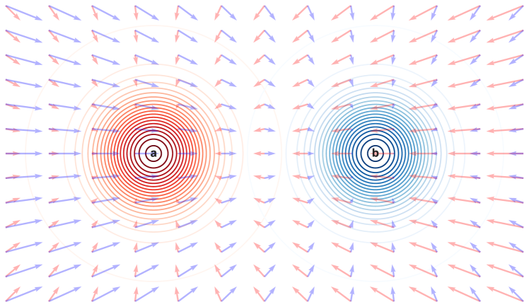
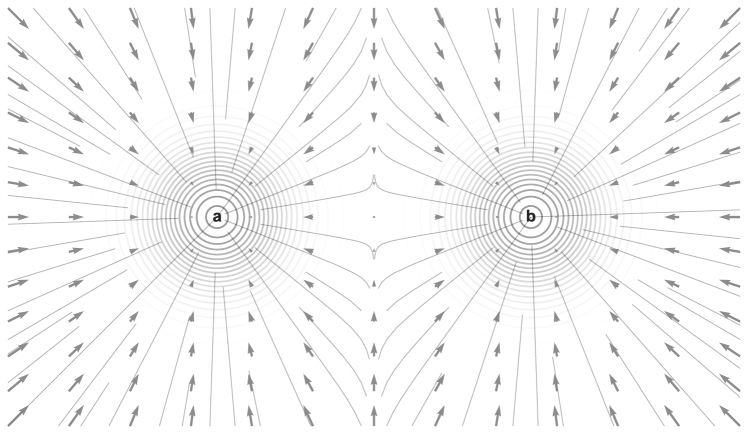
To be intuitively convinced of this, consider the corresponding question about gasses illustrated in Figure 3. Suppose we have two overlapping gases, a red gas with density $𝒩(a,{\sigma }^2)$ and velocity $v_t^{\left[a\right]}$, and a blue gas with density $𝒩(b,{\sigma }^2)$ and velocity $v_t^{\left[b\right]}$. We want to know, what is the effective velocity of the combined gas (as if we saw only in grayscale)? We should clearly take a weighted-average of the individual gas velocities, weighted by their respective densities — just as in Equation (47).

Figure 3: Illustration of combining the velocity fields of two gasses. Left: The density and velocity fields of two independent gases (in red and blue). Right: The effective density and velocity field of the combined gas, including streamlines.

We have now solved the main subproblem of this section: we have found one particular vector field $v_t^{\ast }$ which transports $p_t$ to $p_{t-\mathrm{\Delta }t}$, for our two-point distribution $p_0$. It remains to show that this $v_t^{\ast }$ is equivalent to the velocity field of Algorithm 2 ($v_t$ from Equation 38).

To show this, first notice that the individual vector field $v_t^{\left[a\right]}$ can be written as a conditional expectation. Using the definition in Equation (43),

$v_t^{\left[a\right]}\left(x_t\right)$ $=\lambda \underset{x_0\sim {\delta }_a}{𝔼}\left[x_{t-\mathrm{\Delta }t}-x_t\mid x_t\right]$ (48)

$=\lambda \underset{x_0\sim 1/2{\delta }_a+1/2{\delta }_b}{𝔼}\left[x_{t-\mathrm{\Delta }t}-x_t\mid x_0=a,x_t\right].$ (49)

Now the entire vector field $v_t^{\ast }$ can be written as a conditional expectation:

$v_t^{\ast }\left(x_t\right)$ $=v_t^{\left[a\right]}\left(x_t\right)\cdot p\left(x_0=a\mid x_t\right)+v_t^{\left[b\right]}\left(x_t\right)\cdot p\left(x_0=b\mid x_t\right)$ (50)

$=\lambda 𝔼\left[x_{t-\mathrm{\Delta }t}-x_t\mid x_0=a,x_t\right]\cdot p\left(x_0=a\mid x_t\right)$ (51)

$+\lambda 𝔼\left[x_{t-\mathrm{\Delta }t}-x_t\mid x_0=b,x_t\right]\cdot p\left(x_0=b\mid x_t\right)$ (52)

$=\lambda 𝔼\left[x_{t-\mathrm{\Delta }t}-x_t\mid x_t\right]$ (53)

$=v_t\left(x_t\right)$ (from Equation 38)

where all expectations are w.r.t. the distribution $x_0\sim 1/2{\delta }_a+1/2{\delta }_b$. Thus, the combined velocity field $v_t^{\ast }$ is exactly the velocity field $v_t$ given by the updates of Algorithm 2 — so Algorithm 2 is a correct reverse sampler for our two-point mixture distribution.

3.4 Case 3: Arbitrary Distributions

Now that we know how to handle two points, we can generalize this idea to arbitrary distributions of $x_0$. We will not go into details here, because the general proof will be subsumed by the subsequent section.

It turns out that our overall proof strategy for Algorithm 2 can be generalized significantly to other types of diffusions, without much work. This yields the idea of flow matching, which we will see in the following section. Once we develop the machinery of flows, it is actually straightforward to derive DDIM directly from the simple single-point scaling algorithm of Equation (35): see Appendix B.5.

3.4.1 The Probability Flow ODE [Optional]

Finally, we generalize our discrete-time deterministic sampler to an ordinary differential equation (ODE) called the probability flow ODE (Song et al., 2020). The following section builds on our discussion of SDEs as the continuous limit of diffusion in section 2.4. Just as the reverse-time SDEs of section 2.4 offered a flexible continuous-time generalization of discrete stochastic samplers, so we will see that discrete deterministic samplers generalize to ODEs. The ODE formulation offers both a useful theoretical lens through which to view diffusion, as well as practical advantages, like the opportunity to choose from a variety of off-the-shelf and custom ODE solvers to improve sampling (like the popular DPM++ method, as discussed in chapter 5).

Recall the general SDE (26) from section 2.4:

$$dx=f(x,t)dt+g\left(t\right)dw.$$

Song et al. (2020) showed that is possible to convert this SDE into a deterministic equivalent called the probability flow ODE (PF-ODE):

${\displaystyle \frac{dx}{dt}}$ $=\tilde{f}(x,t),\text{where}\tilde{f}(x,t)=f(x,t)-{\displaystyle \frac{1}{2}}g{\left(t\right)}^2{\nabla }_x\log p_t\left(x\right)$ (54)

SDE (26) and ODE (54) are equivalent in the sense that trajectories obtained by solving the PF-ODE have the same marginal distributions as the SDE trajectories at every point in time. However, note that the score appears here again, as it did in the reverse SDE (27); just as for the reverse SDE, we must learn the score to make the ODE (54) practically useful.

Just as DDPM was a (discretized) special-case of the reverse-time SDE (27), so DDIM can be seen as a (discretized) special case of the PF-ODE (54). Recall from section 2.4 that the simple diffusion we have been studying corresponds to the SDE (25) with $f=0$ and $g={\sigma }_q$. The corresponding ODE is

${\displaystyle \frac{dx}{dt}}$ $=-{\displaystyle \frac{1}{2}}{\sigma }_q^2{\nabla }_x\log p_t\left(x\right)$ (55)

$=-{\displaystyle \frac{1}{2t}}𝔼\left[x_0-x_t\mid x_t\right]\text{(by eq.}\text{<a class="ltx\_ref ltx\_font\_bold" href="https://arxiv.org/html/2406.08929v1\#S2.E28" style="font-size:144\%;" title="In Reverse-Time SDE ‣ 2.4 Diffusions as SDEs [Optional] ‣ 2 Stochastic Sampling: DDPM ‣ Preface ‣ Step-by-Step Diffusion: An Elementary Tutorial"><span class="ltx\_text ltx\_ref\_tag">28</span></a>}\text{)}$ (56)

Reversing and discretizing yields

$x_{t-\mathrm{\Delta }t}$ $=x_t+{\displaystyle \frac{\mathrm{\Delta }t}{2t}}𝔼\left[x_0-x_t\mid x_t\right]$

$=x_t+{\displaystyle \frac{1}{2}}\left(𝔼\left[x_{t-\mathrm{\Delta }t}\mid x_t\right]-x_t\right)\text{(by eq.}\text{<a class="ltx\_ref ltx\_font\_bold" href="https://arxiv.org/html/2406.08929v1\#S2.E23" style="font-size:144\%;" title="In Claim 2. ‣ 2.3 Variance Reduction: Predicting 𝑥₀ ‣ 2 Stochastic Sampling: DDPM ‣ Preface ‣ Step-by-Step Diffusion: An Elementary Tutorial"><span class="ltx\_text ltx\_ref\_tag">23</span></a>}\text{).}$

Noting that ${lim}_{\mathrm{\Delta }t\to 0}\left(\frac{{\sigma }_t}{{\sigma }_{t-\mathrm{\Delta }t}+{\sigma }_t}\right)=\frac{1}{2}$, we recover the deterministic (DDIM) sampler (31).

3.5 Discussion: DDPM vs DDIM

The two reverse samplers defined above (DDPM and DDIM) are conceptually significantly different: one is deterministic, and the other stochastic. To review, these samplers use the following strategies:

1. DDPM ideally implements a stochastic map $F_t$, such that the output $F_t\left(x_t\right)$ is, pointwise, a sample from the conditional distribution $p\left(x_{t-\mathrm{\Delta }t}\mid x_t\right)$.

2. DDIM ideally implements a deterministic map $F_t$, such that the output $F_t\left(x_t\right)$ is marginally distributed as $p_{t-\mathrm{\Delta }t}$. That is, $F_t\mathrm{♯}{p}_t=p_{t-\mathrm{\Delta }t}$.

Although they both happen to take steps in the same direction (given the same input $x_t$), the two algorithms end up evolving very differently. To see this, let’s consider how each sampler ideally behaves, when started from the same initial point $x_1$ and iterated to completion.

DDPM will ideally produce a sample from $p\left(x_0\mid x_1\right)$. If the forward process mixes sufficiently (i.e. for large ${\sigma }_q$ in our setup), then the final point $x_1$ will be nearly independent from the initial point. Thus $p\left(x_0\mid x_1\right)\approx p\left(x_0\right)$, so the distribution output by the ideal DDPM will not depend at all on the starting point $x_1$. In contrast, DDIM is deterministic, so it will always produce a fixed value for a given $x_1$, and thus will depend very strongly on $x_1$.

The picture to have in mind is, DDIM defines a deterministic map ${ℝ}^d\to {ℝ}^d$, taking samples from a Gaussian distribution to our target distribution. At this level, the DDIM map may sound similar to other generative models — after all, GANs and Normalizing Flows also define maps from Gaussian noise to the true distribution. What is special about the DDIM map is, it is not allowed to be arbitrary: the target distribution $p^{\ast }$ exactly determines the ideal DDIM map (which we train models to emulate). This map is “nice”; for example we expect it to be smooth if our target distribution is smooth. GANs, in contrast, are free to learn any arbitrary mapping between noise and images. This feature of diffusion models may make the learning problem easier in some cases (since it is supervised), or harder in other cases (since there may be easier-to-learn maps which other methods could find).

3.6 Remarks on Generalization

In this tutorial, we have not discussed the learning-theoretic aspects of diffusion models: How do we learn properties of the underlying distribution, given only finite samples and bounded compute? These are fundamental aspects of learning, but are not yet fully understood for diffusion models; it is an active area of research.

To appreciate the subtlety here, suppose we learn a diffusion model using the classic strategy of Empirical Risk Minimization (ERM): we sample a finite train set from the underlying distribution, and optimize all regression functions w.r.t. this empirical distribution. The problem is, we should not perfectly minimize the empirical risk, because this would yield a diffusion model which only reproduces the train samples.

In general learning the diffusion model must be regularized, implicitly or explicitly, to prevent overfitting and memorization of the training data. When we train deep neural networks for use in diffusion models, this regularization often occurs implicitly: factors such as finite model size and optimization randomness prevent the trained model from perfectly memorizing its train set. We will revisit these factors (as sources of error) in Section 5.

This issue of memorizing training data has been seen “in the wild” in diffusion models trained on small image datasets, and it has been observed that memorization reduces as the training set size increases (Somepalli et al., 2023; Gu et al., 2023). Additionally, memorization as been noted as a potential security and copyright issue for neural networks as in Carlini et al. (2023) where the authors found they can recover training data from stable diffusion with the right prompts.

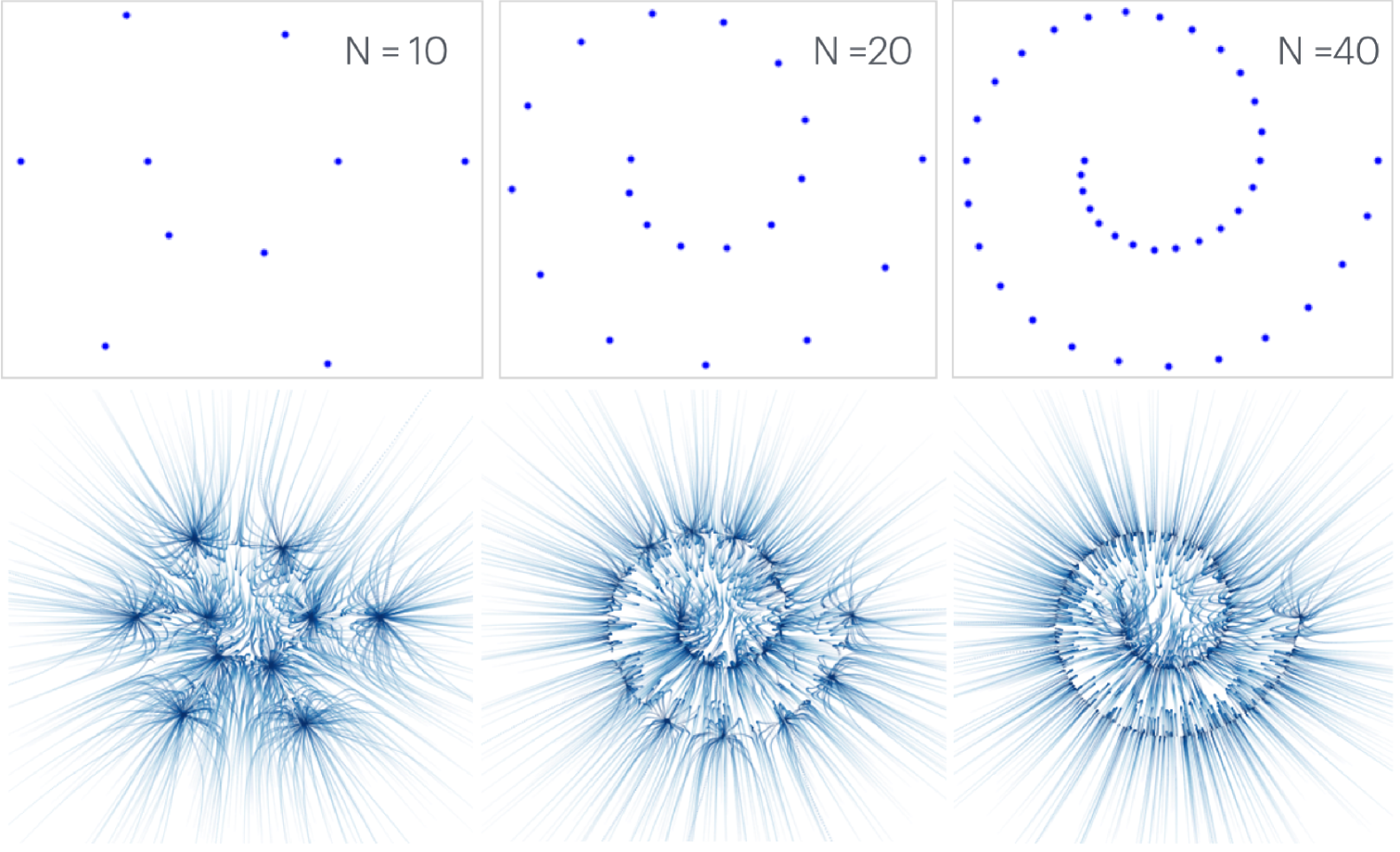
Figure 4 demonstrates the effect of training set size, and shows the DDIM trajectories for a diffusion model trained using a 3 layer ReLU network. We see that the diffusion model on $N=10$ samples “memorizes” its train set: its trajectories all collapse to one of the train points, instead of producing the underlying spiral distribution. As we add more samples, the model starts to generalize: the trajectories converge to the underlying spiral manifold. The trajectories also start to become more perpendicular the underlying manifold, suggesting that the low dimensional structure is being learned. We also note that in the $N=10$ case where the diffusion model fails, it is not at all obvious a human would be able to identify the “correct” pattern from these samples, so generalization may be too much to expect.

Figure 4: The DDIM trajectories (shaded by timestep $t$) for a spiral dataset. We compare the trajectories with $10,20$, and $40$ training samples. Note that as we add more training points (moving left to right) the diffusion algorithm begins to learn the underlying spiral and the trajectories look more perpendicular to the underlying manifold. The network used here is a 3 layer ReLU network with 128 neurons per layer.

4 Flow Matching

Running a flow which generates a spiral distribution (bottom) from an annular distribution (top).

We now introduce the framework of flow matching (Lipman et al., 2023; Albergo et al., 2023; Liu et al., 2022). Flow matching can be thought of as a generalization of DDIM, which allows for more flexibility in designing generative models— including for example the rectified flows (sometimes called linear flows) used by Stable Diffusion 3 (Liu et al., 2022; Esser et al., 2024).

We have actually already seen the main ideas behind flow matching, in our analysis of DDIM in Section 3. At a high level, here is how we constructed a generative model in Section 3:

1. First, we defined how to generate a single point. Specifically, we constructed vector fields ${\left\{v_t^{\left[a\right]}\right\}}_t$ which, when applied for all time steps, transported a standard Gaussian distribution to an arbitrary delta distribution ${\delta }_a$.

2. Second, we determined how to combine two vector fields into a single effective vector field. This lets us construct a transport from the standard Gaussian to two points (or, more generally, to a distribution over points — our target distribution).

Neither of these steps particularly require the Gaussian base distribution, or the Gaussian forward process (Equation 1). The second step of combining vector fields remains identical for any two arbitrary vector fields, for example.

So let’s drop all the Gaussian assumptions. Instead, we will begin by thinking at a basic level about how to map between any two points $x_0$ and $x_1$. Then, we see what happens when the two points are sampled from arbitrary distributions $p$ (data) and $q$ (base), respectively. We will see that this point of view encompasses DDIM as a special case, but that it is significantly more general.

4.1 Flows

Let us first define the central notion of a flow. A flow is simply a collection of time-indexed vector fields $v={\left\{v_t\right\}}_{t\in [0,1]}$. We should think of this as the velocity-field $v_t$ of a gas at each time $t$, as we did earlier in Section 3.2. Any flow defines a trajectory taking initial points $x_1$ to final points $x_0$, by transporting the initial point along the velocity fields $\left\{v_t\right\}$.

Formally, for flow $v$ and initial point $x_1$, consider the ODE] The corresponding discrete-time analog is the iteration: $x_{t-\mathrm{\Delta }t}\leftarrow x_t+v_t(x_t)\mathrm{\Delta }t$, starting at $t=1$ with initial point $x_1$.

${\displaystyle \frac{d{x}_t}{dt}}$ $=-v_t\left(x_t\right),$ (57)

with initial condition $x_1$ at time $t=1$. We write

$x_t:=\mathrm{RunFlow}(v,x_1,t)$ (58)

to denote the solution to the flow ODE (Equation 57) at time $t$, terminating at final point $x_0$. That is, RunFlow is the result of transporting point $x_1$ along the flow $v$ up to time $t$.

Just as flows define maps between initial and final points, they also define transports between entire distributions, by “pushing forward” points from the source distribution along their trajectories. If $p_1$ is a distribution on initial points, then applying the flow $v$ yields the distribution on final points

$$p_0={\left\{\mathrm{RunFlow}\left(v,x_1,t=0\right)\right\}}_{x_1\sim p_1}.$$ (59)

We denote this process as $p_1\stackrel{𝑣}{\hookrightarrow }{p}_0$ meaning the flow $v$ transports initial distribution $p_1$ to final distribution $p_0$.

The ultimate goal of flow matching is to somehow learn a flow $v^{\ast }$ which transports $q\stackrel{v^{\ast }}{\hookrightarrow }p$, where $p$ is the target distribution and $q$ is some easy-to-sample base distribution (such as a Gaussian). If we had this $v^{\ast }$, we could generate samples from our target $p$ by first sampling $x_1\sim q$, then running our flow with initial point $x_1$ and outputting the resulting final point $x_0$. The DDIM algorithm of Section 3 was actually a special case of this, for a very particular choice of flow $v^{\ast }$. Now, how do we construct such flows in general?

4.2 Pointwise Flows

Our basic building-block will be a pointwise flow which just transports a single point $x_1$ to a point $x_0$. Intuitively, given an arbitrary path ${\left\{x_t\right\}}_{t\in [0,1]}$ that connects $x_1$ to $x_0$, a pointwise flow describes this trajectory by giving its velocity $v_t\left(x_t\right)$ at each point $x_t$ along it (see Figure 4.2). Formally, a pointwise flow between ${\mathrm{x}}_1$ and ${\mathrm{x}}_0$ is any flow ${\left\{v_t\right\}}_t$ that satisfies Equation 57 with boundary conditions $x_1$ and $x_0$ at times $t=1,0$ respectively. We denote such flows as $v^{[x_1,x_0]}$. Pointwise flows are not unique: there are many different choices of path between $x_0$ and $x_1$.

A pointwise flow $v_t^{[x_1,x_0]}$ transporting $x_1$ to $x_0$.

4.3 Marginal Flows

Suppose that for all pairs of points $(x_1,x_0)$, we can construct an explicit pointwise flow $v^{[x_1,x_0]}$ that transports a source point $x_1$ to target point $x_0$. For example, we could let $x_t$ travel along a straight line from $x_1$ to $x_0$, or along any other explicit path. Recall in our gas analogy, this corresponds to an individual particle that moves between $x_1$ and $x_0$. Now, let us try to set up a collection of individual particles, such that at $t=1$ the particles are distributed according to $q$, and at $t=0$ they are distributed according to $p$. This is actually easy to do: We can pick any coupling ${\mathrm{\Pi }}_{q,p}$ between $q$ and $p$, and consider particles corresponding to the pointwise flows ${\left\{v^{[x_1,x_0]}\right\}}_{(x_1,x_0)\sim {\mathrm{\Pi }}_{q,p}}$. This gives us a distribution over pointwise flows (i.e. a collection of particle trajectories) with the desired behavior in aggregate.

We would like to combine all of these pointwise flows somehow, to get a single flow $v^{\ast }$ that implements the same transport between distributions. Our previous discussion in Section 3 tells us how to do this: to determine the effective velocity $v_t^{\ast }\left(x_t\right)$, we should take a weighted-average of all individual particle velocities $v_t^{[x_1,x_0]}$, weighted by the probability that a particle at $x_t$ was generated by the pointwise flow $v^{[x_1,x_0]}$. The final result is

$v_t^{\ast }\left(x_t\right)$ $:=\underset{x_0,x_1\mid x_t}{𝔼}\left[v_t^{[x_1,x_0]}\left(x_t\right)\mid x_t\right]$ (62)

where the expectation is w.r.t. the joint distribution of $(x_1,x_0,x_t)$ induced by sampling $(x_1,x_0)\sim {\mathrm{\Pi }}_{q,p}$ and letting $x_t\leftarrow \mathrm{RunFlow}(v^{[x_1,x_0]},x_1,t)$.

At this point, we have a “solution” to our generative modeling problem in principle, but some important questions remain to make it useful in practice:

• Which pointwise flow $v^{[x_1,x_0]}$ and coupling ${\mathrm{\Pi }}_{q,p}$ should we chose?

• How do we compute the marginal flow $v^{\ast }$? We cannot compute it from Equation (62) directly, because this would require sampling from $p\left(x_0\mid x_t\right)$ for a given point $x_t$, which may be complicated in general.

We answer these in the next sections.

4.4 A Simple Choice of Pointwise Flow

Figure 5: A marginal flow with linear pointwise flows, base distribution $q$ uniform over an annulus, and target distribution $p$ equal to a Dirac-delta at $x_0$. (This can also be thought of as the average over $x_1$ of the pointwise linear flows from $x_1\sim q$ to a fixed $x_0$). Gray arrows depict the flow field at different times $t$. The leftmost $(t=1)$ plot shows samples from the base distribution $q$. Subsequent plots show these samples transported by the flow at intermediate times $t$, The final $(t=0)$ plot shows all points collapsed to the target $x_0$. This particular $x_0$ happens to be one point on the spiral distribution of Figure 4.

We need an explicit choices of: pointwise flow, base distribution $q$, and coupling ${\mathrm{\Pi }}_{q,p}$. There are many simple choices which would work.

The base distribution $q$ can be essentially any easy-to-sample distribution. Gaussians are a popular choice but certainly not the only one— Figure 4 uses an annular base distribution, for example. As for the coupling ${\mathrm{\Pi }}_{q,p}$ between the base and target distribution, the simplest choice is the independent coupling, i.e. sampling from $p$ and $q$ independently.

For a pointwise flow, arguably the simplest construction is a linear pointwise flow:

$v_t^{[x_1,x_0]}\left(x_t\right)$ $=x_0-x_1,$ (63)

$⟹\mathrm{RunFlow}(v^{[x_1,x_0]},x_1,t)$ $=t{x}_1+\left(1-t\right)x_0$ (64)

which simply linearly interpolates between $x_1$ and $x_0$ (and corresponds to the choice made in Liu et al. (2022)). In Figure 5 we visualize a marginal flow composed of linear pointwise flows, the same annular base distribution $q$ of Figure 4, and target distribution equal to a point-mass ($p={\delta }_{x_0}$).

4.5 Flow Matching

Now, the only remaining problem is that naively evaluating $v^{\ast }$ using Equation (62) requires sampling from $p\left(x_0\mid x_t\right)$ for a given $x_t$. If we knew how do this for $t=1$, we would have already solved the generative modeling problem!

Fortunately, we can take advantage of the same trick from DDPM: it is enough for us to be able to sample from the joint distribution $(x_0,x_t)$, and then solve a regression problem. Similar to DDPM, the conditional expectation function in Equation (62) can be written as a regressor:

$v_t^{\ast }\left(x_t\right)$ $:=\underset{x_0,x_1\mid x_t}{𝔼}\left[v_t^{[x_1,x_0]}\left(x_t\right)\mid x_t\right]$ (65)

$⟹v_t^{\ast }$ $=\underset{f:{ℝ}^d\to {ℝ}^d}{argmin}\underset{(x_0,x_1,x_t)}{𝔼}{\Vert f\left(x_t\right)-v_t^{[x_1,x_0]}\left(x_t\right)\Vert }_2^2,$ (66)

(by using the generic fact that ${argmin}_f𝔼{\Vert f\left(x\right)-y\Vert }^2=𝔼\left[y\mid x\right]$).

In words, Equation (66) says that to compute the loss of a model $f_{\theta }$ for a fixed time $t$, we should:

1. Sample source and target points $(x_1,x_0)$ from their joint distribution.

2. Compute the point $x_t$ deterministically, by running the pointwise flow $v^{[x_1,x_0]}$ starting from point $x_1$ up to time $t$.

3. Evaluate the model’s prediction at $x_t$, as $f_{\theta }\left(x_t\right)$. Evaluate the deterministic vector $v_t^{[x_1,x_0]}\left(x_t\right)$. Then compute L2 loss between these two quantities.

To sample from the trained model (our estimate of $v_t^{\ast }$), we first sample a source point $x_1\sim q$, then transport it along the learnt flow to a target sample $x_0$. Pseudocode listings 4 and 5 give the explicit procedures for training and sampling from flow-based models (including the special case of linear flows for concreteness; matching Algorithm 1 in Liu et al. (2022).).

Summary

To summarize, here is how to learn a flow-matching generative model for target distribution $p$.

The Ingredients.

We first choose:

1. A source distribution $q$, from which we can efficiently sample (e.g. a standard Gaussian).

2. A coupling ${\mathrm{\Pi }}_{q,p}$ between $q$ and $p$, which specifies a way to jointly sample a pair of source and target points $(x_1,x_0)$ with marginals $q$ and $p$ respectively. A standard choice is the independent coupling, i.e. sample $x_1\sim q$ and $x_0\sim p$ independently.

3. For all pairs of points $(x_1,x_0)$, an explicit pointwise flow $v^{[x_1,x_0]}$ which transports $x_1$ to $x_0$. We must be able to efficiently compute the vector field $v_t^{[x_1,x_0]}$ at all points.

These ingredients determine, in theory, a marginal vector field $v^{\ast }$ which transports $q$ to $p$:

$v_t^{\ast }\left(x_t\right)$ $:=\underset{x_0,x_1\mid x_t}{𝔼}\left[v_t^{[x_1,x_0]}\left(x_t\right)\mid x_t\right]$ (67)

where the expectation is w.r.t. the joint distribution:

$(x_1,x_0)$ $\sim {\mathrm{\Pi }}_{q,p}$

$x_t$ $:=\mathrm{RunFlow}(v^{[x_1,x_0]},x_1,t).$

Training.

Train a neural network $f_{\theta }$ by backpropogating the stochastic loss function computed by Pseudocode 4. The optimal function for this expected loss is: $f_{\theta }(x_t,t)=v_t^{\ast }\left(x_t\right)$.

Sampling.

Run Pseudocode 5 to generate a sample $x_0$ from (approimately) the target distribution $p$.

Input: Neural network $f_{\theta }$

Data: Sample-access to coupling ${\mathrm{\Pi }}_{q,p}$; Pointwise flows $\left\{v_t^{[x_1,x_0]}\right\}$ for all $x_1,x_0$.

Output: Stochastic loss $L$

1 $(x_1,x_0)\leftarrow \mathrm{Sample}\left({\mathrm{\Pi }}_{q,p}\right)$

2 $t\leftarrow \text{Unif}[0,1]$

3 $x_t\leftarrow red\underset{t{x}_1+\left(1-t\right)x_0}{\underbrace{black\mathrm{RunFlow}(v^{[x_1,x_0]},x_1,t)}}$

4 $L\leftarrow {\Vert f_{\theta }(x_t,t)-red\underset{\left(x_0-x_1\right)}{\underbrace{black{v}_t^{[x_1,x_0]}\left(x_t\right)}}\Vert }_2^2$

return $L$

Pseudocode 4 Flow-matching train loss, generic pointwise flow [or linear flow]

Input: Trained network $f_{\theta }$

Data: Sample-access to base distribution $q$; step-size $\mathrm{\Delta }t$.

Output: Sample from target distribution $p$.

1 $x_1\leftarrow \mathrm{Sample}\left(q\right)$

2 for $t=1,(1-\mathrm{\Delta }t),(1-2\mathrm{\Delta }t),\mathrm{\dots },\mathrm{\Delta }t$ do

3 $x_{t-\mathrm{\Delta }t}\leftarrow x_t+f_{\theta }(x_t,t)\mathrm{\Delta }t$

4

5 end for

return $x_0$

Pseudocode 5 Flow-matching sampling

4.6 DDIM as Flow Matching [Optional]

The DDIM algorithm of Section 3 can be seen as a special case of flow matching, for a particular choice of pointwise flows and coupling. We describe the exact correspondence here, which will allow us to notice an interesting relation between DDIM and linear flows.

We claim DDIM is equivalent to flow-matching with the following parameters:

1. Pointwise Flows: Either of the two equivalent pointwise flows:

   $$v_t^{[x_1,x_0]}\left(x_t\right):=\frac{1}{2t}\left(x_t-x_0\right)$$ (68)

   or

   $$v_t^{[x_1,x_0]}\left(x_t\right):=\frac{1}{2\sqrt{t}}\left(x_0-x_1\right),$$ (69)

   which both generate the trajectory:

   $$x_t=x_0+\left(x_1-x_0\right)\sqrt{t}.$$ (70)

2. Coupling: The “diffusion coupling” – that is, the joint distribution on $(x_0,x_1)$ generated by

   $$x_0\sim p;x_1\leftarrow x_0+𝒩(0,{\sigma }_q^2).$$ (71)

This claim is straightforward to prove (see Appendix B.5), but the implication is somewhat surprising: we can recover the DDIM trajectories (which are not straight in general) as a combination of the straight pointwise trajectories in Equation (70). In fact, the DDIM trajectories are exactly equivalent to flow-matching trajectories for the above linear flows, with a different scaling of time ($\sqrt{t}$ vs. $t$). [nobreak]

Claim 4 (DDIM as Linear Flow; Informal).

The DDIM sampler (Algorithm 2) is equivalent, up to time-reparameterization, to the marginal flow produced by linear pointwise flows (Equation 63) with the diffusion coupling (Equation 71).

A formal statement of this claim is provided in Appendix B.7.

4.7 Additional Remarks and References [Optional]

[1cm] The trajectories of individual samples $x_1\sim q$ for the flow in Figure 4.

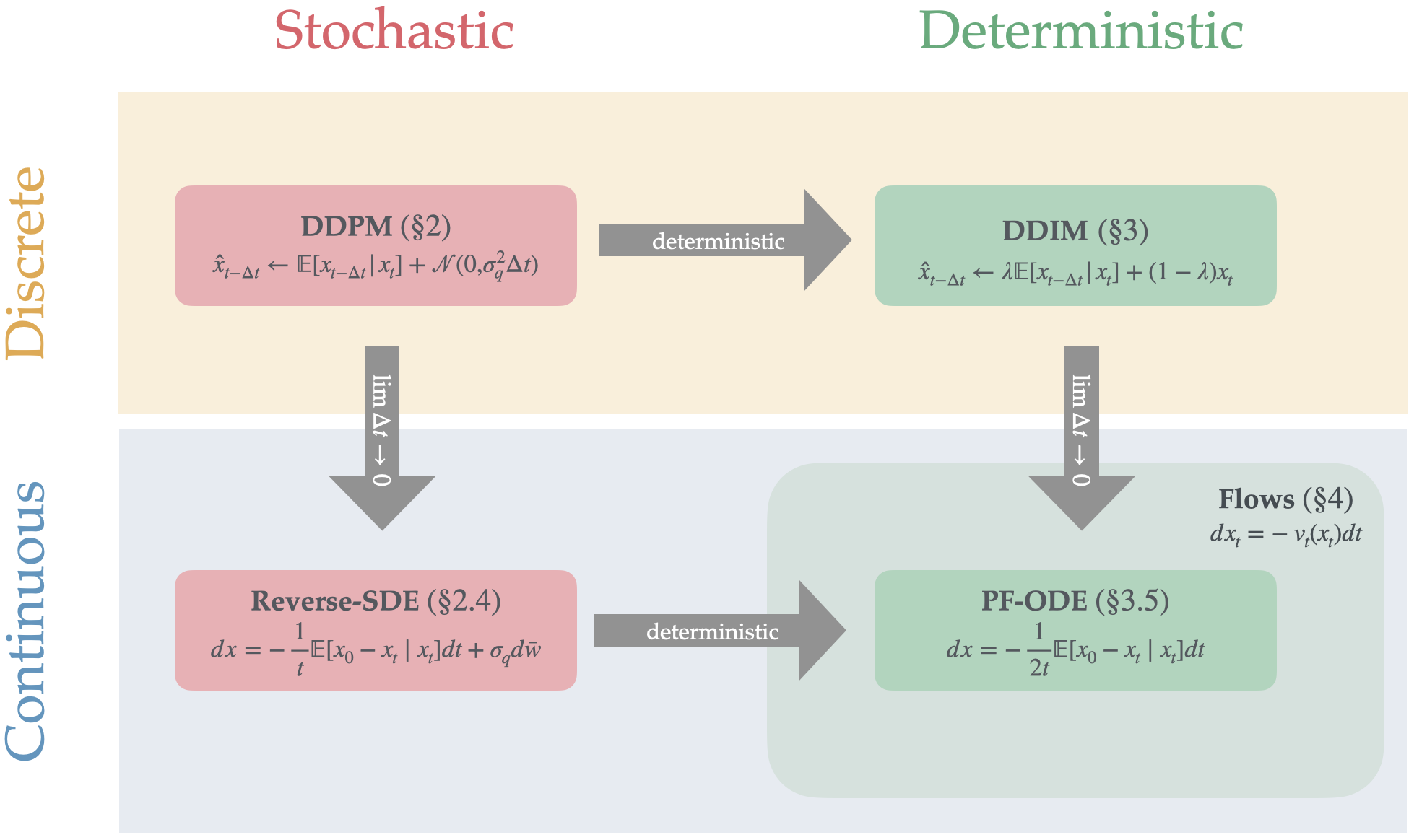
• See Figure 6 for a diagram of the different methods described in this tutorial, and their relations.

• We highly recommend the flow-matching tutorial of Fjelde et al. (2024), which includes helpful visualizations of flows, and uses notation more consistent with the current literature.

• As a curiosity, note that we never had to define an explicit “forward process” for flow-matching, as we did for Gaussian diffusion. Rather, it was enough to define the appropriate “reverse processes” (via flows).

• What we called pointwise flows are also called two-sided conditional flows in the literature, and was developed in Albergo and Vanden-Eijnden (2022); Pooladian et al. (2023); Liu et al. (2022); Tong et al. (2023).

• Albergo et al. (2023) define the framework of stochastic interpolants, which can be thought of as considering stochastic pointwise flows, instead of only deterministic ones. Their framework strictly generalizes both DDPM and DDIM.

• See Stark et al. (2024) for an interesting example of non-standard flows. They derive a generative model for discrete spaces by embedding into a continuous space (the probability simplex), then constructing a special flow on these simplices.

5 Diffusion in Practice

To conclude, we mention some aspects of diffusion which are important in practice, but were not covered in this tutorial.

Samplers in Practice.

Our DDPM and DDIM samplers (algorithms 2 and 3) correspond to the samplers presented in Ho et al. (2020) and Song et al. (2021), respectively, but with different choice of schedule and parametrization (see footnote 13). DDPM and DDIM were some of the earliest samplers to be used in practice, but since then there has been significant progress in samplers for fewer-step generation (which is crucial since each step requires a typically-expensive model forward-pass). In sections 2.4 and 3.4.1, we showed that DDPM and DDIM can be seen as discretizations of the reverse SDE and Probability Flow ODE, respectively. The SDE and ODE perspectives automatically lead to many samplers corresponding to different black-box SDE and ODE numerical solvers (such as Euler, Heun, and Runge-Kutta). It is also possible to take advantage of the specific structure of the diffusion ODE, to improve upon black-box solvers (Lu et al., 2022a, b; Zhang and Chen, 2023).

Noise Schedules.

The noise schedule typically refers to ${\sigma }_t$, which determines the amount of noise added at time $t$ of the diffusion process. The simple diffusion (1) has $p\left(x_t\right)\sim 𝒩(x_0,{\sigma }_t^2)$ with ${\sigma }_t\propto \sqrt{t}$. Notice that the variance of $x_t$ increases at every timestep.

In practice, schedules with controlled variance are often preferred. One of the most popular schedules, introduced in Ho et al. (2020), uses a time-dependent variance and scaling such that the variance of $x_t$ remains bounded. Their discrete update is

$x_t$ $=\sqrt{1-\beta \left(t\right)}{x}_{t-1}+\sqrt{\beta \left(t\right)}{\epsilon }_t;{\epsilon }_t\sim 𝒩(0,1),$ (72)

where is chosen so that $x_t$ is (very close to) clean data at $t=1$ and pure noise at $t=T$.

The general SDE (26) introduced in 2.4 offers additional flexibility. Our simple diffusion (1) has $f=0$, $g={\sigma }_q$, while the diffusion (72) of Ho et al. (2020) has $f=-\frac{1}{2}\beta \left(t\right)$, $g=\sqrt{\beta \left(t\right)}$. Karras et al. (2022) reparametrize the SDE in terms of an overall scaling $s\left(t\right)$ and variance $\sigma \left(t\right)$ of $x_t$, as a more interpretable way to think about diffusion designs, and suggest a schedule with $s\left(t\right)=1$, $\sigma \left(t\right)=t$ (which corresponds to $f=0$, $g=\sqrt{2t}$). Generally, the choice of $f,g$, or equivalently $s,\sigma$, offers a convenient way to explore the design-space of possible schedules.

Likelihood Interpretations and VAEs.

One popular and useful interpretation of diffusion models is the Variational Auto Encoder (VAE) perspective. Briefly, diffusion models can be viewed as a special case of a deep hierarchical VAE, where each diffusion timestep corresponds to one “layer” of the VAE decoder. The corresponding VAE encoder is given by the forward diffusion process, which produces the sequence of noisy $\left\{x_t\right\}$ as the “latents” for input $x$. Notably, the VAE encoder here is not learnt, unlike usual VAEs. Because of the Markovian structure of the latents, each layer of the VAE decoder can be trained in isolation, without forward/backward passing through all previous layers; this helps with the notorious training instability of deep VAEs. We recommend the tutorials of Turner (2021) and Luo (2022) for more details on the VAE perspective.

One advantage of the VAE interpretation is, it gives us an estimate of the data likelihood under our generative model, by using the standard Evidence-Based-Lower-Bound (ELBO) for VAEs. This allows us to train diffusion models directly using a maximum-likelihood objective. It turns out that the ELBO for the diffusion VAE reduces to exactly the L2 regression loss that we presented, but with a particular time-weighting that weights the regression loss differently at different time-steps $t$. For example, regression errors at large times $t$ (i.e. at high noise levels) may need to be weighted differently from errors at small times, in order for the overall loss to properly reflect a likelihood. The best choice of time-weighting in practice, however, is still up for debate: the “principled” choice informed by the VAE interpretation does not always produce the best generated samples. See Kingma and Gao (2023) for a good discussion of different weightings and their effect.

Parametrization: $x_0$ / $\epsilon$ / v -prediction.

Another important practical choice is which of several closely-related quantities – partially-denoised data, fully-denoised data, or the noise itself – we ask the network to predict. Recall that in DDPM Training (Algorithm 1), we asked the network $f_{\theta }$ to learn to predict $𝔼\left[x_{t-\mathrm{\Delta }t}|x_t\right]$ by minimizing ${\Vert f_{\theta }(x_t,t)-x_{t-\mathrm{\Delta }t}\Vert }_2^2$. However, other parametrizations are possible. For example, recalling that $𝔼\left[x_{t-\mathrm{\Delta }t}-x_t|x_t\right]\stackrel{\text{eq.}\text{<a class="ltx\_ref ltx\_font\_italic" href="https://arxiv.org/html/2406.08929v1\#S2.E23" style="font-size:144\%;" title="In Claim 2. ‣ 2.3 Variance Reduction: Predicting 𝑥₀ ‣ 2 Stochastic Sampling: DDPM ‣ Preface ‣ Step-by-Step Diffusion: An Elementary Tutorial"><span class="ltx\_text ltx\_ref\_tag">23</span></a>}}{=}\frac{\mathrm{\Delta }t}{t}𝔼\left[x_0-x_t|x_t\right]$, we see that that

$\underset{𝜃}{\min }$ ${\Vert f_{\theta }(x_t,t)-x_0\Vert }_2^2⟹f_{\theta }^{\star }(x_t,t)=𝔼\left[x_0|x_t\right]$

is a (nearly) equivalent problem, which is often called ${\mathrm{x}}_0$-prediction. The objectives differ only by a time-weighting factor of $\frac{1}{t}$. Similarly, defining the noise ${\epsilon }_t=\frac{1}{{\sigma }_t}𝔼\left[x_0-x_t|x_t\right]$, we see that we could alternatively ask the the network to predict $𝔼\left[{\epsilon }_t|x_t\right]$: this is usually called $\mathrm{\epsilon }$-prediction. Another parametrization, v-prediction, asks the model to predict $v={\alpha }_t\epsilon -{\sigma }_t{x}_0$ (Salimans and Ho, 2022) – mostly predicting data for high noise-levels and mostly noise for low noise-levels. All the parametrizations differ only by time-weightings (see Appendix B.10 for more details).

Although the different time-weightings do not affect the optimal solution, they do impact training as discussed above. Furthermore, even if the time-weightings are adjusted to yield equivalent problems in principle, the different parametrizations may behave differently in practice, since learning is not perfect and certain objectives may be more robust to error. For example, $x_0$-prediction combined with a schedule that places a lot of weight on low noise levels may not work well in practice, since for low noise the identity function can achieve a relatively low objective value, but clearly is not what we want.

Sources of Error.

Finally, when using diffusion and flow models in practice, there are a number of sources of error which prevent the learnt generative model from exactly producing the target distribution. These can be roughly segregated into training-time and sampling-time errors.

1. Train-time error: Regression errors in learning the population-optimal regression function. The regression objective is the marginal flow $v_t^{\ast }$ in flow-matching, or the scores $𝔼\left[x_0\mid x_t\right]$ in diffusion models. For each fixed time $t$, this a standard kind of statistical error. It depends on the neural network architecture and size as well as the number of samples, and can be decomposed further into approximation and estimation errors in the usual way (e.g. see Advani et al. (2020, Sec. 4) decomposing a 2-layer network into approximation error and over-fitting error).

2. Sampling-time error: Discretization errors from using finite step-sizes $\mathrm{\Delta }t$. This error is exactly the discretization error of the ODE or SDE solver used in sampling. These errors manifest in different ways: for DDPM, this reflects the error in using a Gaussian approximation of the reverse process (i.e. Fact 1 breaks for large $\sigma$). For DDIM and flow matching, it reflects the error in simulating continuous-time flows in discrete time.

These errors interact and compound in nontrivial ways, which are not yet fully understood. For example, it is not clear exactly how train-time error in the regression estimates translates into distributional error of the entire generative model. (And this question itself is complicated, since it is not always clear what type of distributional divergence we care about in practice). Interestingly, these “errors” can also have a beneficial effect on small train sets, because they act as a kind of regularization which prevents the diffusion model from just memorizing the train samples (as discussed in Section 3.6).

Conclusion

We have now covered the basics of diffusion models and flow matching. This is an active area of research, and there are many interesting aspects and open questions which we did not cover (see Page A for recommended reading). We hope the foundations here equip the reader to understand more advanced topics in diffusion modeling, and perhaps contribute to the research themselves.

Figure 6: Commutative diagram of the different reverse samplers described in this tutorial, and their relations. Each deterministic sampler produces identical marginal distributions as its stochastic counterpart. There are also various ways to construct stochastic versions of flows, which are not pictured here (e.g. Albergo et al. (2023)).

Appendix A Additional Resources

Several other helpful resources for learning diffusion (tutorials, blogs, papers), roughly in order of mathematical background required.

1. Perspectives on diffusion.
   Dieleman (2023). (Webpage.)
   

   Overview of many interpretations of diffusion, and techniques.

2. Tutorial on Diffusion Models for Imaging and Vision.
   Chan (2024). (49 pgs.)
   

   More focus on intuitions and applications.

3. Interpreting and improving diffusion models using the euclidean distance function.
   Permenter and Yuan (2023). (Webpage.)
   

   Distance-field interpretation. See accompanying blog with simple code (Yuan, 2024).

4. On the Mathematics of Diffusion Models.
   McAllester (2023). (4 pgs.)
   

   Short and accessible.

5. Building Diffusion Model’s theory from ground up
   Das (2024). (Webpage.)
   

   ICLR 2024 Blogposts Track. Focus on SDE and score-matching perspective.

6. Denoising Diffusion Models: A Generative Learning Big Bang.
   Song, Meng, and Vahdat (2023a). (Video, 3 hrs.)
   

   CVPR 2023 tutorial, with recording.

7. Diffusion Models From Scratch.
   Duan (2023). (Webpage, 10 parts.)
   

   Fairly complete on topics, includes: DDPM, DDIM, Karras et al. (2022), SDE/ODE solvers. Includes practical remarks and code.

8. Understanding Diffusion Models: A Unified Perspective.
   Luo (2022). (22 pgs.)
   

   Focus on VAE interpretation, with explicit math details.

9. Demystifying Variational Diffusion Models.
   Ribeiro and Glocker (2024). (44 pgs.)
   

   Focus on VAE interpretation, with explicit math details.

10. Diffusion and Score-Based Generative Models.
    Song (2023). (Video, 1.5 hrs.)
    

    Discusses several interpretations, applications, and comparisons to other generative modeling methods.

11. Deep Unsupervised Learning using Nonequilibrium Thermodynamics
    Sohl-Dickstein, Weiss, Maheswaranathan, and Ganguli (2015). (9 pgs + Appendix)
    

    Original paper introducing diffusion models for ML. Includes unified description of discrete diffusion (i.e. diffusion on discrete state spaces).

12. An Introduction to Flow Matching.
    Fjelde, Mathieu, and Dutordoir (2024). (Webpage.)
    

    Insightful figures and animations, with rigorous mathematical exposition.

13. Elucidating the Design Space of Diffusion-Based Generative Models.
    Karras, Aittala, Aila, and Laine (2022). (10 pgs + Appendix.)
    

    Discusses the effect of various design choices such as noise schhedule, parameterization, ODE solver, etc. Presents a generalized framework that captures many choices.

14. Denoising Diffusion Models
    Peyré (2023). (4 pgs.)
    

    Fast-track through the mathematics, for readers already comfortable with Langevin dynamics and SDEs.

15. Generative Modeling by Estimating Gradients of the Data Distribution.
    Song, Sohl-Dickstein, Kingma, Kumar, Ermon, and Poole (2020). (9 pgs + Appendix.)
    

    Presents the connections between SDEs, ODEs, DDIM, and DDPM.

16. Stochastic Interpolants: A Unifying Framework for Flows and Diffusions.
    Albergo, Boffi, and Vanden-Eijnden (2023). (46 pgs + Appendix.)
    

    Presents a general framework that captures many diffusion variants, and learning objectives. For readers comfortable with SDEs

17. Sampling, Diffusions, and Stochastic Localization.
    Montanari (2023). (22 pgs + Appendix.)
    

    Presents diffusion as a special case of “stochastic localization,” a technique used in high-dimensional statistics to establish mixing of Markov chains.

Appendix B Omitted Derivations

B.1 KL Error in Gaussian Approximation of Reverse Process

Here we prove Lemma 1, restated below.

Lemma 2.

Let $p(x)$ be an arbitrary density over $ℝ$, with bounded 1st to 4th order derivatives. Consider the joint distribution $(x_0,x_1)$, where $x_0\sim p$ and $x_1\sim x_0+𝒩(0,{\sigma }^2)$. Then, for any conditioning $z\in ℝ$ we have

$$\mathrm{KL}\left(𝒩({\mu }_z,{\sigma }^2)\right|\left|p_{x_0\mid x_1}(\cdot \mid x_1=z)\right)\le O\left({\sigma }^4\right)$$ (73)

where

$${\mu }_z:=z+{\sigma }^2\nabla \log p\left(z\right).$$ (74)

Proof.

WLOG, we can take $z=0$. We want to estimate the KL:

$KL\left(𝒩(\mu ,{\sigma }^2)\right|\left|p(x_0=\cdot \mid x_1=0)\right)$ (75)

where we will let $\mu$ be arbitrary for now.

Let $q:=𝒩(\mu ,{\sigma }^2)$, and $p(x)=:\exp (F(x))$. We have $x_1\sim p\star 𝒩(0,{\sigma }^2)$. This implies:

$$p\left(x_1=x\right)=\underset{\eta \sim 𝒩(0,{\sigma }^2)}{𝔼}\left[p\left(x+\eta \right)\right].$$ (76)

Let us first expand the logs of the two distributions we are comparing:

$\log p\left(x_0=x\mid x_1=0\right)$ (77)

$=\log p\left(x_1=0|x_0=x\right)+\log p\left(x_0=x\right)-\log p\left(x_1=0\right)$ (78)

$=-\log \left(\sigma \sqrt{2\pi }\right)-0.5x^2{\sigma }^{-2}+\log p\left(x_0=x\right)-\log p\left(x_1=0\right)$ (79)

$=-\log \left(\sigma \sqrt{2\pi }\right)-0.5x^2{\sigma }^{-2}+F\left(x\right)-\log p\left(x_1=0\right)$ (80)

And also:

$\log q\left(x\right)$ $=-\log \left(\sigma \sqrt{2\pi }\right)-0.5{\left(x-\mu \right)}^2{\sigma }^{-2}$ (82)

Now we can expand the KL:

$KL\left(q\right|\left|p(x_0=\cdot \mid x_1=0)\right)$ (83)

$=\underset{x\sim q}{𝔼}\left[\log q\left(x\right)-\log p\left(x_0=x\mid x_1=0\right)\right]$ (84)

$=\underset{x\sim q}{𝔼}\left[-\log \left(\sigma \sqrt{2\pi }\right)-0.5{\left(x-\mu \right)}^2{\sigma }^{-2}-\left(-\log \left(\sigma \sqrt{2\pi }\right)-0.5x^2{\sigma }^{-2}+F\left(x\right)-\log p\left(x_1=0\right)\right)\right]$ (85)

$=\underset{x\sim q}{𝔼}[-0.5{(x-\mu )}^2{\sigma }^{-2}+0.5x^2{\sigma }^{-2}-F\left(x\right)+\log p(x_1=0))]$ (86)

$=\underset{\eta \sim 𝒩(0,{\sigma }^2);x=\mu +\eta }{𝔼}[-0.5{\eta }^2{\sigma }^{-2}+0.5x^2{\sigma }^{-2}-F\left(x\right)+\log p(x_1=0))]$ (work)

$=-0.5𝔼\left[{\eta }^2\right]{\sigma }^{-2}+0.5𝔼\left[x^2\right]{\sigma }^{-2}-𝔼\left[F\left(x\right)\right]+\log p(x_1=0))]$ (87)

$=-0.5{\sigma }^2{\sigma }^{-2}+0.5({\sigma }^2+{\mu }^2){\sigma }^{-2}-𝔼\left[F\left(x\right)\right]+\log p(x_1=0))]$ (88)

$=0.5{\mu }^2{\sigma }^{-2}+\log p\left(x_1=0\right)-\underset{x\sim q}{𝔼}\left[F\left(x\right)\right]$ (89)

$\approx 0.5{\mu }^2{\sigma }^{-2}+\log p\left(x_1=0\right)-\underset{x\sim q}{𝔼}\left[F\left(0\right)+F^{\prime }\left(0\right)x+0.5F^{\prime \prime }\left(0\right)x^2+O\left(x^3\right)+O\left(x^4\right)\right]$ (90)

$=\log p\left(x_1=0\right)+0.5{\mu }^2{\sigma }^{-2}-F\left(0\right)-F^{\prime }\left(0\right)\mu -0.5F^{\prime \prime }\left(0\right)\left({\mu }^2+{\sigma }^2\right)+O\left({\sigma }^2\mu +{\mu }^2+{\sigma }^4\right)$ (91)

We will now estimate the first term, $\log p(x_1=0)$:

$\log p\left(x_1=0\right)$ (92)

$=\log \underset{\eta \sim 𝒩(0,{\sigma }^2)}{𝔼}\left[p\left(\eta \right)\right]$ (93)

$=\log \underset{\eta \sim 𝒩(0,{\sigma }^2)}{𝔼}\left[p\left(0\right)+p^{\prime }\left(0\right)\eta +0.5p^{\prime \prime }\left(0\right){\eta }^2+O\left({\eta }^3\right)+O\left({\eta }^4\right)\right]$ (94)

$=\log \left(p\left(0\right)+0.5p^{\prime \prime }\left(0\right){\sigma }^2+O\left({\sigma }^4\right)\right)$ (95)

$=\log p\left(0\right)+{\displaystyle \frac{0.5p^{\prime \prime }\left(0\right){\sigma }^2+O\left({\sigma }^4\right)}{p\left(0\right)}}+O\left({\sigma }^4\right)$ (Taylor expand $\log (p(0)+\epsilon )$ around $p(0)$)

$=\log p\left(0\right)+0.5{\sigma }^2{\displaystyle \frac{p^{\prime \prime }\left(0\right)}{p\left(0\right)}}+O\left({\sigma }^4\right)$ (96)

To compute the derivatives of $p$, observe that:

$F\left(x\right)$ $=\log p\left(x\right)$ (97)

$⟹F^{\prime }\left(x\right)$ $=p^{\prime }\left(x\right)/p\left(x\right)$ (98)

$⟹F^{\prime \prime }\left(x\right)$ $=p^{\prime \prime }\left(x\right)/p\left(x\right)-{\left(p^{\prime }\left(x\right)/p\left(x\right)\right)}^2$ (99)

$=p^{\prime \prime }\left(x\right)/p\left(x\right)-{\left(F^{\prime }\left(x\right)\right)}^2$ (100)

$⟹p^{\prime \prime }\left(x\right)/p\left(x\right)$ $=F^{\prime \prime }\left(x\right)+{\left(F^{\prime }\left(x\right)\right)}^2$ (101)

Thus, continuing from line (96):

$\log p\left(x_1=0\right)$ $=\log p\left(0\right)+0.5{\sigma }^2{\displaystyle \frac{p^{\prime \prime }\left(0\right)}{p\left(0\right)}}+O\left({\sigma }^4\right)$ (102)

$=F\left(0\right)+0.5{\sigma }^2\left(F^{\prime \prime }\left(0\right)-F^{\prime }{\left(0\right)}^2\right)+O\left({\sigma }^4\right)$ (by Line 101)

We can now plug this estimate of $\log p(x_1=0)$ into Line (91). We omit the argument $(0)$ from $F$ for simplicity:

$KL\left(q\right|\left|p(x_0=\cdot \mid x_1=0)\right)$ (103)

$=\boxed{\log p\left(x_1=0\right)}+0.5{\mu }^2{\sigma }^{-2}-F-F^{\prime }\mu -0.5F^{\prime \prime }\left({\mu }^2+{\sigma }^2\right)+O\left({\mu }^4+{\sigma }^4\right)$ (104)

$=F+0.5{\sigma }^2\left(F^{\prime \prime }+F^{\prime 2}\right)+0.5{\mu }^2{\sigma }^{-2}-F-F^{\prime }\mu -0.5F^{\prime \prime }\left({\mu }^2+{\sigma }^2\right)+O\left({\mu }^4+{\sigma }^4\right)$ (105)

$=+0.5{\sigma }^2{F}^{\prime \prime }+0.5{\sigma }^2{F}^{\prime 2}+0.5{\mu }^2{\sigma }^{-2}-F^{\prime }\mu -0.5F^{\prime \prime }{\mu }^2-0.5F^{\prime \prime }{\sigma }^2+O\left({\mu }^4+{\sigma }^4\right)$ (106)

$=-F^{\prime }\mu +0.5{\mu }^2{\sigma }^{-2}+0.5F^{\prime 2}{\sigma }^2-0.5F^{\prime \prime }{\mu }^2+O\left({\mu }^4+{\sigma }^4\right)$ (107)

Up to this point, $\mu$ was arbitrary. We now set

$${\mu }_{\ast }:=F^{\prime }\left(0\right){\sigma }^2.$$ (108)

And continue:

$KL\left(q\right|\left|p(x_0=\cdot \mid x_1=0)\right)$ (109)

$=-F^{\prime }{\mu }_{\ast }+0.5{\mu }_{\ast }^2{\sigma }^{-2}+0.5F^{\prime 2}{\sigma }^2-0.5F^{\prime \prime }{\mu }_{\ast }^2+O\left({\mu }_{\ast }^4+{\sigma }^4\right)$ (110)

$=-F^{\prime 2}{\sigma }^2+0.5F^{\prime 2}{\sigma }^2+0.5F^{\prime 2}{\sigma }^2+O\left({\sigma }^4\right)$ (111)

$=O\left({\sigma }^4\right)$ (112)

as desired.

∎

Notice that our choice of ${\mu }_{\ast }$ in the above proof was crucial; for example if we had set ${\mu }_{\ast }=0$, the $\mathrm{\Omega }\left({\sigma }^2\right)$ terms in Line (111) would not have cancelled out.

B.2 SDE proof sketches

Here is sketch of the proof of the equivalence of the SDE and Probability Flow ODE, which relies on the equivalence of the SDE to a Fokker-Planck equation. (See Song et al. (2020) for full proof.)

Proof.

$dx$ $=f(x,t)dt+g\left(t\right)dw$

$\iff {\displaystyle \frac{\partial p_t\left(x\right)}{\partial t}}$ $=-{\nabla }_x\left(f{p}_t\right)+{\displaystyle \frac{1}{2}}{g}^2{\nabla }_x^2{p}_t\text{(FP)}$

$=-{\nabla }_x\left(f{p}_t\right)+{\displaystyle \frac{1}{2}}{g}^2{\nabla }_x\left(p_t{\nabla }_x\log p_t\right)$

$=-{\nabla }_x\left\{\left(f-{\displaystyle \frac{1}{2}}{g}^2{\nabla }_x\log p_t\right)p_t\right\}$

$=-{\nabla }_x\left\{\tilde{f}(x,t)p_t\left(x\right)\right\},\tilde{f}(x,t)=f(x,t)-{\displaystyle \frac{1}{2}}g{\left(t\right)}^2{\nabla }_x\log p_t\left(x\right)$

$⟹dx$ $=\tilde{f}(x,t)dt$

∎

The equivalence of the SDE and Fokker-Planck equations follows from Itô’s formula and integration-by-parts. Here is an outline for a simplified case in 1d, where $g$ is constant (see Winkler (2023) for full proof):

Proof.

$dx$ $=f\left(x\right)dt+gdw,dw\sim \sqrt{dt}𝒩(0,1)$

$\text{For any}\varphi \text{:}d\varphi \left(x\right)$ $=(f\left(x\right){\partial }_x\varphi \left(x\right)+{\displaystyle \frac{1}{2}}{g}^2{\partial }_x^2\varphi \left(x\right))dt+g\partial {}_x\varphi (x)dw$ Itô’s formula

$⟹{\displaystyle \frac{d}{dt}}𝔼\left[\varphi \right]$ $=𝔼\left[f{\partial }_x\varphi +{\displaystyle \frac{1}{2}}{g}^2{\partial }_x^2\varphi \right],\left(𝔼\left[dw\right]=0\right)$

${\displaystyle \int \varphi \left(x\right){\partial }_{t}p(x,t)dx}$ $={\displaystyle \int f\left(x\right){\partial }_x\varphi \left(x\right)p(x,t)dx}+{\displaystyle \frac{1}{2}}{g}^2{\displaystyle \int {\partial }_x^2\varphi \left(x\right)p(x,t)dx}$

$=-{\displaystyle \int \varphi \left(x\right){\partial }_x\left(f\left(x\right)p(x,t)\right)dx}+{\displaystyle \frac{1}{2}}{g}^2{\displaystyle \int \varphi \left(x\right){\partial }_x^{2}p(x,t)dx},$ integration-by-parts

${\partial }_{t}p\left(x\right)$ $=-{\partial }_x\left(f\left(x\right)p(x,t)\right)+{\displaystyle \frac{1}{2}}{g}^2{\partial }_x^{2}p\left(x\right),$ Fokker-Planck

∎

B.3 DDIM Point-mass Claim

Here is a version of Claim 3 where $p_0$ is a delta at an arbitrary point $x_0$.

Claim 5.

Suppose the target distribution is a point mass at $x_0\in {ℝ}^d$, i.e. $p_0={\delta }_{x_0}$. Define the function

$G_t\left[x_0\right]\left(x_t\right)=\left({\displaystyle \frac{{\sigma }_{t-\mathrm{\Delta }t}}{{\sigma }_t}}\right)\left(x_t-x_0\right)+x_0.$ (113)

Then we clearly have $G_t[x_0]\mathrm{♯}{p}_t=p_{t-\mathrm{\Delta }t}$, and moreover

$$G_t\left[x_0\right]\left(x_t\right)=x_t+\lambda (𝔼[x_{t-\mathrm{\Delta }t}\mid x_t]-x_t)=:F_t\left(x_t\right).$$ (114)

Thus Algorithm 2 defines a valid reverse sampler for target distribution $p_0={\delta }_{x_0}.$

B.4 Flow Combining Lemma

Here we provide a more formal statement of the marginal flow result stated in Equation (62).

Equation (62) follows from a more general lemma (Lemma 3) which formalizes the “gas combination” analogy of Section 3. The motivation for this lemma is, we need a way of combining flows: of taking several different flows and producing a single “effective flow.” As a warm-up for the lemma, suppose we have $n$ different flows, each with their own initial and final distributions $q_i,p_i$:

$q_1\stackrel{v^{\left(1\right)}}{\hookrightarrow }{p}_1,q_2\stackrel{v^{\left(2\right)}}{\hookrightarrow }{p}_2,\mathrm{\dots },q_n\stackrel{v^{\left(n\right)}}{\hookrightarrow }{p}_n$

We can imagine these as the flow of $n$ different gases, where gas $i$ has initial density $q_i$ and final density $p_i$. Now we want to construct an overall flow $v^{\ast }$ which takes the average initial-density to the average final-density:

$$\underset{i\in \left[n\right]}{𝔼}\left[q_i\right]\stackrel{v^{\ast }}{\hookrightarrow }\underset{i\in \left[n\right]}{𝔼}\left[p_i\right].$$ (115)

To construct $v_t^{\ast }\left(x_t\right)$, we must take an average of the individual vector fields $v^{\left(i\right)}$, weighted by the probability mass the $i$-th flow places on $x_t$, at time $t$. (This is exactly analogous to Figure 3).

This construction is formalized in Lemma 3. There, instead of averaging over just a finite set of flows, we are allowed to average over any distribution over flows. To recover Equation (62), we can apply Lemma 3 to a distribution $\mathrm{\Gamma }$ over $(v,q_v)=(v^{[x_1,x_0]},{\delta }_{x_1})$, that is, pointwise flows and their associated initial delta distributions.

[nobreak]

Lemma 3 (Flow Combining Lemma).

Let $\mathrm{\Gamma }$ be an arbitrary joint distribution over pairs $(v,q_v)$ of flows $v$ and their associated initial distributions $q_v$. Let $v(q_v)$ denote the final distribution when initial distribution $q_v$ is transported by flow $v$, so $q_v\stackrel{𝑣}{\hookrightarrow }v(q_v)$

For fixed $t\in [0,1]$, consider the joint distribution over $(x_1,x_t,w_t)\in {({ℝ}^d)}^3$ generated by:

$(v,q_v)$ $\sim \mathrm{\Gamma }$

$x_1$ $\sim q_v$

$x_t$ $:=\mathrm{RunFlow}(v,x_1,t)$

$w_t$ $:=v_t\left(x_t\right).$

Then, taking all expectations w.r.t. this joint distribution, the flow $v^{\ast }$ defined as

$v_t^{\ast }\left(x_t\right)$ $:=𝔼\left[w_t\mid x_t\right]$ (116)

$=𝔼\left[v_t\left(x_t\right)\mid x_t\right]$ (117)

is known as the marginal flow for $\mathrm{\Gamma }$, and transports:

$𝔼\left[q_v\right]\stackrel{v^{\ast }}{\hookrightarrow }𝔼\left[v\left(q_v\right)\right].$ (118)

B.5 Derivation of DDIM using Flows

Now that we have the machinery of flows in hand, it is fairly easy to derive the DDIM algorithm “from scratch”, by extending our simple scaling algorithm from the single point-mass case.

First, we need to find the pointwise flow. Recall from Claim 5 that for the simple case where the target distribution $p_0$ is a Dirac-delta at $x_0$, the following scaling maps $p_t$ to $p_{t-\mathrm{\Delta }t}$:

$G_t\left[x_0\right]\left(x_t\right)=\left({\displaystyle \frac{{\sigma }_{t-\mathrm{\Delta }t}}{{\sigma }_t}}\right)\left(x_t-x_0\right)+x_0⟹G_t\mathrm{♯}{p}_t=p_{t-\mathrm{\Delta }t}.$

$G_t$ implies the pointwise flow:

$\underset{t\to 0}{lim}\left({\displaystyle \frac{{\sigma }_{t-\mathrm{\Delta }t}}{{\sigma }_t}}\right)$ $=\sqrt{1-{\displaystyle \frac{\mathrm{\Delta }t}{t}}}=\left(1-{\displaystyle \frac{\mathrm{\Delta }t}{2t}}\right)$

$⟹v_t^{[x_1,x_0]}\left(x_t\right)$ $=-\underset{\mathrm{\Delta }t\to 0}{lim}{\displaystyle \frac{G_t\left(x_t\right)-x_t}{\mathrm{\Delta }t}}={\displaystyle \frac{1}{2t}}\left(x_t-x_0\right),$

which agrees with (68).

Now let us compute the marginal flow $v^{\ast }$ generated by the pointwise flow of Equation (68) and the coupling implied by the diffusion forward process. By Equation (67), the marginal flow is:

$v_t^{\ast }\left(x_t\right)$ $=\underset{x_1,x_0\mid x_t}{𝔼}\left[v_t^{[x_1,x_0]}\left(x_t\right)\mid x_t\right]$ By gas-lemma.

$={\displaystyle \frac{1}{2t}}\underset{\begin{array}{c}{x}_0\sim p;x_1\leftarrow x_0+𝒩(0,{\sigma }_q^2)\\ x_t\leftarrow \mathrm{RunFlow}(v_t^{[x_1,x_0]},x_1,t)\end{array}}{𝔼}\left[x_0-x_t\mid x_t\right]$ For our choices of coupling and flow.

$={\displaystyle \frac{1}{2t}}\underset{\begin{array}{c}{x}_0\sim p;x_1\leftarrow x_0+𝒩(0,{\sigma }_q^2)\\ x_t\leftarrow x_1\sqrt{t}+(1-\sqrt{t})x_0\end{array}}{𝔼}\left[x_0-x_t\mid x_t\right]$ Expanding the flow trajectory.

$={\displaystyle \frac{1}{2t}}\underset{\begin{array}{c}{x}_0\sim p\\ x_t\leftarrow \sqrt{t}𝒩(0,{\sigma }_q^2)\end{array}}{𝔼}\left[x_0-x_t\mid x_t\right]$ Plugging in $x_1=x_0+𝒩(0,{\sigma }_q^2).$

This is exactly the differential equation describing the trajectory of DDIM (see Equation 56, which is the continuous-time limit of Equation 31).

B.6 Two Pointwise Flows for DDIM give the same Trajectory

We want to show that pointwise flow 69:

$$v_t^{[x_1,x_0]}\left(x_t\right)=\frac{1}{2\sqrt{t}}\left(x_0-x_1\right)$$ (119)

is equivalent to the DDIM pointwise flow (68):

$$v_t^{[x_1,x_0]}\left(x_t\right)=\frac{1}{2t}\left(x_t-x_0\right)$$ (120)

because both these pointwise flows generate the same trajectory of $x_t$:

$$x_t=x_0+\left(x_1-x_0\right)\sqrt{t}.$$ (121)

To see this, we can solve the ODE determined by (68) via the Separable Equations method:

${\displaystyle \frac{d{x}_t}{dt}}$ $=-{\displaystyle \frac{1}{2t}}\left(x_0-x_t\right)$

$⟹{\displaystyle \frac{\frac{d{x}_t}{dt}}{x_t-x_0}}$ $={\displaystyle \frac{1}{2t}}$

$⟹{\displaystyle \int \frac{1}{x_t-x_0}𝑑x}$ $={\displaystyle \int \frac{1}{2t}𝑑t},\text{since}{\displaystyle \frac{d{x}_t}{dt}}dt=dx$

$⟹\log \left(x_t-x_0\right)$ $=\log \sqrt{t}+c$

$c$ $=\log \left(x_1-x_0\right)\text{(boundary cond.)}$

$⟹\log \left(x_t-x_0\right)$ $=\log \sqrt{t}\left(x_1-x_0\right)$

$⟹x_t-x_0$ $=\sqrt{t}\left(x_1-x_0\right).$

B.7 DDIM vs Time-reparameterized linear flows

Lemma 4 (DDIM vs Linear Flows).

Let $p_0$ be an arbitrary target distribution. Let ${\{x_t\}}_t$ be the joint distribution defined by the DDPM forward process applied to $p_0$, so the marginal distribution of $x_t$ is $p_t=p\star 𝒩(0,t{\sigma }_q^2)$.

Let $x^{\ast }\in {ℝ}^d$ be an arbitrary initial point. Consider the following two deterministic trajectories:

1. The trajectory ${\left\{y_t\right\}}_t$ of the continuous-time DDIM flow, with respect to target distribution $p_0$, when started at initial point $y_1=x^{\ast }$.

   That is, $y_t$ is the solution to the following ODE (Equation 56):

   ${\displaystyle \frac{d{y}_t}{dt}}$ $=-v^{\mathrm{ddim}}\left(y_t\right)$ (122)

   $=-{\displaystyle \frac{1}{2t}}\underset{x_0\mid x_t}{𝔼}\left[x_0-x_t\mid x_t=y_t\right]$ (123)

   with boundary condition $y_1$ at $t=1$.

2. The trajectory ${\left\{z_t\right\}}_t$ produced when initial point $z_1=x^{\ast }$ is transported by the marginal flow constructed from:

   • Linear pointwise flows

   • The DDPM-coupling of Line (71).

   That is, the marginal flow

   $v_t^{\star }\left(x_t\right)$ $=\underset{x_0,x_1|x_t}{𝔼}\left[v^{[x_1,x_0]}\left(x_t\right)|x_t\right]$

   $:=\underset{x_0,x_1|x_t}{𝔼}\left[x_0-x_1|x_t\right]$

   $=\underset{x_0|x_t}{𝔼}\left[x_0-x_t|x_t\right]$ since $𝔼[x_1|x_t]=x_t$ under the DDPM coupling.

Then, we claim these two trajectories are identical with the following time-reparameterization:

$\forall t\in [0,1]:y_t=z_{\sqrt{t}}$ (124)

B.8 Proof Sketch of Claim 2

We will show that, in the forward diffusion setup of Section 1:

$𝔼\left[\left(x_t-x_{t-\mathrm{\Delta }t}\right)\mid x_t\right]={\displaystyle \frac{\mathrm{\Delta }t}{t}}𝔼\left[\left(x_t-x_0\right)\mid x_t\right].$ (125)

Proof sketch.

Recall ${\eta }_t=x_{t+\mathrm{\Delta }t}-x_t$. So by linearity of expectation:

$𝔼\left[\left(x_t-x_0\right)\mid x_t\right]$ (126)

(127)

Now, we claim that for given $x_t$, the conditional distributions $p({\eta }_i\mid x_t)$ are identical for all . To see this, notice that the joint distribution function $p(x_0,x_t,{\eta }_0,{\eta }_{\mathrm{\Delta }t},\mathrm{\dots },{\eta }_{t-\mathrm{\Delta }t})$ is symmetric in the $\{{\eta }_i\}$s, by definition of the forward process, and therefore the conditional distribution function $p({\eta }_0,{\eta }_{\mathrm{\Delta }t},\mathrm{\dots },{\eta }_{t-\mathrm{\Delta }t}\mid x_t)$ is also symmetric in the $\{{\eta }_i\}$s. Therefore, all ${\eta }_i$ have identical conditional expectations:

$$𝔼\left[{\eta }_0\mid x_t\right]=𝔼\left[{\eta }_{\mathrm{\Delta }t}\mid x_t\right]=\mathrm{\cdots }=𝔼\left[{\eta }_{t-\mathrm{\Delta }t}\mid x_t\right]$$ (128)

And since there are $(t/\mathrm{\Delta }t)$ of them,

(129)

Now continuing from Line 127,

$𝔼\left[\left(x_0-x_t\right)\mid x_t\right]$ (130)

$=\left(t/\mathrm{\Delta }t\right)𝔼\left[{\eta }_{t-\mathrm{\Delta }t}\mid x_t\right]$ (131)

$=\left(t/\mathrm{\Delta }t\right)𝔼\left[\left(x_t-x_{t-\mathrm{\Delta }t}\right)\mid x_t\right]$ (132)

as desired. ∎

B.9 Variance-Reduced Algorithms

Here we give the “varianced-reduced” versions of the DDPM training and sampling algorithms, where we train a network $g_{\theta }$ to approximate

$$g_{\theta }(x,t)\approx 𝔼\left[x_0\mid x_t\right]$$ (133)

instead of a network $f_{\theta }$ to approximate

$$f_{\theta }(x,t)\approx 𝔼\left[x_{t-\mathrm{\Delta }t}\mid x_t\right].$$ (134)

Via Claim 2, these two functions are equivalent via the transform:

$$f_{\theta }(x,t)=\left(\mathrm{\Delta }t/t\right)g_{\theta }(x,t)+\left(1-\mathrm{\Delta }t/t\right)x.$$ (135)

Plugging this relation into Pseudocode 2 yields the variance-reduced DDPM sampler of Pseudocode 7.

Input: Neural network $g_{\theta }$; Sample-access to train distribution $p$.

Data: Terminal variance ${\sigma }_q$

Output: Stochastic loss $L$

1 $x_0\leftarrow \text{Sample}\left(p\right)$

2 $t\leftarrow \text{Unif}[0,1]$

3 $x_t\leftarrow x_0+𝒩(0,{\sigma }_q^{2}t)$

4 $L\leftarrow {\Vert g_{\theta }(x_t,t)-x_0\Vert }_2^2$

return $L$

Pseudocode 6 DDPM train loss ($x_0$-prediction)

Input: Trained model $f_{\theta }$.

Data: Terminal variance ${\sigma }_q$; step-size $\mathrm{\Delta }t$.

Output: $x_0$

1 $x_1\leftarrow 𝒩(0,{\sigma }_q^2)$

2 for $t=1,(1-\mathrm{\Delta }t),(1-2\mathrm{\Delta }t),\mathrm{\dots },\mathrm{\Delta }t$ do

3 $\widehat{{\eta }_t}\leftarrow g_{\theta }(x_t,t)-x_t$

4 $x_{t-\mathrm{\Delta }t}\leftarrow x_t+\left(1/t\right)\widehat{{\eta }_t}\mathrm{\Delta }t+𝒩(0,{\sigma }_q^2\mathrm{\Delta }t)$

5

6 end for

return $x_0$

Pseudocode 7 DDPM sampling ($x_0$-prediction)

B.10 Equivalence of and $x_0$- and $\epsilon$-prediction

We will discuss this in our usual simplified setup:

$x_t$ $=x_0+{\sigma }_t{\epsilon }_t,{\sigma }_t={\sigma }_q\sqrt{t},{\epsilon }_t\sim 𝒩(0,1);$

the scaling factors are more complex in the general case (see Luo (2022) for VP diffusion, for example) but the idea is the same. The DDPM training algorithm 1 has objective and optimal value

$\underset{𝜃}{\min }$ ${\Vert f_{\theta }(x_t,t)-x_{t-\mathrm{\Delta }t}\Vert }_2^2,f_{\theta }^{\star }(x_t,t)=𝔼\left[x_{t-\mathrm{\Delta }t}|x_t\right]$

That is, the network $f_{\theta }$ to learn to predict $𝔼\left[x_{t-\mathrm{\Delta }t}|x_t\right]$. However, we could instead require the network to predict other related quantities, as follows. Noting that

$𝔼\left[x_{t-\mathrm{\Delta }t}-x_t|x_t\right]\stackrel{\text{eq.}\text{<a class="ltx\_ref ltx\_font\_italic" href="https://arxiv.org/html/2406.08929v1\#S2.E23" style="font-size:144\%;" title="In Claim 2. ‣ 2.3 Variance Reduction: Predicting 𝑥₀ ‣ 2 Stochastic Sampling: DDPM ‣ Preface ‣ Step-by-Step Diffusion: An Elementary Tutorial"><span class="ltx\_text ltx\_ref\_tag">23</span></a>}}{=}{\displaystyle \frac{\mathrm{\Delta }t}{t}}𝔼\left[x_0-x_t|x_t\right]\equiv {\displaystyle \frac{\mathrm{\Delta }t}{t{\sigma }_t}}𝔼\left[{\epsilon }_t|x_t\right]$

$⟹$ $\parallel E[x_{t-\mathrm{\Delta }t}-x_t|x_t]-x_{t-\mathrm{\Delta }t}{\parallel }_2^2=\parallel {\displaystyle \frac{\mathrm{\Delta }t}{t}}(𝔼\left[x_0\right|x_t]-x_0){\parallel }_2^2=\parallel {\displaystyle \frac{\mathrm{\Delta }t}{t{\sigma }_t}}(𝔼\left[{\epsilon }_t\right|x_t]-{\epsilon }_t){\parallel }_2^2$

we get the following equivalent problems:

$\underset{𝜃}{\min }$ ${\Vert f_{\theta }(x_t,t)-x_0\Vert }_2^2⟹f_{\theta }^{\star }(x_t,t)=𝔼\left[x_0|x_t\right],\text{time-weighting}={\displaystyle \frac{1}{t}}$

$\underset{𝜃}{\min }$ ${\Vert {\displaystyle \frac{\mathrm{\Delta }t}{t{\sigma }_t}}\left(f_{\theta }(x_t,t)-{\epsilon }_t\right)\Vert }_2^2⟹f_{\theta }^{\star }(x_t,t)=𝔼\left[{\epsilon }_t|x_t\right]\text{time-weighting}={\displaystyle \frac{1}{t{\sigma }_t}}.$

References

- Advani et al. [2020] Madhu S Advani, Andrew M Saxe, and Haim Sompolinsky. High-dimensional dynamics of generalization error in neural networks. Neural Networks, 132:428–446, 2020.
- Albergo et al. [2023] Michael S. Albergo, Nicholas M. Boffi, and Eric Vanden-Eijnden. Stochastic interpolants: A unifying framework for flows and diffusions, 2023.
- Albergo and Vanden-Eijnden [2022] Michael Samuel Albergo and Eric Vanden-Eijnden. Building normalizing flows with stochastic interpolants. In The Eleventh International Conference on Learning Representations, 2022.
- Anderson [1982] Brian DO Anderson. Reverse-time diffusion equation models. Stochastic Processes and their Applications, 12(3):313–326, 1982.
- Carlini et al. [2023] Nicolas Carlini, Jamie Hayes, Milad Nasr, Matthew Jagielski, Vikash Sehwag, Florian Tramer, Borja Balle, Daphne Ippolito, and Eric Wallace. Extracting training data from diffusion models. In 32nd USENIX Security Symposium (USENIX Security 23), pages 5253–5270, 2023.
- Chan [2024] Stanley H. Chan. Tutorial on diffusion models for imaging and vision, 2024.
- Chen et al. [2023] Hongrui Chen, Holden Lee, and Jianfeng Lu. Improved analysis of score-based generative modeling: User-friendly bounds under minimal smoothness assumptions. In International Conference on Machine Learning, pages 4735–4763. PMLR, 2023.
- Chen et al. [2022] Sitan Chen, Sinho Chewi, Jerry Li, Yuanzhi Li, Adil Salim, and Anru Zhang. Sampling is as easy as learning the score: theory for diffusion models with minimal data assumptions. In The Eleventh International Conference on Learning Representations, 2022.
- Chen et al. [2024a] Sitan Chen, Sinho Chewi, Holden Lee, Yuanzhi Li, Jianfeng Lu, and Adil Salim. The probability flow ode is provably fast. Advances in Neural Information Processing Systems, 36, 2024a.
- Chen et al. [2024b] Sitan Chen, Vasilis Kontonis, and Kulin Shah. Learning general gaussian mixtures with efficient score matching. arXiv preprint arXiv:2404.18893, 2024b.
- Das [2024] Ayan Das. Building diffusion model’s theory from ground up. In ICLR Blogposts 2024, 2024. URL https://iclr-blogposts.github.io/2024/blog/diffusion-theory-from-scratch/. https://iclr-blogposts.github.io/2024/blog/diffusion-theory-from-scratch/.
- De Bortoli [2022] Valentin De Bortoli. Convergence of denoising diffusion models under the manifold hypothesis. arXiv preprint arXiv:2208.05314, 2022.
- De Bortoli et al. [2021] Valentin De Bortoli, James Thornton, Jeremy Heng, and Arnaud Doucet. Diffusion schrödinger bridge with applications to score-based generative modeling. Advances in Neural Information Processing Systems, 34:17695–17709, 2021.
- Dieleman [2023] Sander Dieleman. Perspectives on diffusion, 2023. URL https://sander.ai/2023/07/20/perspectives.html.
- Duan [2023] Tony Duan. Diffusion models from scratch, 2023. URL https://www.tonyduan.com/diffusion/index.html.
- Eldan [2024] Ronen Eldan. Lecture notes - from stochastic calculus to geometric inequalities, 2024. URL https://www.wisdom.weizmann.ac.il/ ronene/GFANotes.pdf.
- Esser et al. [2024] Patrick Esser, Sumith Kulal, Andreas Blattmann, Rahim Entezari, Jonas Müller, Harry Saini, Yam Levi, Dominik Lorenz, Axel Sauer, Frederic Boesel, et al. Scaling rectified flow transformers for high-resolution image synthesis. arXiv preprint arXiv:2403.03206, 2024.
- Evans [2012] Lawrence C Evans. An introduction to stochastic differential equations, volume 82. American Mathematical Soc., 2012.
- Fjelde et al. [2024] Tor Fjelde, Emile Mathieu, and Vincent Dutordoir. An introduction to flow matching, January 2024. URL https://mlg.eng.cam.ac.uk/blog/2024/01/20/flow-matching.html.
- Gu et al. [2023] Xiangming Gu, Chao Du, Tianyu Pang, Chongxuan Li, Min Lin, and Ye Wang. On memorization in diffusion models. arXiv preprint arXiv:2310.02664, 2023.
- Ho et al. [2020] Jonathan Ho, Ajay Jain, and Pieter Abbeel. Denoising diffusion probabilistic models. Advances in neural information processing systems, 33:6840–6851, 2020.
- Kadkhodaie et al. [2024] Zahra Kadkhodaie, Florentin Guth, Eero P Simoncelli, and Stéphane Mallat. Generalization in diffusion models arises from geometry-adaptive harmonic representations. In The Twelfth International Conference on Learning Representations, 2024. URL https://openreview.net/forum?id=ANvmVS2Yr0.
- Karras et al. [2022] Tero Karras, Miika Aittala, Timo Aila, and Samuli Laine. Elucidating the design space of diffusion-based generative models, 2022.
- Kingma and Gao [2023] Diederik P Kingma and Ruiqi Gao. Understanding diffusion objectives as the ELBO with simple data augmentation. In Thirty-seventh Conference on Neural Information Processing Systems, 2023. URL https://openreview.net/forum?id=NnMEadcdyD.
- Kloeden and Platen [2011] P.E. Kloeden and E. Platen. Numerical Solution of Stochastic Differential Equations. Stochastic Modelling and Applied Probability. Springer Berlin Heidelberg, 2011. ISBN 9783540540625. URL https://books.google.com/books?id=BCvtssom1CMC.
- Lee et al. [2023] Holden Lee, Jianfeng Lu, and Yixin Tan. Convergence of score-based generative modeling for general data distributions. In International Conference on Algorithmic Learning Theory, pages 946–985. PMLR, 2023.
- Lin et al. [2024] Shanchuan Lin, Anran Wang, and Xiao Yang. Sdxl-lightning: Progressive adversarial diffusion distillation. arXiv preprint arXiv:2402.13929, 2024.
- Lipman et al. [2023] Yaron Lipman, Ricky T. Q. Chen, Heli Ben-Hamu, Maximilian Nickel, and Matthew Le. Flow matching for generative modeling. In The Eleventh International Conference on Learning Representations, 2023. URL https://openreview.net/forum?id=PqvMRDCJT9t.
- Liu et al. [2022] Xingchao Liu, Chengyue Gong, et al. Flow straight and fast: Learning to generate and transfer data with rectified flow. In The Eleventh International Conference on Learning Representations, 2022.
- Lu et al. [2022a] Cheng Lu, Yuhao Zhou, Fan Bao, Jianfei Chen, Chongxuan Li, and Jun Zhu. Dpm-solver: A fast ode solver for diffusion probabilistic model sampling in around 10 steps. Advances in Neural Information Processing Systems, 35:5775–5787, 2022a.
- Lu et al. [2022b] Cheng Lu, Yuhao Zhou, Fan Bao, Jianfei Chen, Chongxuan Li, and Jun Zhu. Dpm-solver++: Fast solver for guided sampling of diffusion probabilistic models. arXiv preprint arXiv:2211.01095, 2022b.
- Luo [2022] Calvin Luo. Understanding diffusion models: A unified perspective, 2022.
- McAllester [2023] David McAllester. On the mathematics of diffusion models, 2023.
- Montanari [2023] Andrea Montanari. Sampling, diffusions, and stochastic localization, 2023.
- Permenter and Yuan [2023] Frank Permenter and Chenyang Yuan. Interpreting and improving diffusion models using the euclidean distance function. arXiv preprint arXiv:2306.04848, 2023.
- Peyré [2023] Gabriel Peyré. Denoising diffusion models, 2023. URL https://mathematical-tours.github.io/book-sources/optim-ml/OptimML-DiffusionModels.pdf.
- Pooladian et al. [2023] Aram-Alexandre Pooladian, Heli Ben-Hamu, Carles Domingo-Enrich, Brandon Amos, Yaron Lipman, and Ricky TQ Chen. Multisample flow matching: Straightening flows with minibatch couplings. In International Conference on Machine Learning, pages 28100–28127. PMLR, 2023.
- Ribeiro and Glocker [2024] Fabio De Sousa Ribeiro and Ben Glocker. Demystifying variational diffusion models, 2024.
- Salimans and Ho [2022] Tim Salimans and Jonathan Ho. Progressive distillation for fast sampling of diffusion models. arXiv preprint arXiv:2202.00512, 2022.
- Sauer et al. [2024] Axel Sauer, Frederic Boesel, Tim Dockhorn, Andreas Blattmann, Patrick Esser, and Robin Rombach. Fast high-resolution image synthesis with latent adversarial diffusion distillation. arXiv preprint arXiv:2403.12015, 2024.
- Sohl-Dickstein et al. [2015] Jascha Sohl-Dickstein, Eric A. Weiss, Niru Maheswaranathan, and Surya Ganguli. Deep unsupervised learning using nonequilibrium thermodynamics. CoRR, abs/1503.03585, 2015. URL http://arxiv.org/abs/1503.03585.
- Somepalli et al. [2023] Gowthami Somepalli, Vasu Singla, Micah Goldblum, Jonas Geiping, and Tom Goldstein. Diffusion art or digital forgery? investigating data replication in diffusion models. In Proceedings of the IEEE/CVF Conference on Computer Vision and Pattern Recognition, pages 6048–6058, 2023.
- Song et al. [2021] Jiaming Song, Chenlin Meng, and Stefano Ermon. Denoising diffusion implicit models. In International Conference on Learning Representations, 2021. URL https://openreview.net/forum?id=St1giarCHLP.
- Song et al. [2023a] Jiaming Song, Chenlin Meng, and Arash Vahdat. Cvpr 2023 tutorial: Denoising diffusion models: A generative learning big bang, 2023a. URL https://cvpr2023-tutorial-diffusion-models.github.io.
- Song [2021] Yang Song. Generative modeling by estimating gradients of the data distribution, 2021. URL https://yang-song.net/blog/2021/score/.
- Song [2023] Yang Song. Diffusion and score-based generative models, 2023. URL https://www.youtube.com/watch?v=wMmqCMwuM2Q.
- Song and Ermon [2019] Yang Song and Stefano Ermon. Generative modeling by estimating gradients of the data distribution. Advances in neural information processing systems, 32, 2019.
- Song et al. [2020] Yang Song, Jascha Sohl-Dickstein, Diederik P Kingma, Abhishek Kumar, Stefano Ermon, and Ben Poole. Score-based generative modeling through stochastic differential equations. arXiv preprint arXiv:2011.13456, 2020. URL https://arxiv.org/pdf/2011.13456.pdf.
- Song et al. [2023b] Yang Song, Prafulla Dhariwal, Mark Chen, and Ilya Sutskever. Consistency models. arXiv preprint arXiv:2303.01469, 2023b.
- Stark et al. [2024] Hannes Stark, Bowen Jing, Chenyu Wang, Gabriele Corso, Bonnie Berger, Regina Barzilay, and Tommi Jaakkola. Dirichlet flow matching with applications to dna sequence design, 2024.
- Tong et al. [2023] Alexander Tong, Nikolay Malkin, Kilian Fatras, Lazar Atanackovic, Yanlei Zhang, Guillaume Huguet, Guy Wolf, and Yoshua Bengio. Simulation-free schr” odinger bridges via score and flow matching. arXiv preprint arXiv:2307.03672, 2023.
- Turner [2021] Angus Turner. Diffusion models as a kind of vae, June 2021. URL https://angusturner.github.io/generative_models/2021/06/29/diffusion-probabilistic-models-I.html.
- Winkler [2021] Ludwig Winkler. Reverse time stochastic differential equations [for generative modeling], 2021. URL https://ludwigwinkler.github.io/blog/ReverseTimeAnderson/.
- Winkler [2023] Ludwig Winkler. Fokker, planck, and ito, 2023. URL https://ludwigwinkler.github.io/blog/FokkerPlanck/.
- Xu et al. [2023] Yanwu Xu, Yang Zhao, Zhisheng Xiao, and Tingbo Hou. Ufogen: You forward once large scale text-to-image generation via diffusion gans. arXiv preprint arXiv:2311.09257, 2023.
- Yuan [2024] Chenyang Yuan. Diffusion models from scratch, from a new theoretical perspective, 2024. URL https://www.chenyang.co/diffusion.html.
- Zhang and Chen [2023] Qinsheng Zhang and Yongxin Chen. Fast sampling of diffusion models with exponential integrator. In The Eleventh International Conference on Learning Representations, 2023. URL https://openreview.net/forum?id=Loek7hfb46P.