Sparse-DeRF: Deblurred Neural Radiance Fields from Sparse View

Abstract

Recent studies construct deblurred neural radiance fields (DeRF) using dozens of blurry images, which are not practical scenarios if only a limited number of blurry images are available. This paper focuses on constructing DeRF from sparse-view for more pragmatic real-world scenarios. As observed in our experiments, establishing DeRF from sparse views proves to be a more challenging problem due to the inherent complexity arising from the simultaneous optimization of blur kernels and NeRF from sparse view. Sparse-DeRF successfully regularizes the complicated joint optimization, presenting alleviated overfitting artifacts and enhanced quality on radiance fields. The regularization consists of three key components: Surface smoothness, helps the model accurately predict the scene structure utilizing unseen and additional hidden rays derived from the blur kernel based on statistical tendencies of real-world; Modulated gradient scaling, helps the model adjust the amount of the backpropagated gradient according to the arrangements of scene objects; Perceptual distillation improves the perceptual quality by overcoming the ill-posed multi-view inconsistency of image deblurring and distilling the pre-filtered information, compensating for the lack of clean information in blurry images. We demonstrate the effectiveness of the Sparse-DeRF with extensive quantitative and qualitative experimental results by training DeRF from 2-view, 4-view, and 6-view blurry images.

I Introduction

Representing 3-dimensional (3D) space from multi-view images has rapidly grown after the emergence of the neural radiance fields (NeRF), which maps continuous spatial coordinates to volume density and radiance fields. Its realistic rendering quality and simple architecture have led to widespread applications and collaborations with various research fields in computer vision and graphics. As practical applications of NeRF continue to attract attention, research in real-world scenarios has emerged as a promising research direction such as NeRF from noisy images or sparse view.

In real-world scenarios, tackling the blurry images from camera motion is regarded to be important since users often encounter degraded images when capturing photos with their own devices due to the unintentional camera movement during exposure time. To solve this problem, several NeRF studies [1, 2, 3] have attempted to construct deblurred neural radiance fields (hereafter, DeRF) from blurry images using joint optimization of internal implicit blur kernel and radiance fields, but they use dozens of blurry images to train, which is actually not practical scenarios. The assumed experimental environments, where radiance fields are trained from about 20 to 30 blurry images, seem unlikely to occur in reality Hence we delve into the practical consideration for situations where only blurry images are utilized. We reasoned that situations requiring the use of only blurry images would arise when the available images for reconstructing the desired 3D space are both very limited and blurry. Following this rationale, we propose a novel pragmatic scenario for radiance fields from blurry images that establish the DeRF from sparse view settings. Specifically, we set the 2-view, 4-view, and 6-view settings based on our consideration of the practical applications of research on generating radiance fields from blurry images.

Actually, the NeRF system already has an inherent drawback: it is prone to be overfitted to training views and struggles to grasp correct geometry when only sparse view inputs are available. Moreover, we experimentally find that blurred images lead to more severe overfitting in DeRF from sparse view because blur kernels introduce a more complex optimization process compared to standard NeRF. Due to the increased complexity, DeRF training suffers more structural distortion than general NeRFs when trained from sparse view, exhibiting further overfitting with floating artifacts as shown in our experiments. Although there are several works [4, 5, 6] to regularize radiance fields in sparse view scenarios, existing regularization methods are not effective in addressing the complex optimization issue of DeRF as demonstrated in comparative experiments using existing representative regularization techniques in sparse view NeRF and blur kernel of the DeRF, namely RegNeRF [6] and DP-NeRF [2]. Furthermore, in the DeRF system, it is challenging to use other data-deriven priors such as predicted depth supervision since available images do not ensure the confidence of the estimated values due to the inherent degradation of the given images. Therefore, our goal is to regularize the complex joint optimization of blur kernel and radiance fields for DeRF to enhance the structural and perceptual quality of radiance fields from sparse blurry images, overcoming the aforementioned challenging issues.

In this paper, we propose for the first time to ameliorate the spatial ambiguity and enhance the sharp texture of the DeRF from sparse view, which we refer to as Sparse-DeRF. We introduce a novel regularization method for easing complex joint optimization, which consists of two geometric constraints and a perceptual prior. Geometric constraints are proposed to predict the accurate structure in radiance fields from sparse view, which consists of surface smoothness (SS) and modulated gradient scaling (MGS). First, SS rectifies the overall geometry based on classical depth smoothness on integrated unobserved rays as similar to RegNeRF [6]. We utilize the novel hidden rays in camera motion cues derived from blur kernels as additional out-of-distribution unobserved rays to reflect the statistical flatness of real-world geometry as [7, 6] argued. Second, MGS is designed to flexibly modulate the scaling function to compensate for the gradients based on the arrangement of the scene components, which cannot be handled by a single scaling function in non-parameterized coordinate systems such as normalized device coordinates (NDC). It alleviates the spatial ambiguity arising from ray sampling and the disproportionate gradients of NeRF by introducing a parameterized sinusoidal function as a novel scaling function. These two geometric constraints improve the structural scene geometry of radiance fields even without explicit depth supervision in a sparse view setting.

In addition to geometric constraints, we propose the perceptual distillation (PD) as a perceptual prior to enhance the detailed texture of the radiance fields by taking advantage of the previously established image deblurring algorithm. Traditional image deblurring has shown significant performance improvements alongside the advancement of deep learning, demonstrating more enhanced details and textures. We believe that the sharp texture information from such deblurred images can be used as additional complementary information to achieve high fidelity in the Sparse-DeRF environment, where only a few degraded images are available to reconstruct the scene. However, while we can take the pre-filtered images with a pre-trained deep learning-based image deblurring model, the independence of image deblurring poses challenges in directly utilizing deblurred images as pixel-wise color supervision, due to inconsistency across the given images. This inconsistency comes from the inherent ill-posed property of the image deblurring that breaks the geometric and appearance consistency across the multi-view images of the single 3D scene. Hence, we impart the perceptual information of pre-filtered images to the radiance fields by distilling the features extracted from the deep learning-based image feature extractor. Extracted features enable the radiance fields to enhance perceptual quality by utilizing pre-deblurred textures.

Our results illustrate that the Sparse-DeRF produces high-quality rendered images from sparse blurry images, with improved perceptual texture quality and well-structured scene geometry. Additionally, we demonstrate the effectiveness of the proposed constraints and a prior through experimental results and analysis. Furthermore, we conduct comprehensive experiments to investigate ablations using two types of representative blur kernels from Deblur-NeRF [1] and DP-NeRF [2]. These experiments aim to show the superiority of the proposed regularization method and analyze its effects depending on the type of kernel employed.

II Related Work

II-A Neural Rendering and Radiance Fields

Traditionally, researchers have been required to know the physical properties of a scene to simulate the rendering process for generating photorealistic images from 3D space. While rendering simulations facilitated the synthesis of controllable high-quality images across the 3D scene, the quality of the synthesized image significantly depends on the physical properties involved in the rendering process. For real-world scenes, estimation of the properties which is referred to as ”inverse rendering” is required, but it is difficult to predict them accurately solely depending on 2D observations like images and videos. Although several approaches have been attempted to overcome the challenges, ”neural rendering” has recently emerged as a superior approach integrating deep learning methodologies and graphics rendering approaches, leveraging the outstanding representation capability of deep neural networks.

According to a comprehensive survey [8], which well summarizes the history of early neural rendering, this research area has been regarded as the intersection of generative adversarial networks (GANs) [9] and graphical controllable image synthesis. With the adoption of GANs, neural rendering has been considered as an image-to-image translation problem utilizing given scene parameters and several 3D scene representations, leveraging the insights of conditional GANs similar to Pix2Pix [10]. For example, [11, 12, 13] generate high-quality images with particular scene conditions by transferring scene parameters to the deep neural network. In addition, other works incorporate the intuition of classical graphics modules into GANs to synthesize and control the image outputs utilizing non-differentiable or differentiable modules such as usage of rendered images with dense input conditioning [14, 11, 15], computer graphics renderer [16, 17], and illumination model [18].

Although these researches present realistic neural rendering techniques over the past few years, there has been great transition in paradigm in neural rendering after emergence of the neural radiance fields (NeRF) [19], which directly map 3D spatial location and viewing direction to irradiance solely relying on multi-view images through multi-layer perceptron (MLP) and classical volume rendering method [20]. NeRF implicitly represents the 3D scene with the classical ray tracing methods and shows photorealistic novel view synthesis, but there is still room for improvement in various aspects. NeRF has widely spread to other computer vision and graphics tasks thanks to its simple and intuitive architecture, which attracts huge attention and expands the research fields of neural rendering. To enhance the performance of neural representation itself, several works have represented 3D scenes using another representation to improve training or rendering speed, such as voxel-grid [21], plenoctree [22], decomposed tensorial fields [23], hashgrid [24], plenoxels [25], light fields [26], and 3D gaussians [27]. In addition, its implicit representation capability leads to explosive development of other graphical tasks such as modeling dynamic scenes [28, 29, 30, 31], relighting [32, 33], 3D reconstructions [34, 35], and human avatar [36].

II-B Radiance Fields in Practical Scenarios

There have been a lot of works to apply the neural representation in more pragmatic scenarios as the importance of VR and AR technologies increased, such as fast rendering, efficient sampling on rays, scene editing, denoising, and training from sparse view. Fast rendering, efficient sampling on rays, and scene editing aim to increase the inference speed, enable surface sampling, and deform the trained mesh through various approaches, such as baking [37], depth-guided sampling [38], and surface deformation [39], respectively.

Another dominant area is constructing the NeRF from sparse view images, which is a practical environment considering real-world scenarios. Sparse view images incur the inherent drawback of neural networks in that the network is more likely to be overfitted to the given data distribution. This leads to inconsistent scene geometry in the mapped representations, typically manifested as incorrectly predicted structural information, such as elongated density artifacts in the rendered color and depth images from novel views. Several approaches have mitigated this issue involving additional prior knowledge or out-of-distribution data. InfoNeRF [40] adopts entropy minimization to probability density function (PDF) of density value along the ray density to make the shape of the PDF sharper. RegNeRF [6] utilizes the statistical depth smoothness of real-world geometry [7] on unobserved ray patches to reduce the artifact. Recently, FlipNeRF [5] considers flipped rays on the surface as supplement unseen rays to regularize the scene geometry. In other approaches, some works, such as PixelNeRF [41], and DietNeRF [42], exploit the semantic information extracted from deep image feature extractors to utilize the representative power of neural networks in feature level. FreeNeRF [4] tries to alleviate the overfitting problem based on an optimization perspective, imposing some restrictions on the frequency level.

In addition to sparse view settings, establishing NeRF from degraded images is recently emerging since the ideal training condition in images for NeRF often breaks in real-world scenarios. RawNeRF [43] denoises the internal noise of the camera sensor to construct high dynamic range (HDR) radiance fields from dark raw images and controls the camera exposure. Similarly, NaN [44] deals with burst noise in images, generating denoised images based on IBRNet [45], which is another image-based rendering approach. For more practical applications of NeRF in real-world, DeblurNeRF [1] firstly attempts to deal with two types of blur degradation in images, blur from camera motion and defocus, constructing deblurred neural radiance fields (DeRF) from only blurry images. They imitate the blurring process integrating the concept of blind deblurring in image deblurring with the NeRF system, modeling the blur kernel as pixel-wise independent ray transformation and composition weights to approximate the blurring process. Another representative approach is proposed by DP-NeRF[2], which imposes physical consistency across the images by modeling the blur kernel as the 3D rigid transformation of rays depending on each view, to approximate the actual blurring process in the camera more precisely. Recently several approaches [46, 47, 3] are also proposed in succession, attempting to improve the quality of the constructed DeRF. One of the most actively researched areas among those mentioned earlier is NeRF from blurry images, which often occurs when users take pictures with their own devices.

However, as we mentioned in Section I, the experimental setup of using only 20$\sim$30 blurry images, as in previous studies, is not practical. If we assume a scenario where users only have access to blurry images, it is more realistic to consider that only a few images are available for a specific scene and all of those images are blurry. Therefore, we propose a more practical scenario by combining DeRF and the sparse view setting, thereby enhancing real-world applicability.

III preliminary

III-A Deblurred Neural Radiance Fields

Neural radiance fields (NeRF) is parameterized MLPs for mapping continuous 3D location $\text{x}=(x,y,z)$ to volumetric density $\sigma$ and view-dependent radiance color $\text{c}=(r,g,b)$. It is formulated as an approximated universal function ${\text{F}}_{\mathrm{\Theta }}:({\gamma }_{\text{x}}(\text{x}),{\gamma }_{\text{d}}(\text{d}))\to (\text{c},\sigma )$, where $\mathrm{\Theta }$ and $\text{d}=(\varphi ,\theta )$ denote the parameters of the NeRF MLPs and viewing direction of ray, respectively. The function $\gamma$ is a positional encoding function that maps each input x and d to a high dimensional encoded feature, which is generally defined as a concatenation of frequency-adjusted sinusoidal function as Eq. 1.

$$\gamma (\text{x})=[\text{x},\sin (\text{x}),\cos (\text{x}),\mathrm{\dots },\sin (2^f\pi \text{x}),\cos (2^f\pi \text{x})],$$ (1)

where $f=\{0,\mathrm{\dots },m-1\}$ denotes frequency band with maximum frequency value $m$. Hereafter, we abbreviate the encoding function and represent the function of the NeRF as

$$F_{\mathrm{\Theta }}(\text{x},\text{d})\to (\text{c},\sigma ).$$ (2)

NeRF is trained with pixel-wise color supervision from multi-view input images to optimize the MLPs by predicting each pixel color $\widehat{C}$ based on volumetric rendering [48] with the samples along the generated ray r from paired camera parameters. For given ray origin o and viewing direction d along a pixel $p$, the samples along the ray r are evenly divided to $N$ intervals to generate coarse samples with stratified sampling. The samples are defined as ${\text{r}}_i=\text{o}+t_i\text{d}$ in near-to-far bounded partitions $[t_n,t_f]$ as shown in Eq.3, where $i$ indicates i-th sample and $t$ denotes the distance from ray origin.

$$t_i\sim 𝒰[t_n+\frac{i-1}{N}\left(t_f-t_n\right),t_n+\frac{i}{N}\left(t_f-t_n\right)].$$ (3)

Following the [48], the coarse pixel color ${\widehat{C}}_c$ is rendered from estimated color ${\text{c}}_i$ and density ${\sigma }_i$ of each sample ${\text{r}}_i$ as

$$\widehat{C}(\text{r})=\sum _{i=1}^N{w}_i{\text{c}}_i=\sum _{i=1}^N{T}_i\left(1-exp(-{\sigma }_i{\delta }_i)\right){\text{c}}_i,$$ (4)

where $T_i=exp(-{\sum }_{j=1}^{i-1}{\sigma }_j{\delta }_j)$ and ${\delta }_i=t_{i+1}-t_i$ indicate transmittance of each sample along the ray and distance between adjacent samples, respectively. Hierarchical volume sampling is conducted again utilizing normalized weights as probability density function (PDF) from $w_i$ as ${\widehat{w}}_i=w_i/\sum w_j^{}{}_{j=1}{}^{N_c}$ and fine rendered pixel color ${\widehat{C}}_f$ is produced through above rendering process again. Coarse- and fine-rendered color is supervised from the true pixel colors from input images through L2-norm as

$${ℒ}_{recon}=\sum _{\text{r}\in ℛ}\left[{\parallel {\widehat{C}}_c(\text{r})-C(\text{r})\parallel }_2^2+{\parallel {\widehat{C}}_f(\text{r})-C(\text{r})\parallel }_2^2\right],$$ (5)

where $ℛ$ is the set of rays in each batch and C(r) is ground truth RGB colors for ray r.

However, the above loss can not be applied to train the DeRF, since there is no true pixel color for training the NeRF in the DeRF environments. To solve this problem and construct DeRF, [1, 2] build additional MLPs for predicting the blur kernel in front of the NeRF to imitate the traditional blind blurring process, which is shown as Eq.6.

$${\widehat{B}}_p={\widehat{C}}_p\ast h_p,$$ (6)

where $p$, $\widehat{B}$, $\ast$, and $h$ indicate the target pixel, expected blurred color, convolution operator, and blur kernel, respectively. Hereafter, we abbreviate the $p$ for clarity. The expected blurred color $\widehat{B}$ is composited from $n$ rendered pixel colors ${\widehat{C}}_q$ induced from modeled rays that approximate the blurring process as Eq.7.

$$\widehat{B}=\sum _{q\in ℬ(p)}{m}_q{\widehat{C}}_q,whereℬ(p)=\{1,\mathrm{\dots },n\},$$ (7)

where $m$ and $ℬ$ denote composition weights and the set of indices of the approximated blurring rays with respect to pixel $p$, respectively. Note that, the number of $ℬ(p)$ is $n$, which is a hyper-parameter that decides the approximation quality of discrete transformation for blur process. Finally, DeRF is trained with the color reconstruction loss on blurred colors as

$${ℒ}_{recon}^B=\sum _{\text{r}\in ℛ}\left[{\parallel {\widehat{B}}_c(\text{r})-B(\text{r})\parallel }_2^2+{\parallel {\widehat{B}}_f(\text{r})-B(\text{r})\parallel }_2^2\right],$$ (8)

where ${\widehat{B}}_c$, ${\widehat{B}}_f$, and $B$ are expected coarse, fine, and ground truth blurred color of the ray r, respectively.

The blur kernels are representatively modeled as a different type of transformation in each paper, [1, 2], which we will describe in the next paragraph. After the joint training of the approximated blur kernel and NeRF simultaneously, they can render the clean neural radiance fields, which we refer to as deblurred neural radiance fields (DeRF), by evaluating only NeRF thanks to the theoretical basis of blind deblurring.

Figure 1: Simple illustration for different blur kernel modeling of (a) Deblur-NeRF [1] and (b) DP-NeRF [2]. The main difference between the two kernels is the consistency between transformed rays induced from the blur kernel. Unlike Deblur-NeRF [1], which independently predict blurring rays for each pixel, DP-NeRF [2] predicts camera motion that makes the blur of each image and shares the motion across the entire pixels in the same image.

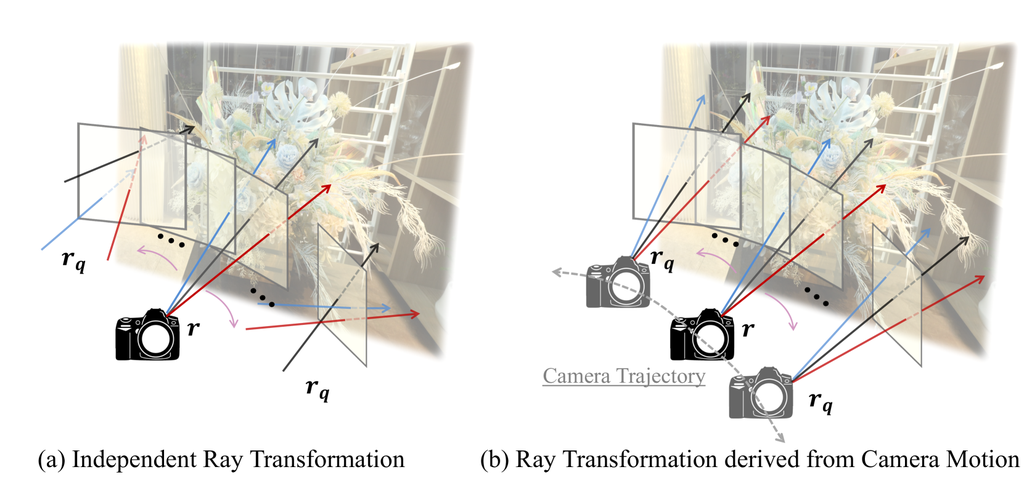
III-B Blur Kernels in Deblurred Neural Radiance Fields

The core difference of the blur kernels between the two papers is a consideration of 3D consistency across the entire pixels in each image as we describe in Figure 1. Deblur-NeRF [1] designs the blur kernel as a deformable sparse kernel (DSK), which consists of the $n$ number of transformations depending on embedded latent features from each view and location of image pixels. The transformation is formulated as the 3D vector of ray origin and 2D vector of pixel coordinate, which is initialized within $N\times N$ window on the image plane as

$${(\mathrm{\Delta }{\text{v}}_o,\mathrm{\Delta }{\text{v}}_T,m)}_q=G_{\mathrm{\Phi }}(\chi ,{\text{l}}_s),whereq\in \{1,\mathrm{\dots },n\}.$$ (9)

For $G_{\mathrm{\Phi }}$, MLP with parameter $\mathrm{\Phi }$, inputs are $\chi$ and ${\text{l}}_s$, which are latent embedded pixel coordinates and scene information, respectively. Here, $\chi$ is defined as randomly initialized canonical coordinates within a specific small range and $s$ indicates the specific scene. The 3D vector $\mathrm{\Delta }{\text{v}}_{\text{o}}$ and $\mathrm{\Delta }{\text{v}}_T$ transform given ray $\text{r}=\text{o}+t\text{d}$ to generate transformed rays imitating blurring process as Eq.10.

$${\text{r}}_q=(\text{o}+\mathrm{\Delta }{\text{v}}_{\text{o};q})+t{\text{d}}_q,$$ (10)

where ${\text{d}}_q$ is transformed ray direction by applying $\mathrm{\Delta }{\text{v}}_{T;q}$ to pixel coordinates to move the endpoint of the ray. Then blurred color $\widehat{B}$ of the target pixel is composited by weighted summation of each rendered color ${\widehat{C}}_q$ and $m_q$ as Eq.7.

However, DP-NeRF [2] argues that the pixel-wise independent optimization of the blur kernel in [1] incurs inconsistency in 3D geometry and appearance. They utilize the physical intuition of actual blurred image acquisition in the camera process as an additional prior for the DeRF, to impose the constraints for constructing radiance fields while preserving 3D consistency. To directly model the actual camera motion as a 3D rigid transformation, they introduce scene-wise $SE(3)$ fields inspired by [29], [49] and Rodrigues’ formula [50]. Scene-wise rigid transformation of the camera is formulated by estimated screw axis $S_s\in {ℝ}^6$ through MLPs depending on only scene information as Eq.11.

$$(S_{s;q},m_s)={(r_s,v_s,m_s)}_q=T_{\mathrm{\Psi }}({\text{l}}_s),whereq\in \{1,\mathrm{\dots },n\},$$ (11)

where $T_{\mathrm{\Psi }}$ and ${\text{l}}_s$ denote MLP with parameter $\mathrm{\Psi }$ and latent embedded scene information, respectively. The predicted $r_q$ and $v_q$ of $S_q$ are converted to rotation matrix $e^{r_q}$ and translation matrix ${\text{p}}_q$ by formulas of [50] and [49], respectively. Note that, we abbreviate specific scene indicator $s$ for clarity. Hence, transformed rays are formulated as the rigid transformation of the rays as Eq.12.

$${\text{r}}_q=e^{S_q}\text{r}=e^{r_q}\text{r}+{\text{p}}_q.$$ (12)

The blurred color $\widehat{B}$ of the target pixel is also composited by weighted summation of each rendered color ${\widehat{C}}_q$ and $m_q$ as same as Eq.7. In addition to modeling the blurring process with rigid blur kernel (RBK), [2] proposes an adaptive weight proposal network (AWP) based on the internal correlation between transformed rays and motion axis to predict the adaptive composition weights ${\tilde{m}}_q$ for each pixel, which complements the effect on the blur derived from the depth difference.

In this paper, we present a novel approach that includes geometric constraints and a perceptual prior through extensive experiments based on these two types of blur kernels from Ddeblur-NeRF [1] and DP-NeRF [2], which can be regarded as flexible and rigid kernels, respectively. The conducted experiments demonstrate the effectiveness of Sparse-DeRF on both kernels. Furthermore, the results also reveal a trade-off for the flexibility of the kernels, depending on the specific properties inherent in the diverse scenes.

IV Sparse-DeRF

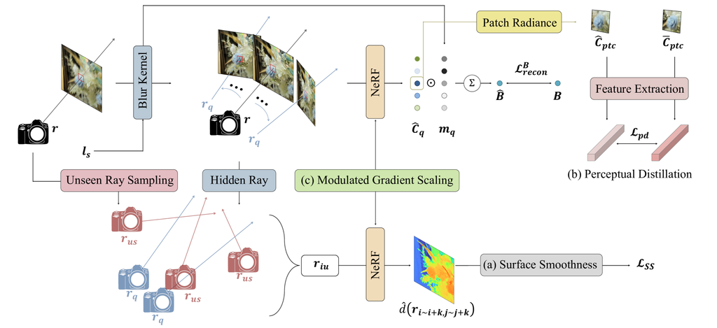
We find that it is not effective to construct the radiance fields based on naive NeRF, Deblur-NeRF [1], or DP-NeRF [2] from sparse view setting as we present in Section V-E. Although the DeRF usually recovers the high-frequency detail better than the naive NeRF in given views, it has become more fragmented in novel view synthesis, generating inaccurate scene geometry due to the complex joint optimization. The geometric error is represented as mapped RGB textures resembling painted walls in near or far depth and elongated density artifacts, which reveal challenges associated with accurate depth value prediction. However, existing representative regularization for the NeRF from sparse view [6] can not regularize complex joint optimization of the DeRF. We present experimental results in Section V-F1, which shows the difficulty of the previous regularization technique on the DeRF from sparse view. Hence, here we describe our method for regularizing optimization of the DeRF from sparse view to alleviate spatial ambiguity, which consists of two geometric constraints and a perceptual prior. Figure 2 illustrates the overall architecture of the Sparse-DeRF in detail, where (a),(b), and (c) of the Figure 2 indicate each main component of the Sparse-DeRF, respectively. Geometric constraints consist of surface smoothness (SS) and modulated gradient scaling (MGS) as we describe in Section IV-A and Section IV-B. A perceptual prior consists of a perceptual distillation (PD) which is described in Section IV-C.

Figure 2: Overall architecture of the Sparse-DeRF. Each color of integrated ray ${\text{r}}_{io}$ describes where the rays come from. ${\widehat{d}}_{\mathrm{\Theta }}({\text{r}}_{i\sim i+k,j\sim j+k})$ indicates the rendered depth patch with $k\times k$ size. Note that, $k$ is set to $S_{ptc}$ as we described in the paper. The main component of the Sparse-DeRF consists of (a) surface smoothness (SS), (b) perceptual distillation (PD), and (c) modulated gradient scaling (MGS), which are indicated as gray, pink, and green colored components.

Figure 3: Simple illustration of unobserved rays in our method, which consists of unseen rays and hidden rays. Two types of rays are independently defined. Unseen rays remain unchanged during training, but hidden rays change during the training since it is derived from the learned blur kernel. Note that, hidden rays can be derived from both types of blur kernel we utilized.

IV-A Surface Smoothness on Integrated Unobserved Rays

Inspired by the statistical tendencies of real-world geometry, piece-wise smoothness is adopted as a depth smoothness regularization on small rendered patches in RegNeRF [6]. This regularization can also be interpreted as imposing surface smoothness constraint, which is applied to the rendered depth obtained from unseen rays that are defined as rays not observed in the training inputs. The unseen rays are generated from possible camera locations sampled within a limited sample space, constrained by target poses for rendering during test time. Similar to the method introduced in [6], we adopted an approach to alleviate spatial ambiguity by utilizing information from unobserved rays. However, we propose additionally leveraging new unobserved ray information that can only be derived from the blur kernel to stabilize the simultaneous optimization of blur kernel and radiance fields. Firstly, we utilize unseen rays as one of the integrated unobserved rays to ameliorate spatial ambiguity following the [6]. For known set of camera poses ${\{{\text{P}}_{target}^i\}}_i$, where ${\text{P}}_{target}^i=[{\text{R}}_{target}^i|{\text{t}}_{target}^i]\in SE(3)$, sampled camera pose $S_{\text{P}}$ for unseen rays is formulated from camera location $S_{\text{t}}$ and rotation $S_{\text{R}}$ in limited sample space as

(13)

where ${\text{t}}_{min}$, ${\text{t}}_{max}$, ${\overline{\text{p}}}_u$, and ${\overline{\text{p}}}_f$ indicate $min(\{{\text{t}}_{target}^i\})$, $max(\{{\text{t}}_{target}^i\})$, the normalized mean over the up axes of all target poses, and the mean focus point by solving a least squares problem, respectively. $\text{R}(\cdot ,\cdot ,\cdot )$ and $ϵ$ indicate camera rotation matrix to make the sampled camera roughly focus on a central point of a scene and a small jitter value added to the focus point, respectively. To the end, sampled camera poses $S_{\text{p}}$ is formulated as

$$S_{\text{P}}=\{[\text{R}|\text{t}]|\text{R}\sim S_{\text{R}}|\text{t},\text{t}\sim S_{\text{t}}\}.$$ (14)

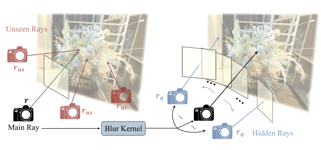
In addition to leveraging previously unseen rays, we employ hidden rays derived from the characteristics of the estimated blur kernel, harnessing supplementary information exclusively presented in blurry inputs. The blur kernel, denoted as $h$ in Eq. 6, generates the ray transformation to approximate the color composition process of the blur, regardless of the kernel types, as demonstrated in Deblur-NeRF [1] and DP-NeRF [2]. Motivated by the commonality in the color composition process across various blur kernels, the kernel-induced transformed rays ${\text{r}}_q$ are introduced as additional unobserved rays, which are referred to as hidden rays, to enforce depth smoothness constraint. As the hidden rays ${\text{r}}_q$ are not directly presented in the training data for the DeRF system, they serve as supplementary out-of-distribution data for imposing depth smoothness, similar to the aforementioned unseen rays. In addition, the incorporation of depth smoothness on hidden rays effectively addresses geometric inconsistency across the 3D space of blurry images within the specified training view. This capability stems from the broader coverage of the estimated hidden rays, facilitated by the implicit inclusion of camera motion information in blurry images. Therefore, our integrated unobserved rays for depth smoothness are defined as an integrated set of unseen rays and hidden rays as

$${\text{r}}_{iu}=\{{\text{r}}_q,{\text{r}}_{us}\},where{\text{r}}_q\sim h(\text{r}),{\text{r}}_{us}\sim S_{\text{p}},$$ (15)

where $r_{iu}$ and $r_{us}$ denote integrated unobserved rays and unseen rays, respectively. For more intuitive understanding, the ${\text{r}}_q$ and ${\text{r}}_{us}$ are illustrated in Figure 3.

For applying depth smoothness constraint on $r_{iu}$, the expected depth of $r_{iu}$ is computed following Eq.16 as same as previous NeRF works.

$$\widehat{d}={\int }_{t_n}^{t_f}T(t)\sigma (\text{r}(t))t𝑑t.$$ (16)

Then the depth smoothness loss is reformulated by adding color-dependent weighted depth smoothness from [6] as

${ℒ}_{ss}\{{\text{r}}_{iu}\}$ $={\displaystyle \sum _{\text{r}\in {\text{r}}_{iu}}}{\displaystyle \sum _{i,j=1}^{S_{ptc}-1}}[\mathrm{\Delta }{\widehat{d}}_x({\text{r}}_{i,j})+\mathrm{\Delta }{\widehat{d}}_y({\text{r}}_{i,j})],$ (17)

where $\mathrm{\Delta }{\widehat{d}}_x({\text{r}}_{i,j})$ and $\mathrm{\Delta }{\widehat{d}}_y({\text{r}}_{i,j})$ indicates horizontal and vertial weighted depth difference as Eq.18, respectively.

(18)

where ${\omega }_{i+k,j+1}=exp\left(-{\left(\widehat{C}({\text{r}}_{i,j})-\widehat{C}({\text{r}}_{i+k,j+l})\right)}^2\right)$ indicates pixel-wise color difference weight.

Figure 4: The comparison between ours modulated gradient scaling function with $\widehat{J}({\delta }_{{\text{s}}_i})$ and the previous function $J({\delta }_{{\text{s}}_i})$ proposed by [51], with respect to the ray distance ${\delta }_{{\text{s}}_i}$. In the table, the values of ${\delta }_{{\text{s}}_i}$ and $min(1,J({\delta }_{{\text{s}}_i}))$ on the x-axis and y-axis represent the ray distance from the camera origin and gradient scaling value, respectively. The $J({\delta }_{{\text{s}}_i})$ of [51] is represented as $x^2$ with the black colored line for clarity. The graphs illustrate that our modulated function $\widehat{J}({\delta }_{{\text{s}}_i})$ can cover the diversity in the arrangement of scene components, exhibiting various shapes of the function depending on magnitude $\rho$ and period $\eta$.

IV-B Modulated Gradient Scaling

Although previous surface smoothness alleviates the spatial ambiguity in the 3D scene, it is still hard to grasp accurate geometry due to the inherent drawback of the NeRF sampling strategy and casted volume occupancy as [51] argued. Following [51], the optimization of the NeRF often fails, generating the density artifact in the near-depth region due to the disproportionate gradient backpropagation induced from the imbalanced volumetric occupancy of the samples on the ray. [51] alleviates the limitation introducing gradient scaling that reduces the propagated gradient $\nabla {\text{s}}_i$ of each $i$-th sample ${\text{s}}_i=(s_x,s_y,s_z)$ on ray r according to the distance ${\delta }_{{\text{s}}_i}$ from ray origin o as

$$\nabla {\widehat{\text{s}}}_i=\nabla {\text{s}}_i\times min(1,J({\delta }_{{\text{s}}_i})),where{\delta }_{{\text{s}}_i}=|{\text{s}}_i-\text{o}|,$$ (19)

where $\nabla \widehat{{\text{s}}_i}$ and $J$ indicate scaled gradient value for sample $s_i$ and scaling function. The scaling function $J$ is strictly formulated as a squared function as

$$J({\delta }_{{\text{s}}_i})={({\delta }_{{\text{s}}_i})}^2.$$ (20)

Note that, $\nabla {\text{s}}_i$ indicates the gradients of per-point characteristics such as RGB color c and density $\sigma$.

However, we experimentally found that the limitation is more prominent in sparse view settings since there is less available diversity of viewing direction, which means the projective geometry and epipolar geometry do not properly work for NeRF optimization. Therefore, the gradient scaling seems to be more necessary to the radiance fields from the sparse view setting. Although we tried to apply the technique to the Sparse-DeRF, it does not properly works as demonstrated in the appendix. The reason is that the fixed square function of $J$, which is lower bounded as $1$, does not cover the non-linear parametrized space such as normalized device coordinates (NDC), which is commonly used as well as our work. Another reason is that a strictly fixed shape of the function cannot cover the arrangements of the scene components, which are usually different across the scene even in the same dataset. [51] briefly mentioned the determinant of the jacobian as an additional scaling factor for the value of $J$, but they did not experiment on it. Moreover, even if the additional scaling factor were applied, the shape of the scaling function would remain unchanged and simply in the form of the square function, which does not allow for flexible adaptation to the arrangement of scene components. Therefore, we modulate the shape of the scaling function $J$ to adaptively reflect the scene arrangements and be suitable for NDC.

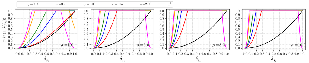
Our novel gradient scaling function $\widehat{J}$ is designed based on three conditions. First, the function should increase from zero at the camera origin, which is a critical condition to avoid the local minima in the initial training phase we mentioned before. Second, the function should be not zero in the far distance, which is set to $1$ in our NDC environment, to ensure the NeRF training. Finally, the function is designed to increase and decrease only once within a given depth range, which makes the function not fluctuate, since it is an intuitively reasonable scenario considering the goal of MGS that alleviates incorrect density mapping in near distance. In addition to the above conditions for proper shape of the scaling function, we further consider designing the function shape when the location of the main objects is focused on the center of the scene and density mapping error that is represented as a painted wall of near or far depth. Following the conditions, the proposed modulated gradient scaling (MGS) function $\widehat{J}$ is formulated as

$$\widehat{J}({\delta }_{{\text{s}}_i})=\rho \left(\sin \left(\eta \pi ({\delta }_{{\text{s}}_i}+\frac{3}{2\eta })\right)+1\right),$$ (21)

where $(1\le \rho \le 10)$ and denote magnitude and period of sinusoidal function, respectively. However, in contrast to [51], the distance range of ${\delta }_{{\text{s}}_i}$ is restricted to ${\delta }_{{\text{s}}_i}\in [0,1]$ since we use NDC for our dataset.

To apply gradient scaling both in the near and far regions while minimizing the scaling effect in the center of the scene, we adopt the sinusoidal function shape as the foundation for our MGS. Furthermore, the second condition determines the maximum value of $\eta$ as 2 to ensure the scaling value of the proposed function in the far region does not fall to or below 0. The function shape in the left top image of Figure 4 shows the characteristics of the proposed scaling function that we described above. We shows the difference between the scaling value from $min(1,J({\delta }_{{\text{s}}_i}))$ and $min(1,\widehat{J}({\delta }_{{\text{s}}_i}))$, according to the various $\rho$ and $\eta$ values in Figure 4.

Figure 5: Illustration of our perceptual distillation. Perceptual distillation transfers the information of pre-deblurred texture by applying the perceptual loss to the pre-deblurred color patch ${\overline{C}}_{ptc}$ and rendered color patch ${\widehat{C}}_{ptc}$, which is rendered from patch-wise sampled rays ${\text{r}}_{ptc}^{pd}$ in same pixel location. Note that ${\mathrm{\Theta }}_D$ and $ℰ$ are pre-trained image deblurring network and a shared pre-trained image feature extractor, respectively.

IV-C Perceptual Distillation

In contrast to the previous NeRF-related works in sparse view settings, the Sparse-DeRF environments enable to use the off-the-shelf image processing algorithms, such as deep learning-based image deblurring networks, due to the degradation of the given images. In addition to improvements from a geometric perspective, we aim to enhance the detailed textures of DeRF utilizing the advantages of existing image processing modules, thereby achieving high fidelity.

However, it is not possible to directly utilize the pre-deblurred images as additional pixel-wise color supervision, due to the lack of 3D consistency. This inconsistency occurs due to the ill-posed property of image deblurring and independent deblurring processing across multi-view images, which generates incoherent deblurred results. In the appendix, we additionally address this issue and present the qualitative comparison of pre-deblurred images and reference images, which are estimated from the DP-NeRF [2] trained with the full view, to reveal the geometric inconsistency issue.

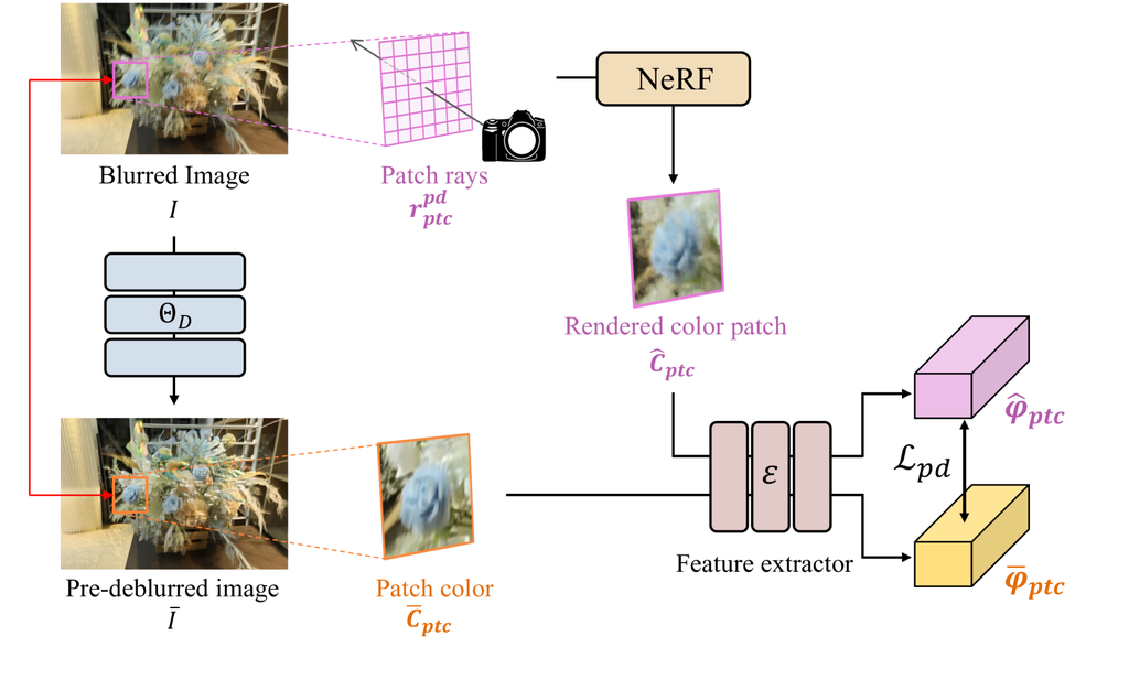
To overcome the intrinsic inconsistency of pre-deblurred images, we address the pre-filtered images as a perceptual prior, which transfers the deblurred texture information by extracting features from rendered patches and deblurred images with a pre-trained feature extractor. Figure 5 simply illustrates the pipeline of our perceptual distillation module.

Specifically, we first generate deblurred images $\overline{I}$ for blurry training images $I$ by exploiting a pre-trained image deblurring network ${\mathrm{\Theta }}_D$ to prepare the feature extraction as

$$\overline{I}={\mathrm{\Theta }}_D(I)$$ (22)

Next, we additionally sample the $S_{ptc}^{pd}\times S_{ptc}^{pd}$ size of patch rays ${\text{r}}_{ptc}^{pd}$ and corresponding deblurred image patch ${\overline{C}}_{ptc}$ from $\overline{I}$ on training views. Then we extract the abundant deblurred features from the rendered color patch ${\widehat{C}}_{ptc}$, which is rendered from ${\text{r}}_{ptc}^{pd}$, and pre-deblurred images $\overline{I}$ using a shared pre-trained image feature extractor $ℰ$ as

$${\widehat{\phi }}_{ptc}=ℰ({\widehat{C}}_{ptc}),{\overline{\phi }}_{ptc}=ℰ({\overline{C}}_{ptc}),$$ (23)

where ${\widehat{\phi }}_{ptc}$ and ${\overline{\phi }}_{ptc}$ indicate extracted features from each color patches, respectively. Note that, the color patch ${\widehat{C}}_{ptc}$ is rendered by forwarding the NeRF MLPs without blur kernel to perceptually transfer the pre-filtered texture information to the implicit clean radiance fields, which is indicated as patch radiance in Figure 2. Then we apply the perceptual loss ${ℒ}_{pd}$ [52] to distill the feature information as

$${ℒ}_{pd}={\Vert {\widehat{\phi }}_{ptc}-{\overline{\phi }}_{ptc}\Vert }_2^2.$$ (24)

Our final loss function is a weighted composition of the proposed losses as

$${ℒ}_{final}={ℒ}_{recon}^B+{\lambda }_{ss}{ℒ}_{ss}+{\lambda }_{pd}{ℒ}_{pd},$$ (25)

where ${\lambda }_{ss}$ and ${\lambda }_{pd}$ denote weights for each loss, which are equally set to $0.01$ in our experiments.

V Experiments

V-A Dataset

Sparse-DeRF has experimented with a forward-facing scene dataset proposed by Deblur-NeRF [1], which includes 5 synthetic and 10 real scenes. In particular, we use only the camera motion blur dataset since our goal is to alleviate the blur from camera motion in the DeRF from sparse view settings. The dataset consists of multiple view images and paired camera poses calibrated by using COLMAP [53, 54]. For the sparse view setting, we manually select the 2, 4, and 6 images as training datasets for all scenes, so that the entire space covered by each view is as wide as possible. In addition, to ensure reasonable learning of radiance fields, we select views with visible spaces that overlap as little as possible, while avoiding excessively extreme blur magnitudes. Note that, it is an inherent property of the dataset that blur magnitudes of selected views can be different according to each scene, which means that each scene has a different level of learning difficulty. We attach the selected image indices of all scenes used in our experiments in the appendix for fair comparison in future research.

V-B Experimental Sparse View Setting

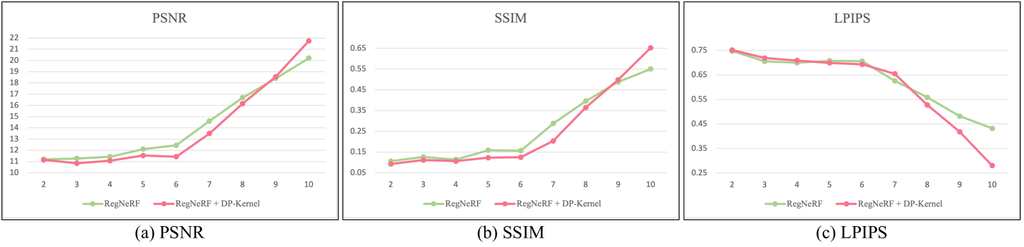
Scenarios for the Sparse-DeRF are assumed to be three kinds of settings, which are the DeRF from 2-view, 4-view, and 6-view settings unlike existing common sparse-view NeRFs, which usually use 3-view, 6-view, and 9-view settings. The reason is that when using more than 8 images, the joint optimization problem occurs more frequently under 9-view settings as shown in Figure 6. The figure presents the graph of experiments in the Decoration scene where we varied the number of input sparse views from 2-view to 10-view. We also attach the quantitative results in the appendix due to the page limitation. Experimental results reveal that our sparse-view experimental settings are valid since the RegNeRF [6] with DP-kernel shows poor performances under the 9 views.

V-C Implementation Details

Spare-DeRF is implemented and modified based on the published official code of DP-NeRF [2] using the two types of blur kernels of DP-NeRF [2] and Deblur-NeRF [1]. For a fair comparison, the number of blurring rays is set to $5$ for the default setting as same as previous works [1, 2]. We set the other settings for the blur kernels following the default parameters of each work. For the NeRF optimization, we use $64$ coarse and $64$ fine samples per ray with a batch size of 1024 rays, exploiting Adam [55] optimizer with default parameters. In addition, exponential weight decay is applied from $5\times {10}^{-4}$ to $8\times {10}^{-5}$ for learning rate scheduling. We train the DeRF for $20k$, $40k$, and $60k$ iterations in 2-view, 4-view, and 6-view settings, respectively. For patch-wise sampling, we set the size of the patch $S_{ptc}$ and $S_{ptc}^{pd}$ as $8$ and $64$, respectively. However, the generating method of unseen rays in surface smoothness constraint is especially considered for fair comparison across the extensive experiments. In particular, we generate the unseen rays from fixed views, which are evenly selected from the rest of the training rays, to remove the randomness of the unseen ray generation for experimental analysis and fair comparison. Note that, the rest of the training rays are not included in the training or test view. We demonstrate that it is a reasonable choice since the selected views are still in the sample space we defined in Section IV-A. In addition, we attach the visualization of this issue in the appendix to show the rationality. The hyper-parameters of the modulated gradient scaling function for each scene, magnitude $\rho$ and period $\eta$, are attached in the appendix in detail. For perceptual distillation, MPRNet [56] is utilized as a pre-trained image deblurring network. We select the VGG19 [57] as a pre-trained image feature extractor $ℰ$ since it is widely exploited as an image feature extractor in image-based computer vision.

V-D Evaluation Metrics

Our experimental results for the synthetic and real datasets are evaluated in three quantitative metrics and qualitative comparisons between rendered images through a novel view synthesis task. Consistent with prior research, we employ widely utilized evaluation metrics to compare the synthesized images with corresponding ground truth images: the peak signal-to-noise ratio (PSNR), the structural similarity index measure (SSIM), and learned perceptual image patch similarity (LPIPS) [58]. These metrics assess the relative sharpness, structural similarity, and perceptual quality of the generated images, respectively. In addition, we encourage readers to refer to the supplementary video for a more comprehensive and detailed presentation of the results.

Figure 6: Graph of the experimental results of Decoration scene from 2-view to 10-view settings. Figure (a), (b), and (c) indicate PSNR, SSIM, and LPIPS, respectively. The graph reveals that the network suffers joint optimization problems under the 9-view setting, which makes our experimental setting plausible.

V-E Evaluation

TABLE I: Average results of novel view synthesis for both synthetic and real scenes obtained from 2-view, 4-view, and 6-view settings. Each color shading represents the best, second best, and third best result for each experimental setting, respectively.

	[ 2-view ]						[ 4-view ]						[ 6-view ]
	[ Synthetic Scene ]			[ Real Scene ]			[ Synthetic Scene ]			[ Real Scene ]			[ Synthetic Scene ]			[ Real Scene ]
	PSNR($\uparrow$)	SSIM($\uparrow$)	LPIPS($\downarrow$)	PSNR($\uparrow$)	SSIM($\uparrow$)	LPIPS($\downarrow$)	PSNR($\uparrow$)	SSIM($\uparrow$)	LPIPS($\downarrow$)	PSNR($\uparrow$)	SSIM($\uparrow$)	LPIPS($\downarrow$)	PSNR($\uparrow$)	SSIM($\uparrow$)	LPIPS($\downarrow$)	PSNR($\uparrow$)	SSIM($\uparrow$)	LPIPS($\downarrow$)
Naive NeRF [19]	15.11	.2999	.5578	14.38	.2635	.6004	20.02	.5327	.4000	18.98	.4860	.4481	21.65	.5985	.3638	20.63	.5513	.4014
MPR [56] + NeRF	15.16	.3006	.5595	14.38	.2594	.6019	20.00	.5381	.3956	18.89	.4829	.4484	21.72	.5999	.3629	20.60	.5513	.4010
Deblur-NeRF [1]	15.14	.2884	.5330	14.41	.2506	.5921	19.99	.5199	.3499	18.89	.4761	.4151	23.12	.6798	.2386	21.36	.6003	.3163
DP-NeRF [2]	15.06	.2827	.5389	14.36	.2506	.5904	19.84	.5336	.3075	18.77	.4582	.4175	23.68	.7036	.1998	21.68	.6137	.2992
RegNeRF [6] (No kernel)	14.60	.2849	.5869	15.49	.2997	.5888	18.39	.4600	.4704	18.44	.4326	.4852	19.69	.5249	.4165	19.65	.4790	.4583
RegNeRF [6] (w/DP-kernel)	13.24	.2162	.6062	12.76	.1836	.6447	16.44	.3657	.4826	13.59	.2221	.5887	21.60	.6162	.3046	18.25	.4439	.4326
Sparse-DeRF (w/DN-kernel) - Ours	15.52	.2966	.5291	15.53	.3112	.5515	20.57	.5565	.3354	19.98	.5231	.3871	23.32	.6903	.2379	22.15	.6248	.3030
Sparse-DeRF(w/DP-kernel) - Ours	15.35	.2904	.5242	15.57	.3114	.5467	21.05	.5776	.2975	20.05	.5178	.3736	24.27	.7255	.2044	22.32	.6283	.2907

Figure 7: Qualitative results on Parterre, Coffee, and Decoration scene from (a) 2-view, (b) 4-view, and (3) 6-view respectively. (i), (ii), and (iii) denote rendered color and depth images from DP-NeRF [2], RegNeRF [6] with DP-kernel, and Ours(Sparse-DeRF) with DP-kernel.

V-E1 Quantitative Evaluation

We present the quantitative results of Sparse-DeRF for two different types of blur kernels from Deblur-NeRF [1] and DP-NeRF [2], comparing these results with established baseline methods. The effectiveness of our approach is demonstrated in TABLE I, achieving outstanding performance across entire sparse view settings, regardless of the blur kernel employed. In the Sparse-DeRF results, DN-kernel and DP-kernel denote the blur kernels proposed by the Deblur-NeRF [1] and DP-NeRF [2], respectively. MPR$+$NeRF denotes the naive NeRF model trained solely on color supervision from deblurred images by MPRNet [56], utilizing the reconstruction loss ${ℒ}_{recon}$ of Eq.5. The results of MPR$+$NeRF reveal interesting observations and marginal improvements in radiance fields when only employing pre-deblurred images as direct color supervision for training. This tendency emphasizes the 3D inconsistency across the pre-deblurred images, as discussed in Section IV-C. In addition, the poor results of the RegNeRF [6] with and without a blur kernel demonstrate that existing regularization faces difficulty in alleviating the complex joint optimization involving both the blur kernel and radiance fields. We further present an analysis of this optimization issue in Section V-F1 with detailed experimental results. In contrast, Sparse-DeRF demonstrates significant enhancements across all evaluation metrics for both types of blur kernels, indicating its superior ability to represent the DeRF with improved visual quality. In particular, our results exhibit more prominent improvements in real-scene scenarios, although there is non-ideal blur degradation, which occurs due to various real environmental factors. For a comprehensive understanding, we provide an extensive ablation study in Section V-F, incorporating results with both types of blur kernels. Additionally, detailed results for all scenes are appended in the appendix, including synthetic and real scenes.

V-E2 Qualitative Evaluation

In Figure 7, we present representative qualitative results on three scenes (Parterre, Coffee, and Decoration) from 2-view, 4-view, and 6-view settings, respectively. The figure depicts the results of novel view synthesis, presenting rendered color and depth images. The figures demonstrate that our model significantly enhances the visual quality of radiance fields in terms of geometric and perceptual fidelity. In addition to the above quantitative results, qualitative results also demonstrate the inconsistency issue of pre-deblurred images and complex joint optimization of the DeRF from sparse view. All the results (ii) of Figure 7 demonstrate that existing representative regularization technique, RegNeRF [6], can not effectively alleviate the optimization issue of the DeRF from sparse view. Furthermore, we encourage readers to view the supplementary videos that emphasize 3D consistency through rendered videos from a spiral camera path.

V-F Ablations

V-F1 Problem Analysis and Motivation

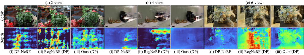
we present the experimental results to describe that it is difficult to jointly optimize the DeRF and naively apply the previous regularization technique of the NeRF to the DeRF from sparse view setting, utilizing the representative existing regularization method, RegNeRF [6]. We attach the experimental results of the RegNeRF [6] from 2-view, 4-view, and 6-view settings with and without the blur kernel to demonstrate the difficulty of the complex joint optimization problem as we mentioned. TABLE II and Figure 8 present quantitative and qualitative results from 2-view, 4-view, and 6-view, respectively. The blur kernel employed is the rigid blur kernel of DP-NeRF [2], which is described as DP-kernel in the table and figures. To help the reader compare the plausible appearance and dense geometry with the proposed Sparse-DeRF, we attach the rendered color and depth images of our model. The results of the figures demonstrate that the integration of the blur kernel involves a straightforward difficulty in optimizing the high-frequency details and the overall scene geometry simultaneously, as indicated by the visual quality of the rendered color and depth images. Although the presence of a blur kernel enables radiance fields to capture high-frequency details, it causes a geometric distortion with the overall wrong density mapping that resembles the fragmented structure of objects or appearance like the painted wall of near- or far-depth regions. These results and analysis demonstrate that naively applying the regularization of the NeRF from sparse view to the DeRF is not effective. In addition, the images (i) and (ii) in Figure 8 demonstrate that although the overall performance is better without the blur kernels, the model still faces difficulty in modeling high-frequency details. This difficulty makes the necessity of the blur kernel optimization still important, leading to a blurry visual quality across the entire scene. Therefore, motivated by the experimental analysis, we propose Sparse-DeRF, the novel regularization method for optimization of the blur kernel and radiance fields simultaneously. The proposed Sparse-DeRF presents high-quality rendered images with dense geometry and detailed high-frequency texture as shown in Figure 8.

TABLE II: Average results for the complex optimization issue in both synthetic and real scenes from 2-view, 4-view, and 6-view settings. Each color shading represents the best and second results for each experimental setting, respectively.

		[ 2-view ]						[ 4-view ]						[ 6-view ]
		[ Synthetic Scene ]			[ Real Scene ]			[ Synthetic Scene ]			[ Real Scene ]			[ Synthetic Scene ]			[ Real Scene ]
	Blur Kernel	PSNR($\uparrow$)	SSIM($\uparrow$)	LPIPS($\downarrow$)	PSNR($\uparrow$)	SSIM($\uparrow$)	LPIPS($\downarrow$)	PSNR($\uparrow$)	SSIM($\uparrow$)	LPIPS($\downarrow$)	PSNR($\uparrow$)	SSIM($\uparrow$)	LPIPS($\downarrow$)	PSNR($\uparrow$)	SSIM($\uparrow$)	LPIPS($\downarrow$)	PSNR($\uparrow$)	SSIM($\uparrow$)	LPIPS($\downarrow$)
RegNeRF [6]	$\times$	14.60	.2849	.5869	15.49	.2997	.5888	18.39	.4600	.4704	18.44	.4326	.4852	19.69	.5249	.4165	19.65	.4790	.4583
RegNeRF [6]	DP-kernel	13.24	.2162	.6062	12.76	.1836	.6447	16.44	.3657	.4826	13.59	.2221	.5887	21.60	.6162	.3046	18.25	.4439	.4326
Sparse-DeRF (Ours)	DP-kernel	15.35	.2904	.5242	15.57	.3114	.5467	21.05	.5776	.2975	20.05	.5178	.3736	24.27	.7255	.2044	22.32	.6283	.2907

Figure 8: Qualitative results on Pool, Tanabata, and Heron scene for complex optimization issue from 2-view, 4-view, and 6-view settings. (i), (ii), and (ii) denote the rendered images from the RegNeRF [6] with no blur kernel, RegNeRF with DP-kernel, and Sparse-DeRF(Ours) with DP-kernel, respectively.

TABLE III: Ablation experimental results from 2-view, 4-view, and 6-view according to the proposed geometric constraints and perceptual prior, denoted in the table as surface smoothness (SS), modulated gradient scaling (MGS), and perceptual distillation (PD), respectively. We present separate results for our model with both types of kernels, DP-kernel [2] and DN-kernel [1]. Each color shading represents the best, second best, and third best result for each experimental setting, respectively.

				[ 2-view ]						[ 4-view ]						[ 6-view ]
	SS	MGS	PD	DP-kernel			DN-kernel			DP-kernel			DN-kernel			DP-kernel			DN-kernel
				PSNR($\uparrow$)	SSIM($\uparrow$)	LPIPS($\downarrow$)	PSNR($\uparrow$)	SSIM($\uparrow$)	LPIPS($\downarrow$)	PSNR($\uparrow$)	SSIM($\uparrow$)	LPIPS($\downarrow$)	PSNR($\uparrow$)	SSIM($\uparrow$)	LPIPS($\downarrow$)	PSNR($\uparrow$)	SSIM($\uparrow$)	LPIPS($\downarrow$)	PSNR($\uparrow$)	SSIM($\uparrow$)	LPIPS($\downarrow$)
Synthetic Scene				15.06	.2827	.5389	15.14	.2884	.5330	19.84	.5336	.3075	19.99	.5199	.3499	23.68	.7036	.1998	23.12	.6798	.2386
	✓			14.88	.2772	.5388	15.25	.2828	.5418	19.93	.5411	.3107	19.89	.5201	.3558	24.15	.7263	.1974	23.59	.6795	.2429
		✓		15.40	.2857	.5289	15.12	.3025	.5243	20.16	.5425	.3024	19.44	.5295	.3562	23.83	.7147	.2072	24.33	.6832	.2406
			✓	15.03	.2796	.5391	14.84	.2702	.5454	19.65	.5237	.3311	19.72	.5104	.3630	23.89	.7150	.2052	23.35	.6941	.2341
	✓		✓	14.52	.2647	.5481	15.11	.2889	.5389	20.91	.5812	.2948	20.03	.5294	.3450	24.28	.7279	.2021	23.41	.6941	.2324
	✓	✓		15.50	.2954	.5215	15.57	.2979	.5319	19.65	.5164	.3334	19.96	.5222	.3547	23.53	.7088	.2153	22.91	.6654	.2560
	✓	✓	✓	15.35	.2904	.5242	15.52	.2966	.5291	21.05	.5776	.2975	20.57	.5565	.3354	24.27	.7255	.2044	23.32	.6903	.2379
Real Scene				14.36	.2506	.5904	14.41	.2506	.5921	18.77	.4582	.4175	18.89	.4761	.4151	21.68	.6137	.2992	21.36	.6003	.3163
	✓			14.26	.2414	.5933	14.33	.2495	.5937	19.04	.4760	.4008	18.96	.4839	.4125	22.10	.6214	.2951	21.53	.6044	.3178
		✓		15.46	.3035	.5465	15.44	.3037	.5558	19.75	.4980	.3737	19.06	.4907	.4105	22.07	.6212	.2889	21.76	.6101	.3097
			✓	14.28	.2490	.5896	14.47	.2549	.5939	19.00	.4724	.4080	19.84	.5118	.3937	21.73	.6082	.3082	21.69	.6087	.3142
	✓		✓	14.00	.2587	.5830	14.47	.2563	.5881	19.00	.4760	.4037	18.94	.4861	.4145	21.84	.6105	.3084	21.70	.6129	.3144
	✓	✓		15.40	.3009	.5527	15.46	.3073	.5519	19.74	.4986	.3774	19.93	.5188	.3873	22.22	.6257	.2868	21.88	.6154	.3112
	✓	✓	✓	15.57	.3114	.5467	15.53	.3112	.5515	20.05	.5178	.3736	19.98	.5231	.3871	22.32	.6283	.2907	22.15	.6248	.3030

Figure 9: Qualitative ablation results of each component on Girl, Stair, and Coffee scenes from 2-view, 4-view, and 6-view settings, respectively. We attach the rendered depth images of the DP-NeRF [2] trained from full view as reference depth images to help the reader compare the results.

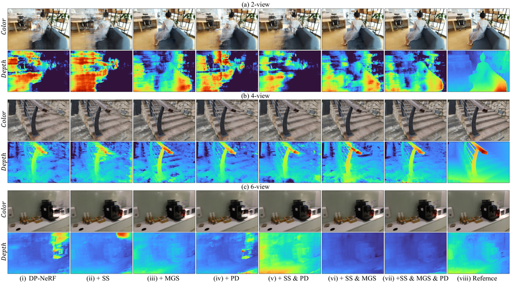
V-F2 Ablation of Each Component

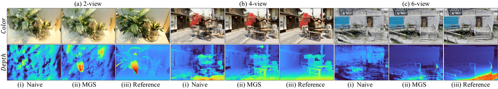
We demonstrate the effectiveness of the Sparse-DeRF’s each component through comprehensive ablation studies, presenting both quantitative and qualitative results. In TABLE III and Figure 9, we present independent quantitative and qualitative results from SS, MGS, and PD, where each component is individually applied to observe the influence of each method. The results include several combinations of the components to reveal the complement effect of each proposed method. The experiments are conducted for entire 2-view, 4-view, and 6-view settings, providing a different performance depending on two types of blur kernels, DN-kernel [1] and DP-kernel [2]. Our model shows superior results in predicting both 3D geometric and appearance details precisely, demonstrating the enhanced evaluation results.

V-F3 Ablation Analysis

Quantitative ablation results demonstrate that our model with full components shows the best results in the real-scene dataset. The results reveal that MGS plays an important role across the entire 2-view, 4-view, and 6-view settings among geometric constraints although each constraint enhances the geometric accuracy. In Figure 9, the importance of MGS is more clearly prominent with qualitative results as color and depth images. If MGS is not applied, we can see that the geometry of the scene is not accurately captured or there are many density artifacts. On the other hand, PD seems to be not effective without geometric constraints in 2-view and 4-view settings as we can figure out in TABLE III and Figure 9. The reason is that the NeRF has more difficulty in predicting the correct geometry with only pre-deblurred images due to the inherent 3D inconsistency, which makes perceptual prior not effective. These difficulties become more severe as the number of views decreases. We can demonstrate that a certain level of accurate geometry should be achieved before applying perceptual distillation.

TABLE IV: Average quantitative comparison results between naive gradient scaling of [51] and our MGS in both synthetic and real scenes from 2-view, 4-view, and 6-view settings. The two types of kernels we utilize in this paper are indicated as DP-kernel and DN-kernel, the kernels of DP-NeRF [2] and Deblur-NeRF [1], respectively. Color shading represents the better result.

		[ 2-view ]						[ 4-view ]						[ 6-view ]
		[ Synthetic Scene ]			[ Real Scene ]			[ Synthetic Scene ]			[ Real Scene ]			[ Synthetic Scene ]			[ Real Scene ]
Blur Kernel	Gradient Scaling	PSNR($\uparrow$)	SSIM($\uparrow$)	LPIPS($\downarrow$)	PSNR($\uparrow$)	SSIM($\uparrow$)	LPIPS($\downarrow$)	PSNR($\uparrow$)	SSIM($\uparrow$)	LPIPS($\downarrow$)	PSNR($\uparrow$)	SSIM($\uparrow$)	LPIPS($\downarrow$)	PSNR($\uparrow$)	SSIM($\uparrow$)	LPIPS($\downarrow$)	PSNR($\uparrow$)	SSIM($\uparrow$)	LPIPS($\downarrow$)
DN-kernel	+ Naive [51]	14.70	.2483	.5643	14.85	.2860	.5653	18.69	.4321	.4242	19.28	.4909	.4119	22.00	.6002	.3117	21.20	.5877	.3274
DN-kernel	+ MGS	15.12	.3025	.5243	15.44	.3037	.5558	19.44	.5295	.3562	19.84	.5118	.3937	22.40	.6832	.2406	21.76	.6101	.3097
DP-kernel	+ Naive [51]	14.01	.2377	.5743	14.95	.2871	.5591	17.25	.3933	.4221	18.85	.4670	.4014	21.55	.6097	.2838	21.49	.6010	.3111
DP-kernel	+ MGS	15.40	.2857	.5289	15.46	.3035	.5465	20.16	.5425	.3024	19.75	.5980	.3737	23.83	.7147	.2072	22.07	.6212	.2889

Figure 10: Qualitative results on Puppet, Trolley, and Factory scene for comparison between naive gradient scaling [51] and our proposed MGS from 2-view, 4-view, and 6-view settings. Note that we attach the rendered color and depth images from DP-NeRF [2] trained with full view as reference images.

V-F4 Comparison to Naive Gradient Scaling

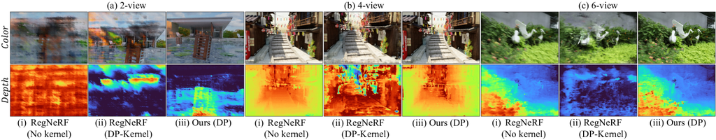
We present experimental results of quantitative and qualitative comparison between our proposed MGS and naive gradient scaling of [51] from 2-view, 4-view, and 6-view settings in TABLE IV and Figure 10. We compare the effectiveness of our MGS for two types of kernels we utilize in our paper, which are the kernels of Deblur-NeRF [1] and DP-NeRF [2]. The results describe our MGS outperforms the naive gradient scaling in terms of both quantitative and qualitative performance across the entire experimental setting. Specifically, depth images demonstrate that our MGS more effectively helps the model to predict the accurate geometry than naive gradient scaling. Quantitative results for the entire scene are attached in the appendix.

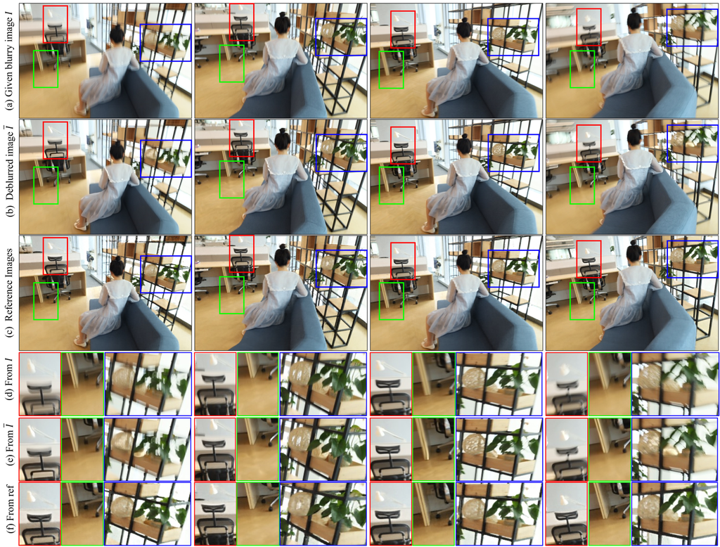
V-F5 Inconsistency of Pre-deblurred Images

As mentioned in Section I and IV-C, image deblurring is conducted independently for each image and presents inconsistent geometry in various regions due to its ill-posed property. In Figure 11, we present the qualitative comparison to reveal the inconsistency of pre-deblurred images across the multi-view training images. Pre-deblurred images are acquired by applying the MPRNet [56]. In addition, we attach the reference images, which are rendered from the DP-NeRF [2] trained with full view, to help readers better understand the inconsistency issue and compare the pre-deblurred geometry to approximated ground truth geometry. Comparing emphasized regions from each image, the pre-deblurred image shows relatively well-restored textures in each image, but the geometry is inconsistently restored and distorted across the multiple views. Such inconsistency adversely affects the learning of radiance fields since it is trained by pixel-wise color reconstruction loss. Furthermore, the performance of image deblurring varies even within a single image depending on the structural complexity of the local region, making it challenging to learn blur kernels. Due to these reasons, directly utilizing pre-filtered images for training radiance fields is difficult. Therefore, perceptual distillation is introduced to transfer only the perceptual texture of pre-deblurred images to the radiance fields.

Figure 11: Qualitative comparison on Girl scene that demonstrates the geometric inconsistency of pre-deblurred images. Figure (a)$\sim$(c) presents input blurry images $I$ for training, pre-deblurred images $\overline{I}$ by MPRNet [56], and rendered images from DP-NeRF [2] trained with full view, respectively. Figure (d)$\sim$(f) shows the emphasized regions of Figure (a)$\sim$(c), which demonstrates the inconsistency issue in detail.

VI Limitations and Discussions

Despite the remarkable enhancement in terms of 3D geometry and appearance, there are still several limitations. The first one is derived from the blur kernel itself, especially the relationship between the type of the blur kernel and the properties of each scene. For example, the performance is more improved with the rigid blur kernel of DP-NeRF [2] in some scenes, but in other scenes, the improvements are greater with the flexible blur kernel of Deblur-NeRF [1]. These kernel-dependent performances are different across the scenes. As we figure out, a flexible kernel leads to reduced space ambiguity but high scene distortion. In contrast, the rigid kernel leads to accurate geometry but suffers difficulty in optimizing the scene where the distances of the objects from the camera in the scene are diverse and some objects are located very close to the camera due to the inherent rigidity. We tried to take advantage of both kernels and design the hybrid kernel to maximize the effectiveness of the Sparse-DeRF, but it didn’t work as we imagined. Constructing the hybrid blur kernel that has rigid and flexible properties can be a promising future research direction regardless of sparse view setting in the deblurred neural radiance fields (DeRF). The second one is that we have to set the proper hyper-parameter for MGS to find the most effective function shape although MGS greatly improves the 3D geometry in the DeRF from sparse view. However, it is difficult to find an ideal function shape according to the arrangement of the object in the scene, especially as we mentioned above. We handle these cases by setting the magnitude $\rho$ as a high value to only ignore the gradient in a very near distance region, which is attached to the appendix as detailed hyper-parameters per each scene. In this sense, this manual setting of hyperparameters is regarded as one of our limitations. We believe the limitation can be alleviated in future research through various methods such as the introduction of learnable parameters for gradient scaling function. Finally, although sparse view setting of blurry inputs is an extremely practical scenario for blurry inputs, it is too hard to enhance the performance of the DeRF in the 2-view setting due to the lack of the scene information included in the input data. The innate challenge of the 2-view setting is that sparse overlapped 3D space usually leads to inaccurate geometry, which is more likely to be mapped to be painted texture on the wall at the near or far depth regions. There is still room to improve the visual quality of the Sparse-DeRF and solve these problems through state-of-the-art generative methods such as diffusion models, which can be a great future direction for constructing the DeRF from sparse view.

VII Conclusion

In this work, we propose the Sparse-DeRF, a novel regularization method for high-quality deblurred neural radiance fields from sparse view settings, which considers more practical real-world scenarios for radiance fields from only blurry images. We propose two geometric constraints that consist of surface smoothness and modulated gradient scaling, which reflect the real-world statistical geometry and alleviate elongated density artifacts in deblurred neural radiance fields system from sparse view. In addition, we propose a perceptual distillation to utilize the pre-deblurred images as a perceptual prior, which enhances the sharp texture on deblurred neural radiance fields. We demonstrate the effectiveness of the Sparse-DeRF that ameliorates the spatial ambiguity and structural distortion of deblurred neural radiance fields by presenting extensive experimental results in 2-view, 4-view, and 6-view settings. As deblurred neural radiance fields have attracted attention across the research fields related to neural rendering, we believe our work presents a way for future research directions since we address the more practical scenarios for deblurred neural radiance fields from blurry images.

Dogyoon Lee is a Ph.D candidate at the School of Electrical and Electronic Engineering, Yonsei University. He received his B.S. degree in Electrical and Electronic Engineering from Yonsei University, Seoul, South Korea, in 2019. His current research interests focus on 3D computer vision including Neural rendering and its applications in real-world scenarios, 3D from Images, 3D generative models, 3D reconstruction, and Image processing.

Donghyeong Kim is a Ph.D candidate at the School of Electrical and Electronic Engineering, Yonsei University. He received his B.S. degree in Electrical and Electronic Engineering from Yonsei University, Seoul, South Korea, in 2021. degree. His current research interests include anomaly detection, 3D computer vision, generative models, 3D reconstruction, and Image processing.

Jungho Lee is a Ph.D candidate at the School of Electrical and Electronic Engineering, Yonsei University. He received his B.S. degree in Electrical and Electronic Engineering from Yonsei University, Seoul, Korea, in 2021. His current research interests focus on neural rendering and human motion analysis in real-world conditions, with various mathematical machine learning tools such as neural ordinary differential equations.

Minhyeok Lee is a dedicated Computer Vision and ML/DL Researcher with a focus on segmentation, autonomous driving, detection & recognition, and novel view synthesis. Currently pursuing an Integrated M.S./Ph.D. in Electrical and Electronic Engineering at Yonsei University. His research spans various areas such as salient object detection, video object segmentation, camouflaged object detection, lane detection, and monocular depth estimation.

Seunghoon Lee received the B.S degree in Electronic Engineering of Inha University, Incheon, Korea in 2020. He is currently an integrated MS/Ph.D degree student in Electrical and Electronic Engineering, at Yonsei University. His research interests are video object segmentation, salient object detection, and super-resolution.

Sangyoun Lee received his Ph.D. degree in Electrical and Computer Engineering from the Georgia Institute of Technology, Atlanta, Georgia, USA, in 1999. He is currently a professor at the School of Electrical and Electronic Engineering. His research interests include all aspects of computer vision, with a special focus on video codecs.

Figure 12: Sample space visualization for selection of unseen rays on Basket scene from 4-view setting. Orange rays and blue rays indicate the unseen rays of two versions, which are fixed rays for the experiment in our paper and randomly extracted from sample space of the RegNeRF [6], respectively. The number of unseen rays used in our paper is fixed and set to $4$ and we extract the $50$ rays from the sample space of the RegNeRF to represent the coverage of the sample space roughly. Black rays, green rays, and red rays indicate all training rays, training rays from sparse-view, and test rays for novel view synthesis evaluation, respectively. Pink rays indicate spiral path rays which are utilized as supplementary videos to evaluate the 3D consistency in most of the NeRF-related works.

Appendix A Sample Space Visualization

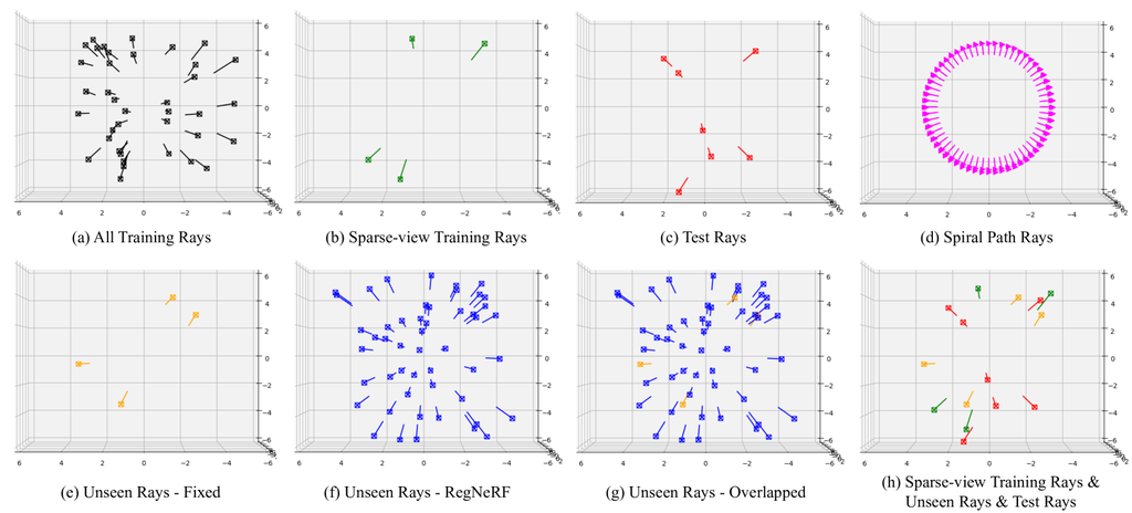
In Figure 12, we present the visualization of the sample space of the unseen rays from the RegNeRF [6] and our fixed unseen rays, which is used for fair comparison in the paper. Since they randomly sample the camera poses from the sample space in every training, we sample the $50$ unseen camera poses from the sample space to show the approximate coverage of the sample space. As we can see in the Figure 12, the fixed unseen rays, which are used in our experiments still in the coverage of the sample space of the RegNeRF. In addition, training camera poses and fixed unseen training rays do not significantly overlap with test rays, which also does not break the training and testing rule for novel view synthesis. Hence, it is not a problem to use the fixed unseen rays as alternative unseen rays of the RegNeRF. As we mentioned in Section V-C in the main paper, we utilize the fixed unseen rays for training our model to fairly evaluate the performances across the extensive experiments since the randomness of unseen ray generation in the RegNeRF makes it hard to understand the effectiveness of each component.

TABLE V: Image indices of each scene for training Sparse-DeRF.

Real Scene	Ball	Basket	Buick	Coffee	Decoration	Girl	Heron	Parterre	Puppet	Stair
$2$-view	1, 12	12, 33	11, 39	3, 10	1, 19	9, 16	11, 35	8, 26	9, 31	13, 26
$4$-view	1, 12, 18, 22	1, 12, 22, 33	5, 11, 20, 39	3, 10, 15, 26	1, 19, 22, 39	2, 9, 16, 32	4, 11, 18, 35	1, 8, 13, 26	9, 13, 21, 31	4, 13, 16, 26
$6$-view	1, 5, 10, 12, 18, 22	1, 8, 12, 17, 22, 33	5, 11, 17, 20, 34, 39	3, 10, 11, 15, 21, 26	1, 14, 19, 22, 27, 39	2, 9, 16, 24, 32, 37	4, 11, 18, 23, 27, 35	1, 8, 13, 17, 26, 28	7, 9, 13, 21, 23, 31	2, 4, 13, 16, 26, 34
Synthetic Scene	Cozyroom	Factory	Pool	Tanabata	Trolley
$2$-view	2, 17	3, 19	10, 23	1, 7	13, 23
$4$-view	2, 17, 23, 29	3, 14, 19, 33	5, 10, 15, 23	1, 7, 11, 22	7, 13, 23, 31
$6$-view	2, 14, 17, 21, 23, 29	1, 3, 14, 19, 28, 33	1, 5, 10, 15, 20, 23	1, 7, 11, 18, 22, 27	7, 13, 20, 23, 27, 31

TABLE VI: Hyper parameters of modulated gradient scaling (MGS) for entire scenes of the Deblur-NeRF [1] dataset. $\rho$ and $\eta$ denote the magnitude and period of sine function, respectively.

Synthetic Scene	Cozyroom	Factory	Pool	Tanabata	Trolley
$\rho$	10.0	10.0	10.0	1.0	10.0
$\eta$	1.75	1.75	1.75	1.5	1.75
Real Scene	Ball	Basket	Buick	Coffee	Decoration	Girl	Heron	Parterre	Puppet	Stair
$\rho$	1.0	1.0	10.0	1.0	1.0	1.0	1.0	1.0	10.0	1.0
$\eta$	1.2	0.67	1.75	0.67	0.5	0.5	0.5	0.5	1.75	0.5

Appendix B Additional Implementation Details

B-A Training Scene Indices

For fair comparison in future research, we present the image indices of each scene for training the Sparse-DeRF in TABLE V. The indices are manually selected from the training images of each scene as we mentioned in the main paper. Note that, the indices of the 2-view and 4-view settings are subsets of the 6-view setting.

B-B Parameters for Entire Scenes

In TABLE VI, we present the hyper-parameters of MGS for entire scenes, which consist of period $\eta$ and magnitude $\rho$ of the sine function. As we indicate in Section IV-B in the main paper, we set the magnitude $\rho$ as high value to only ignore the gradient in very near distance regions for scenes such as Buick, Puppet, Cozyroom, Factory, Pool, and Trolley. Please refer to the figure of the function shape depending on the parameters in the main paper.

Appendix C Additional Quantitative Results

C-A Quantitative Results for Entire Scenes

We present the comprehensive experimental results for entire scenes from 2-view, 4-view, and 6-view settings in TABLE VII, VIII, and IX, respectively. The results of the Sparse-DeRF in the TABLE VII, VIII, and IX are representative results as we presented in Section V-E1 in the main paper. In addition, we present more detailed ablation results for entire scenes from 2-view, 4-view, and 6-view settings in TABLE X, XI, and XII, respectively. As we mentioned before, we also present the separated ablation results according to the type of the kernel from DP-NeRF [2] and Deblur-NeRF [1].

C-B Complex Optimization Problem for Entire Scenes

We present the comprehensive experimental results of the complex optimization problem for entire scenes from 2-view, 4-view, and 6-view settings in TABLE XIV, XV, and XVI, respectively. In addition, we also present the quantitative results of the experiments on the Decoration scene that varies the number of sparse views in TABLE XIII as we mentioned in the main paper.

C-C Comparison to Naive Gradient Scaling for Entire Scenes

We present the quantitative comparison results for entire scenes that compare our modulated gradient scaling (MGS) and naive gradient scaling of [51] from 2-view, 4-view, and 6-view settings in TABLEXVII, XVIII, and XIX, respectively.

TABLE VII: Quantitative results of novel view synthesis for the entire scene of synthetic and real scenes obtained from 2-view settings. Each color shading represents the best, second best and third best result, respectively. DP-kernel and DN-kernel denote the kernel of [2] and [1].

Synthetic Scene	Factory			Cozyroom			Pool			Tanabata			Trolley			Average
	PSNR($\uparrow$)	SSIM($\uparrow$)	LPIPS($\downarrow$)	PSNR($\uparrow$)	SSIM($\uparrow$)	LPIPS($\downarrow$)	PSNR($\uparrow$)	SSIM($\uparrow$)	LPIPS($\downarrow$)	PSNR($\uparrow$)	SSIM($\uparrow$)	LPIPS($\downarrow$)	PSNR($\uparrow$)	SSIM($\uparrow$)	LPIPS($\downarrow$)	PSNR($\uparrow$)	SSIM($\uparrow$)	LPIPS($\downarrow$)
Naive NeRF [19]	14.24	.2186	.6867	21.07	.6127	.3644	18.59	.3575	.4288	10.84	.1517	.6500	10.82	.1591	.6593	15.11	.2999	.5578
MPR [56]+NeRF	14.43	.2250	.6858	21.08	.6111	.3671	18.72	.3676	.4228	11.03	.1456	.6553	10.56	.1535	.6663	15.16	.3006	.5595
Deblur-NeRF [1]	14.14	.2009	.6647	20.58	.5768	.3443	18.37	.3247	.4061	11.56	.1704	.6075	11.05	.1690	.6425	15.14	.2884	.5330
DP-NeRF [2]	14.14	.2091	.6540	20.71	.5752	.3487	18.38	.3276	.4127	11.21	.1482	.6247	10.88	.1536	.6543	15.06	.2827	.5389
RegNeRF [6] (No kernel)	14.57	.2523	.6680	17.13	.4616	.3808	14.23	.1473	.7298	13.01	.2408	.5956	14.04	.3227	.5602	14.60	.2849	.5869
RegNeRF [6] (w/DP-kernel)	14.20	.2214	.6412	18.88	.5136	.3476	13.03	.1003	.6845	9.21	.0815	.6920	10.86	.1644	.6657	13.24	.2162	.6062
Sparse-DeRF (w/DN-kernel) - Ours	14.27	.2200	.6564	20.57	.5675	.3589	19.81	.3330	.4058	11.67	.1827	.5947	11.28	.1800	.6298	15.52	.2966	.5291
Sparse-DeRF (w/DP-kernel) - Ours	14.10	.2116	.6413	18.97	.5206	.3417	20.32	.3488	.4056	12.00	.1943	.5902	11.36	.1769	.6422	15.35	.2904	.5242
Real Scene	Ball			Basket			Buick			Coffee			Decoration
	PSNR($\uparrow$)	SSIM($\uparrow$)	LPIPS($\downarrow$)	PSNR($\uparrow$)	SSIM($\uparrow$)	LPIPS($\downarrow$)	PSNR($\uparrow$)	SSIM($\uparrow$)	LPIPS($\downarrow$)	PSNR($\uparrow$)	SSIM($\uparrow$)	LPIPS($\downarrow$)	PSNR($\uparrow$)	SSIM($\uparrow$)	LPIPS($\downarrow$)
Naive NeRF [19]	18.45	.4363	.5693	13.32	.2595	.6131	13.49	.2620	.5680	17.76	.5249	.4807	12.25	.1718	.6738
MPR [56]+NeRF	18.69	.4413	.5659	13.09	.2505	.6194	13.31	.2574	.5706	18.13	.5243	.4869	12.41	.1761	.6735
Deblur-NeRF [1]	18.80	.4325	.5521	12.86	.2414	.5947	13.11	.2446	.5609	18.66	.5272	.4696	12.09	.1508	.6722
DP-NeRF [2]	18.22	.4200	.5611	13.24	.2263	.6062	13.43	.2480	.5571	18.15	.5191	.4876	12.34	.1672	.6675
RegNeRF [6] (No kernel)	20.48	.4951	.5398	15.53	.3388	.5403	17.05	.4241	.4361	23.24	.6950	.3505	10.94	.0816	.7545
RegNeRF [6] (w/DP-kernel)	18.58	.4297	.5565	13.49	.2429	.5985	12.51	.2199	.5579	15.71	.4280	.5370	11.15	.0927	.7520
Sparse-DeRF (w/DN-kernel) - Ours	20.07	.4612	.5290	13.62	.2678	.5835	14.38	.3182	.4913	19.51	.6048	.4146	13.09	.2173	.6256
Sparse-DeRF (w/DP-kernel) - Ours	20.09	.4583	.5244	14.05	.2890	.5555	13.78	.2864	.5036	19.67	.6084	.4096	13.11	.2192	.6192
Real Scene	Girl			Heron			Parterre			Puppet			Stair			Average
	PSNR($\uparrow$)	SSIM($\uparrow$)	LPIPS($\downarrow$)	PSNR($\uparrow$)	SSIM($\uparrow$)	LPIPS($\downarrow$)	PSNR($\uparrow$)	SSIM($\uparrow$)	LPIPS($\downarrow$)	PSNR($\uparrow$)	SSIM($\uparrow$)	LPIPS($\downarrow$)	PSNR($\uparrow$)	SSIM($\uparrow$)	LPIPS($\downarrow$)	PSNR($\uparrow$)	SSIM($\uparrow$)	LPIPS($\downarrow$)
Naive NeRF [19]	11.06	.2298	.6304	13.69	.1564	.5683	15.20	.2528	.6462	14.34	.2937	.6156	14.27	.0474	.6385	14.38	.2635	.6004
MPR [56]+NeRF	10.80	.1977	.6424	13.51	.1538	.5652	15.45	.2667	.6422	14.22	.2844	.6135	14.15	.0414	.6392	14.38	.2594	.6019
Deblur-NeRF [1]	10.94	.2031	.6436	13.97	.1459	.5499	15.02	.2320	.6431	14.28	.2764	.6036	14.40	.0525	.6313	14.41	.2506	.5921
DP-NeRF [2]	11.14	.2151	.6485	13.63	.1473	.5376	14.70	.2226	.6348	14.32	.2887	.5930	14.38	.0521	.6104	14.36	.2506	.5904
RegNeRF [6] (No kernel)	8.31	.0602	.7545	11.43	.0951	.6687	15.58	.2709	.6510	16.02	.3548	.5739	16.30	.1816	.6182	15.49	.2997	.5888
RegNeRF [6] (w/DP-kernel)	7.86	.0419	.7737	11.57	.0783	.6246	12.54	.1524	.7091	10.67	.1331	.6604	13.49	.0170	.6770	12.76	.1836	.6447
Sparse-DeRF (w/DN-kernel) - Ours	12.85	.3418	.5585	14.30	.1706	.5197	16.61	.2903	.5912	14.91	.3141	.5886	15.97	.1255	.6125	15.53	.3112	.5515
Sparse-DeRF (w/DP-kernel) - Ours	13.11	.3707	.5486	14.17	.1669	.5285	16.19	.2527	.5908	15.25	.3277	.5739	16.30	.1343	.6133	15.57	.3114	.5467

TABLE VIII: Quantitative results of novel view synthesis for the entire scenes of synthetic and real scenes obtained from 4-view settings. Each color shading represents the best, second best and third best result, respectively. DP-kernel and DN-kernel denote the kernel of [2] and [1].

Synthetic Scene	Factory			Cozyroom			Pool			Tanabata			Trolley			Average
	PSNR($\uparrow$)	SSIM($\uparrow$)	LPIPS($\downarrow$)	PSNR($\uparrow$)	SSIM($\uparrow$)	LPIPS($\downarrow$)	PSNR($\uparrow$)	SSIM($\uparrow$)	LPIPS($\downarrow$)	PSNR($\uparrow$)	SSIM($\uparrow$)	LPIPS($\downarrow$)	PSNR($\uparrow$)	SSIM($\uparrow$)	LPIPS($\downarrow$)	PSNR($\uparrow$)	SSIM($\uparrow$)	LPIPS($\downarrow$)
Naive NeRF [19]	16.63	.3494	.5861	22.75	.6935	.2903	25.92	.6419	.2495	16.15	.4408	.4635	18.66	.5380	.4104	20.02	.5327	.4000
MPR [56]+NeRF	16.97	.3570	.5789	22.86	.7014	.2895	25.77	.6436	.2465	16.78	.4827	.4361	17.61	.5056	.4272	20.00	.5381	.3956
Deblur-NeRF [1]	17.26	.3740	.5088	25.51	.7767	.1897	23.38	.5068	.2649	15.91	.4209	.4198	17.91	.5213	.3661	19.99	.5199	.3499
DP-NeRF [2]	19.20	.5175	.3813	21.50	.6242	.1980	21.85	.4235	.3117	17.30	.5265	.3381	19.35	.5765	.3084	19.84	.5336	.3075
RegNeRF [6] (No kernel)	16.32	.3441	.5876	23.25	.7155	.2663	16.21	.2040	.6451	17.35	.4915	.4509	18.81	.5447	.4020	18.39	.4600	.4704
RegNeRF [6] (w/DP-kernel)	16.71	.3497	.4683	21.37	.6471	.1802	15.17	.1740	.6666	10.27	.1165	.6911	18.66	.5412	.4067	16.44	.3657	.4826
Sparse-DeRF (w/DN-kernel) - Ours	16.91	.3693	.5357	25.79	.7872	.1801	25.48	.6042	.2405	16.58	.4705	.3793	18.10	.5514	.3414	20.57	.5565	.3354
Sparse-DeRF (w/DP-kernel) - Ours	18.99	.4770	.4034	26.51	.8051	.1627	23.33	.4888	.2733	17.51	.5371	.3356	18.92	.5799	.3126	21.05	.5776	.2975
Real Scene	Ball			Basket			Buick			Coffee			Decoration
	PSNR($\uparrow$)	SSIM($\uparrow$)	LPIPS($\downarrow$)	PSNR($\uparrow$)	SSIM($\uparrow$)	LPIPS($\downarrow$)	PSNR($\uparrow$)	SSIM($\uparrow$)	LPIPS($\downarrow$)	PSNR($\uparrow$)	SSIM($\uparrow$)	LPIPS($\downarrow$)	PSNR($\uparrow$)	SSIM($\uparrow$)	LPIPS($\downarrow$)
Naive NeRF [19]	21.61	.5043	.4992	17.23	fv.4384	.4746	19.20	.5508	.3579	23.21	.7341	.3281	14.78	.3299	.5640
MPR [56]+NeRF	21.46	.5046	.4992	16.98	.4260	.4766	19.39	.5486	.3629	22.98	.7267	.3284	14.88	.3460	.5532
Deblur-NeRF [1]	21.90	.5182	.4609	17.15	.4331	.4316	19.34	.5278	.3407	23.10	.7302	.2873	14.94	.3201	.5471
DP-NeRF [2]	23.20	.5842	.3847	17.42	.4046	.4658	19.26	.5323	.3374	24.05	.7597	.2624	14.98	.3018	.5618
RegNeRF [6] (No kernel)	21.16	.5100	.4952	18.12	.4711	.4569	20.11	.5821	.3412	26.14	.7837	.2965	11.35	.1045	.7030
RegNeRF [6] (w/DP-kernel)	19.13	.4391	.4042	17.42	.4165	.3746	13.31	.2697	.4715	16.40	.4684	.5239	11.07	.1058	.7089
Sparse-DeRF (w/DN-kernel) - Ours	22.28	.5506	.4334	18.69	.5058	.3774	19.28	.5414	.3371	26.76	.8126	.2419	17.12	.4192	.4761
Sparse-DeRF (w/DP-kernel) - Ours	23.39	.6010	.3806	20.41	.5451	.3305	19.48	.5531	.3251	27.77	.8364	.2049	16.33	.3914	.4950
Real Scene	Girl			Heron			Parterre			Puppet			Stair			Average
	PSNR($\uparrow$)	SSIM($\uparrow$)	LPIPS($\downarrow$)	PSNR($\uparrow$)	SSIM($\uparrow$)	LPIPS($\downarrow$)	PSNR($\uparrow$)	SSIM($\uparrow$)	LPIPS($\downarrow$)	PSNR($\uparrow$)	SSIM($\uparrow$)	LPIPS($\downarrow$)	PSNR($\uparrow$)	SSIM($\uparrow$)	LPIPS($\downarrow$)	PSNR($\uparrow$)	SSIM($\uparrow$)	LPIPS($\downarrow$)
Naive NeRF [19]	15.91	.5659	.4161	18.83	.4263	.4086	20.64	.4857	.4822	18.15	.4619	.4470	20.27	.3622	.5033	18.98	.4860	.4481
MPR [56]+NeRF	15.60	.5617	.4224	18.91	.4217	.4173	20.76	.4893	.4781	17.96	.4548	.4468	19.94	.3493	.4993	18.89	.4829	.4484
Deblur-NeRF [1]	15.62	.5351	.4206	18.85	.4350	.3398	19.71	.4318	.4549	17.77	.4400	.4358	20.49	.3901	.4326	18.89	.4761	.4151
DP-NeRF [2]	15.40	.5237	.4318	18.68	.4292	.3352	17.62	.2987	.4991	17.61	.4369	.4313	19.44	.3107	.4657	18.77	.4582	.4175
RegNeRF [6] (No kernel)	10.24	.1511	.7199	18.86	.4235	.4194	18.68	.4238	.5163	18.66	.4788	.4327	21.06	.3975	.4706	18.44	.4326	.4852
RegNeRF [6] (w/DP-kernel)	9.52	.1304	.7119	11.56	.0595	.6149	13.61	.1721	.7245	11.10	.1342	.6914	12.73	.0249	.6610	13.59	.2221	.5887
Sparse-DeRF (w/DN-kernel) - Ours	16.95	.5975	.3823	19.04	.4558	.3315	20.74	.4916	.4323	18.11	.4616	.4202	20.80	.3948	.4386	19.98	.5231	.3871
Sparse-DeRF (w/DP-kernel) - Ours	16.47	.5855	.3835	19.09	.4624	.3194	18.36	.3375	.4715	17.97	.4612	.4206	21.25	.4045	.4044	20.05	.5178	.3736

TABLE IX: Quantitative results of novel view synthesis for the entire scenes of synthetic and real scenes obtained from 6-view settings. Each color shading represents the best, second best and third best result, respectively. DP-kernel and DN-kernel denote the kernel of [2] and [1].

Synthetic Scene	Factory			Cozyroom			Pool			Tanabata			Trolley			Average
	PSNR($\uparrow$)	SSIM($\uparrow$)	LPIPS($\downarrow$)	PSNR($\uparrow$)	SSIM($\uparrow$)	LPIPS($\downarrow$)	PSNR($\uparrow$)	SSIM($\uparrow$)	LPIPS($\downarrow$)	PSNR($\uparrow$)	SSIM($\uparrow$)	LPIPS($\downarrow$)	PSNR($\uparrow$)	SSIM($\uparrow$)	LPIPS($\downarrow$)	PSNR($\uparrow$)	SSIM($\uparrow$)	LPIPS($\downarrow$)
Naive NeRF [19]	17.12	.3663	.5663	23.12	.7160	.2713	28.42	.7463	.2106	19.92	.5889	.3866	19.68	.5749	.3853	21.65	.5985	.3638
MPR [56]+NeRF	17.21	.3754	.5649	23.06	.7087	.2749	28.38	.7461	.2093	20.23	.5966	.3783	19.71	.5728	.3870	21.72	.5999	.3629
Deblur-NeRF [1]	18.77	.5048	.3890	26.67	.8214	.1475	27.50	.7116	.1783	21.10	.6693	.2517	21.58	.6921	.2263	23.12	.6798	.2386
DP-NeRF [2]	21.63	.6402	.2984	27.63	.8475	.1224	25.36	.6227	.1861	21.27	.6818	.2023	22.49	.7259	.1899	23.68	.7036	.1998
RegNeRF [6] (No kernel)	17.04	.3690	.5729	23.40	.7205	.2649	18.05	.3610	.4870	20.33	.5980	.3745	19.63	.5760	.3833	19.69	.5249	.4165
RegNeRF [6] (w/DP-kernel)	21.03	.6273	.3076	27.73	.8455	.1238	18.04	.3173	.4987	21.84	.7246	.2022	19.36	.5661	.3908	21.60	.6162	.3046
Sparse-DeRF (w/DN-kernel) - Ours	18.33	.5144	.4004	26.63	.8184	.1513	28.16	.7344	.1755	22.06	.6988	.2245	21.43	.6855	.2380	23.32	.6903	.2379
Sparse-DeRF (w/DP-kernel) - Ours	21.29	.6179	.3261	27.34	.8340	.1298	28.19	.7365	.1606	22.30	.7233	.2017	22.21	.7159	.2036	24.27	.7255	.2044
Real Scene	Ball			Basket			Buick			Coffee			Decoration
	PSNR($\uparrow$)	SSIM($\uparrow$)	LPIPS($\downarrow$)	PSNR($\uparrow$)	SSIM($\uparrow$)	LPIPS($\downarrow$)	PSNR($\uparrow$)	SSIM($\uparrow$)	LPIPS($\downarrow$)	PSNR($\uparrow$)	SSIM($\uparrow$)	LPIPS($\downarrow$)	PSNR($\uparrow$)	SSIM($\uparrow$)	LPIPS($\downarrow$)
Naive NeRF [19]	22.12	.5359	.4818	21.39	.6253	.3328	21.21	.6197	.3100	22.73	.7163	.3397	19.14	.5118	.4460
MPR [56]+NeRF	22.15	.5365	.4745	21.39	.6261	.3294	21.11	.6192	.3063	22.56	.7087	.3435	18.31	.4837	.4735
Deblur-NeRF [1]	24.47	.6473	.3342	23.63	.7204	.2108	21.45	.6285	.2625	23.70	.7604	.2588	17.74	.4790	.4296
DP-NeRF [2]	24.73	.6651	.3107	23.24	.6643	.2494	21.65	.6418	.2445	25.51	.7949	.2170	17.48	.4725	.4457
RegNeRF [6] (No kernel)	21.98	.5312	.4677	21.67	.6129	.3406	21.16	.6215	.3051	25.67	.7716	.3105	12.45	.1569	.7061
RegNeRF [6] (w/DP-kernel)	25.02	.6719	.2953	22.95	.6554	.2501	21.57	.6456	.2462	23.38	.7393	.2341	11.43	.1247	.6932
Sparse-DeRF (w/DN-kernel) - Ours	23.76	.6184	.3607	23.39	.7155	.2329	21.66	.6405	.2585	27.84	.8388	.2068	19.98	.5553	.3644
Sparse-DeRF (w/DP-kernel) - Ours	24.80	.6643	.3200	23.32	.6789	.2455	21.27	.6234	.2662	28.91	.8525	.1902	19.69	.5440	.3672
Real Scene	Girl			Heron			Parterre			Puppet			Stair			Average
	PSNR($\uparrow$)	SSIM($\uparrow$)	LPIPS($\downarrow$)	PSNR($\uparrow$)	SSIM($\uparrow$)	LPIPS($\downarrow$)	PSNR($\uparrow$)	SSIM($\uparrow$)	LPIPS($\downarrow$)	PSNR($\uparrow$)	SSIM($\uparrow$)	LPIPS($\downarrow$)	PSNR($\uparrow$)	SSIM($\uparrow$)	LPIPS($\downarrow$)	PSNR($\uparrow$)	SSIM($\uparrow$)	LPIPS($\downarrow$)
Naive NeRF [19]	18.43	.6500	.3335	18.91	.4204	.4307	21.82	.5487	.4351	19.52	.5242	.3933	21.01	.3602	.5111	20.63	.5513	.4014
MPR [56]+NeRF	18.61	.6580	.3324	18.97	.4220	.4287	21.78	.5477	.4358	19.84	.5357	.3793	21.27	.3758	.4070	20.60	.5513	.4010
Deblur-NeRF [1]	18.09	.6582	.3055	19.40	.4709	.3166	21.92	.5557	.3872	20.58	.5834	.3226	22.60	.4993	.3349	21.36	.6003	.3163
DP-NeRF [2]	18.16	.6622	.3020	19.58	.4991	.2905	22.36	.5879	.3350	20.65	.5868	.2988	23.40	.5624	.2986	21.68	.6137	.2992
RegNeRF [6] (No kernel)	11.06	.1966	.7091	18.96	.4218	.4292	21.83	.5526	.4353	20.07	.5309	.3827	21.69	.3938	.4963	19.65	.4790	.4583
RegNeRF [6] (w/DP-kernel)	10.38	.1434	.7200	12.83	.1019	.5757	21.34	.5159	.3415	20.49	.5799	.3113	13.08	.2613	.6581	18.25	.4439	.4326
Sparse-DeRF (w/DN-kernel) - Ours	18.86	.6860	.2769	19.63	.5011	.2992	22.15	.5703	.3787	20.81	.5882	.3149	23.42	.5340	.3374	22.15	.6248	.3030
Sparse-DeRF (w/DP-kernel) - Ours	18.96	.6887	.2744	19.59	.5051	.2808	22.57	.5994	.3317	20.60	.5756	.3124	23.48	.5509	.3189	22.32	.6283	.2907

TABLE X: Ablation quantitative results of novel view synthesis for the entire scenes of synthetic and real scenes obtained from 2-view settings. Each color shading represents the best, second best and third best result, respectively. DP-kernel and DN-kernel denote the kernel of [2] and [1].

Kernel Type	Synthetic Scene			Factory			Cozyroom			Pool			Tanabata			Trolley			Average
	SS	MGS	PD	PSNR($\uparrow$)	SSIM($\uparrow$)	LPIPS($\downarrow$)	PSNR($\uparrow$)	SSIM($\uparrow$)	LPIPS($\downarrow$)	PSNR($\uparrow$)	SSIM($\uparrow$)	LPIPS($\downarrow$)	PSNR($\uparrow$)	SSIM($\uparrow$)	LPIPS($\downarrow$)	PSNR($\uparrow$)	SSIM($\uparrow$)	LPIPS($\downarrow$)	PSNR($\uparrow$)	SSIM($\uparrow$)	LPIPS($\downarrow$)
DP-kernel				14.14	.2091	.6540	20.71	.5752	.3487	18.38	.3276	.4127	11.21	.1482	.6247	10.88	.1536	.6543	15.06	.2827	.5389
	✓			14.09	.2008	.6550	19.57	.5321	.3544	18.49	.3178	.4271	11.21	.1552	.6243	11.04	.1801	.6331	14.88	.2772	.5388
		✓		14.33	.2088	.6496	18.89	.5032	.3577	20.30	.3467	.4017	11.69	.1748	.6067	11.78	.1948	.6289	15.40	.2857	.5289
			✓	14.19	.2035	.6620	19.82	.5404	.3451	18.96	.3350	.4125	11.16	.1457	.6408	11.02	.1733	.6350	15.03	.2796	.5391
	✓		✓	13.95	.1963	.6629	18.81	.5010	.3637	18.57	.3404	.4148	11.00	.1501	.6259	10.25	.1357	.6730	14.52	.2647	.5481
	✓	✓		14.24	.2228	.6439	20.16	.5560	.3391	20.37	.3526	.4004	11.55	.1710	.5999	11.16	.1744	.6241	15.50	.2954	.5215
	✓	✓	✓	14.10	.2116	.6413	18.97	.5206	.3417	20.32	.3488	.4056	12.00	.1943	.5902	11.36	.1769	.6422	15.35	.2904	.5242
DN-kernel				14.14	.2009	.6647	20.58	.5768	.3443	18.37	.3247	.4061	11.56	.1704	.6075	11.05	.1690	.6425	15.14	.2884	.5330
	✓			14.21	.2177	.6650	20.33	.5663	.3591	18.74	.3200	.4093	11.13	.1547	.6191	10.78	.1554	.6566	15.04	.2828	.5418
		✓		14.20	.2107	.6686	21.02	.5999	.3326	19.64	.3330	.3950	11.55	.1804	.5903	11.48	.1883	.6351	15.12	.3025	.5243
			✓	14.11	.2096	.6588	18.78	.5094	.3928	19.76	.3464	.3901	10.58	.1206	.6565	10.99	.1648	.6289	14.84	.2702	.5454
	✓		✓	14.24	.2222	.6619	21.02	.5918	.3544	18.77	.3197	.4115	11.12	.1642	.6217	10.41	.1467	.6452	15.11	.2889	.5389
	✓	✓		14.14	.2189	.6622	20.10	.5555	.3761	20.11	.3372	.3939	11.49	.1753	.5975	11.99	.2026	.6299	15.57	.2979	.5319
	✓	✓	✓	14.27	.2200	.6564	20.57	.5675	.3589	19.81	.3330	.4058	11.67	.1827	.5947	11.28	.1800	.6298	15.52	.2966	.5291
	Real Scene			Ball			Basket			Buick			Coffee			Decoration
	SS	MGS	PD	PSNR($\uparrow$)	SSIM($\uparrow$)	LPIPS($\downarrow$)	PSNR($\uparrow$)	SSIM($\uparrow$)	LPIPS($\downarrow$)	PSNR($\uparrow$)	SSIM($\uparrow$)	LPIPS($\downarrow$)	PSNR($\uparrow$)	SSIM($\uparrow$)	LPIPS($\downarrow$)	PSNR($\uparrow$)	SSIM($\uparrow$)	LPIPS($\downarrow$)
DP-kernel				18.22	.4200	.5611	13.24	.2263	.6062	13.43	.2480	.5571	18.15	.5191	.4876	12.34	.1672	.6675
	✓			18.76	.4329	.5521	12.68	.2189	.6301	13.05	.2269	.5657	17.51	.4792	.4907	12.28	.1638	.6619
		✓		19.80	.4544	.5273	14.08	.2706	.5509	13.96	.3028	.4992	19.72	.6115	.4035	13.14	.2198	.6201
			✓	18.28	.4191	.5591	12.95	.2281	.5951	13.49	.2654	.5464	17.92	.5030	.4875	12.04	.1491	.6700
	✓		✓	18.50	.4341	.5537	12.92	.2407	.5938	13.64	.2564	.5427	18.09	.5263	.4689	12.42	.1669	.6689
	✓	✓		19.80	.4412	.5346	14.28	.2913	.5520	13.82	.2920	.5013	18.81	.5712	.4363	13.04	.2166	.6203
	✓	✓	✓	20.09	.4583	.5244	14.05	.2890	.5555	13.78	.2864	.5036	19.67	.6084	.4096	13.11	.2192	.6192
DN-kernel				18.80	.4325	.5521	12.86	.2414	.5947	13.11	.2446	.5609	18.66	.5272	.4696	12.09	.1508	.6722
	✓			18.88	.4388	.5519	13.03	.2516	.6018	13.36	.2533	.5523	18.04	.5145	.4847	12.38	.1736	.6545
		✓		19.95	.4596	.5394	13.52	.2534	.5871	14.11	.3087	.5051	19.33	.6003	.4133	13.13	.2153	.6222
			✓	18.70	.4235	.5673	13.24	.2505	.5931	13.52	.2520	.5438	18.15	.5031	.4949	12.32	.1683	.6617
	✓		✓	18.36	.4140	.5667	13.14	.2482	.5975	13.40	.2549	.5461	17.90	.5098	.4857	12.37	.1634	.6658
	✓	✓		20.06	.4637	.5299	13.56	.2593	.5828	14.51	.3204	.4869	19.40	.5956	.4198	13.07	.2189	.6230
	✓	✓	✓	20.07	.4612	.5290	13.62	.2678	.5835	14.38	.3182	.4913	19.51	.6048	.4146	13.09	.2173	.6256
	Real Scene			Girl			Heron			Parterre			Puppet			Stair			Average
	SS	MGS	PD	PSNR($\uparrow$)	SSIM($\uparrow$)	LPIPS($\downarrow$)	PSNR($\uparrow$)	SSIM($\uparrow$)	LPIPS($\downarrow$)	PSNR($\uparrow$)	SSIM($\uparrow$)	LPIPS($\downarrow$)	PSNR($\uparrow$)	SSIM($\uparrow$)	LPIPS($\downarrow$)	PSNR($\uparrow$)	SSIM($\uparrow$)	LPIPS($\downarrow$)	PSNR($\uparrow$)	SSIM($\uparrow$)	LPIPS($\downarrow$)
DP-kernel				11.14	.2151	.6485	13.63	.1473	.5376	14.70	.2226	.6348	14.32	.2887	.5930	14.38	.0521	.6104	14.36	.2506	.5904
	✓			10.75	.1816	.6600	14.05	.1553	.5467	15.17	.2340	.6205	14.13	.2770	.5934	14.24	.0442	.6120	14.26	.2414	.5933
		✓		12.89	.3465	.5645	14.48	.1677	.5209	16.20	.2511	.5927	14.48	.2941	.5819	15.81	.1167	.6039	15.46	.3035	.5465
			✓	11.09	.2039	.6398	13.52	.1381	.5553	14.73	.2355	.6403	14.37	.2918	.5857	14.49	.0555	.6165	14.28	.2490	.5896
	✓		✓	11.19	.2311	.6275	13.86	.1524	.5365	15.44	.2498	.6124	14.03	.2771	.6020	14.40	.0518	.6231	14.00	.2587	.5830
	✓	✓		12.78	.3357	.5685	14.45	.1741	.5228	16.36	.2643	.5939	14.56	.2958	.5918	16.11	.1267	.6054	15.40	.3009	.5527
	✓	✓	✓	13.11	.3707	.5486	14.17	.1669	.5285	16.19	.2527	.5908	15.25	.3277	.5739	16.30	.1343	.6133	15.57	.3114	.5467
DN-kernel				10.94	.2031	.6436	13.97	.1459	.5499	15.02	.2320	.6431	14.28	.2764	.6036	14.40	.0525	.6313	14.41	.2506	.5921
	✓			10.43	.1696	.6654	13.10	.1336	.5652	15.09	.2075	.6536	14.66	.3000	.5950	14.36	.0528	.6122	14.33	.2495	.5937
		✓		12.55	.3184	.5736	14.51	.1850	.5217	16.65	.2830	.5953	14.68	.2944	.5924	15.93	.1189	.6081	15.44	.3037	.5558
			✓	11.19	.2214	.6475	13.95	.1421	.5508	14.30	.2189	.6739	14.99	.3117	.5894	14.35	.0574	.6164	14.47	.2549	.5939
	✓		✓	11.55	.2299	.6195	13.93	.1543	.5382	14.92	.2291	.6399	14.74	.3042	.6001	14.43	.0556	.6211	14.47	.2563	.5881
	✓	✓		12.70	.3438	.5627	14.57	.1779	.5200	16.51	.2872	.5825	14.24	.2848	.6097	16.02	.1216	.6018	15.46	.3073	.5519
	✓	✓	✓	12.85	.3418	.5585	14.30	.1706	.5197	16.61	.2903	.5912	14.91	.3141	.5886	15.97	.1255	.6125	15.53	.3112	.5515

TABLE XI: Ablation quantitative results of novel view synthesis for the entire scenes of synthetic and real scenes obtained from 4-view settings. Each color shading represents the best, second best and third best result, respectively. DP-kernel and DN-kernel denote the kernel of [2] and [1].

Kernel Type	Synthetic Scene			Factory			Cozyroom			Pool			Tanabata			Trolley			Average
	SS	MGS	PD	PSNR($\uparrow$)	SSIM($\uparrow$)	LPIPS($\downarrow$)	PSNR($\uparrow$)	SSIM($\uparrow$)	LPIPS($\downarrow$)	PSNR($\uparrow$)	SSIM($\uparrow$)	LPIPS($\downarrow$)	PSNR($\uparrow$)	SSIM($\uparrow$)	LPIPS($\downarrow$)	PSNR($\uparrow$)	SSIM($\uparrow$)	LPIPS($\downarrow$)	PSNR($\uparrow$)	SSIM($\uparrow$)	LPIPS($\downarrow$)
DP-kernel				19.20	.5175	.3813	21.50	.6242	.1980	21.85	.4235	.3117	17.30	.5265	.3381	19.35	.5765	.3084	19.84	.5336	.3075
	✓			19.01	.4914	.4082	21.69	.6356	.1889	22.62	.4520	.3013	16.61	.4789	.3771	17.82	.5385	.3475	19.55	.5193	.3246
		✓		18.22	.4638	.4144	22.48	.6603	.1762	23.11	.4709	.2791	18.18	.5517	.3124	18.83	.5657	.3299	20.16	.5425	.3024
			✓	18.79	.4972	.3974	22.59	.6760	.2314	22.41	.4348	.3011	16.88	.4913	.3606	17.59	.5194	.3652	19.65	.5237	.3311
	✓		✓	19.09	.5253	.3889	25.83	.7796	.1709	24.13	.5229	.2474	16.95	.5017	.3501	18.56	.5764	.3167	20.91	.5812	.2948
	✓	✓		17.62	.4227	.4615	23.43	.7266	.1688	22.71	.4454	.2850	15.64	.4150	.4308	18.84	.5722	.3209	19.65	.5164	.3334
	✓	✓	✓	18.99	.4770	.4034	26.51	.8051	.1627	23.33	.4888	.2733	17.51	.5371	.3356	18.92	.5799	.3126	21.05	.5776	.2975
DN-kernel				17.26	.3740	.5088	25.51	.7767	.1897	23.38	.5068	.2649	15.91	.4209	.4198	17.91	.5213	.3661	19.99	.5199	.3499
	✓			16.89	.3611	.5353	25.82	.7876	.1770	22.92	.4820	.2809	15.52	.4381	.4173	18.07	.5317	.3684	19.89	.5201	.3558
		✓		16.33	.3387	.5636	25.55	.7813	.1874	24.28	.5544	.2649	16.60	.4635	.3781	17.96	.5095	.3870	19.44	.5295	.3562
			✓	16.49	.3444	.5691	25.40	.7674	.1982	21.87	.4194	.3203	16.48	.4798	.3830	18.38	.5412	.3445	19.72	.5104	.3630
	✓		✓	17.11	.3766	.5195	25.43	.7770	.1891	22.41	.4585	.2864	16.63	.4792	.3826	18.57	.5559	.3476	20.03	.5294	.3450
	✓	✓		16.22	.3389	.5637	25.12	.7566	.1950	23.00	.4792	.2810	17.37	.5088	.3661	18.08	.5275	.3677	19.96	.5222	.3547
	✓	✓	✓	16.91	.3693	.5357	25.79	.7872	.1801	25.48	.6042	.2405	16.58	.4705	.3793	18.10	.5514	.3414	20.57	.5565	.3354
	Real Scene			Ball			Basket			Buick			Coffee			Decoration
	SS	MGS	PD	PSNR($\uparrow$)	SSIM($\uparrow$)	LPIPS($\downarrow$)	PSNR($\uparrow$)	SSIM($\uparrow$)	LPIPS($\downarrow$)	PSNR($\uparrow$)	SSIM($\uparrow$)	LPIPS($\downarrow$)	PSNR($\uparrow$)	SSIM($\uparrow$)	LPIPS($\downarrow$)	PSNR($\uparrow$)	SSIM($\uparrow$)	LPIPS($\downarrow$)
DP-kernel				23.20	.5842	.3847	17.42	.4046	.4658	19.26	.5323	.3374	24.05	.7597	.2624	14.98	.3018	.5618
	✓			23.55	.6053	.3685	18.32	.4442	.4292	19.35	.5340	.3339	23.17	.7442	.2670	16.14	.3739	.5082
		✓		22.52	.5522	.3689	20.31	.5388	.3364	19.16	.5203	.3430	25.62	.7884	.2082	17.33	.4081	.4777
			✓	23.18	.5817	.3878	17.63	.4194	.4475	19.53	.5441	.3325	24.85	.7885	.2467	14.99	.3407	.5267
	✓		✓	23.30	.5893	.3904	18.49	.4615	.3926	19.14	.5385	.3408	24.05	.7716	.2494	15.25	.3458	.5274
	✓	✓		22.36	.5504	.3612	19.61	.5134	.3661	19.27	.5458	.3316	27.55	.8167	.2242	16.53	.3902	.4867
	✓	✓	✓	23.39	.6010	.3806	20.41	.5451	.3305	19.48	.5531	.3251	27.77	.8364	.2049	16.33	.3914	.4950
DN-kernel				21.90	.5182	.4609	17.15	.4331	.4316	19.34	.5278	.3407	23.10	.7302	.2873	14.94	.3201	.5471
	✓			21.94	.5220	.4571	17.38	.4464	.4298	19.26	.5401	.3418	23.03	.7264	.2830	14.82	.3293	.5363
		✓		21.85	.5168	.4514	17.87	.4641	.4014	19.23	.5289	.3467	26.91	.8082	.2473	16.69	.4031	.4859
			✓	21.85	.5313	.4392	16.97	.4301	.4228	19.45	.5443	.3403	23.78	.7679	.2754	15.18	.3549	.5112
	✓		✓	22.06	.5319	.4481	16.75	.4308	.4333	19.34	.5421	.3373	23.44	.7421	.2943	14.86	.3429	.5299
	✓	✓		22.09	.5299	.4477	17.81	.4854	.3812	19.31	.5400	.3384	27.40	.8263	.2353	16.93	.4023	.4879
	✓	✓	✓	22.28	.5506	.4334	18.69	.5058	.3774	19.28	.5414	.3371	26.76	.8126	.2419	17.12	.4192	.4761
	Real Scene			Girl			Heron			Parterre			Puppet			Stair			Average
	SS	MGS	PD	PSNR($\uparrow$)	SSIM($\uparrow$)	LPIPS($\downarrow$)	PSNR($\uparrow$)	SSIM($\uparrow$)	LPIPS($\downarrow$)	PSNR($\uparrow$)	SSIM($\uparrow$)	LPIPS($\downarrow$)	PSNR($\uparrow$)	SSIM($\uparrow$)	LPIPS($\downarrow$)	PSNR($\uparrow$)	SSIM($\uparrow$)	LPIPS($\downarrow$)	PSNR($\uparrow$)	SSIM($\uparrow$)	LPIPS($\downarrow$)
DP-kernel				15.40	.5237	.4318	18.68	.4292	.3352	17.62	.2987	.4991	17.61	.4369	.4313	19.44	.3107	.4657	18.77	.4582	.4175
	✓			15.67	.5342	.4274	18.44	.4145	.3322	17.37	.2900	.4935	18.49	.4765	.3982	19.85	.3433	.4503	19.04	.4760	.4008
		✓		17.03	.6045	.3636	18.90	.4526	.3185	18.38	.3323	.4575	17.89	.4408	.4333	20.33	.3416	.4297	19.75	.4980	.3737
			✓	14.80	.4950	.4538	18.83	.4336	.3308	17.81	.3089	.4915	18.12	.4505	.4205	20.23	.3615	.4422	19.00	.4724	.4080
	✓		✓	15.57	.5297	.4349	19.04	.4578	.3278	17.88	.3094	.4887	17.84	.4461	.4329	19.47	.3102	.4522	19.00	.4760	.4037
	✓	✓		16.78	.5919	.3806	18.99	.4575	.3166	18.28	.3333	.4630	17.63	.4272	.4243	20.36	.3594	.4201	19.74	.4986	.3774
	✓	✓	✓	16.47	.5855	.3835	19.09	.4624	.3194	18.36	.3375	.4715	17.97	.4612	.4206	21.25	.4045	.4044	20.05	.5178	.3736
DN-kernel				15.62	.5351	.4206	18.85	.4350	.3398	19.71	.4318	.4549	17.77	.4400	.4358	20.49	.3901	.4326	18.89	.4761	.4151
	✓			15.04	.5147	.4312	18.75	.4291	.3585	20.73	.4841	.4379	18.15	.4647	.4248	20.45	.3825	.4249	18.96	.4839	.4125
		✓		17.13	.6103	.3623	18.96	.4527	.3366	20.47	.4735	.4464	18.39	.4694	.4156	20.94	.3914	.4432	19.84	.5118	.3937
			✓	15.17	.5215	.4383	18.97	.4367	.3480	20.57	.4833	.4463	18.24	.4620	.4252	20.42	.3752	.4578	19.06	.4907	.4105
	✓		✓	15.48	.5272	.4282	19.00	.4430	.3458	20.37	.4801	.4401	18.08	.4577	.4276	20.05	.3635	.4601	18.94	.4861	.4145
	✓	✓		17.07	.6081	.3706	18.95	.4514	.3254	20.64	.4854	.4385	18.03	.4510	.4298	21.05	.4086	.4182	19.93	.5188	.3873
	✓	✓	✓	16.95	.5975	.3823	19.04	.4558	.3315	20.74	.4916	.4323	18.11	.4616	.4202	20.80	.3948	.4386	19.98	.5231	.3871

TABLE XII: Ablation quantitative results of novel view synthesis for the entire scenes of synthetic and real scenes obtained from 6-view settings. Each color shading represents the best, second best and third best result, respectively. DP-kernel and DN-kernel denote the kernel of [2] and [1].

Kernel Type	Synthetic Scene			Factory			Cozyroom			Pool			Tanabata			Trolley			Average
	SS	MGS	PD	PSNR($\uparrow$)	SSIM($\uparrow$)	LPIPS($\downarrow$)	PSNR($\uparrow$)	SSIM($\uparrow$)	LPIPS($\downarrow$)	PSNR($\uparrow$)	SSIM($\uparrow$)	LPIPS($\downarrow$)	PSNR($\uparrow$)	SSIM($\uparrow$)	LPIPS($\downarrow$)	PSNR($\uparrow$)	SSIM($\uparrow$)	LPIPS($\downarrow$)	PSNR($\uparrow$)	SSIM($\uparrow$)	LPIPS($\downarrow$)
DP-kernel				21.63	.6402	.2984	27.63	.8475	.1224	25.36	.6227	.1861	21.27	.6818	.2023	22.49	.7259	.1899	23.68	.7036	.1998
	✓			21.84	.6556	.2947	27.48	.8419	.1272	26.73	.6891	.1687	22.57	.7289	.1950	22.15	.7160	.2015	24.15	.7263	.1974
		✓		19.30	.5628	.3553	27.56	.8408	.1262	28.10	.7374	.1544	21.83	.7128	.2074	22.34	.7197	.1928	23.83	.7147	.2072
			✓	20.52	.5994	.3224	27.29	.8322	.1349	27.07	.7002	.1719	22.50	.7306	.1958	22.07	.7127	.2011	23.89	.7150	.2052
	✓		✓	21.27	.6104	.3191	27.39	.8376	.1301	28.54	.7518	.1608	22.32	.7290	.1966	21.87	.7109	.2037	24.28	.7279	.2021
	✓	✓		18.43	.5407	.3738	27.44	.8399	.1313	27.89	.7321	.1596	22.02	.7197	.2071	21.87	.7118	.2046	23.53	.7088	.2153
	✓	✓	✓	21.29	.6179	.3261	27.34	.8340	.1298	28.19	.7365	.1606	22.30	.7233	.2017	22.21	.7159	.2036	24.27	.7255	.2044
DN-kernel				18.77	.5048	.3890	26.67	.8214	.1475	27.50	.7116	.1783	21.10	.6693	.2517	21.58	.6921	.2263	23.12	.6798	.2386
	✓			17.87	.4554	.4370	26.76	.8239	.1462	28.12	.7316	.1735	21.69	.6979	.2282	21.61	.6887	.2294	23.59	.6795	.2429
		✓		18.06	.4849	.4104	26.54	.8159	.1486	28.09	.7392	.1725	20.97	.6866	.2394	21.71	.6895	.2320	24.33	.6832	.2406
			✓	19.22	.5397	.3756	26.52	.8184	.1514	27.72	.7242	.1828	21.67	.6961	.2306	21.64	.6920	.2300	23.35	.6941	.2341
	✓		✓	19.77	.5461	.3692	26.63	.8192	.1480	28.17	.7353	.1733	21.08	.6878	.2367	21.39	.6821	.2347	23.41	.6941	.2324
	✓	✓		17.50	.4349	.4613	26.72	.8226	.1491	27.40	.7046	.1848	21.73	.6962	.2369	21.20	.6688	.2477	22.91	.6654	.2560
	✓	✓	✓	18.33	.5144	.4004	26.63	.8184	.1513	28.16	.7344	.1755	22.06	.6988	.2245	21.43	.6855	.2380	23.32	.6903	.2379
	Real Scene			Ball			Basket			Buick			Coffee			Decoration
	SS	MGS	PD	PSNR($\uparrow$)	SSIM($\uparrow$)	LPIPS($\downarrow$)	PSNR($\uparrow$)	SSIM($\uparrow$)	LPIPS($\downarrow$)	PSNR($\uparrow$)	SSIM($\uparrow$)	LPIPS($\downarrow$)	PSNR($\uparrow$)	SSIM($\uparrow$)	LPIPS($\downarrow$)	PSNR($\uparrow$)	SSIM($\uparrow$)	LPIPS($\downarrow$)
DP-kernel				24.73	.6651	.3107	23.24	.6643	.2494	21.65	.6418	.2445	25.52	.7949	.2170	17.48	.4725	.4457
	✓			24.93	.6697	.3054	22.91	.6688	.2453	21.48	.6400	.2580	28.12	.8224	.1987	18.34	.4934	.4226
		✓		24.21	.6412	.3094	22.82	.6631	.2508	21.17	.6251	.2681	28.39	.8448	.1722	19.82	.5485	.3697
			✓	24.92	.6661	.3111	22.27	.6326	.2860	21.30	.6234	.2710	26.62	.7973	.2259	18.07	.4926	.4230
	✓		✓	24.86	.6598	.3181	21.29	.6094	.3065	21.40	.6359	.2584	28.58	.8332	.1910	17.78	.4869	.4352
	✓	✓		25.01	.6691	.3007	23.19	.6706	.2481	21.12	.6212	.2662	28.23	.8410	.1798	19.88	.5550	.3606
	✓	✓	✓	24.80	.6643	.3200	23.32	.6789	.2455	21.27	.6234	.2662	28.91	.8525	.1902	19.69	.5440	.3672
DN-kernel				24.47	.6473	.3342	23.63	.7204	.2108	21.45	.6285	.2625	23.70	.7604	.2588	17.74	.4790	.4296
	✓			23.02	.5757	.3964	22.96	.7128	.2230	21.72	.6389	.2595	26.90	.8004	.2354	17.21	.4774	.4346
		✓		24.15	.6343	.3465	22.59	.6894	.2365	21.30	.6185	.2678	26.41	.7947	.2300	19.38	.5272	.3908
			✓	23.68	.6175	.3572	22.90	.7035	.2255	20.95	.6172	.2716	27.18	.8083	2336	18.53	.5030	.4084
	✓		✓	24.60	.6530	.3439	22.96	.7132	.2296	21.43	.6360	.2642	26.13	.8178	.2159	18.07	.4784	.4420
	✓	✓		23.93	.6332	.3464	23.89	.7342	.2188	21.11	.6247	.2747	26.88	.8074	.2403	19.53	.5383	.3855
	✓	✓	✓	23.76	.6184	.3607	23.39	.7155	.2329	21.66	.6405	.2585	27.84	.8388	.2068	19.98	.5553	.3644
	Real Scene			Girl			Heron			Parterre			Puppet			Stair			Average
	SS	MGS	PD	PSNR($\uparrow$)	SSIM($\uparrow$)	LPIPS($\downarrow$)	PSNR($\uparrow$)	SSIM($\uparrow$)	LPIPS($\downarrow$)	PSNR($\uparrow$)	SSIM($\uparrow$)	LPIPS($\downarrow$)	PSNR($\uparrow$)	SSIM($\uparrow$)	LPIPS($\downarrow$)	PSNR($\uparrow$)	SSIM($\uparrow$)	LPIPS($\downarrow$)	PSNR($\uparrow$)	SSIM($\uparrow$)	LPIPS($\downarrow$)
DP-kernel				18.16	.6622	.3020	19.58	.4991	.2905	22.36	.5879	.3350	20.65	.5868	.2988	23.40	.5624	.2986	21.68	.6137	.2992
	✓			18.79	.6771	.2890	19.56	.4967	.2903	22.53	.5972	.3318	20.41	.5765	.3101	23.96	.5723	.2997	22.10	.6214	.2951
		✓		18.77	.6833	.2703	19.58	.4998	.2856	22.27	.5801	.3440	20.48	.5790	.3043	23.23	.5468	.3149	22.07	.6212	.2889
			✓	18.50	.6650	.2956	19.59	.4895	.3003	22.45	.5926	.3344	20.29	.5687	.3230	23.33	.5545	.3120	21.73	.6082	.3082
	✓		✓	18.36	.6628	.2989	19.57	.4920	.3006	22.69	.6015	.3296	20.38	.5774	.3211	23.47	.5462	.3244	21.84	.6105	.3084
	✓	✓		19.20	.6872	.2695	19.45	.4947	.2871	22.33	.5833	.3438	20.46	.5800	.3035	23.34	.5550	.3082	22.22	.6257	.2868
	✓	✓	✓	18.96	.6887	.2744	19.59	.5051	.2808	22.57	.5994	.3317	20.60	.5756	.3124	23.48	.5509	.3189	22.32	.6283	.2907
DN-kernel				18.09	.6582	.3055	19.40	.4709	.3166	21.92	.5557	.3872	20.58	.5834	.3226	22.60	.4993	.3349	21.36	.6003	.3163
	✓			18.19	.6615	.3009	19.42	.4879	.3052	22.18	.5758	.3733	20.49	.5823	.3167	23.18	.5312	.3330	21.53	.6044	.3178
		✓		18.93	.6856	.2748	19.58	.4904	.3122	21.91	.5570	.3853	20.44	.5810	.3232	22.90	.5231	.3294	21.76	.6101	.3097
			✓	18.18	.6538	.3005	19.65	.4962	.3083	22.34	.5834	.3608	20.41	.5785	.3305	23.08	.5257	.3458	21.69	.6087	.3142
	✓		✓	18.74	.6782	.2855	19.74	.4948	.3153	22.25	.5796	.3658	20.45	.5771	.3183	22.63	.5009	.3637	21.70	.6129	.3144
	✓	✓		18.53	.6646	.2923	19.45	.4859	.3182	21.62	.5510	.3909	20.71	.5819	.3126	23.18	.5332	.3325	21.88	.6154	.3112
	✓	✓	✓	18.86	.6860	.2769	19.63	.5011	.2992	22.15	.5703	.3787	20.81	.5882	.3149	23.42	.5340	.3374	22.15	.6248	.3030

TABLE XIII: Quantitative results of the RegNeRF [6] with and without the blur kernel from 2-view to 10-view settings. For comparison, the blur kernel of the DP-NeRF [2] is employed, which is denoted as DP-kernel. Color shading represents the better result.

Decoration Scene		# of views
PSNR($\uparrow$)	Blur Kernel	2	3	4	5	6	7	8	9	10
RegNeRF [6]	$\times$	11.20	11.28	11.43	12.11	12.45	14.61	16.69	18.41	20.21
RegNeRF [6]	DP-kernel	11.15	10.84	11.07	11.54	11.43	13.50	16.16	18.56	21.75
SSIM($\uparrow$)	Blur Kernel	2	3	4	5	6	7	8	9	10
RegNeRF [6]	$\times$	.1064	.1262	.1139	.1589	.1569	.2876	.3956	.4880	.5508
RegNeRF [6]	DP-kernel	.0927	.1115	.1058	.1228	.1247	.2034	.3645	.4986	.6526
LPIPS($\downarrow$)	Blur Kernel	2	3	4	5	6	7	8	9	10
RegNeRF [6]	$\times$	.7475	.7059	.6995	.7078	.7061	.6258	.5588	.4818	.4322
RegNeRF [6]	DP-kernel	.7520	.7191	.7089	.6992	.6932	.6547	.5277	.4178	.2804

TABLE XIV: Entire experimental results for the complex optimization issue in both synthetic and real scenes from 2-view settings. Each color shading represents the best and second results for each experimental setting, respectively.

Synthetic Scene	Blur Kernel	Factory			Cozyroom			Pool			Tanabata			Trolley			Average
Model		PSNR($\uparrow$)	SSIM($\uparrow$)	LPIPS($\downarrow$)	PSNR($\uparrow$)	SSIM($\uparrow$)	LPIPS($\downarrow$)	PSNR($\uparrow$)	SSIM($\uparrow$)	LPIPS($\downarrow$)	PSNR($\uparrow$)	SSIM($\uparrow$)	LPIPS($\downarrow$)	PSNR($\uparrow$)	SSIM($\uparrow$)	LPIPS($\downarrow$)	PSNR($\uparrow$)	SSIM($\uparrow$)	LPIPS($\downarrow$)
RegNeRF [6]	$\times$	14.57	.2523	.6680	17.13	.4616	.3808	14.23	.1473	.7298	13.01	.2408	.5956	14.04	.3227	.5602	14.60	.2849	.5869
RegNeRF [6]	DP-kernel	14.20	.2214	.6412	18.88	.5136	.3476	13.03	.1003	.6845	9.21	.0815	.6920	10.86	.1644	.6657	13.24	.2162	.6062
Sparse-DeRF(Ours)	DP-kernel	14.10	.2116	.6413	18.97	.5206	.3417	20.32	.3488	.4056	12.00	.1943	.5902	11.36	.1769	.6422	15.35	.2904	.5242
Real Scene	Blur Kernel	Ball			Basket			Buick			Coffee			Decoration
Kernel Type		PSNR($\uparrow$)	SSIM($\uparrow$)	LPIPS($\downarrow$)	PSNR($\uparrow$)	SSIM($\uparrow$)	LPIPS($\downarrow$)	PSNR($\uparrow$)	SSIM($\uparrow$)	LPIPS($\downarrow$)	PSNR($\uparrow$)	SSIM($\uparrow$)	LPIPS($\downarrow$)	PSNR($\uparrow$)	SSIM($\uparrow$)	LPIPS($\downarrow$)
RegNeRF [6]	$\times$	20.48	.4951	.5398	15.53	.3388	.5403	17.05	.4241	.4361	23.24	.6950	.3505	10.94	.0816	.7545
RegNeRF [6]	DP-kernel	18.58	.4297	.5565	13.49	.2429	.5985	12.51	.2199	.5579	15.75	.4280	.5370	11.15	.0927	.7520
Sparse-DeRF(Ours)	DP-kernel	20.09	.4583	.5244	14.05	.2890	.5555	13.78	.2864	.5036	19.67	.6084	.4096	13.11	.2192	.6192
Real Scene	Blur Kernel	Girl			Heron			Parterre			Puppet			Stair			Average
Kernel Type		PSNR($\uparrow$)	SSIM($\uparrow$)	LPIPS($\downarrow$)	PSNR($\uparrow$)	SSIM($\uparrow$)	LPIPS($\downarrow$)	PSNR($\uparrow$)	SSIM($\uparrow$)	LPIPS($\downarrow$)	PSNR($\uparrow$)	SSIM($\uparrow$)	LPIPS($\downarrow$)	PSNR($\uparrow$)	SSIM($\uparrow$)	LPIPS($\downarrow$)	PSNR($\uparrow$)	SSIM($\uparrow$)	LPIPS($\downarrow$)
RegNeRF [6]	$\times$	8.31	.0602	.7545	11.43	.0951	.6687	15.58	.2709	.6510	16.02	.3548	.5739	16.30	.1816	.6182	15.49	.2997	.5888
RegNeRF [6]	DP-kernel	7.86	.0419	.7737	11.57	.0783	.6246	12.54	.1524	.7091	10.67	.1331	.6604	13.49	.0170	.6770	12.76	.1836	.6447
Sparse-DeRF(Ours)	DP-kernel	13.11	.3707	.5486	14.17	.1669	.5285	16.19	.2527	.5908	15.25	.3277	.5739	16.30	.1343	.6133	15.57	.3114	.5467

TABLE XV: Entire experimental results for the complex optimization issue in both synthetic and real scenes from 4-view settings. Each color shading represents the best and second results for each experimental setting, respectively.

Synthetic Scene	Blur Kernel	Factory			Cozyroom			Pool			Tanabata			Trolley			Average
Model		PSNR($\uparrow$)	SSIM($\uparrow$)	LPIPS($\downarrow$)	PSNR($\uparrow$)	SSIM($\uparrow$)	LPIPS($\downarrow$)	PSNR($\uparrow$)	SSIM($\uparrow$)	LPIPS($\downarrow$)	PSNR($\uparrow$)	SSIM($\uparrow$)	LPIPS($\downarrow$)	PSNR($\uparrow$)	SSIM($\uparrow$)	LPIPS($\downarrow$)	PSNR($\uparrow$)	SSIM($\uparrow$)	LPIPS($\downarrow$)
RegNeRF [6]	$\times$	16.32	.3441	.5876	23.25	.7155	.2663	16.21	.2040	.6451	17.35	.4915	.4509	18.81	.5447	.4020	18.39	.4600	.4704
RegNeRF [6]	DP-kernel	16.71	.3497	.4683	21.37	.6471	.1802	15.17	.1740	.6666	10.27	.1165	.6911	18.66	.5412	.4067	16.44	.3657	.4826
Sparse-DeRF(Ours)	DP-kernel	18.99	.4770	.4034	26.51	.8051	.1627	23.33	.4888	.2733	17.51	.5371	.3356	18.92	.5799	.3126	21.05	.5776	.2975
Real Scene	Blur Kernel	Ball			Basket			Buick			Coffee			Decoration
Kernel Type		PSNR($\uparrow$)	SSIM($\uparrow$)	LPIPS($\downarrow$)	PSNR($\uparrow$)	SSIM($\uparrow$)	LPIPS($\downarrow$)	PSNR($\uparrow$)	SSIM($\uparrow$)	LPIPS($\downarrow$)	PSNR($\uparrow$)	SSIM($\uparrow$)	LPIPS($\downarrow$)	PSNR($\uparrow$)	SSIM($\uparrow$)	LPIPS($\downarrow$)
RegNeRF [6]	$\times$	21.16	.5100	.4952	18.12	.4711	.4569	20.11	.5821	.3412	26.14	.7837	.2965	11.35	.1045	.7030
RegNeRF [6]	DP-kernel	19.13	.4391	.4042	17.42	.4165	.3746	13.31	.2697	.4715	16.40	.4684	.5239	11.07	.1058	.7089
Sparse-DeRF(Ours)	DP-kernel	23.39	.6010	.3806	20.41	.5451	.3305	19.48	.5531	.3251	27.77	.8364	.2049	16.33	.3914	.4950
Real Scene	Blur Kernel	Girl			Heron			Parterre			Puppet			Stair			Average
Kernel Type		PSNR($\uparrow$)	SSIM($\uparrow$)	LPIPS($\downarrow$)	PSNR($\uparrow$)	SSIM($\uparrow$)	LPIPS($\downarrow$)	PSNR($\uparrow$)	SSIM($\uparrow$)	LPIPS($\downarrow$)	PSNR($\uparrow$)	SSIM($\uparrow$)	LPIPS($\downarrow$)	PSNR($\uparrow$)	SSIM($\uparrow$)	LPIPS($\downarrow$)	PSNR($\uparrow$)	SSIM($\uparrow$)	LPIPS($\downarrow$)
RegNeRF [6]	$\times$	10.24	.1511	.7199	18.86	.4235	.4194	18.68	.4238	.5163	18.66	.4788	.4327	21.06	.3975	.4706	18.44	.4326	.4852
RegNeRF [6]	DP-kernel	9.52	.1304	.7119	11.56	.0595	.6149	13.61	.1721	.7245	11.10	.1342	.6914	12.73	.0249	.6610	13.59	.2221	.5887
Sparse-DeRF(Ours)	DP-kernel	16.47	.5855	.3835	19.09	.4624	.3194	18.36	.3375	.4715	17.97	.4612	.4206	21.25	.4045	.4044	20.05	.5178	.3736

TABLE XVI: Entire experimental results for the complex optimization issue in both synthetic and real scenes from 6-view settings. Each color shading represents the best and second results for each experimental setting, respectively.

Synthetic Scene	Blur Kernel	Factory			Cozyroom			Pool			Tanabata			Trolley			Average
Model		PSNR($\uparrow$)	SSIM($\uparrow$)	LPIPS($\downarrow$)	PSNR($\uparrow$)	SSIM($\uparrow$)	LPIPS($\downarrow$)	PSNR($\uparrow$)	SSIM($\uparrow$)	LPIPS($\downarrow$)	PSNR($\uparrow$)	SSIM($\uparrow$)	LPIPS($\downarrow$)	PSNR($\uparrow$)	SSIM($\uparrow$)	LPIPS($\downarrow$)	PSNR($\uparrow$)	SSIM($\uparrow$)	LPIPS($\downarrow$)
RegNeRF [6]	$\times$	17.04	.3690	.5729	23.40	.7205	.2649	18.05	.3610	.4870	20.33	.5980	.3745	19.63	.5760	.3833	19.69	.5249	.4165
RegNeRF [6]	DP-kernel	21.03	.6273	.3076	27.73	.8455	.1238	18.04	.3173	.4987	21.84	.7246	.2022	19.36	.5661	.3908	21.60	.6162	.3046
Sparse-DeRF(Ours)	DP-kernel	21.29	.6179	.3261	27.34	.8340	.1298	28.19	.7365	.1606	22.30	.7233	.2017	22.21	.7159	.2036	24.27	.7255	.2044
Real Scene	Blur Kernel	Ball			Basket			Buick			Coffee			Decoration
Kernel Type		PSNR($\uparrow$)	SSIM($\uparrow$)	LPIPS($\downarrow$)	PSNR($\uparrow$)	SSIM($\uparrow$)	LPIPS($\downarrow$)	PSNR($\uparrow$)	SSIM($\uparrow$)	LPIPS($\downarrow$)	PSNR($\uparrow$)	SSIM($\uparrow$)	LPIPS($\downarrow$)	PSNR($\uparrow$)	SSIM($\uparrow$)	LPIPS($\downarrow$)
RegNeRF [6]	$\times$	21.98	.5312	.4677	21.67	.6129	.3406	21.16	.6215	.3051	25.67	.7716	.3105	12.45	.1569	.7061
RegNeRF [6]	DP-kernel	25.02	.6719	.2953	22.95	.6554	.2501	21.57	.6456	.2462	23.38	.7393	.2341	11.43	.1247	.6932
Sparse-DeRF(Ours)	DP-kernel	24.80	.6643	.3200	23.32	.6789	.2455	21.27	.6234	.2662	28.91	.8525	.1902	19.69	.5440	.3672
Real Scene	Blur Kernel	Girl			Heron			Parterre			Puppet			Stair			Average
Kernel Type		PSNR($\uparrow$)	SSIM($\uparrow$)	LPIPS($\downarrow$)	PSNR($\uparrow$)	SSIM($\uparrow$)	LPIPS($\downarrow$)	PSNR($\uparrow$)	SSIM($\uparrow$)	LPIPS($\downarrow$)	PSNR($\uparrow$)	SSIM($\uparrow$)	LPIPS($\downarrow$)	PSNR($\uparrow$)	SSIM($\uparrow$)	LPIPS($\downarrow$)	PSNR($\uparrow$)	SSIM($\uparrow$)	LPIPS($\downarrow$)
RegNeRF [6]	$\times$	11.06	.1966	.7091	18.96	.4218	.4292	21.83	.5526	.4353	20.07	.5309	.3827	21.69	.3938	.4963	19.65	.4790	.4583
RegNeRF [6]	DP-kernel	10.38	.1434	.7200	12.83	.1019	.5757	21.34	.5159	.3415	20.49	.5799	.3113	13.08	.2613	.6581	18.25	.4439	.4326
Sparse-DeRF(Ours)	DP-kernel	18.96	.6887	.2744	19.59	.5051	.2808	22.57	.5994	.3317	20.60	.5756	.3124	23.48	.5509	.3189	22.32	.6283	.2907

TABLE XVII: Quantitative comparison between naive gradient scaling of [51] and our MGS for entire scenes of synthetic and real scenes obtained from 2-view settings. The experimental results are presented according to the two types of kernel we utilize in this paper, which are kernels of the DP-NeRF [2] and Deblur-NeRF [1]. Each kernel is denoted as DP-kernel and DN-kernel, respectively. Color shading represents the better result.

Synthetic Scene	Gradient Scaling	Factory			Cozyroom			Pool			Tanabata			Trolley			Average
Kernel Type		PSNR($\uparrow$)	SSIM($\uparrow$)	LPIPS($\downarrow$)	PSNR($\uparrow$)	SSIM($\uparrow$)	LPIPS($\downarrow$)	PSNR($\uparrow$)	SSIM($\uparrow$)	LPIPS($\downarrow$)	PSNR($\uparrow$)	SSIM($\uparrow$)	LPIPS($\downarrow$)	PSNR($\uparrow$)	SSIM($\uparrow$)	LPIPS($\downarrow$)	PSNR($\uparrow$)	SSIM($\uparrow$)	LPIPS($\downarrow$)
DN-kernel	$+$ Naive [51]	11.93	.1340	.6835	17.82	.4573	.4827	18.89	.3131	.4237	11.45	.1603	.6107	11.12	.1769	.6207	14.70	.2483	.5643
DN-kernel	$+$ MGS	14.20	.2107	.6686	21.02	.5999	.3326	20.30	.3467	.4017	11.55	.1804	.5903	11.48	.1883	.6351	15.12	.3025	.5243
DP-kernel	$+$ Naive [51]	11.98	.1378	.6799	16.54	.3988	.5360	19.08	.3135	.4275	11.30	.1653	.5992	11.14	.1731	.6291	14.01	.2377	.5743
DP-kernel	$+$ MGS	14.33	.2088	.6496	18.89	.5032	.3577	19.64	.3330	.3950	11.69	.1748	.6067	11.78	.1948	.6289	15.40	.2857	.5289
Real Scene	Gradient Scaling	Ball			Basket			Buick			Coffee			Decoration
Kernel Type		PSNR($\uparrow$)	SSIM($\uparrow$)	LPIPS($\downarrow$)	PSNR($\uparrow$)	SSIM($\uparrow$)	LPIPS($\downarrow$)	PSNR($\uparrow$)	SSIM($\uparrow$)	LPIPS($\downarrow$)	PSNR($\uparrow$)	SSIM($\uparrow$)	LPIPS($\downarrow$)	PSNR($\uparrow$)	SSIM($\uparrow$)	LPIPS($\downarrow$)
DN-kernel	$+$ Naive [51]	17.96	.4198	.5715	13.27	.2431	.5864	13.88	.2982	.5075	19.17	.5960	.4223	12.08	.2076	.6294
DN-kernel	$+$ MGS	19.95	.4596	.5394	13.52	.2534	.5871	14.11	.3087	.5051	19.33	.6003	.4133	13.13	.2153	.6222
DP-kernel	$+$ Naive [51]	17.85	.4053	.5819	13.43	.2445	.5694	13.97	.3061	.5014	19.36	.6070	.4123	12.81	.2071	.6238
DP-kernel	$+$ MGS	19.80	.4544	.5273	14.08	.2706	.5509	13.96	.3028	.4992	19.72	.6115	.4035	13.14	.2198	.6201
Real Scene	Gradient Scaling	Girl			Heron			Parterre			Puppet			Stair			Average
Kernel Type		PSNR($\uparrow$)	SSIM($\uparrow$)	LPIPS($\downarrow$)	PSNR($\uparrow$)	SSIM($\uparrow$)	LPIPS($\downarrow$)	PSNR($\uparrow$)	SSIM($\uparrow$)	LPIPS($\downarrow$)	PSNR($\uparrow$)	SSIM($\uparrow$)	LPIPS($\downarrow$)	PSNR($\uparrow$)	SSIM($\uparrow$)	LPIPS($\downarrow$)	PSNR($\uparrow$)	SSIM($\uparrow$)	LPIPS($\downarrow$)
DN-kernel	$+$ Naive [51]	12.40	.2923	.5883	13.46	.1458	.5483	16.52	.2778	.5930	13.76	.2670	.5948	15.99	.1122	.6118	14.85	.2860	.5653
DN-kernel	$+$ MGS	12.55	.3184	.5736	14.51	.1850	.5217	16.65	.2830	.5953	14.68	.2944	.5924	15.93	.1189	.6081	15.44	.3037	.5558
DP-kernel	$+$ Naive [51]	12.84	.3408	.5621	14.32	.1672	.5234	16.22	.2547	.5963	12.85	.2309	.6045	15.80	.1072	.6159	14.95	.2871	.5591
DP-kernel	$+$ MGS	12.89	.3465	.5645	14.48	.1677	.5209	16.20	.2511	.5927	14.48	.2941	.5819	15.81	.1167	.6039	15.46	.3035	.5465

TABLE XVIII: Quantitative comparison between naive gradient scaling of [51] and our MGS for entire scenes of synthetic and real scenes obtained from 4-view settings. The experimental results are presented according to the two types of kernel we utilize in this paper, which are the kernels of DP-NeRF [2] and Deblur-NeRF [1]. Each kernel is denoted as DP-kernel and DN-kernel, respectively. Color shading represents the better result.

Synthetic Scene	Gradient Scaling	Factory			Cozyroom			Pool			Tanabata			Trolley			Average
Kernel Type		PSNR($\uparrow$)	SSIM($\uparrow$)	LPIPS($\downarrow$)	PSNR($\uparrow$)	SSIM($\uparrow$)	LPIPS($\downarrow$)	PSNR($\uparrow$)	SSIM($\uparrow$)	LPIPS($\downarrow$)	PSNR($\uparrow$)	SSIM($\uparrow$)	LPIPS($\downarrow$)	PSNR($\uparrow$)	SSIM($\uparrow$)	LPIPS($\downarrow$)	PSNR($\uparrow$)	SSIM($\uparrow$)	LPIPS($\downarrow$)
DN-kernel	$+$ Naive [51]	12.80	.1949	.6631	23.41	.7202	.2517	23.54	.5069	.2508	14.22	.3275	.5065	15.41	.4109	.4487	18.69	.4321	.4242
DN-kernel	$+$ MGS	16.33	.3387	.5636	25.55	.7813	.1874	24.28	.5544	.2649	16.60	.4635	.3781	17.96	.5095	.3870	19.44	.5295	.3562
DP-kernel	$+$ Naive [51]	11.89	.1392	.6831	22.26	.6676	.2354	22.36	.4721	.2616	14.14	.3024	.4953	15.62	.3850	.4351	17.25	.3933	.4221
DP-kernel	$+$ MGS	18.22	.4638	.4144	22.48	.6603	.1762	23.11	.4709	.2791	18.18	.5517	.3124	18.83	.5657	.3299	20.16	.5425	.3024
Real Scene	Gradient Scaling	Ball			Basket			Buick			Coffee			Decoration
Kernel Type		PSNR($\uparrow$)	SSIM($\uparrow$)	LPIPS($\downarrow$)	PSNR($\uparrow$)	SSIM($\uparrow$)	LPIPS($\downarrow$)	PSNR($\uparrow$)	SSIM($\uparrow$)	LPIPS($\downarrow$)	PSNR($\uparrow$)	SSIM($\uparrow$)	LPIPS($\downarrow$)	PSNR($\uparrow$)	SSIM($\uparrow$)	LPIPS($\downarrow$)
DN-kernel	$+$ Naive [51]	21.01	.4947	.4699	16.89	.4274	.4394	18.79	.5123	.3654	26.36	.7986	.2604	16.77	.4036	.4896
DN-kernel	$+$ MGS	21.85	.5168	.4514	17.87	.4641	.4014	19.23	.5289	.3467	26.91	.8082	.2473	16.69	.4031	.4859
DP-kernel	$+$ Naive [51]	20.06	.4560	.4361	18.23	.4615	.3970	18.65	.5074	.3611	24.80	.7541	.2497	16.32	.3843	.4878
DP-kernel	$+$ MGS	22.52	.5522	.3689	20.31	.5388	.3364	19.16	.5203	.3430	25.62	.7884	.2082	17.33	.4081	.4777
Real Scene	Gradient Scaling	Girl			Heron			Parterre			Puppet			Stair			Average
Kernel Type		PSNR($\uparrow$)	SSIM($\uparrow$)	LPIPS($\downarrow$)	PSNR($\uparrow$)	SSIM($\uparrow$)	LPIPS($\downarrow$)	PSNR($\uparrow$)	SSIM($\uparrow$)	LPIPS($\downarrow$)	PSNR($\uparrow$)	SSIM($\uparrow$)	LPIPS($\downarrow$)	PSNR($\uparrow$)	SSIM($\uparrow$)	LPIPS($\downarrow$)	PSNR($\uparrow$)	SSIM($\uparrow$)	LPIPS($\downarrow$)
DN-kernel	$+$ Naive [51]	16.83	.5976	.3730	18.60	.4154	.3632	20.10	.4602	.4612	16.90	.4247	.4646	20.53	.3749	.4319	19.28	.4909	.4119
DN-kernel	$+$ MGS	17.13	.6103	.3623	18.96	.4527	.3366	20.47	.4735	.4464	18.39	.4694	.4156	20.94	.3914	.4432	19.84	.5118	.3937
DP-kernel	$+$ Naive [51]	16.31	.5787	.3874	18.85	.4481	.3152	18.21	.3274	.4750	16.74	.4101	.4634	20.32	.3421	.4415	18.85	.4670	.4014
DP-kernel	$+$ MGS	17.03	.6045	.3636	18.90	.4526	.3185	18.38	.3323	.4575	17.89	.4408	.4333	20.33	.3416	.4297	19.75	.4980	.3737

TABLE XIX: Quantitative comparison between naive gradient scaling of [51] and our MGS for entire scenes of synthetic and real scenes obtained from 6-view settings. The experimental results are presented according to the two types of kernel we utilize in this paper, which are the kernels of DP-NeRF [2] and Deblur-NeRF [1]. Each kernel is denoted as DP-kernel and DN-kernel, respectively. Color shading represents the better result.

Synthetic Scene	Gradient Scaling	Factory			Cozyroom			Pool			Tanabata			Trolley			Average
Kernel Type		PSNR($\uparrow$)	SSIM($\uparrow$)	LPIPS($\downarrow$)	PSNR($\uparrow$)	SSIM($\uparrow$)	LPIPS($\downarrow$)	PSNR($\uparrow$)	SSIM($\uparrow$)	LPIPS($\downarrow$)	PSNR($\uparrow$)	SSIM($\uparrow$)	LPIPS($\downarrow$)	PSNR($\uparrow$)	SSIM($\uparrow$)	LPIPS($\downarrow$)	PSNR($\uparrow$)	SSIM($\uparrow$)	LPIPS($\downarrow$)
DN-kernel	$+$ Naive [51]	14.70	.2560	.6091	26.13	.8080	.1658	27.24	.7167	.1810	20.29	.6379	.2816	18.48	.5824	.3208	22.00	.6002	.3117
DN-kernel	$+$ MGS	18.06	.4849	.4104	26.54	.8159	.1486	28.09	.7392	.1725	20.97	.6866	.2394	21.71	.6895	.2320	22.40	.6832	.2406
DP-kernel	$+$ Naive [51]	14.47	.2649	.5744	26.71	.8233	.1456	27.90	.7330	.1598	20.04	.6253	.2528	18.63	.6020	.2865	21.55	.6097	.2838
DP-kernel	$+$ MGS	19.30	.5628	.3553	27.56	.8408	.1262	28.10	.7374	.1544	21.83	.7128	.2074	22.34	.7197	.1928	23.83	.7147	.2072
Real Scene	Gradient Scaling	Ball			Basket			Buick			Coffee			Decoration
Kernel Type		PSNR($\uparrow$)	SSIM($\uparrow$)	LPIPS($\downarrow$)	PSNR($\uparrow$)	SSIM($\uparrow$)	LPIPS($\downarrow$)	PSNR($\uparrow$)	SSIM($\uparrow$)	LPIPS($\downarrow$)	PSNR($\uparrow$)	SSIM($\uparrow$)	LPIPS($\downarrow$)	PSNR($\uparrow$)	SSIM($\uparrow$)	LPIPS($\downarrow$)
DN-kernel	$+$ Naive [51]	22.07	.5574	.4040	21.76	.6780	.2515	21.03	.6107	.2837	27.69	.8236	.2275	19.72	.5396	.3770
DN-kernel	$+$ MGS	24.15	.6343	.3465	22.59	.6894	.2365	21.30	.6185	.2678	26.41	.7947	.2300	19.38	.5272	.3908
DP-kernel	$+$ Naive [51]	24.04	.6385	.3293	21.29	.6075	.3275	20.07	.6133	.2724	28.42	.8342	.1931	19.60	.5366	.3727
DP-kernel	$+$ MGS	24.21	.6412	.3094	22.82	.6631	.2508	21.17	.6251	.2681	28.39	.8448	.1722	19.82	.5485	.3697
Real Scene	Gradient Scaling	Girl			Heron			Parterre			Puppet			Stair			Average
Kernel Type		PSNR($\uparrow$)	SSIM($\uparrow$)	LPIPS($\downarrow$)	PSNR($\uparrow$)	SSIM($\uparrow$)	LPIPS($\downarrow$)	PSNR($\uparrow$)	SSIM($\uparrow$)	LPIPS($\downarrow$)	PSNR($\uparrow$)	SSIM($\uparrow$)	LPIPS($\downarrow$)	PSNR($\uparrow$)	SSIM($\uparrow$)	LPIPS($\downarrow$)	PSNR($\uparrow$)	SSIM($\uparrow$)	LPIPS($\downarrow$)
DN-kernel	$+$ Naive [51]	18.68	.6777	.2824	19.41	.4885	.3078	21.67	.5481	.3963	18.24	.5173	.3792	21.75	.4360	.3543	21.20	.5877	.3274
DN-kernel	$+$ MGS	18.93	.6856	.2748	19.58	.4904	.3122	21.91	.5570	.3853	20.44	.5810	.3232	22.90	.5231	.3294	21.76	.6101	.3097
DP-kernel	$+$ Naive [51]	18.70	.6770	.2789	19.13	.4822	.2918	21.97	.5665	.3548	18.36	.5114	.3739	23.27	.5432	.3167	21.49	.6010	.3111
DP-kernel	$+$ MGS	18.77	.6833	.2703	19.58	.4998	.2856	22.27	.5801	.3440	20.48	.5790	.3043	23.23	.5468	.3149	22.07	.6212	.2889

References

- [1] L. Ma, X. Li, J. Liao, Q. Zhang, X. Wang, J. Wang, and P. V. Sander, “Deblur-nerf: Neural radiance fields from blurry images,” in Proceedings of the IEEE/CVF Conference on Computer Vision and Pattern Recognition, 2022, pp. 12 861–12 870.
- [2] D. Lee, M. Lee, C. Shin, and S. Lee, “Dp-nerf: Deblurred neural radiance field with physical scene priors,” in Proceedings of the IEEE/CVF Conference on Computer Vision and Pattern Recognition, 2023, pp. 12 386–12 396.
- [3] P. Wang, L. Zhao, R. Ma, and P. Liu, “Bad-nerf: Bundle adjusted deblur neural radiance fields,” in Proceedings of the IEEE/CVF Conference on Computer Vision and Pattern Recognition, 2023, pp. 4170–4179.
- [4] J. Yang, M. Pavone, and Y. Wang, “Freenerf: Improving few-shot neural rendering with free frequency regularization,” in Proceedings of the IEEE/CVF Conference on Computer Vision and Pattern Recognition, 2023, pp. 8254–8263.
- [5] S. Seo, Y. Chang, and N. Kwak, “Flipnerf: Flipped reflection rays for few-shot novel view synthesis,” in Proceedings of the IEEE/CVF International Conference on Computer Vision, 2023, pp. 22 883–22 893.
- [6] M. Niemeyer, J. T. Barron, B. Mildenhall, M. S. Sajjadi, A. Geiger, and N. Radwan, “Regnerf: Regularizing neural radiance fields for view synthesis from sparse inputs,” in Proceedings of the IEEE/CVF Conference on Computer Vision and Pattern Recognition, 2022, pp. 5480–5490.
- [7] J. Huang, A. B. Lee, and D. Mumford, “Statistics of range images,” in Proceedings IEEE Conference on Computer Vision and Pattern Recognition. CVPR 2000 (Cat. No. PR00662), vol. 1. IEEE, 2000, pp. 324–331.
- [8] A. Tewari, O. Fried, J. Thies, V. Sitzmann, S. Lombardi, K. Sunkavalli, R. Martin-Brualla, T. Simon, J. Saragih, M. Nießner et al., “State of the art on neural rendering,” in Computer Graphics Forum, vol. 39, no. 2. Wiley Online Library, 2020, pp. 701–727.
- [9] I. Goodfellow, J. Pouget-Abadie, M. Mirza, B. Xu, D. Warde-Farley, S. Ozair, A. Courville, and Y. Bengio, “Generative adversarial nets,” Advances in neural information processing systems, vol. 27, 2014.
- [10] P. Isola, J.-Y. Zhu, T. Zhou, and A. A. Efros, “Image-to-image translation with conditional adversarial networks,” in Proceedings of the IEEE conference on computer vision and pattern recognition, 2017, pp. 1125–1134.
- [11] S. A. Eslami, D. Jimenez Rezende, F. Besse, F. Viola, A. S. Morcos, M. Garnelo, A. Ruderman, A. A. Rusu, I. Danihelka, K. Gregor et al., “Neural scene representation and rendering,” Science, vol. 360, no. 6394, pp. 1204–1210, 2018.
- [12] A. Meka, C. Haene, R. Pandey, M. Zollhöfer, S. Fanello, G. Fyffe, A. Kowdle, X. Yu, J. Busch, J. Dourgarian et al., “Deep reflectance fields: high-quality facial reflectance field inference from color gradient illumination,” ACM Transactions on Graphics (TOG), vol. 38, no. 4, pp. 1–12, 2019.
- [13] T. Sun, J. T. Barron, Y.-T. Tsai, Z. Xu, X. Yu, G. Fyffe, C. Rhemann, J. Busch, P. Debevec, and R. Ramamoorthi, “Single image portrait relighting,” ACM Transactions on Graphics (TOG), vol. 38, no. 4, pp. 1–12, 2019.
- [14] H. Kim, P. Garrido, A. Tewari, W. Xu, J. Thies, M. Niessner, P. Pérez, C. Richardt, M. Zollhöfer, and C. Theobalt, “Deep video portraits,” ACM transactions on graphics (TOG), vol. 37, no. 4, pp. 1–14, 2018.
- [15] L. Liu, W. Xu, M. Zollhoefer, H. Kim, F. Bernard, M. Habermann, W. Wang, and C. Theobalt, “Neural rendering and reenactment of human actor videos,” ACM Transactions on Graphics (TOG), vol. 38, no. 5, pp. 1–14, 2019.
- [16] S. Lombardi, T. Simon, J. Saragih, G. Schwartz, A. Lehrmann, and Y. Sheikh, “Neural volumes: Learning dynamic renderable volumes from images,” arXiv preprint arXiv:1906.07751, 2019.
- [17] V. Sitzmann, M. Zollhöfer, and G. Wetzstein, “Scene representation networks: Continuous 3d-structure-aware neural scene representations,” Advances in Neural Information Processing Systems, vol. 32, 2019.
- [18] Z. Shu, E. Yumer, S. Hadap, K. Sunkavalli, E. Shechtman, and D. Samaras, “Neural face editing with intrinsic image disentangling,” in Proceedings of the IEEE conference on computer vision and pattern recognition, 2017, pp. 5541–5550.
- [19] B. Mildenhall, P. P. Srinivasan, M. Tancik, J. T. Barron, R. Ramamoorthi, and R. Ng, “Nerf: Representing scenes as neural radiance fields for view synthesis,” Communications of the ACM, vol. 65, no. 1, pp. 99–106, 2021.
- [20] J. T. Kajiya and B. P. Von Herzen, “Ray tracing volume densities,” ACM SIGGRAPH computer graphics, vol. 18, no. 3, pp. 165–174, 1984.
- [21] L. Liu, J. Gu, K. Zaw Lin, T.-S. Chua, and C. Theobalt, “Neural sparse voxel fields,” Advances in Neural Information Processing Systems, vol. 33, pp. 15 651–15 663, 2020.
- [22] A. Yu, R. Li, M. Tancik, H. Li, R. Ng, and A. Kanazawa, “Plenoctrees for real-time rendering of neural radiance fields,” in Proceedings of the IEEE/CVF International Conference on Computer Vision, 2021, pp. 5752–5761.
- [23] A. Chen, Z. Xu, A. Geiger, J. Yu, and H. Su, “Tensorf: Tensorial radiance fields,” in European Conference on Computer Vision. Springer, 2022, pp. 333–350.
- [24] T. Müller, A. Evans, C. Schied, and A. Keller, “Instant neural graphics primitives with a multiresolution hash encoding,” ACM Transactions on Graphics (ToG), vol. 41, no. 4, pp. 1–15, 2022.
- [25] S. Fridovich-Keil, A. Yu, M. Tancik, Q. Chen, B. Recht, and A. Kanazawa, “Plenoxels: Radiance fields without neural networks,” in Proceedings of the IEEE/CVF Conference on Computer Vision and Pattern Recognition, 2022, pp. 5501–5510.
- [26] B. Attal, J.-B. Huang, M. Zollhöfer, J. Kopf, and C. Kim, “Learning neural light fields with ray-space embedding,” in Proceedings of the IEEE/CVF Conference on Computer Vision and Pattern Recognition, 2022, pp. 19 819–19 829.
- [27] B. Kerbl, G. Kopanas, T. Leimkühler, and G. Drettakis, “3d gaussian splatting for real-time radiance field rendering,” ACM Transactions on Graphics (ToG), vol. 42, no. 4, pp. 1–14, 2023.
- [28] Z. Li, S. Niklaus, N. Snavely, and O. Wang, “Neural scene flow fields for space-time view synthesis of dynamic scenes,” in Proceedings of the IEEE/CVF Conference on Computer Vision and Pattern Recognition, 2021, pp. 6498–6508.
- [29] K. Park, U. Sinha, J. T. Barron, S. Bouaziz, D. B. Goldman, S. M. Seitz, and R. Martin-Brualla, “Nerfies: Deformable neural radiance fields,” in Proceedings of the IEEE/CVF International Conference on Computer Vision, 2021, pp. 5865–5874.
- [30] A. Pumarola, E. Corona, G. Pons-Moll, and F. Moreno-Noguer, “D-nerf: Neural radiance fields for dynamic scenes,” in Proceedings of the IEEE/CVF Conference on Computer Vision and Pattern Recognition, 2021, pp. 10 318–10 327.
- [31] T. Li, M. Slavcheva, M. Zollhoefer, S. Green, C. Lassner, C. Kim, T. Schmidt, S. Lovegrove, M. Goesele, R. Newcombe et al., “Neural 3d video synthesis from multi-view video,” in Proceedings of the IEEE/CVF Conference on Computer Vision and Pattern Recognition, 2022, pp. 5521–5531.
- [32] S. Bi, Z. Xu, P. Srinivasan, B. Mildenhall, K. Sunkavalli, M. Hašan, Y. Hold-Geoffroy, D. Kriegman, and R. Ramamoorthi, “Neural reflectance fields for appearance acquisition,” arXiv preprint arXiv:2008.03824, 2020.
- [33] P. P. Srinivasan, B. Deng, X. Zhang, M. Tancik, B. Mildenhall, and J. T. Barron, “Nerv: Neural reflectance and visibility fields for relighting and view synthesis,” in Proceedings of the IEEE/CVF Conference on Computer Vision and Pattern Recognition, 2021, pp. 7495–7504.
- [34] P. Wang, L. Liu, Y. Liu, C. Theobalt, T. Komura, and W. Wang, “Neus: Learning neural implicit surfaces by volume rendering for multi-view reconstruction,” arXiv preprint arXiv:2106.10689, 2021.
- [35] V. Rudnev, M. Elgharib, W. Smith, L. Liu, V. Golyanik, and C. Theobalt, “Nerf for outdoor scene relighting,” in European Conference on Computer Vision. Springer, 2022, pp. 615–631.
- [36] S. Peng, J. Dong, Q. Wang, S. Zhang, Q. Shuai, X. Zhou, and H. Bao, “Animatable neural radiance fields for modeling dynamic human bodies,” in Proceedings of the IEEE/CVF International Conference on Computer Vision, 2021, pp. 14 314–14 323.
- [37] P. Hedman, P. P. Srinivasan, B. Mildenhall, J. T. Barron, and P. Debevec, “Baking neural radiance fields for real-time view synthesis,” in Proceedings of the IEEE/CVF International Conference on Computer Vision, 2021, pp. 5875–5884.
- [38] T. Neff, P. Stadlbauer, M. Parger, A. Kurz, J. H. Mueller, C. R. A. Chaitanya, A. Kaplanyan, and M. Steinberger, “Donerf: Towards real-time rendering of compact neural radiance fields using depth oracle networks,” in Computer Graphics Forum, vol. 40, no. 4. Wiley Online Library, 2021, pp. 45–59.
- [39] Y.-J. Yuan, Y.-T. Sun, Y.-K. Lai, Y. Ma, R. Jia, and L. Gao, “Nerf-editing: geometry editing of neural radiance fields,” in Proceedings of the IEEE/CVF Conference on Computer Vision and Pattern Recognition, 2022, pp. 18 353–18 364.
- [40] M. Kim, S. Seo, and B. Han, “Infonerf: Ray entropy minimization for few-shot neural volume rendering,” in Proceedings of the IEEE/CVF Conference on Computer Vision and Pattern Recognition, 2022, pp. 12 912–12 921.
- [41] A. Yu, V. Ye, M. Tancik, and A. Kanazawa, “pixelnerf: Neural radiance fields from one or few images,” in Proceedings of the IEEE/CVF Conference on Computer Vision and Pattern Recognition, 2021, pp. 4578–4587.
- [42] A. Jain, M. Tancik, and P. Abbeel, “Putting nerf on a diet: Semantically consistent few-shot view synthesis,” in Proceedings of the IEEE/CVF International Conference on Computer Vision, 2021, pp. 5885–5894.
- [43] B. Mildenhall, P. Hedman, R. Martin-Brualla, P. P. Srinivasan, and J. T. Barron, “Nerf in the dark: High dynamic range view synthesis from noisy raw images,” in Proceedings of the IEEE/CVF Conference on Computer Vision and Pattern Recognition, 2022, pp. 16 190–16 199.
- [44] N. Pearl, T. Treibitz, and S. Korman, “Nan: Noise-aware nerfs for burst-denoising,” in Proceedings of the IEEE/CVF Conference on Computer Vision and Pattern Recognition, 2022, pp. 12 672–12 681.
- [45] Q. Wang, Z. Wang, K. Genova, P. P. Srinivasan, H. Zhou, J. T. Barron, R. Martin-Brualla, N. Snavely, and T. Funkhouser, “Ibrnet: Learning multi-view image-based rendering,” in Proceedings of the IEEE/CVF Conference on Computer Vision and Pattern Recognition, 2021, pp. 4690–4699.
- [46] D. Lee, J. Oh, J. Rim, S. Cho, and K. M. Lee, “Exblurf: Efficient radiance fields for extreme motion blurred images,” in Proceedings of the IEEE/CVF International Conference on Computer Vision, 2023, pp. 17 639–17 648.
- [47] C. Peng and R. Chellappa, “Pdrf: progressively deblurring radiance field for fast scene reconstruction from blurry images,” in Proceedings of the AAAI Conference on Artificial Intelligence, vol. 37, no. 2, 2023, pp. 2029–2037.
- [48] N. Max, “Optical models for direct volume rendering,” IEEE Transactions on Visualization and Computer Graphics, vol. 1, no. 2, pp. 99–108, 1995.
- [49] K. M. Lynch and F. C. Park, Modern robotics. Cambridge University Press, 2017.
- [50] O. Rodrigues, “De l’attraction des sphéroïdes,” in Correspondence Sur l’École Impériale Polytechnique, 1816, pp. 361–385.
- [51] J. Philip and V. Deschaintre, “Floaters no more: Radiance field gradient scaling for improved near-camera training,” 2023.
- [52] J. Johnson, A. Alahi, and L. Fei-Fei, “Perceptual losses for real-time style transfer and super-resolution,” in Computer Vision–ECCV 2016: 14th European Conference, Amsterdam, The Netherlands, October 11-14, 2016, Proceedings, Part II 14. Springer, 2016, pp. 694–711.
- [53] J. L. Schönberger, E. Zheng, J.-M. Frahm, and M. Pollefeys, “Pixelwise view selection for unstructured multi-view stereo,” in Computer Vision–ECCV 2016: 14th European Conference, Amsterdam, The Netherlands, October 11-14, 2016, Proceedings, Part III 14. Springer, 2016, pp. 501–518.
- [54] J. L. Schonberger and J.-M. Frahm, “Structure-from-motion revisited,” in Proceedings of the IEEE conference on computer vision and pattern recognition, 2016, pp. 4104–4113.
- [55] D. P. Kingma and J. Ba, “Adam: A method for stochastic optimization,” arXiv preprint arXiv:1412.6980, 2014.
- [56] S. W. Zamir, A. Arora, S. Khan, M. Hayat, F. S. Khan, M.-H. Yang, and L. Shao, “Multi-stage progressive image restoration,” in Proceedings of the IEEE/CVF conference on computer vision and pattern recognition, 2021, pp. 14 821–14 831.
- [57] K. Simonyan and A. Zisserman, “Very deep convolutional networks for large-scale image recognition,” arXiv preprint arXiv:1409.1556, 2014.
- [58] R. Zhang, P. Isola, A. A. Efros, E. Shechtman, and O. Wang, “The unreasonable effectiveness of deep features as a perceptual metric,” in Proceedings of the IEEE conference on computer vision and pattern recognition, 2018, pp. 586–595.
![[Uncaptioned image]](dogyoon_lee.jpg) |