Feasibility Study on Active Learning of Smart Surrogates for Scientific Simulations
Abstract
High-performance scientific simulations, important for comprehension of complex systems, encounter computational challenges especially when exploring extensive parameter spaces. There has been an increasing interest in developing deep neural networks (DNNs) as surrogate models capable of accelerating the simulations. However, existing approaches for training these DNN surrogates rely on extensive simulation data which are heuristically selected and generated with expensive computation – a challenge under-explored in the literature. In this paper, we investigate the potential of incorporating active learning into DNN surrogate training. This allows intelligent and objective selection of training simulations, reducing the need to generate extensive simulation data as well as the dependency of the performance of DNN surrogates on pre-defined training simulations. In the problem context of constructing DNN surrogates for diffusion equations with sources, we examine the efficacy of diversity- and uncertainty-based strategies for selecting training simulations, considering two different DNN architecture. The results set the groundwork for developing the high-performance computing infrastructure for Smart Surrogates that supports on-the-fly generation of simulation data steered by active learning strategies to potentially improve the efficiency of scientific simulations.
Keywords Machine Learning Deep Learning Active Learning Diffusion Solver Surrogate Modeling Encoder-decoder
1 Introduction
High-performance scientific simulations are crucial in advancing our understanding of complex systems and allow accurate modeling of phenomena ranging from molecular interactions to climate patterns and astrophysics. These simulations, enabled by high-performance computing (HPC), can attain insights that were previously impossible with only observational data, allowing researchers to explore multiple hypothetical scenarios and predict respective system behaviors.
However, despite HPC advances, a limitation arises as the computational demands of the increasingly complex simulation models surpass the system’s capacity, especially when exploring extensive parameter spaces. Recent developments in machine learning and deep learning have sparked an interest in creating efficient surrogate approximations for these scientific simulations. For either certain internal components of the simulations or the entire simulations, these surrogates could drastically accelerate expensive scientific simulations by several orders of magnitude [1, 2, 3]. Amidst these, deep neural network (DNN) based surrogates have emerged as powerful tools for optimizing high-performance scientific simulations in multidimensional space [4, 5, 6, 7, 8, 9, 10, 11, 12, 13, 14]. These approaches address both the computational challenges associated with extensive simulations and help improve the efficiency and speed of scientific inquiry.
Despite substantial recent progress, the prevalent approach in building DNN surrogates involves training these models using an extensive simulation dataset that covers the bounds of input parameter space. However, generating these data can be computationally expensive, if not prohibitive. In addition, the training data may include redundant subsets in some regions of the parameter space while insufficient in others, where changes in such training simulation are likely to result in different optimal surrogates.
In this paper, we investigate the potential of integrating active learning in the training of DNN surrogate models towards the long-term establishment of an HPC infrastructure of Smart Surrogates that can intelligently select on-the-fly generation of optimal training simulations towards DNN surrogate construction. Deep active learning, generally used in the absence of extensive pre-annotated data, enables selective query of labels for a small amount of data to achieve DNN performance that otherwise needs to be achieved with a large amount of labeled data. In the setting of DNN surrogate construction for high-performance simulations, this will enable an intelligent exploration of the parameter space and selective execution of simulation runs, rather than random or uniform sampling across the parameter space of the simulation models. This addresses the resource challenges associated with generating extensive simulation data and reduces the dependency of the DNN surrogate on training simulations pre-defined with ad-hoc assumptions (and thus inconsistencies arising from the difference in assumptions).
This potential of active learning, however, has not been systematically explored in the construction of DNN surrogates for high-performance simulations, leaving two critial gaps of knowledge. First, it is not clear what types of data selection strategies, among the representative uncertainty- and diversity-based strategies known as acquisition functions, are more effective for the construction of DNN surrogates. Second, while architectural choices have been considered an important topic for DNN surrogates, how the performance of active learning may be affected by different architectures of the DNN surrogates is not understood.
In this paper, we attempt to provide initial insights into the above critical gaps in the specific context of diffusion equations with sources. Often in science, we are interested in the rate of change of some physical quantity concerning time and how this rate of change depends on the environment. The most common way to model the process is via partial differential equations. This concept underpins a myriad of phenomena, exemplified by models such as the diffusion equation in heat conduction, Schrödinger’s equation in quantum mechanics, the Navier-Stokes equation in fluid dynamics, and others in fields ranging from electromagnetism to finance and biology. The intricacies of these problems are often dictated by their nature and specific initial and boundary conditions, with solutions varying from simple stationary answers to complex dynamic responses. Here we focus on one such instance as a use case – the stationary solution of the diffusion equation in scenarios with sources. Despite their ubiquity across various systems, diffusion processes pose substantial computational challenges, particularly when solving steady-state and time-varying equations in environments with parameters that vary significantly. These complexities are compounded when factors like the number of sources and sinks fluctuate, increasing the computational demands of simulations [15]. DNNs have been proposed as PDE solvers [16]. In particular, convolutional neural networks have been successful mainly due to the inherent position encoding in convolutional layers. Alterantively, U-Nets that were first proposed for image segmentation [17] have been used in as PDE solvers as well [18]. We build on these past successes and study the effectiveness of different active learning strategies in building DNN surrogates for this problem, considering both the CNN and U-Net architectures reported in previous works.
As a first proof-of-concept, we carried out the above investigations in an emulated active learning setting where the selection of training simulations was conducted over a large dataset of simulation data already generated offline based on uniform sampling of the parameter space. Our findings suggested that uncertainty-based selection of training simulations, especially that based on predicted loss of the DNN surrogates, has the potential to improve the accuracy of the DNN surrogates with less training simulations. We further found that identifying an appropriate DNN architecture for the given scientific simulations of interest is critical to bring out the benefit of active learning of DNN surrogates. These results provide an important basis for the design and developments of the Smart Surrogates HPC infrastructure to support the on-the-fly generation of simulation data steered by active learning, towards the ultimate goal of improving the efficacy and efficiency of DNN surrogate construction for scientific simulations.
2 Related Works
Diffusion Solvers: Diffusion solvers are integral to scientific computing, given the widespread occurrence of diffusion processes across various domains. Traditional numerical methods, such as Finite Elements and Finite Differences, have been the cornerstone in this area due to their robustness and efficiency in certain scenarios [19, 20] and, in some cases, these methods can be fairly optimized [21]. However, the effectiveness of these methods often hinges on specific factors such as the geometry of the problem, inherent symmetries, and the problem parameters (e.g., diffusivity field, decay rate field, etc.), which can limit their applicability in more complex scenarios. In response to these limitations, DNNs have emerged as promising surrogates, offering the potential to expedite simulations traditionally handled by these numerical methods [22, 23, 24, 25, 26, 27]. Despite their promise, deploying neural networks in this context is challenging. Issues such as prolonged training times, the scarcity of curated datasets, and a lack of physical principles integration can significantly impede their performance and reliability in accurately modeling diffusion processes [28]. Addressing these challenges is crucial for effectively integrating neural networks in diffusion solvers, ensuring both speed and accuracy in scientific computations.
The active learning approach examined in this study will contribute towards addresses the challenge of curating large simulation datasets for learning diffusion solvers, which have not yet been investigated to our knowledge.
Deep Active Learning (DAL): Active learning is an area in machine learning that deals with incremental intelligent selection of data to query for labels to achieve high model performance with low annotation cost [29]. In the context of deep learning, this practice is referred to as Deep Active Learning (DAL), which has led to the development of various data selection strategies. The strategies can be categorized into uncertainty-based, diversity-based, and hybrid methods. Uncertainty-based methods actively select examples that the DNN is most uncertain about. Examples of such methods include estimation of DNN loss [30, 31], entropy [32, 33], BALD [34, 35], margin sampling [36, 37], and least confidence sampling based on softmax output [38]. The diversity-based method aim to find a subset of diverse samples that effectively represents the data distribution. These methods often rely on either core set selection [39, 40] or density-based clustering [41, 42] to find examples that are most representative of the distribution of the entire unlabeled pool of data. Hybrid methods combine the benefit of both uncertainty-based and diversity-based approaches [43, 44, 45, 46, 47, 48, 49].
Most of these methods are derived particularly for image classification tasks, and their benefit for constructing DNN surrogates for scientific simulation have been little studied.
Active Learning in Surrogate Modeling: Some recent works have emerged in exploring the role of active learning in DNN surrogates for scientific simulations. A Bayesian active learning was proposed in [50] to use the expected information gain to select training simulations when training a neural process as the surrogate model of scientific simulations, tested on the reaction-diffusion, heat, and local epidemic and mobility models. An active learning method is presented in [51] to reduce the number of simulations for an NN surrogate model of optical-surface components for photonic device modeling. They suggests an ensemble training-based acquisition function which selects the examples based on the error measure. In [52], a DNN surrogate is built to link the PDE parameter to the observables in the context of solving for PDE constrained optimizations, where the acquisition function is based on the optimization objective function using the DNN surrogates and selects ’k’ parameters below the tolerance set. A two network (classifier and regressor) physics-informed active learning system, named ADEPT (Active Deep Ensembles for Plasma Turbulence), is presented in [53]. This framework is designed to train a surrogate model for gyrokinetic turbulence, with the primary goal of minimizing the required data volume. The classifier screen identifies potential candidates from unlabelled pool and regressor’s epistemic uncertainty is used to strategically select the examples for simulation.
The active learning methods considered in these works are specifically derived for the particular applications and tied to specific choices of DNN architectures; in the latter two cases, the design of acquisition functions are further tied to specific optimization objectives using the scientific simulations. Till now, there lacks a systematic study on the effect of different data selection strategies on DNN surrogate construction, nor how they are impacted by the choice of DNN architectures.
3 Background: Diffusion Solver
Diffusion processes, prevalent in a myriad of systems, are crucial in modeling biological phenomena but bring along substantial computational challenges. Addressing both steady-state and dynamic diffusion equations becomes particularly complex in biological contexts, where environmental parameters can vary greatly. This complexity is further heightened in simulations that involve fluctuating elements like varying numbers of sources and sinks, a common scenario in biological systems. These factors significantly increase the computational load, underscoring the need for efficient and robust diffusion solvers. In biological systems, diffusion is often key to understanding processes such as nutrient transport, cellular signaling, and tissue growth, making the ability to accurately simulate these processes essential for advancing our understanding of complex biological mechanisms.
3.1 Data Generation
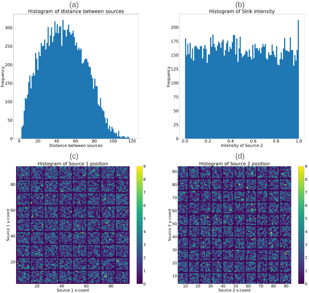
The data used in this paper is motivated by biological multiscale modeling [15], and correspond to two sources placed in a lattice with a decay rate which acts as a sink. To generate representative initial conditions and corresponding steady-state diffusion fields from a two-source system, we consider a 100x100 lattice. In total, 20k initial configurations were created with two sources randomly positioned in the lattice. Each source, characterized by a 5-unit radius, has a constant flux of 1 for one source, while the other sources have a randomly assigned constant flux value between 0 and 1, randomly assigned using a uniform distribution. The remainder of the lattice has a field value of zero. The stationary solution to the diffusion equation with absorbing boundary conditions for each initial condition is computed using the Differential Equation package in Julia [21]. We denote as the input image that represents the initial condition layout of the two source cells, and represents the output image, which is the predicted stationary solution of the diffusion equation.
The diffusion constant is set to and the decay rate , resulting in a diffusion length . This length diminishes as increases and as decreases. A decrease in this length corresponds to a reduction in the field gradient as explained in [54]. Figure 1 summarizes the distribution of some of the key parameters, including the distance between the two sources (a), the intensity of one source (b), and the positions of the two sources (c-d). The code for the generation of data and the data can be found [55, 15].
3.2 DNN Surrogates
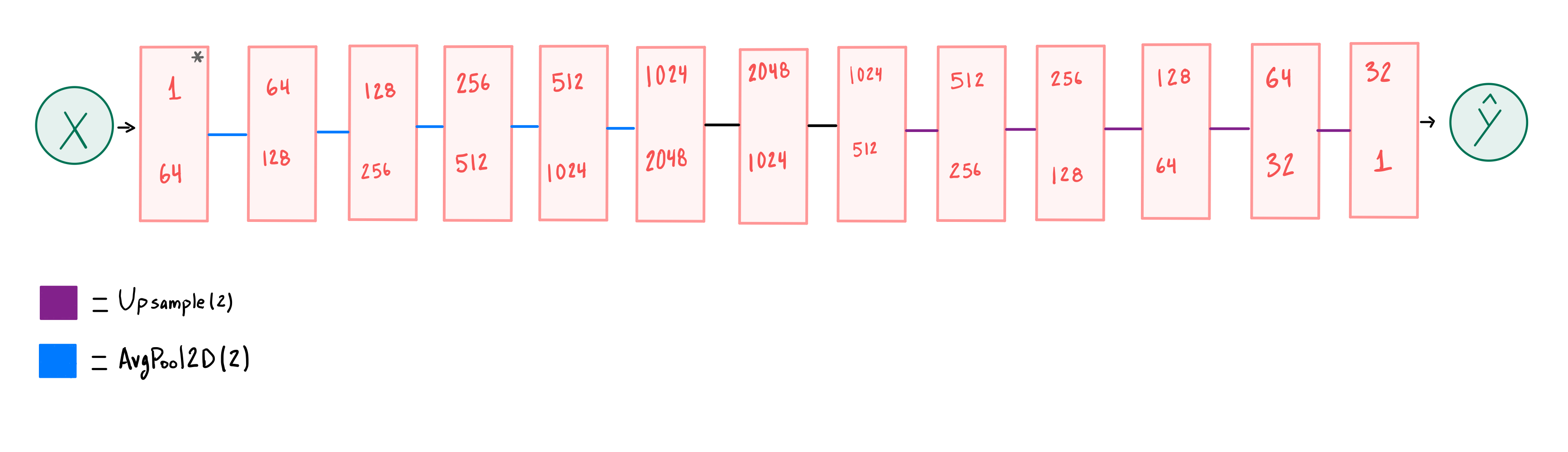
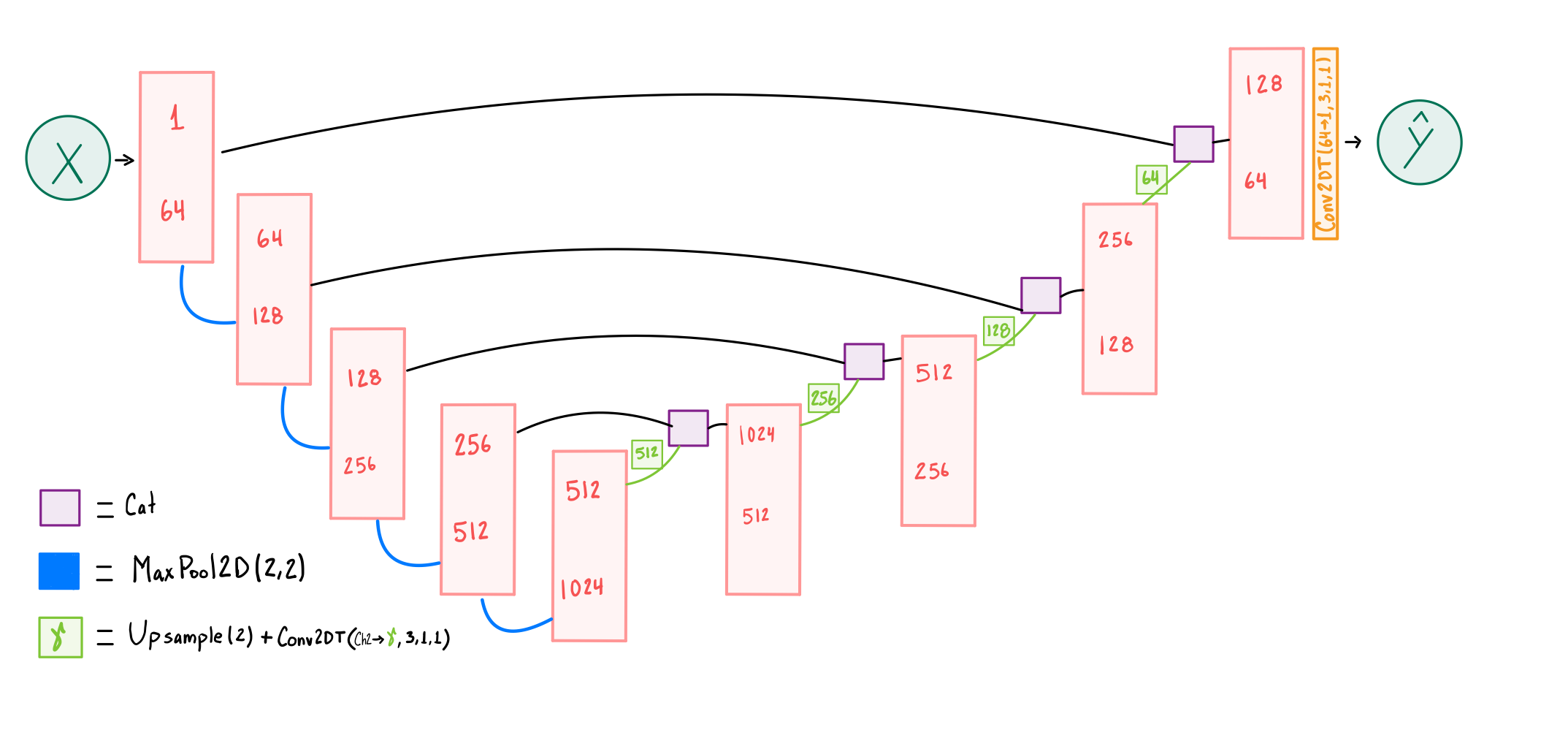
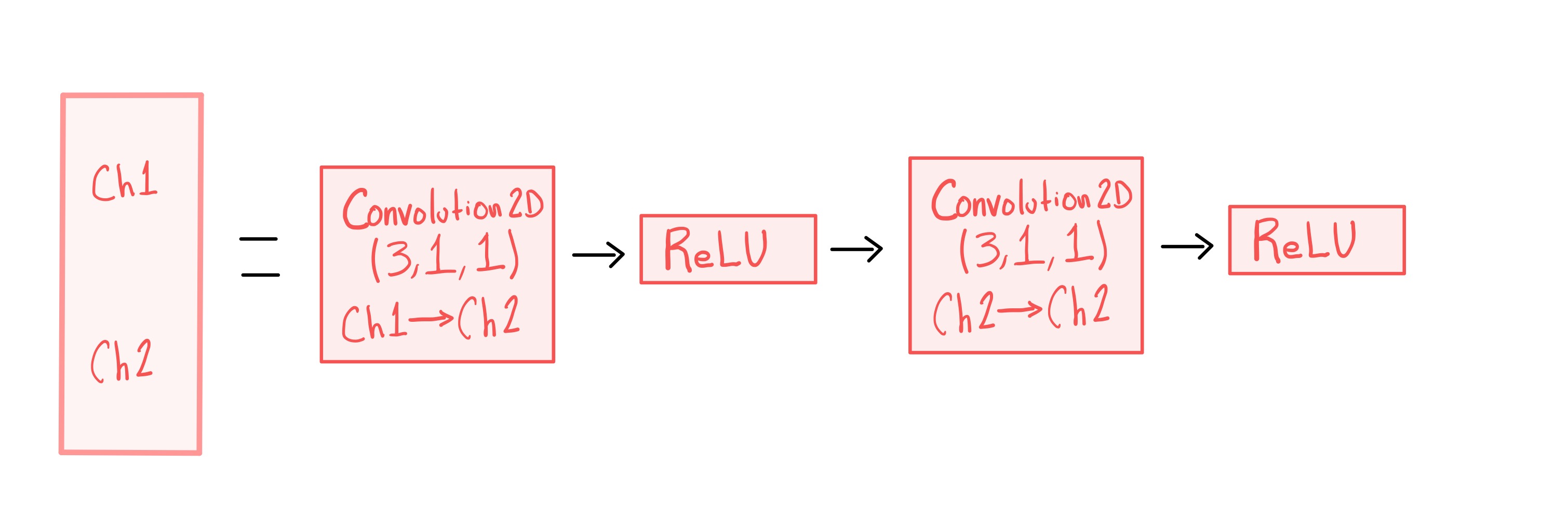
We define two DNN architectures, namely, a CNN based autoencoder and an U-Net-based structure as shown in Figure 3 and 3, respectively.
The autoencoder’s first six layers perform an average-pool operation that reduces height and width in half after each layer following the sequence {, , , , , , } while adding channels after each layer following the sequence {1, 64, 128, 256, 512, 1024, 2048}. Similar to [15], the next six layers reduce the number of channels while increasing the height and width in the opposite order from those described above.
The first four layers of the U-Net perform max-pool operation, which, similar to CNN autoencoder, reduces the height and width to half following the sequence {, , , and } with corresponding channels of {1, 64, 128, 256 and 512 } until the bottleneck is reached, where the size is with channels. The subsequent four layers reverse this process, upscaling the image starting from the bottleneck and concatenating images from the downscaling side to produce features with sizes and channels opposite to those described earlier. A final layer adjusts the number of channels from to and the image size to .
3.3 Loss Definition
One of the sources in the input images has an intensity of 1, while the other has a uniformly distributed random number. The two sources occupy 2% of the total image space, with the rest of the space with intensity 0. Due to the disproportionate distribution of source and space intensity, the source pixels need to be weighed to avoid high field values to wash out. The loss is thus weighed with an exponential weight and modulated with a scalar hyperparameter .
| (1) |
where is set to 1 and represents the input and target tuple. We refer to this as weighted mean absolute error (MAE) in the remainder of this paper. Here denotes the inner product and is a unitary vector with the same size as with all components equal to zero except the element in position which is equal to one. is a vector with all components equal to 1 and size equal to . Then is a scalar corresponding to the pixel value at the position in , whereas for all . Notice that high and low pixel values will have an exponential weight and , respectively. This implies that the error associated with high pixels will have a larger value than that for low pixels. The loss function is the mean value over all pixels and a given data set
4 Methods: Active Learning of DNN Surrogates for Diffusion Solvers
4.1 Active Learning
Let be the complete input and output training data pair divided into the initially labeled set and the remaining unlabeled data . We initially train the diffusion surrogate model with the and evaluate the acquisition function on . most informative data from are labeled and appended to such that and . The model is retrained on the labeled data and the process iterates until a performance metric is reached or a total labeled data size reaches .
Note that an important consideration for the design of acquisition functions is that the labels (in this case the simulation outputs on the given inputs) of the samples are not available before the samples are selected to be queried for label. In another word, the acquisition objective cannot utilize the label of the samples. We consider three active learning acquisition functions and compare them with random acquisition. Two are representative of uncertainty-based acquisitions, including the use of entropy [32] and the estimated loss of the DNN surrogage [31]. One is representative of acquisitions considering the diversity of training samples.
Entropy:
Entropy sampling [32] selects instances that the model is most uncertain about as measured by the standard deviation of the ’k’ output predictions of the network. We use dropout as Bayesian approximation [33] to generate ’k’ different output predictions and evaluate entropy as:
| (2) |
where, is the pixel in the prediction, is the mean prediction of the pixel obtained through ’k’ forward passes with dropout and are the total number of pixels in the lattice.
Temporal Output Discrepancy (TOD):
The loss of the DNN surrogate on a new sample is another potential criteria for selecting samples a DNN is most uncertain about: a high-loss sample has the potential to provide stronger signals for the optimization of the DNN, whereas a low-loss sample could be redundant to what the DNN is already trained with. Intended as a criteria for selecting unlabeled data samples, the loss of the DNN on the unlabeled samples cannot be calculated from the actual labels (here the simulation outputs) but must be estimated. Following the Temporal Output Discrepancy (TOD) measure [31], we estimate the DNN loss on a sample based on the discrepancy of the DNN outputs on the same sample at different learning iterations:
| (3) |
where is the distance between outputs of the model with parameter and evaluated at and gradient optimization step. In our experiments, we set .
To ground the results obtained from TOD, we also use the actual loss of a new sample as the acquisition criteria owing to the existence of simulation data already generated offline. Once we train the DNN surrogate on the labeled data , we calculate the loss of the unlabelled data with the available simulation outputs and select examples with the highest losses to add to for the next training. Note that this is intended to provide a reference for the efficacy of TOD that is reliant on an estimation of the DNN loss on unlabled samples, not an acquisition strategy to be used during active learning of DNN surrogates (as true loss is not available on unlabeled new samples).
Parameter Diversity:
To consider the diversity of training simulations without looking at the simulated outputs, we measure diversity by the parameters used to generate the simulations. We consider six parameters in the input initial condition, including the coordinates (cx and cy) of the two sources (), the distance between the sources (), and the intensity of the second source () as the important identifiers () for the model. Following [39], we create a coreset subset from the unlabeled data such that the examples with the largest minimal distance from the labeled data are selected.
| (4) |
We select examples from that have maximum calculated parameter diversity distance .
4.2 Evaluation Metrics
Weighted-MAE
We assess the DNN surrogate’s performance by calculating its loss, i.e., its weighted mean absolute error, as defined in Equation 1. After each acquisition round, the metric is computed on the test data for all active learning acquisition functions.
Region-of-Interest MAE
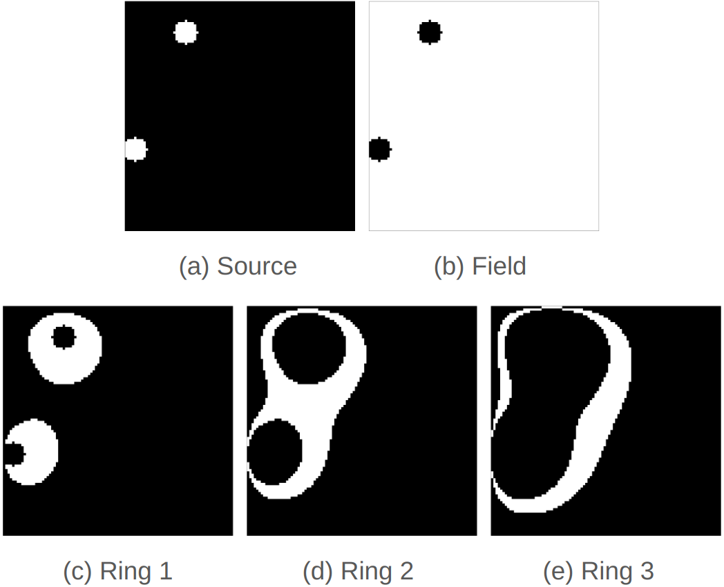
As mentioned earlier, the sources occupy 2% of the total lattice space where the diffusion pattern emanate from the source and die out quickly in the field. To better understand the effect of active learning on the accuracy of DNN surrogates, we further examine the MAE in different regions of interest on the lattice as illustrated in Figure 4: the regions of "Source" and "Field" are determined based on the initial inputs to the simulations; the regions of "RINGS 1," "RINGS 2," and "RINGS 3" are defined based on the ground-truth simulation outputs using pixel values in the ranges [0.2, 1.0], [0.1, 0.2], and [0.05, 0.1], respectively – representing increasing distances to the sources.
5 Experiments
We split the two-source data described in section 3.1. into 16,000 training data, 4,000 validation data, and 4,000 test data. We trained the U-Net and CNN autoencoder structure defined in section 3.2. We divided the 16000 training data into an initial 1000 labelled data (samples with simulation outputs available) and a 15000 unlabelled pool (samples without simulation outputs). We performed active learning with the acquisition functions defined in section 4.1 for CNN autoencoder and exclude entropy acquisition function for U-Net due to large computational demand for forward passes. At each acquisition round, new unlabled samples are selected to query for simulation outputs, and the DNN surrogates were retrained with the current labeled dataset (input-output simulationp pairs). This was repeated until all the 15000 unlabelled samples are labeled. In each active learning round, the DNN surrogate was trained for 500 epochs and saved based on the best validation loss. For the entropy acquisition function, in CNN autoencoder, 40% dropouts were added after batch normalization of the first and second convolutional layers. The code repository can be found in [56].
5.1 Comparison of Active Learning Acquisition Functions
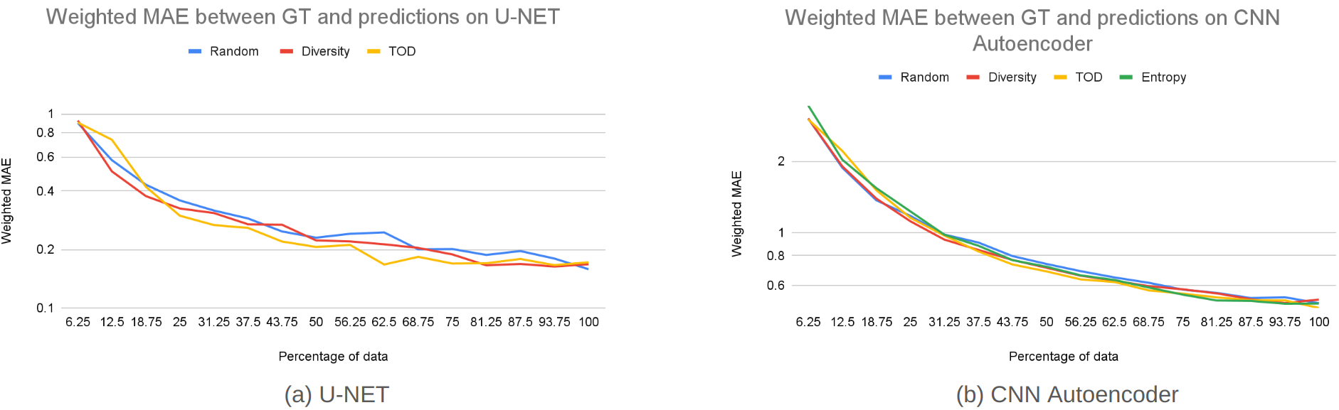
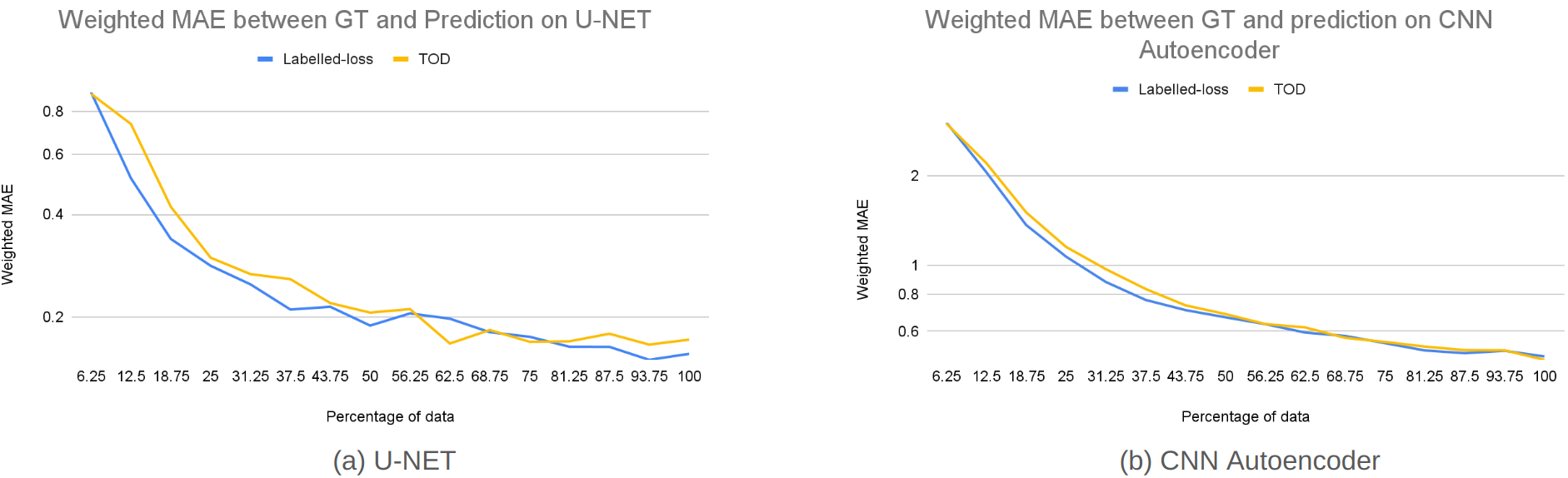
Figure 6(a) compares weighted-MAE between the ground truth and DNN surrogate predictions for different acquisition functions at different percentages of labeled data, evaluated against random acquisitions for the U-Net architecture. As shown, actively selecting simulation data for DNN surrogates training, especially by considering the estimated loss of the surrogate (TOD), consistently improves the DNN performance compared to random acquisition using the same amount of labeled training data. Note that TOD, even though reliant on an estimate of the DNN loss without the simulation output as labels, acquires a performance on par with using the actual DNN loss calculated from labels as shown in Figure 6(a). In comparison, diversity-based selection of training samples demonstrated limited benefits with a performance similar to or marginally better than random acquisition.
Table 1 lists the weighted MAE between the simulated ground truth and predictions on the test data for U-Net across quarterly percentages of labeled data, computed for the different regions of interest as described in Figure 4. The results show that, at the same amount of labeled training data throughout the active learning process, the careful selection of training simulations achieved a test performance improvement across all acquisition strategies (except when all data are used): this improvement was more evident when the size of the labeled data was small. Additionally, these improvements were more pronounced at the regions proximal to the source (SRC, RING1) where the errors were the highest. This observation can be better appreciated in visual examples of the absolute errors (Figure 7) between DNN surrogate predictions and ground-truth simulation outputs obtained on the U-Net architecture. As expected, across the three rows, there is a gradual decrease in error as the training data increases. Notably, however, TOD consistently exhibits lower errors compared to random training, especially in regions close to the sources.
| Test Loss for U-Net | Test Loss for CNN Autoencoder | |||||||||||
|---|---|---|---|---|---|---|---|---|---|---|---|---|
| DATA SIZES | DATA SIZES | |||||||||||
| 25% | 50% | 75% | 100% | 25% | 50% | 75% | 100% | |||||
| Random | 0.35784 | 0.23011 | 0.20112 | 0.15839 | Random | 1.17626 | 0.73720 | 0.57466 | 0.50335 | |||
| Diverse | 0.32529 | 0.22275 | 0.18868 | 0.16786 | Diverse | 1.11622 | 0.71032 | 0.57625 | 0.52171 | |||
| TOD | 0.29847 | 0.20616 | 0.16936 | 0.16616 | ALL | TOD | 1.15445 | 0.68581 | 0.55251 | 0.48098 | ||
| Entropy | 1.22860 | 0.71770 | 0.54734 | 0.50217 | ALL | |||||||
| Random | 4.92366 | 3.13306 | 2.75548 | 2.19644 | Random | 18.46547 | 11.72694 | 8.68628 | 7.60275 | |||
| Diverse | 4.41641 | 2.96436 | 2.52532 | 2.17466 | Diverse | 18.03126 | 11.03576 | 8.59056 | 7.99048 | |||
| TOD | 3.58799 | 2.91486 | 2.07431 | 2.33184 | SRC | TOD | 18.29991 | 10.79857 | 8.45668 | 7.16640 | ||
| Entropy | 18.48527 | 11.08221 | 8.19734 | 7.73362 | SRC | |||||||
| Random | 1.48035 | 0.94344 | 0.84136 | 0.63358 | Random | 5.33343 | 3.30900 | 2.63469 | 2.31095 | |||
| Diverse | 1.41882 | 0.92979 | 0.79940 | 0.69533 | Diverse | 5.01338 | 3.22305 | 2.65821 | 2.36826 | |||
| TOD | 1.15558 | 0.82894 | 0.69378 | 0.67992 | RING1 | TOD | 5.02481 | 3.06267 | 2.51028 | 2.19476 | ||
| Entropy | 5.52691 | 3.20892 | 2.48799 | 2.27788 | RING1 | |||||||
| Random | 0.34664 | 0.23742 | 0.19985 | 0.17337 | Random | 0.90847 | 0.57265 | 0.45602 | 0.39152 | |||
| Diverse | 0.30417 | 0.23389 | 0.18549 | 0.17087 | Diverse | 0.86313 | 0.54783 | 0.44496 | 0.41255 | |||
| TOD | 0.37816 | 0.21057 | 0.19488 | 0.17043 | RING2 | TOD | 1.00724 | 0.54755 | 0.43630 | 0.38701 | ||
| Entropy | 1.03330 | 0.59488 | 0.44425 | 0.39372 | RING2 | |||||||
| Random | 0.14096 | 0.09395 | 0.07416 | 0.06339 | Random | 0.27176 | 0.17411 | 0.13709 | 0.11720 | |||
| Diverse | 0.11276 | 0.08636 | 0.06804 | 0.07206 | Diverse | 0.25081 | 0.16577 | 0.13732 | 0.12434 | |||
| TOD | 0.15077 | 0.08337 | 0.07653 | 0.06613 | RING3 | TOD | 0.30949 | 0.17163 | 0.13658 | 0.11916 | ||
| Entropy | 0.31644 | 0.18589 | 0.13581 | 0.12081 | RING3 | |||||||
| Random | 0.28301 | 0.18254 | 0.15927 | 0.12500 | Random | 0.89296 | 0.55713 | 0.44174 | 0.38700 | |||
| Diverse | 0.25827 | 0.17783 | 0.15039 | 0.13497 | Diverse | 0.83903 | 0.54113 | 0.44492 | 0.39932 | |||
| TOD | 0.24457 | 0.16177 | 0.13815 | 0.13069 | FIELD | TOD | 0.87351 | 0.52009 | 0.42297 | 0.37143 | ||
| Entropy | 0.94582 | 0.54786 | 0.42197 | 0.38366 | FIELD | |||||||
Overall, TOD was able to use a smaller amount of data (50%) to achieve the performance random acquisition can achieve with a higher amount of data (75%). Note that we do not expect significant differences between different acquisition strategies when 100% data are used.
5.2 Effect of Architecture on Active Learning
Figure 8 first compares the results obtained by U-Net and CNN autoencoder when 100% data were used, which shows that CNN autoencoder was suboptimal as a surrogate architecture compared to the U-Net for the diffusion equations.
Figure 6(b) compares the weighted MAE for the CNN autoencoder at different percentages of labeled data across different acquisition functions. Compared with Figure 6(a), it is apparent that despite using identical acquisition functions and datasets, the performance improvements due to active learning is more pronounced in U-Net architecture compared to CNN autoencoder: the performance gain due to active learning for the CNN autoencoder is marginal at best with random training. This distinction is also evident in the quantitative data presented in Table 1. Similarly, as shown in the the visual examples of the absolute error maps between ground-truth simulations and surrogate predictions presented in Figure 9, in contrast to our previous observations on the U-Net, the errors among the acquisition functions remain consistently similar.
These results suggest an interesting and important finding: for active selection of training simulations to play a role in the construction of DNN surrogates, it is important to first identify an appropriate if not optimal DNN architecture for the surrogate, as the choices of architectures have a significant effect on the relative ranking of various acquisition function and the benefit they can deliver. Interestingly, this result is consistent with those reported systematic evaluations of general DAL methods [57, 58].
6 Discussion
In this paper, we investigate the feasibility of integrating active learning in the training of a DNN surrogate for the diffusion solver. Our findings highlight two key observations. Firstly, training a DNN surrogate with intelligently selected simulations has the potential to reduce the requirement on the generation of expensive simulations and improve the performance of the DNN surrogates. Specifically, acquisition strategies focused on the predicted loss of the DNN surrogates on new samples may be the most promising for training smart DNN surrogates. This encourages the use of active learning in training surrogate models with less but informative data rather than a pre-annotated dataset. Secondly, the choice of network itself significantly impacts the benefit derived from active learning: with the same data and acquisition strategies, to what extent the active learning improves the DNN surrogate training largely depends on the underlying choice of DNN architecture – CNN autoencoder versus U-Net in this case. This suggests that, to develop a HPC infrastructure that support the construction of Smart Surrogate with active learning, an additional component that needs to be supported by the infrastructure may be the optimization of the DNN surrogate architecture prior to active learning.
As a first proof-of-concept feasibility study, future works can be improved along the following fronts.
Diversification of Applications and Dataset Scales
While our current work is focused on a use case of diffusion solver surrogate with two sources randomly placed on a lattice, we plan on incorporating a larger simulation set. This set will feature a variable number of sources on a larger lattice, capturing inherent randomness in real world simulations. Furthermore, we recognize the importance to broaden our application scope, transcending the confines of our current focus to encompass a diverse array of use cases.
Broader Spectrums of Acquisition Functions
Our study currently incorporates three distinctive acquisition functions, serving as the foundation for exploring the integration of active learning into surrogate training. Owing to the ever-developing field of active learning field, our future plans involve the inclusion of additional acquisition functions that leverage evidential uncertainty and hybrid strategies, combining the benefit of uncertainty and diversity.
Expansive Exploration of Architectural Impact
The interplay between active learning performance and architecture as observed in this study provides important insight into the importance of optimal architectural design and training data selection in building DNN surrogates. Future works will entail an empirical study over a larger architecture space and even branching out to fields like architecture optimization and network architecture search.
Transition to Smart Surrogates: On-the-Fly Simulations Steered by Active Learning
This study, although based on simulation data generated offline, provide important insights into the feasibility and key design elements for active learning of DNN surrogates. As a pivotal shift in our research trajectory, we are moving from offline emulation to online scenarios where HPC simulations will be steered and executed on the fly by active learning. While the methodological framework presented in this study will generally apply with minimal modifications, substantial efforts will be needed to establish the HPC infrastructure that can support on-the-fly allocation of different HPC resources in between the execution of high-performance simulations, DNN training, and decision-making of data acquisitions – an exciting next step of the current study.
7 Conclusion
We present an investigative study that underscores the benefit of utilizing active learning in training a diffusion solver surrogate model. We experimentally show that for certain acquisition functions, active learning with fewer data (<50% data) shows promise in improving over training randomly with larger data size (>75% data). This provides a strong foundation for the next steps to build up the HPC infrastructure of Smart Surrogates where training simulations are generated on the fly as steered by active learning, potentially on a DNN architecture optimized for the scientific simulations at hand.
8 Acknowledgements
This work is supported by National Science Foundation funding NSF OAC-2212548 and NSF OAC-2212550.
References
- [1] Geoffrey Fox and Shantenu Jha. Learning everywhere: a taxonomy for the integration of machine learning and simulations. In 2019 15th International Conference on eScience (eScience), pages 439–448. IEEE, 2019.
- [2] Shantenu Jha and Geoffrey Fox. Understanding ml driven hpc: applications and infrastructure. In 2019 15th International Conference on eScience (eScience), pages 421–427. IEEE, 2019.
- [3] Geoffrey Fox, James A Glazier, JCS Kadupitiya, Vikram Jadhao, Minje Kim, Judy Qiu, James P Sluka, Endre Somogyi, Madhav Marathe, Abhijin Adiga, et al. Learning everywhere: Pervasive machine learning for effective high-performance computation. In 2019 IEEE International Parallel and Distributed Processing Symposium Workshops (IPDPSW), pages 422–429. IEEE, 2019.
- [4] Muhammad Firmansyah Kasim, D Watson-Parris, L Deaconu, S Oliver, P Hatfield, Dustin H Froula, Gianluca Gregori, M Jarvis, S Khatiwala, J Korenaga, et al. Building high accuracy emulators for scientific simulations with deep neural architecture search. Machine Learning: Science and Technology, 3(1):015013, 2021.
- [5] Eugen Hruska, Vivekanandan Balasubramanian, Hyungro Lee, Shantenu Jha, and Cecilia Clementi. Extensible and scalable adaptive sampling on supercomputers. Journal of Chemical Theory and Computation, 16(12):7915–7925, 2020.
- [6] Hyungro Lee, Matteo Turilli, Shantenu Jha, Debsindhu Bhowmik, Heng Ma, and Arvind Ramanathan. Deepdrivemd: Deep-learning driven adaptive molecular simulations for protein folding. In 2019 IEEE/ACM Third Workshop on Deep Learning on Supercomputers (DLS), pages 12–19. IEEE, 2019.
- [7] Andreas Mardt, Luca Pasquali, Hao Wu, and Frank Noé. Vampnets for deep learning of molecular kinetics. Nature communications, 9(1):5, 2018.
- [8] Debsindhu Bhowmik, Shang Gao, Michael T Young, and Arvind Ramanathan. Deep clustering of protein folding simulations. BMC bioinformatics, 19:47–58, 2018.
- [9] Anh-Tien Ton, Francesco Gentile, Michael Hsing, Fuqiang Ban, and Artem Cherkasov. Rapid identification of potential inhibitors of sars-cov-2 main protease by deep docking of 1.3 billion compounds. Molecular informatics, 39(8):2000028, 2020.
- [10] Zhirui Liao, Ronghui You, Xiaodi Huang, Xiaojun Yao, Tao Huang, and Shanfeng Zhu. Deepdock: enhancing ligand-protein interaction prediction by a combination of ligand and structure information. In 2019 IEEE International Conference on Bioinformatics and Biomedicine (BIBM), pages 311–317. IEEE, 2019.
- [11] Austin Clyde, Xiaotian Duan, and Rick Stevens. Regression enrichment surfaces: a simple analysis technique for virtual drug screening models. arXiv preprint arXiv:2006.01171, 2020.
- [12] Luning Sun, Han Gao, Shaowu Pan, and Jian-Xun Wang. Surrogate modeling for fluid flows based on physics-constrained deep learning without simulation data. Computer Methods in Applied Mechanics and Engineering, 361:112732, 2020.
- [13] Han Gao, Luning Sun, and Jian-Xun Wang. Phygeonet: Physics-informed geometry-adaptive convolutional neural networks for solving parameterized steady-state pdes on irregular domain. Journal of Computational Physics, 428:110079, 2021.
- [14] Mustafa Mustafa, Deborah Bard, Wahid Bhimji, Zarija Lukić, Rami Al-Rfou, and Jan M Kratochvil. Cosmogan: creating high-fidelity weak lensing convergence maps using generative adversarial networks. Computational Astrophysics and Cosmology, 6(1):1–13, 2019.
- [15] J Quetzalcóatl Toledo-Marín, Geoffrey Fox, James P Sluka, and James A Glazier. Deep learning approaches to surrogates for solving the diffusion equation for mechanistic real-world simulations. Frontiers in Physiology, 12:667828, 2021.
- [16] Winfried van den Dool, Tijmen Blankevoort, Max Welling, and Yuki Asano. Efficient neural pde-solvers using quantization aware training. In Proceedings of the IEEE/CVF International Conference on Computer Vision, pages 1423–1432, 2023.
- [17] Olaf Ronneberger, Philipp Fischer, and Thomas Brox. U-net: Convolutional networks for biomedical image segmentation. In Medical Image Computing and Computer-Assisted Intervention–MICCAI 2015: 18th International Conference, Munich, Germany, October 5-9, 2015, Proceedings, Part III 18, pages 234–241. Springer, 2015.
- [18] Jayesh K Gupta and Johannes Brandstetter. Towards multi-spatiotemporal-scale generalized pde modeling. arXiv preprint arXiv:2209.15616, 2022.
- [19] Jacob Fish Ted Belytschko. A first course in finite elements. 2007.
- [20] William E Schiesser. The numerical method of lines: integration of partial differential equations. Elsevier, 2012.
- [21] Christopher Rackauckas and Qing Nie. Differentialequations. jl–a performant and feature-rich ecosystem for solving differential equations in julia. Journal of open research software, 5(1), 2017.
- [22] Amir Barati Farimani, Joseph Gomes, and Vijay S Pande. Deep learning the physics of transport phenomena. arXiv preprint arXiv:1709.02432, 2017.
- [23] Jiequn Han, Arnulf Jentzen, and Weinan E. Solving high-dimensional partial differential equations using deep learning. Proceedings of the National Academy of Sciences, 115(34):8505–8510, 2018.
- [24] Zongyi Li, Nikola Kovachki, Kamyar Azizzadenesheli, Burigede Liu, Kaushik Bhattacharya, Andrew Stuart, and Anima Anandkumar. Fourier neural operator for parametric partial differential equations. arXiv preprint arXiv:2010.08895, 2020.
- [25] Haiyang He and Jay Pathak. An unsupervised learning approach to solving heat equations on chip based on auto encoder and image gradient. arXiv preprint arXiv:2007.09684, 2020.
- [26] Jared Willard, Xiaowei Jia, Shaoming Xu, Michael Steinbach, and Vipin Kumar. Integrating physics-based modeling with machine learning: A survey. arXiv preprint arXiv:2003.04919, 1(1):1–34, 2020.
- [27] Shengze Cai, Zhicheng Wang, Sifan Wang, Paris Perdikaris, and George Em Karniadakis. Physics-informed neural networks for heat transfer problems. Journal of Heat Transfer, 143(6):060801, 2021.
- [28] J Quetzalcoatl Toledo-Marin, James A Glazier, and Geoffrey Fox. Analyzing the performance of deep encoder-decoder networks as surrogates for a diffusion equation. arXiv preprint arXiv:2302.03786, 2023.
- [29] David A Cohn, Zoubin Ghahramani, and Michael I Jordan. Active learning with statistical models. Journal of artificial intelligence research, 4:129–145, 1996.
- [30] Donggeun Yoo and In So Kweon. Learning loss for active learning. In Proceedings of the IEEE/CVF conference on computer vision and pattern recognition, pages 93–102, 2019.
- [31] Siyu Huang, Tianyang Wang, Haoyi Xiong, Jun Huan, and Dejing Dou. Semi-supervised active learning with temporal output discrepancy. In Proceedings of the IEEE/CVF International Conference on Computer Vision, pages 3447–3456, 2021.
- [32] Ajay J Joshi, Fatih Porikli, and Nikolaos Papanikolopoulos. Multi-class active learning for image classification. In 2009 IEEE Conference on Computer Vision and Pattern Recognition, pages 2372–2379. IEEE, 2009.
- [33] Yarin Gal and Zoubin Ghahramani. Dropout as a bayesian approximation: Representing model uncertainty in deep learning. In international conference on machine learning, pages 1050–1059. PMLR, 2016.
- [34] Neil Houlsby, Ferenc Huszár, Zoubin Ghahramani, and Máté Lengyel. Bayesian active learning for classification and preference learning. arXiv preprint arXiv:1112.5745, 2011.
- [35] Andreas Kirsch, Joost Van Amersfoort, and Yarin Gal. Batchbald: Efficient and diverse batch acquisition for deep bayesian active learning. Advances in neural information processing systems, 32, 2019.
- [36] Dan Roth and Kevin Small. Margin-based active learning for structured output spaces. In Machine Learning: ECML 2006: 17th European Conference on Machine Learning Berlin, Germany, September 18-22, 2006 Proceedings 17, pages 413–424. Springer, 2006.
- [37] Tobias Scheffer, Christian Decomain, and Stefan Wrobel. Active hidden markov models for information extraction. In International Symposium on Intelligent Data Analysis, pages 309–318. Springer, 2001.
- [38] Burr Settles. Active learning literature survey. 2009.
- [39] Ozan Sener and Silvio Savarese. Active learning for convolutional neural networks: A core-set approach. arXiv preprint arXiv:1708.00489, 2017.
- [40] Yonatan Geifman and Ran El-Yaniv. Deep active learning over the long tail. arXiv preprint arXiv:1711.00941, 2017.
- [41] Hieu T Nguyen and Arnold Smeulders. Active learning using pre-clustering. In Proceedings of the twenty-first international conference on Machine learning, page 79, 2004.
- [42] Min Wang, Fan Min, Zhi-Heng Zhang, and Yan-Xue Wu. Active learning through density clustering. Expert systems with applications, 85:305–317, 2017.
- [43] Keze Wang, Dongyu Zhang, Ya Li, Ruimao Zhang, and Liang Lin. Cost-effective active learning for deep image classification. IEEE Transactions on Circuits and Systems for Video Technology, 27(12):2591–2600, 2016.
- [44] Zongwei Zhou, Jae Shin, Lei Zhang, Suryakanth Gurudu, Michael Gotway, and Jianming Liang. Fine-tuning convolutional neural networks for biomedical image analysis: actively and incrementally. In Proceedings of the IEEE conference on computer vision and pattern recognition, pages 7340–7351, 2017.
- [45] Lin Yang, Yizhe Zhang, Jianxu Chen, Siyuan Zhang, and Danny Z Chen. Suggestive annotation: A deep active learning framework for biomedical image segmentation. In Medical Image Computing and Computer Assisted Intervention- MICCAI 2017: 20th International Conference, Quebec City, QC, Canada, September 11-13, 2017, Proceedings, Part III 20, pages 399–407. Springer, 2017.
- [46] Jordan T Ash, Chicheng Zhang, Akshay Krishnamurthy, John Langford, and Alekh Agarwal. Deep batch active learning by diverse, uncertain gradient lower bounds. arXiv preprint arXiv:1906.03671, 2019.
- [47] Changjian Shui, Fan Zhou, Christian Gagné, and Boyu Wang. Deep active learning: Unified and principled method for query and training. In International Conference on Artificial Intelligence and Statistics, pages 1308–1318. PMLR, 2020.
- [48] Haonan Wang, Wei Huang, Ziwei Wu, Hanghang Tong, Andrew J Margenot, and Jingrui He. Deep active learning by leveraging training dynamics. Advances in Neural Information Processing Systems, 35:25171–25184, 2022.
- [49] Seo Taek Kong, Soomin Jeon, Dongbin Na, Jaewon Lee, Hong-Seok Lee, and Kyu-Hwan Jung. A neural pre-conditioning active learning algorithm to reduce label complexity. Advances in Neural Information Processing Systems, 35:32842–32853, 2022.
- [50] Dongxia Wu, Ruijia Niu, Matteo Chinazzi, Alessandro Vespignani, Yi-An Ma, and Rose Yu. Deep bayesian active learning for accelerating stochastic simulation. In Proceedings of the 29th ACM SIGKDD Conference on Knowledge Discovery and Data Mining, pages 2559–2569, 2023.
- [51] Raphaël Pestourie, Youssef Mroueh, Thanh V Nguyen, Payel Das, and Steven G Johnson. Active learning of deep surrogates for pdes: application to metasurface design. npj Computational Materials, 6(1):164, 2020.
- [52] Kjetil O Lye, Siddhartha Mishra, Deep Ray, and Praveen Chandrashekar. Iterative surrogate model optimization (ismo): An active learning algorithm for pde constrained optimization with deep neural networks. Computer Methods in Applied Mechanics and Engineering, 374:113575, 2021.
- [53] L Zanisi, A Ho, T Madula, J Barr, J Citrin, S Pamela, J Buchanan, F Casson, V Gopakumar, et al. Efficient training sets for surrogate models of tokamak turbulence with active deep ensembles. arXiv preprint arXiv:2310.09024, 2023.
- [54] Andreĭ Nikolaevich Tikhonov and Aleksandr Andreevich Samarskii. Equations of mathematical physics. Courier Corporation, 2013.
- [55] J. Quetzalcoatl Toledo-Marin. Steady state diffusion equation. https://github.com/jquetzalcoatl/DiffSolver, 2023.
- [56] Pradeep Bajracharya. Active learning with diffusion surrogate. https://github.com/pb8294/active-diffusion, 2023.
- [57] Nathan Beck, Durga Sivasubramanian, Apurva Dani, Ganesh Ramakrishnan, and Rishabh Iyer. Effective evaluation of deep active learning on image classification tasks. arXiv preprint arXiv:2106.15324, 2021.
- [58] Prateek Munjal, Nasir Hayat, Munawar Hayat, Jamshid Sourati, and Shadab Khan. Towards robust and reproducible active learning using neural networks. In Proceedings of the IEEE/CVF Conference on Computer Vision and Pattern Recognition, pages 223–232, 2022.