Satellite image classification with neural quantum kernels

Abstract

A practical application of quantum machine learning in real-world scenarios in the short term remains elusive, despite significant theoretical efforts. Image classification, a common task for classical models, has been used to benchmark quantum algorithms with simple datasets, but only few studies have tackled complex real-data classification challenges. In this work, we address such a gap by focusing on the classification of satellite images, a task of particular interest to the earth observation (EO) industry. We first preprocess the selected intrincate dataset by reducing its dimensionality. Subsequently, we employ neural quantum kernels (NQKs) -embedding quantum kernels (EQKs) constructed from trained quantum neural networks (QNNs)- to classify images which include solar panels. We explore both $1$-to-$n$ and $n$-to-$n$ NQKs. In the former, parameters from a single-qubit QNN’s training construct an $n$-qubit EQK achieving a mean test accuracy over 86% with three features. In the latter, we iteratively train an $n$-qubit QNN to ensure scalability, using the resultant architecture to directly form an $n$-qubit EQK. In this case, a test accuracy over 88% is obtained for three features and 8 qubits. Additionally, we show that the results are robust against a suboptimal training of the QNN.

I Introduction

Recent advancements in the field of quantum machine learning (QML) Biamonte et al. (2017); Carleo et al. (2019); Dunjko and Briegel (2018) have significantly enhanced our understanding of how quantum resources can be utilized to design various new paradigms Huang et al. (2021a); Schuld (2021); Jerbi et al. (2023); Schuld and Killoran (2019). These developments have shed light on the trainability McClean et al. (2018); Cerezo et al. (2021); Holmes et al. (2022); Fontana et al. (2024); Ragone et al. (2023); Thanasilp et al. (2024); Pesah et al. (2021) and generalization capabilities of quantum models Caro et al. (2021, 2022); Peters and Schuld (2023); Banchi et al. (2021); Gil-Fuster et al. (2024) and have even demonstrated theoretical advantages over classical methods for certain tailored problems Gyurik and Dunjko (2023); Sweke et al. (2021); Jerbi et al. (2021); Liu et al. (2021); Pirnay et al. (2023). Despite these breakthroughs and the successful implementation of quantum models on quantum processors Havlíček et al. (2019); Johri et al. (2021); Ristè et al. (2017); Steinbrecher et al. (2019); Peters et al. (2021), the practicality of QML remains uncertain Jadhav et al. (2023).

Image classification is one of the most usfeul tasks due to its significant industrial applications. Various approaches have been explored, including quantum convolutional neural networks (QCNNs)Matic et al. (2022); Henderson et al. (2020a); Lü et al. (2021); Chen et al. (2023) and models that leverage symmetries Chang et al. (2023); West et al. (2023); Sebastian et al. (2024); West et al. (2024). There is increasing recognition that combining classical and quantum approaches can be more beneficial than trying to replace one by the other. The pursuit of better machine learning techniques with new methodologies involves a deeper consideration of various factors such as resource efficiency, data requirements, and the practical applications of these technologies. As addressed in this work, this involves pre-processing images classically before applying a quantum data processing model Senokosov et al. (2024); Dang et al. (2018). The aim is to demonstrate the development and implementation of models using components executable on quantum processors, with the goal of scaling them up to create models that cannot be simulated on classical processors.

Most studies in this context focus on typical classification problems that serve as benchmarks for evaluating these models, while just a few address more realistic classification challenges. Earth observation (EO), with the use of remote sensing technologies, provides valuable data for a wide range of applications, including climate change monitoring, disaster management, agricultural productivity assessment, and urban planning. By using machine learning, EO has become essential for extracting useful insights from this data, helping us manage Earth’s systems more effectively. Recently, the daily volume of satellite image products has surged significantly due to a wide range of institutional and commercial missions () (ESA); Commission (2018). This growth has prompted the EO community to explore computational paradigms that could enhance current methods.

Not many studies have tackled this complex classification task using quantum resources. The prevalent approach involves using parameterized quantum circuits following dimensionality reduction techniques, as seen in Refs. Zollner et al. (2024); Sebastianelli et al. (2022); Benítez-Buenache and Portell-Montserrat (2024). Additionally, there have been approaches utilizing support vector machines (SVMs) based on quantum kernels Mountrakis et al. (2011); Delilbasic et al. (2021a). A common theme across these studies is the dependence on the choice of feature maps and/or ansatz, as well as the classical preprocessing methods used for dimensionality reduction or feature extraction prior to encoding. Building upon these foundations, the goal of this work is to address a practical use case with the potential to make a significant impact on the EO industry.

In this Article, we focus on the identification of solar photovoltaic (PV) panels, using a challenging real-world dataset Bradbury et al. (2016). This use case is motivated by the desire to contribute to a high-priority social and environmental application. Effectively addressing this problem has the potential to positively impact the logistics related to renewable energy industry, which is facing a significant increase in demand for renewable energy sources and the challenge of managing the escalating deployment of solar infrastructures worldwide. For this task, we present a comprehensive classical preprocessing pipeline for feature extraction based on a cross-task transfer learning implementation, which proves particularly effective for this purpose. To accommodate the data within the constraints of small-scale circuits in the Noisy Intermediate-Scale Quantum (NISQ) era Preskill (2018), dimensionality reduction techniques are employed. We construct two distinct quantum models based on methodologies outlined in Ref. Rodriguez-Grasa et al. (2024), both leveraging neural quantum kernels (NQKs), which are embedding quantum kernels (EQKs) obtained by training a quantum neural network (QNN).

The first model utilizes a $1$-to-$n$ NQK approach, where training a single-qubit QNN forms an $n$-qubit EQK. For this classification task, qubit numbers of $2$ and $3$ suffice. The second model employs an $n$-to-$n$ NQK strategy, using a trained $n$-qubit QNN directly as the embedding for constructing a quantum kernel. The training of the $n$-qubit QNN follows an iterative approach proposed in Ref. Rodriguez-Grasa et al. (2024), starting with a single qubit and scaling up to enhance classifier performance. Both approaches demonstrate robustness, achieving classification accuracies approaching 90%.

This paper is organized as follows: In Section II, we discuss related work, reviewing multiple references on quantum computing for EO, briefly analyzing the main trends in EO image classification, hybrid-QNNs, and Quantum Enhanced SVMs. Section III describes and summarizes the features and characteristics of the selected dataset, as well as the strategies adopted for pre-processing it. In Section IV, we introduce NQKs, a quantum classification method proposed by Rodriguez-Grasa et al. (2024). Section V presents and discusses the numerical results and their analysis. Finally, Section VI wraps up the manuscript by summarizing our findings, offering a critical assessment of the results, and suggesting directions for future research.

II Related work on satellite image classification

This section provides a brief overview of key contributions in remote sensing image classification using QML. We walk through few pertinent aspects, including feature extraction and dimensionality reduction, hybrid QNNs and Quantum SVMs (qSVMs).

II.1 Feature extraction and dimensionality reduction

The issue of dimensionality reduction and feature extraction is a common challenge in the context of machine learning. When dealing with image classification problems in remote sensing applications using QML, this issue becomes especially relevant. This is due to the high resolution of these images in question, which needs effective preliminary information processing and adaptation to fit into the limited number of qubits available in NISQ computers.

In Otgonbaatar and Datcu (2022), the problem of dimensionality reduction is addressed through the usage of a simple convolutional neural network (CNN) and an autoencoder in the first classic part of the solution pipeline working with the widely used RGB reduction of the EuroSAT image dataset (64x64 images crops from Sentinel 2 satellite images) Helber et al. (2019). With this approach the effective reduction of the dimensionality of the data is achieved, with the information ultimately being embedded in a 17-qubit parameterized quantum circuit (PQC). It is shown how the proposed PQC performs better than a fully connected dense layer and confirmed that the autoencoder is a better choice than the naive downsampling techniques.

On the same path, Zollner et al. (2024) compares different dimensionality reduction approaches for being adopted as preliminary classical preprocessing before using quantum circuits with different encoding and variational circuits to classify satellite images. Amongst dimensionality reduction techniques they consider downscaling, Principal Component Analysis (PCA), factor analysis, Restricted Boltzmann Machines (RBM), and both fully connected and convolutional autoencoders (CAE). They interestingly show how even smaller quantum systems have good potential for real applications, if applied with appropriate feature extraction techniques. As a matter of interest for our problem, they found the CAE based architectures being best suited as dimensionality reduction technique for extracting features from larger scale images.

In the field of dimensionality reduction techniques, the authors of Henderson et al. (2020b) explored the use of quantum convolutional filters learnt through direct training of a variational circuit applied to satellite images. They implemented an enhanced version of the Quanvolutional Neural Network for classifying the DeepSat SAT-4 dataset Basu et al. (2015), which was tested on real quantum hardware.

II.2 Hybrid Quantum Neural Networks

As illustrated in the above-described works, the concept of merging the flexibility of classical neural networks, and particularly CNNs, as an embedding mechanism with the expressivity power of variational quantum circuits is a recurring theme in the field of Quantum Computer for Earth Observation.

In Sebastianelli et al. (2022) and Zaidenberg et al. (2021), the authors demonstrate the application of hybrid QNNs to a multiclass land coverage classification problem. In their studies, they adopted the RGB EuroSAT dataset while introducing a PQC between the final fully connected layers of a classical CNN for classification. They highlighted the significance of the convolutional embedding step in encoding images prior to their use on quantum elements. They also explored the varying degrees of expressivity exhibited by alternative ansatz, including Bellman circuits (entanglement) and real amplitude circuits. The best model was the one based on the Real Amplitude circuit, with slightly inferior performance compared to the state of the art, but with a very small network (number of parameters) when compared with ResNet-based solutions. The approach was also validated with a sliding window approach on the Onera Satellite Change Detection Dataset (OSCD) Daudt et al. (2018).

The path for applying the concept of transfer learning to hybrid neural networks (quantum transfer learning) is explored in Otgonbaatar et al. (2023). The study focused on freezing parameters of the classical convolutional layers and only training the quantum layers of the architecture. They compared, against a classification task, several quantum circuits solutions and found that multi-qubit strongly entangled quantum layers perform better than real amplitude circuits in most experiments. Digging more into hybrid QNN for classification, Sebastianelli et al. (2023) opened the way to discussions about the complex topic of tuning of hyperparameters in hybrid QNNs. Using EuroSAT as a benchmark dataset, the authors proposed a practical strategy for identifying an efficient pair of values for the number of quantum layers (affecting the depth of the circuit) and the number of qubits (affecting the width of the circuit) in the PQC. This strategy uses contour plots representing the interpolation of several target metrics obtained through a number of initial experiments. Their work highlights the complexity and non-triviality of architecting and tuning a QNN for a specific task.

II.3 Quantum Support Vector Machines

In Delilbasic et al. (2021b), two distinct qSVM implementations were proposed, each leveraging a different main paradigm in quantum computing: gate-based circuits and quantum annealing. The authors demonstrated that these implementations for multispectral EO images are capable of producing comparable results with classic SVM in both simulation and real hardware. However, they also showed that they have clear limitations in terms of the amount of data that they can process on real hardware.

In the frame of qSVM it is interesting to mention the recent work from Ref. Centre. (2023) which verified that, while both quantum and classical runtimes scale logarithmically with dimensionality, quantum simulation times are larger than real quantum hardware ones: this finding observation leaves room for possible advantage with intermediate scale quantum computers.

III The Dataset

This study utilizes an annotated dataset comprising of over 19,000 solar panels distributed across 601 high-resolution satellite images taken from four cities in California. The dataset was originally introduced in Ref. Bradbury et al. (2016). The dataset has been extensively used in the fields of machine learning and deep learning for tasks such as solar forecasting (estimating solar power generation), environmental and socioeconomic analyses, as well as mapping and detection of PV installations Erdener et al. (2022); Feng et al. (2021); Yu et al. (2018).

III.1 Data preparation

Figure 1: (a) Positive and (b) negative image samples with their binary segmentation masks

The dataset comprises annotated images, each of which is a 5000-by-5000 pixel RGB satellite image with a spatial resolution of 30cm. The images are accompanied by geospatial coordinates and manually annotated polygons for each solar array. These annotations facilitate tasks such as image classification, semantic segmentation and object detection.

Before using this dataset, two main considerations must be taken into account. Firstly, the dataset is not readily prepared for classification tasks. Secondly, it is too large and complex to be fed raw into any quantum algorithm in the NISQ era. Therefore, it is necessary to take a few steps to simplify the problem, reduce the size of the data and make it available for classification tasks. The data preparation pipeline involves the following steps:

1. Convert polygon annotations to segmentation masks. The dataset includes georeferenced annotations in JSON format, which specify the coordinates of the polygons that comprise the panels. To label each image and extract features from them, it was necessary to convert these polygons to binary segmentation masks where each pixel indicates the presence (white) or absence (black) of solar arrays. The process was carried out using the open-source scikit-image Python library, which offers features for drawing the inner area of a polygon.

2. Image partitioning. Dealing with high-resolution images can be challenging in terms of memory consumption and computational time, even on classical hardware. In the NISQ era of quantum computing, this problem is further amplified due to the limited availability of sufficient qubits to encode data in quantum hardware and the great computational complexity required to implement large circuits in quantum simulators. To address this issue, each 5000-by-5000 pixel image is sliced into 400 smaller images of 250-by-250 pixels. This step allows for the creation of a dataset that includes both positive (panels present) and negative (panels absent) image samples. All of the original high-resolution images contain panels in them, but by cropping small sections of the images, it is possible to obtain samples that are empty of panels.

3. Sampling and rebalance classes. After slicing the original 463 images, there were 185,200 resulting sliced images, of which only 10,863 were positive instances, accounting for 5.768% of the total. Defining a “positive instance” for an image is not a straightforward task as it cannot be directly derived from the dataset. However, by using the image mask, it is possible to create a local criterion for assigning a class label. In this work, the class label for an image can be defined as

   (1)

   where $\gamma =\frac{1}{N}{\sum }_{i,j}{M}_{ij}$ is the positive pixel proportion for each image over the binary pixels of the mask $M_{ij}\in \{0,1\}$; $\epsilon$ is a threshold to filter out “edge cases” and $N$ is the total number of pixels for each image. Note that if a given image does not comply with either of these conditions (i.e. if its mask contains a proportion of white pixels below the $\epsilon$ threshold, but greater than zero), it will not be included in the dataset.

   Additionally, to facilitate quantum experimentation and simplify the problem, the dataset’s class imbalance was removed ad-hoc by undersampling the majority class.

4. Prune the positive cases. As defined in (1), it is necessary to establish a threshold to filter out non-representative cases. For instance, an image that contains only a few pixels of solar arrays can be indistinguishable from a negative image, even to the human eye. It is unrealistic to expect a classification model to accurately discern such “edge cases” where the object is not fully recognizable. Therefore, for simplicity, such cases are discarded from the dataset to avoid training the model with structures that could be confused with noisy background patterns.

   The value of the threshold $\epsilon$ has been set based on the percentiles of the proportion of white pixels in the masks. For the entire dataset without filtering we define a percentile threshold $\epsilon =T_p$ to filter out images with a low proportion of white pixels. The percentile rank $p$ was set heuristically to 15%, which corresponds to a presence of panels covering 0.2% of the image surface.

A final outcome example of a positive and a negative sample image is shown in Figure 1. It is important to note that the dataset is not yet fully prepared for use and encoding in a quantum circuit. A step of thorough feature extraction and dimensionality reduction is needed, as will be seen.

Figure 2: Pipeline starting from the image up to obtaining the labels detailing the stages of classical preprocessing. Starting from $256\times 256\times 3$ images, the dimensionality is reduced to vectors of $p$ features ranging from -1 to 1.

Figure 3: Diagram illustrating the entire architecture from the input image to the NQK construction. The upper branch depicts the $1$-to-$n$ NQK, while the lower branch shows the $n$-to-$n$ NQK, built using an $n$-qubit QNN. This QNN will be trained iteratively, ensuring scalability.

III.2 Image pre-processing

In recent years, widespread methods for extracting features from high-dimensional (i.e. high-resolution) images have relied on the use of pre-trained classification CNNs (e.g., ResNet, EfficientNet, etc.) as well as the use of CAEs Ryu et al. (2020) . Based on some preliminary tests, the idea of solving the PV identification problem classically using pre-trained CNNs was discarded due to its low performance observed when benchmarking the extracted embeddings. This led to the conclusion that general purpose multiclass CNNs trained on ImageNet may not be suitable for detecting small objects in high resolution aerial or satellite images, which often contain various geometric structures and geospatial patterns. On the other hand, CAE architectures capable of learning to reconstruct the input image are often considered for feature extraction and dimensionality reduction of images before performing other downstream tasks. In both cases, the so-called bottleneck features (also known as the latent vectors) represent a global summary of the input image.

Given the specificity of the small structure identification problem in this work, we decide to approach the classification problem in a different way: from a “general to specific approach” to a “specific to general approach”. While identifying solar panels in an image is generally considered a global classification task, a more specific task is to identify the exact silhouette of the object in the image. Semantic segmentation techniques are commonly used to achieve this, using CAE architectures such as the well-known U-Net Ronneberger et al. (2015). Thus, it was determined that training a U-Net architecture from scratch using the images and their segmentation masks would yield optimal features for small object identification. This approach was previously proposed in Ref. Huang et al. (2021b) for classifying small lesions in medical images using features extracted from the bottleneck of semantic segmentation models.

The segmentation features used for the binary classification task were extracted from a slightly modified U-Net architecture, which is further described in Appendix A. This method was found to be particularly efficient both as a feature extraction method and dimensionality reduction strategy in order to smartly pave the way to the usage of quantum algorithms that can be tackled on NISQ computers. The network was trained from scratch with a set of training images. To extract the latent vector features, only the encoder part up to the bottleneck layer is used for each image.

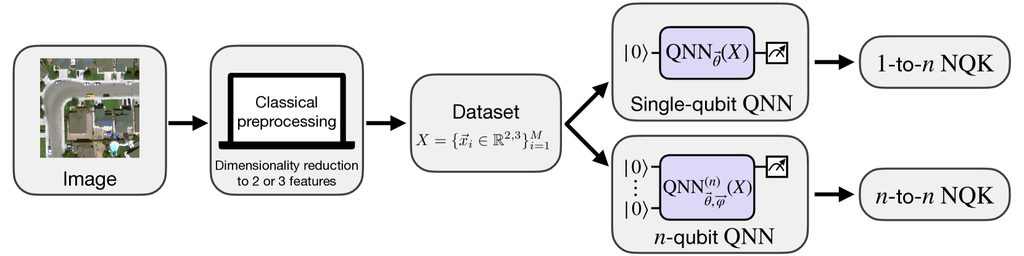
The encoder produces 64-sized vectors as output from the bottleneck dense layer. Depending on the size of the parameterized circuit, these features can be further reduced through dimensionality reduction techniques. The pipeline selected for this problem is displayed in Figure 2. Once the latent features have been obtained, $z$-score normalization is applied to them prior to the application of dimensionality reduction through PCA. The number of components $p$ for PCA is selected as a hyperparameter of the model that depends on the specific requirements of the circuit’s encoding. Before embedding the features into the quantum circuit, their values are scaled to fit within the range of $[-1,1]$. Finally, the circuit yields the prediction $\widehat{y}$, that is either positive class +1 or negative -1.

Figure 4: Detailed NQK construction process. The diagram starts with the training of a single-qubit QNN, from which we obtain the optimal parameters ${\overrightarrow{\theta }}^{\ast }$. Using these parameters, a $1$-to-$n$ NQK can be constructed. The upper part of the figure illustrates the specific case of a $1$-to-$2$ NQK construction. From the trained single-qubit QNN, we can also scale up to construct a 2-qubit QNN, as shown in the lower part of the figure. By iteratively applying this strategy, an $n$-qubit QNN can be constructed and used as the embedding for an $n$-to-$n$ NQK.

IV Methodology

Classical pre-processing serves as a vital step in handling highly intricate real-world datasets. Within our pre-processing framework detailed in Section III.2, PCA stands out as a key technique which inherently introduces nonlinearities to the model. This way, the choice of the number of principal components $p$ becomes a crucial hyperparameter of the model.

In our study, we focus on $p=2$ and $p=3$ features since we are using qubits for the quantum part. Additionally, despite retaining more data information, considering a larger number of principal components does not guarantee improved performance, as our findings will illustrate.

After reducing the data dimensionality, we combine two well-known QML architectures, namely QNNs and EQKs, to create a more robust model termed NQKs.

IV.1 Data re-uploading QNN

We adopt the data re-uploading architecture described in Refs. Pérez-Salinas et al. (2020, 2021) for our QNN. For a single-qubit, this is defined by

$${\mathrm{QNN}}_{\overrightarrow{\theta }}(\overrightarrow{x})\equiv \prod _{l=1}^{L}U({\overrightarrow{\theta }}_l)U(\overrightarrow{x})=U({\overrightarrow{\theta }}_L)U(\overrightarrow{x})\mathrm{\dots }U({\overrightarrow{\theta }}_1)U(\overrightarrow{x}).$$ (2)

This structure alternates parametrized gates $U({\overrightarrow{\theta }}_l)$ with encoding gates $U(\overrightarrow{x})$. Here, $U$ represents a generic $\mathrm{SU}(2)$ unitary, parameterized by three angles. The number of free parameters is $3\times L$, where $L$ denotes the number of layers, contained within the vector $\overrightarrow{\theta }=\{{\overrightarrow{\theta }}_1,\mathrm{\dots },{\overrightarrow{\theta }}_L\}$. Since we are considering data points $\overrightarrow{x}$ with $p=2$ and $p=3$ features, we only need a single encoding unitary. For data points with $p=2$ features, we set the third angle of the encoding gate to 0. This architecture yields highly expressive models, as demonstrated by the analyzed Fourier frequencies of the functions generated by the model Schuld et al. (2021); Casas and Cervera-Lierta (2023). Remarkably, even with a single qubit, one can perform complex classification tasks Tapia et al. (2023); Easom-McCaldin et al. (2024).

The optimal model parameters ${\overrightarrow{\theta }}^{\ast }=\{{\overrightarrow{\theta }}_1^{\ast },\mathrm{\dots },{\overrightarrow{\theta }}_L^{\ast }\}$ are defined as

$${\overrightarrow{\theta }}^{\ast }=\arg \min f_{\mathrm{cost}}(\overrightarrow{\theta }).$$ (3)

The cost function we use is the fidelity cost function

$$f_{\mathrm{cost}}(\overrightarrow{\theta })=\frac{1}{M}\sum _{i=1}^M\left(1-{|⟨{\varphi }_l^i|\varphi (\overrightarrow{\theta },{\overrightarrow{x}}_i)⟩|}^2\right),$$ (4)

where $|{\varphi }_l^i⟩$ denotes the correct label state for data point ${\overrightarrow{x}}_i$ (which are chosen to be either $|0⟩$ or $|1⟩$) and $|\varphi (\overrightarrow{\theta },{\overrightarrow{x}}_i)⟩={\mathrm{QNN}}_{\overrightarrow{\theta }}({\overrightarrow{x}}_i)|0⟩$. Once it is trained, the single-qubit QNN assigns labels according to the decision rule

$$\widehat{y}[{\overrightarrow{x}}_t]=\mathrm{sign}\left(\mathrm{tr}\left(|0⟩⟨0|{\rho }_{{\overrightarrow{\theta }}^{\ast }}({\overrightarrow{x}}_t)\right)-1/2\right)\in \{-1,+1\},$$ (5)

where ${\rho }_{{\overrightarrow{\theta }}^{\ast }}({\overrightarrow{x}}_t)\equiv {\mathrm{QNN}}_{{\overrightarrow{\theta }}^{\ast }}({\overrightarrow{x}}_t)|0⟩⟨0|{\mathrm{QNN}}_{{\overrightarrow{\theta }}^{\ast }}{({\overrightarrow{x}}_t)}^{†}$.

Starting from the single-qubit QNN, we can scale this up by adopting the iterative training strategy outlined in Ref. Rodriguez-Grasa et al. (2024), where the construction of an $n$-qubit QNN proceeds iteratively. This method gradually adds qubits, ensuring that the performance of the $n$-qubit QNN equals or surpasses that of the $(n-1)$-qubit counterpart.

This iterative construction is based on considering a local measurement on the first qubit. Thus, when adding an additional $n$th qubit, if we do so in a way that it is initially decoupled from the previous $n-1$ qubits and initialize the training with the parameters from the previous step, we can ensure that adding this new qubit can only further reduce the value of the cost function. To achieve this decoupling between qubits, all that needs to be done is to initialize the parameters of the controlled rotations that couple the new qubit to the previous ones to 0, resulting in an identity operation.

To implement this strategy, we start by training a single-qubit QNN to determine the optimal parameters ${\overrightarrow{\theta }}^{(1)\ast }$. Subsequently, we expand the network to include a second qubit, constructing the following architecture

$${\mathrm{QNN}}_{\overrightarrow{\theta },\overrightarrow{\phi }}^{(2)}(\overrightarrow{x})=\prod _{l=1}^L\left({\mathrm{CU}}_2^1({\overrightarrow{\phi }}_l^{(1)})\left(U({\overrightarrow{\theta }}_l^{(1)})\otimes U({\overrightarrow{\theta }}_l^{(2)})\right)U{(\overrightarrow{x})}^{\otimes n}\right).$$ (6)

Here, ${\overrightarrow{\theta }}_l^{(1)}$ is initialized with ${\overrightarrow{\theta }}_l^{(1)\ast }$ and ${\overrightarrow{\phi }}_l^{(1)}$ is set to zero for each $l\in [1,L]$ as depicted in Figure 4. Optimization encompasses all parameters, and the optimal values are then used to initialize the $3$-qubit QNN, following the same procedure. Thus, we can scale this up to construct ${\mathrm{QNN}}_{\overrightarrow{\theta },\overrightarrow{\phi }}^{(n)}(\overrightarrow{x})$, where $\overrightarrow{\theta }$ contains all the single-qubit gate trainable parameters and $\overrightarrow{\phi }$ the trainable parameters of the entangling gates.

In this process, the cost function is the same as in Eq. 4, but including now dependency on $\overrightarrow{\phi }$, and the decision rule is expressed as

$$\widehat{y}[{\overrightarrow{x}}_t]=\mathrm{sign}\left(\mathrm{tr}\left(|0⟩⟨0|\otimes {\mathrm{𝟙}}^{(n-1)}{\rho }_{{\overrightarrow{\theta }}^{\ast },{\overrightarrow{\phi }}^{\ast }}^{(n)}({\overrightarrow{x}}_t)\right)-1/2\right),$$ (7)

where ${\rho }_{{\overrightarrow{\theta }}^{\ast },{\overrightarrow{\phi }}^{\ast }}^{(n)}({\overrightarrow{x}}_t)\equiv {\mathrm{QNN}}_{{\overrightarrow{\theta }}^{\ast },{\overrightarrow{\phi }}^{\ast }}^{(n)}({\overrightarrow{x}}_t)|\overrightarrow{0}⟩⟨\overrightarrow{0}|{\mathrm{QNN}}_{{\overrightarrow{\theta }}^{\ast },{\overrightarrow{\phi }}^{\ast }}^{(n)}{({\overrightarrow{x}}_t)}^{†}$, is the quantum state which comes from applying the trained QNN to the $|\overrightarrow{0}⟩$ state.

Figure 5: Numerical results for the $1$-to-$n$ NQKs approach. In $(a)$ and $(b)$, we consider the $1$-to-$2$ NQK, while in $(c)$ we examine the $1$-to-$3$ NQK. The results are displayed for $p=2$ features. The training and test accuracies are drawn from the 10-fold process using the described “$1$-to-$n$ set” of 2000 samples. In the box plots, the upper and lower parts of the boxes represent the 25th and 75th percentiles of the accuracies obtained by evaluating the accuracy of the classifiers using 10-fold. The horizontal line inside the box indicates the median, while the whiskers extend from the box to the most distant evaluation score that lies within 1.5 times the interquartile range (IQR) from the box. Score values beyond the whiskers are considered outliers.

IV.2 Neural quantum kernels

As introduced in Ref. Rodriguez-Grasa et al. (2024), Neural quantum kernels (NQKs) are parameterized EQKs whose parameters are obtained from the training of a QNN. Generally, we denote $n-$to$-n\cdot m$ NQK to signify that a $n-$qubit QNN was used to construct a $n\cdot m-$qubit EQK.

Considering some classical data point $\overrightarrow{x}$ and a quantum embedding $S(\overrightarrow{x})$, EQKs are constructed as follows

$$k({\overrightarrow{x}}_i,{\overrightarrow{x}}_j)={|⟨\overrightarrow{0}|S{({\overrightarrow{x}}_i)}^{†}S({\overrightarrow{x}}_j)|\overrightarrow{0}⟩|}^2,$$ (8)

where $|\overrightarrow{0}⟩={|0⟩}^{\otimes n}$. However, the optimal embedding varies depending on the problem. Therefore, we allow the embedding to be parameterized, defining a parameterized EQK. For NQKs, the embedding parameters are obtained from the training of a QNN.

As depicted in Figure 4, we distinguish between two different NQK architectures: the $1$-to-$n$ and the $n$-to-$n$. In the $1$-to-$n$ approach, a single-qubit QNN is trained, and the obtained parameters are used to construct an $n$-qubit EQK. In the $n$-to-$n$ approach, the single-qubit QNN is scaled to an $n$-qubit QNN, and this architecture is directly used to construct an $n$-qubit EQK. By combining these approaches, one could build the general $n$-to-$n\cdot m$ NQK model.

To construct a $1$-to-$n$ NQK, we proceed as follows: we replicate the data re-uploading QNN structure across the $n$ qubits, using the parameters ${\overrightarrow{\theta }}^{\ast }$ obtained from the QNN training as the arguments for the parameterized unitaries. Between layers, we implement a cascade of CNOT gates between nearest neighbor qubits, though other configurations could also be chosen. The precise expression of such embedding is

$$S_{{\overrightarrow{\theta }}^{\ast }}(\overrightarrow{x})=\prod _{l=1}^L\left(\left(\prod _{s=1}^{n-1}{\mathrm{CNOT}}_s^{s+1}\right)U{({\overrightarrow{\theta }}_l^{\ast })}^{\otimes n}U{({\overrightarrow{x}}_j)}^{\otimes n}\right),$$ (9)

where we use the convention ${\prod }_{i=1}^n{A}_i=A_n\mathrm{\dots }{A}_1$, and in ${\mathrm{CNOT}}_s^{s+1}$, the subscript and the superscript denote the control and the target qubits, respectively. The detailed construction of the embedding for the $1$-to-$2$ case is shown in Figure 4.

On the other hand, the $n$-to-$n$ case requires only taking the trained $n$-qubit QNN directly as the embedding

$$S_{{\overrightarrow{\theta }}^{\ast },{\overrightarrow{\phi }}^{\ast }}(\overrightarrow{x})={\mathrm{QNN}}_{{\overrightarrow{\theta }}^{\ast },{\overrightarrow{\phi }}^{\ast }}^{(n)}(\overrightarrow{x}).$$ (10)

Once the quantum embeddings have been define, we construct the kernel matrix $K$ with entries $k_{ij}=k({\overrightarrow{x}}_i,{\overrightarrow{x}}_j)$. This matrix serves as input for a SVM, which solves a convex optimization problem to find optimal $\overrightarrow{\alpha }$ parameters defining the decision rule

$$\widehat{y}[{\overrightarrow{x}}_t]=\mathrm{sign}\left(\sum _{i=1}^M{\alpha }_i{\widehat{y}}_i\frac{k({\overrightarrow{x}}_t,{\overrightarrow{x}}_i)+1}{2}\right),$$ (11)

where ${\{{\overrightarrow{x}}_i\}}_{i=1}^M$ denotes training points from set $X$.

In the construction of NQKs, training the QNN integrates information about the classification problem into the EQK, resulting in a more robust QML model. Indeed, in the following section, we demonstrate that even a QNN that is not perfectly trained can still effectively determine parameters to construct an NQK that performs remarkably well.

V Numerical results and analysis

Once introducing both, the real-world classification problem and the methodologies, we demonstrate that we can achieve performance levels ranging between 85-90%, which is remarkable given the complexity of the classification task. In the following section, we present numerical results showcasing the performance of the described models. Additionally, we provide a classical benchmark for the classification of this dataset, aiming to be as rigorous as possible in evaluating and comparing the performance of the different models.

For each experiment, a different split of the dataset is used to ensure there is no data leakage:

• U-Net training set: this set of 10,895 images is used just to train the U-Net architecture from scratch to generate the embeddings.

• U-Net test set: this set comprising 6,630 images is used for inference on the U-Net to extract image latent features. This approach ensures that there is no data leakage on the extracted embeddings, since the mask is not used.

• $1$-to-$n$ set: it is a 2000-sample random subset from the U-Net test set to be used in both the $1$-to-$n$ NQK experiments and the classical benchmarking. It is used by performing the stratified 10-fold strategy to get robust test results.

• $n$-to-$n$ set: random subsets from the U-Net test set are selected to perform $n$-to-$n$ NQK experiments. We consider a total of 700 samples, which are divided into 500 training points and 200 test points.

Please refer to Appendix B for further details on the approximation carried out in this work to avoid leakage through dataset splits.

Figure 6: Numerical results for the $n$-to-$n$ architecture, tested using datasets with 500 training points and 200 test points. Experiments were conducted using 2 and 3 features, with results averaged over five independent trials. The “scale QNN set” was utilized for these experiments, as described in the main text. The figure displays the average training and test accuracies for both the QNN and the corresponding $n$-to-$n$ NQK.

V.1 $1$-to-$n$ NQK

For these experiments, we used the “$1$-to-$n$ set” comprising 2000 images. The $k$-fold method was performed with $k=10$ to obtain robust and reliable evaluation metrics. On each of the 10 iterations, 9 folds of the dataset were used for training (1800 images), and 1 fold was used for testing (200 images). This approach yields the results illustrated in Figure 5, which depicts the training and test accuracies for the single-qubit QNN and the NQK. This visualization highlights that models with fewer or no outliers and narrower boxes are more robust, as their performance remains more consistent across different evaluation folds.

We examine both $p=2$ and $p=3$ features but primarily focused on $p=2$, as using three features surprisingly performs less effectively for this classification problem. The results for $p=3$ are presented in Appendix C. For the number of qubits in the EQK, we considered $n=2$ and $n=3$, corresponding to $1$-to-$2$ and $1$-to-$3$ NQKs, respectively. For this classification task, increasing the number of qubits does not enhance performance. Notably, we achieved high classification accuracies even with a small number of qubits.

We distinguish between optimal and sub-optimal QNN training scenarios, both employing an Adam optimizer. For optimal QNN training, the QNN is allowed to converge over 10 epochs with a learning rate of 0.01. In contrast, for sub-optimal QNN training, the process is truncated after 2 epochs to prevent convergence of the loss function, and a lower learning rate of 0.001 was used. This differentiation aims to demonstrate the robustness of NQKs. We observe that while better trained QNNs show minimal improvement from introducing NQK, the NQK’s performance remains high even when the QNN training is suboptimal. This indicates that only a few training iterations are sufficient to select a suitable embedding for constructing a robust NQK. While optimal QNN training is straightforward for systems with few qubits, the robustness of NQK becomes crucial for larger QML models where optimal training is not guaranteed. In such cases, NQKs could be a candidate to circumvent QNN trainability problems.

In analyzing Figure 5, we observe that the best results across the three plots reach close to 90% accuracy, with a mean around 86%. In Figure 5 $(a)$, where the single-qubit QNN is optimally trained, constructing the 2-qubit NQK offers minimal improvement, although the results with NQK are more concentrated. In Figure 5 $(b)$, with sub-optimal QNN training, QNN accuracies drop to around 75-80%, while the 2-qubit NQK performs nearly as well as in the optimal training scenario. Additionally, the wider boxes of the QNN indicate a strong dependency on parameter initialization and the image set used, whereas the narrow NQK boxes demonstrate its robustness. Figure 5 $(c)$, corresponding to the sub-optimal scenario with a 3-qubit EQK, shows results similar to the 2-qubit case but more concentrated around the mean. This may be due to the larger Hilbert space enhancing the linear separation.

V.2 $n$-to-$n$ NQK

In our second approach, instead of constructing an EQK after training a single-qubit QNN, we scale the model up to an $n$-qubit QNN and then derive an $n$-qubit NQK. This scaling is performed iteratively, ensuring that the cost function does not increase when adding qubits, allowing for progressive model improvement.

The results are presented in Figure 6, which shows the mean training and test accuracies along with the standard deviation across 5 independent runs, each using distinct training and test sets. For this analysis, we employed a 6-layer QNN, the Adam optimizer with a learning rate of 0.005, and 10 epochs, scaling the model up to $n=8$ qubits.

The four plots in the figure reveal that accuracies generally increase with the number of qubits, with a more pronounced improvement in training accuracy due to its direct link to the cost function. The standard deviation of test accuracies is naturally larger, reflecting the variability across different subsets.

In Figures 6 $(a)$ and $(b)$, results with $p=2$ features are shown, while Figures 6 $(c)$ and $(d)$ depict the outcomes with $p=3$ features. Overall, the NQK approach consistently outperforms the QNN architecture across all configurations. Specifically, with $p=3$ features, the average training accuracy nears 90%, and the mean test accuracy exceeds 86%. In contrast, with $p=2$ features, the NQK approach achieves average training and test accuracies of over 88% and 84%, respectively. However, slight overfitting is observed, as indicated by the higher training accuracies compared to test accuracies, which is expected given the dataset’s complexity.

V.3 Classical benchmark

Model	$n$ components	Train	Test
SVC	$p=2$	86.1$\pm$0.3	86.2$\pm$2.5
	$p=3$	88.0$\pm$0.3	88.1$\pm$2.7
	$p=45$	89.4$\pm$0.3	89.4$\pm$2.5
Random Forest	$p=2$	91.1$\pm$0.3	87.2$\pm$2.7
	$p=3$	93.0$\pm$0.3	87.6$\pm$2.0
	$p=10$	96.9$\pm$0.2	88.3$\pm$2.8
$1$-to-$2$ NQK	$p=2$	86.6$\pm$0.3	86.5$\pm$2.5
	$p=3$	81.7$\pm$1.8	81.1$\pm$2.9
$1$-to-$3$ NQK	$p=2$	86.6$\pm$0.3	86.5$\pm$2.6
	$p=3$	85.9$\pm$0.6	85.6$\pm$2.7

Table 1: Mean training and test accuracies for two classical classification methods are presented. All experiments employ the same 10-fold setup used in the NQK experiments, with 1800 training points and 200 test points. The results from the NQKs come from the optimal training of the QNNs.

Until now, our investigation has revolved around a hybrid architecture combining classical preprocessing with two distinct QML methodologies. Presently, we delve into classical approaches as substitutes for the quantum components to benchmark our models. In order to accomplish this, we use the preprocessing framework outlined in Section III.2 and then perform the same 10-fold approximation for training and evaluation with classical machine learning algorithms.

The selected models for benchmarking are Support Vector Machine classifier (SVC) and Random Forest classifier. As shown in Table 1, three runs are performed for each model. In order to ensure a fair comparison with the EQK models, the number of features is fixed to $p=2$ and $p=3$ in the first two rows for each model. A hyperparameter optimization with randomized search is then performed to yield nearly optimal test results. In the last row for each model, also $p$ is treated as an hyperparameter in the randomized search to determine if it would yield better results than using $p\in \{2,3\}$. The results of our analysis indicate that the optimal value of $p$ for the SVC is $p=45$, while for the Random Forest it is $p=10$. The values for the remaining hyperparameters for each model can be found in Appendix D.

VI Conclusions

This work addresses a complex binary classification task on a real dataset, focusing on the classification of satellite images to determine whether they contain solar panels or not. Classical preprocessing is conducted to reduce the data dimensionality, employing a cross-task transfer learning implementation, which demonstrates notable effectiveness for this purpose. Once the data dimensionality is reduced to enable processing with quantum models, we utilize two different NQK approaches achieving maximal accuracies near 90%.

We initially explored the $1$-to-$n$ NQK approach. In this model, we observed that constructing an EQK from the training of a single-qubit QNN demonstrates robustness, yielding nearly identical results whether the QNN is optimally or sub-optimally trained. Additionally, we investigated $n$-to-$n$ NQKs, which involve building a scalable $n$-qubit QNN and constructing the corresponding quantum kernel. During the scaling of the QNN, we found that the highest accuracies were achieved by increasing the number of qubits. We also observed robustness in the results when constructing the kernel. With both methods, we successfully match the performance of classical methods, which have also been optimized for the number of features. While the results presented focus on a limited number of qubits, suggesting that the quantum models could be considered quantum-inspired, we demonstrate that, for this classification task, the accuracy values achieved using various quantum and classical methods converge to similar levels.

This work aims to solve a real classification problem with industrial applications using quantum methodology. For this task, we have observed that with a low number of qubits, we can achieve accuracies comparable to the best classical models. However, it would be of great interest to explore tasks that require further scaling of these approaches in terms of the number of qubits. For future considerations, we could assess the performance of this approach on datasets with greater class imbalance and consider implementing it in on noisy quantum simulation backends or actual quantum hardware.

VII Acknowledgements

This work was supported by the Spanish Ministry of Science and Innovation under the Recovery, Transformation and Resilience Plan (CUCO, MIG-20211005). PR and MS acknowledge support from HORIZON-CL4- 2022-QUANTUM01-SGA project 101113946 OpenSuperQPlus100 of the EU Flagship on Quantum Technologies, the Spanish Ramón y Cajal Grant RYC-2020-030503-I, project Grant No. PID2021-125823NA-I00 funded by MCIN/AEI/10.13039/501100011033 and by “ERDF A way of making Europe” and “ERDF Invest in your Future”, and from the IKUR Strategy under the collaboration agreement between Ikerbasque Foundation and BCAM on behalf of the Department of Education of the Basque Government. This project has also received support from the Spanish Ministry of Economic Affairs and Digital Transformation through the QUANTUM ENIA project call - Quantum Spain, and by the EU through the Recovery, Transformation and Resilience Plan - NextGenerationEU. We acknowledge funding from Basque Government through Grant No. IT1470-22 and through the ELKARTEK program, project ”KUBIT - Kuantikaren Berrikuntzarako Ikasketa Teknologikoa” (KK-2024/00105).

Appendix A Modified U-Net architecture

The classical architecture chosen for semantic segmentation purposes was the well-known U-Net Ronneberger et al. (2015) due to its simplicity and adaptability to the PV plants use case. However, the architecture has been slightly modified to extract one-dimensional bottleneck features to be used in classification tasks, as the main goal was not to solve a semantic segmentation problem.

As shown in Figure A.1, the principal changes in the architecture are:

• New added fully-connected layers. At the end of the encoder part of the U-Net, a new $64$-sized fully-connected layer is introduced to be used as the bottleneck layer to extract features later. These new layers have been trained from scratch along with the rest of the architecture, thus transfer learning is not applied in this case.

• Global max pooling and reshaping layers. To adapt the new bottleneck layer, at the end of the last convolutional layer in the encoder, a global max pooling layer is applied to get a one-dimensional output. Following the application of the bottleneck layer, a bidimensional feature map of size $16\times 16$ is reconstructed by adding a 256-sized fully-connected layer and then reshaping its output.

Figure A.1: Modified U-Net architecture used to extract bottleneck features

Appendix B Dataset splits

Dividing a dataset in splits is a mandatory practice in machine learning experiments to ensure rigorous results and to avoid data leakage, as it could lead to overly optimistic performance estimates and poor generalization of the models to new data. When dealing with hybrid models with multiple steps in the pipeline, special care must be taken.

Figure B.1: Dataset splits used for each step of the pipeline

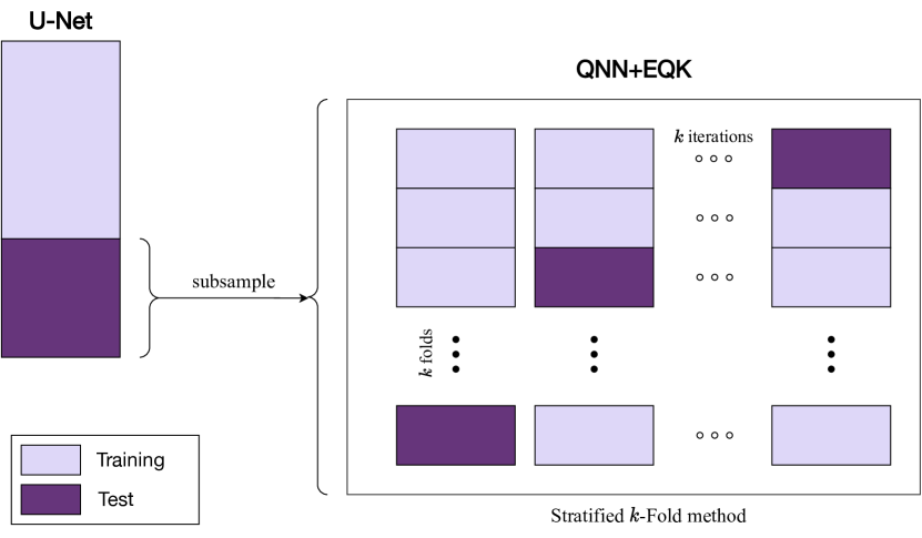
In semantic segmentation, the label is the binary mask. During the training of the U-Net architecture, some of the mask information from the training samples is being fed to the network through backpropagation. Therefore, the U-Net training samples should not be used in later stages for quantum experiments. Figure B.1 illustrates the approximation for this work to avoid such phenomenon.

Appendix C Numerical experiments

Presented here are additional numerical findings not featured in the main text. In Figure C.1, we explore all the NQK construction scenarios, encompassing $p=2$ and $p=3$ features, optimal and sub-optimal QNN training methods, and $n=2$ and $n=3$ qubits. As discussed in the main text, employing $p=2$ features yields superior performance for this architecture and classification task. We can also observe no improvement when transitioning from $n=2$ to $n=3$ qubits in this context.

Figure C.1: Numerical results for the NQK approach: This figure illustrates the outcomes for all combinations involving $p=2$ and $p=3$ features, optimal and sub-optimal training of the QNN component, and $n=2$ and $n=3$ qubits used in kernel construction.

Appendix D Hyperparameters for the classical benchmark

In order to obtain reliable and robust classical results on the dataset to compare with the quantum approaches, a randomized search of the hyperparameters for the selected models (SVC and Random Forest) was performed. It should be noted that the randomised search is not guaranteed to reach the global optimum in the parameter space, but with sufficient iterations it retrieves a satisfactory approximation. The number of iterations set for these experiments was set to 5000.

To ensure a fair comparison, the models were initially tested with the same number of features as the NQK experiments ($p\in \{2,3\}$). Subsequently, the number of components was also set as an hyperparameter on the search, as the original embeddings are of size 64. Tables 2 and 3 present the values of the hyperparameters identified through the randomized search for each model.

In SVM classifiers, the key hyperparameters are kernel, C, and gamma. The kernel function (e.g., linear, polynomial, RBF) transforms input data to find the optimal hyperplane for classification. The C parameter controls the trade-off between low training error and generalization. The gamma parameter, specific to RBF, polynomial, and sigmoid kernels, defines the influence range of a single training example. In the case of Table 2, even though the parameter gamma is optimized, it has no influence, because the optimal selected kernel is linear in all three cases.

Model	n_components	kernel	C	gamma
SVC	$p=2$	linear	9.53	0.016
	$p=3$	linear	10.09	0.079
	$p=45$	linear	10.04	0.085

Table 2: Optimal values for the hyperparameters of the SVC found by the randomized search

In Random Forest classifiers, some of the key hyperparameters are n_estimators, max_depth, and max_features. The n_estimators parameter specifies the number of trees in the forest, where more trees generally improve performance but increase computational cost. The max_depth parameter controls the maximum depth of each tree, preventing overfitting by limiting how deep the trees can grow. The max_features parameter determines the number of features to consider when looking for the best split, balancing between the model’s accuracy and computational efficiency.

Model	n_components	n_estimators	max_depth	max_features
Random Forest	$p=2$	72	40	sqrt
	$p=3$	197	96	sqrt
	$p=10$	103	13	sqrt

Table 3: Optimal values for the hyperparameters of the Random Forest classifier found by the randomized search

In order to ensure the reproducibility of the results, all of these classical experiments have been conducted using the scikit-learn Python library.

References

- Biamonte et al. (2017) Jacob Biamonte, Peter Wittek, Nicola Pancotti, Patrick Rebentrost, Nathan Wiebe, and Seth Lloyd, “Quantum machine learning,” Nature 549, 195–202 (2017).
- Carleo et al. (2019) Giuseppe Carleo, Ignacio Cirac, Kyle Cranmer, Laurent Daudet, Maria Schuld, Naftali Tishby, Leslie Vogt-Maranto, and Lenka Zdeborová, “Machine learning and the physical sciences,” Rev. Mod. Phys. 91, 045002 (2019).
- Dunjko and Briegel (2018) Vedran Dunjko and Hans J Briegel, “Machine learning & artificial intelligence in the quantum domain: a review of recent progress,” Reports on Progress in Physics 81, 074001 (2018).
- Huang et al. (2021a) Hsin-Yuan Huang, Michael Broughton, Masoud Mohseni, Ryan Babbush, Sergio Boixo, Hartmut Neven, and Jarrod R. McClean, “Power of data in quantum machine learning,” Nature Communications 12, 2631 (2021a).
- Schuld (2021) Maria Schuld, “Supervised quantum machine learning models are kernel methods,” (2021), arXiv:2101.11020 [quant-ph] .
- Jerbi et al. (2023) Sofiene Jerbi, Lukas J. Fiderer, Hendrik Poulsen Nautrup, Jonas M. Kübler, Hans J. Briegel, and Vedran Dunjko, “Quantum machine learning beyond kernel methods,” Nature Communications 14, 517 (2023).
- Schuld and Killoran (2019) Maria Schuld and Nathan Killoran, “Quantum machine learning in feature hilbert spaces,” Phys. Rev. Lett. 122, 040504 (2019).
- McClean et al. (2018) Jarrod R. McClean, Sergio Boixo, Vadim N. Smelyanskiy, Ryan Babbush, and Hartmut Neven, “Barren plateaus in quantum neural network training landscapes,” Nature Communications 9, 4812 (2018).
- Cerezo et al. (2021) M. Cerezo, Akira Sone, Tyler Volkoff, Lukasz Cincio, and Patrick J. Coles, “Cost function dependent barren plateaus in shallow parametrized quantum circuits,” Nature Communications 12, 1791 (2021).
- Holmes et al. (2022) Zoë Holmes, Kunal Sharma, M. Cerezo, and Patrick J. Coles, “Connecting ansatz expressibility to gradient magnitudes and barren plateaus,” PRX Quantum 3, 010313 (2022).
- Fontana et al. (2024) Enrico Fontana, Dylan Herman, Shouvanik Chakrabarti, Niraj Kumar, Romina Yalovetzky, Jamie Heredge, Shree Hari Sureshbabu, and Marco Pistoia, “The adjoint is all you need: Characterizing barren plateaus in quantum ansätze,” (2024), arXiv:2309.07902 [quant-ph] .
- Ragone et al. (2023) Michael Ragone, Bojko N. Bakalov, Frédéric Sauvage, Alexander F. Kemper, Carlos Ortiz Marrero, Martin Larocca, and M. Cerezo, “A unified theory of barren plateaus for deep parametrized quantum circuits,” (2023), arXiv:2309.09342 [quant-ph] .
- Thanasilp et al. (2024) Supanut Thanasilp, Samson Wang, M. Cerezo, and Zoë Holmes, “Exponential concentration in quantum kernel methods,” (2024), arXiv:2208.11060 [quant-ph] .
- Pesah et al. (2021) Arthur Pesah, M. Cerezo, Samson Wang, Tyler Volkoff, Andrew T. Sornborger, and Patrick J. Coles, “Absence of barren plateaus in quantum convolutional neural networks,” Phys. Rev. X 11, 041011 (2021).
- Caro et al. (2021) Matthias C. Caro, Elies Gil-Fuster, Johannes Jakob Meyer, Jens Eisert, and Ryan Sweke, “Encoding-dependent generalization bounds for parametrized quantum circuits,” Quantum 5, 582 (2021).
- Caro et al. (2022) Matthias C. Caro, Hsin-Yuan Huang, M. Cerezo, Kunal Sharma, Andrew Sornborger, Lukasz Cincio, and Patrick J. Coles, “Generalization in quantum machine learning from few training data,” Nature Communications 13, 4919 (2022).
- Peters and Schuld (2023) Evan Peters and Maria Schuld, “Generalization despite overfitting in quantum machine learning models,” Quantum 7, 1210 (2023).
- Banchi et al. (2021) Leonardo Banchi, Jason Pereira, and Stefano Pirandola, “Generalization in quantum machine learning: A quantum information standpoint,” PRX Quantum 2, 040321 (2021).
- Gil-Fuster et al. (2024) Elies Gil-Fuster, Jens Eisert, and Carlos Bravo-Prieto, “Understanding quantum machine learning also requires rethinking generalization,” Nature Communications 15, 2277 (2024).
- Gyurik and Dunjko (2023) Casper Gyurik and Vedran Dunjko, “On establishing learning separations between classical and quantum machine learning with classical data,” (2023), arXiv:2208.06339 [quant-ph] .
- Sweke et al. (2021) Ryan Sweke, Jean-Pierre Seifert, Dominik Hangleiter, and Jens Eisert, “On the Quantum versus Classical Learnability of Discrete Distributions,” Quantum 5, 417 (2021).
- Jerbi et al. (2021) Sofiene Jerbi, Lea M. Trenkwalder, Hendrik Poulsen Nautrup, Hans J. Briegel, and Vedran Dunjko, “Quantum enhancements for deep reinforcement learning in large spaces,” PRX Quantum 2, 010328 (2021).
- Liu et al. (2021) Yunchao Liu, Srinivasan Arunachalam, and Kristan Temme, “A rigorous and robust quantum speed-up in supervised machine learning,” Nature Physics 17, 1013–1017 (2021).
- Pirnay et al. (2023) Niklas Pirnay, Ryan Sweke, Jens Eisert, and Jean-Pierre Seifert, “Superpolynomial quantum-classical separation for density modeling,” Phys. Rev. A 107, 042416 (2023), arXiv:2210.14936 [quant-ph] .
- Havlíček et al. (2019) Vojtěch Havlíček, Antonio D. Córcoles, Kristan Temme, Aram W. Harrow, Abhinav Kandala, Jerry M. Chow, and Jay M. Gambetta, “Supervised learning with quantum-enhanced feature spaces,” Nature 567, 209–212 (2019).
- Johri et al. (2021) Sonika Johri, Shantanu Debnath, Avinash Mocherla, Alexandros SINGK, Anupam Prakash, Jungsang Kim, and Iordanis Kerenidis, “Nearest centroid classification on a trapped ion quantum computer,” npj Quantum Information 7, 122 (2021).
- Ristè et al. (2017) Diego Ristè, Marcus P. da Silva, Colm A. Ryan, Andrew W. Cross, Antonio D. Córcoles, John A. Smolin, Jay M. Gambetta, Jerry M. Chow, and Blake R. Johnson, “Demonstration of quantum advantage in machine learning,” npj Quantum Information 3, 16 (2017).
- Steinbrecher et al. (2019) Gregory R. Steinbrecher, Jonathan P. Olson, Dirk Englund, and Jacques Carolan, “Quantum optical neural networks,” npj Quantum Information 5, 60 (2019).
- Peters et al. (2021) Evan Peters, João Caldeira, Alan Ho, Stefan Leichenauer, Masoud Mohseni, Hartmut Neven, Panagiotis Spentzouris, Doug Strain, and Gabriel N Perdue, “Machine learning of high dimensional data on a noisy quantum processor,” npj Quantum Information 7, 161 (2021).
- Jadhav et al. (2023) Abhishek Jadhav, Akhtar Rasool, and Manasi Gyanchandani, “Quantum machine learning: Scope for real-world problems,” Procedia Computer Science 218, 2612–2625 (2023), international Conference on Machine Learning and Data Engineering.
- Matic et al. (2022) Andrea Matic, Maureen Monnet, Jeanette Miriam Lorenz, Balthasar Schachtner, and Thomas Messerer, “Quantum-classical convolutional neural networks in radiological image classification,” (2022), arXiv:2204.12390 [quant-ph] .
- Henderson et al. (2020a) Maxwell Henderson, Samriddhi Shakya, Shashindra Pradhan, and Tristan Cook, “Quanvolutional neural networks: powering image recognition with quantum circuits,” Quantum Machine Intelligence 2, 2 (2020a).
- Lü et al. (2021) Yanxuan Lü, Qing Gao, Jinhu Lü, Maciej Ogorzałek, and Jin Zheng, “A quantum convolutional neural network for image classification,” in 2021 40th Chinese Control Conference (CCC) (2021) pp. 6329–6334.
- Chen et al. (2023) Guoming Chen, Qiang Chen, Shun Long, Weiheng Zhu, Zeduo Yuan, and Yilin Wu, “Quantum convolutional neural network for image classification,” Pattern Analysis and Applications 26, 655–667 (2023).
- Chang et al. (2023) Su Yeon Chang, Michele Grossi, Bertrand Le Saux, and Sofia Vallecorsa, “Approximately equivariant quantum neural network for p4m group symmetries in images,” in 2023 IEEE International Conference on Quantum Computing and Engineering (QCE) (IEEE, 2023).
- West et al. (2023) Maxwell T West, Martin Sevior, and Muhammad Usman, “Reflection equivariant quantum neural networks for enhanced image classification,” Machine Learning: Science and Technology 4, 035027 (2023).
- Sebastian et al. (2024) Paul San Sebastian, Mikel Cañizo, and Román Orús, “Image classification with rotation-invariant variational quantum circuits,” (2024), arXiv:2403.15031 [quant-ph] .
- West et al. (2024) Maxwell T. West, Jamie Heredge, Martin Sevior, and Muhammad Usman, “Provably trainable rotationally equivariant quantum machine learning,” (2024), arXiv:2311.05873 [quant-ph] .
- Senokosov et al. (2024) Arsenii Senokosov, Alexandr Sedykh, Asel Sagingalieva, Basil Kyriacou, and Alexey Melnikov, “Quantum machine learning for image classification,” Machine Learning: Science and Technology 5, 015040 (2024).
- Dang et al. (2018) Yijie Dang, Nan Jiang, Hao Hu, Zhuoxiao Ji, and Wenyin Zhang, “Image classification based on quantum k-nearest-neighbor algorithm,” Quantum Information Processing 17, 239 (2018).
- (41) European Space Agency (ESA), “Satellite Missions catalogue,” https://www.eoportal.org/satellite-missions?Mission+type=EO.
- Commission (2018) European Commission, “The DIAS: User-friendly Access to Copernicus Data and Information,” https://www.copernicus.eu/sites/default/files/Copernicus_DIAS_Factsheet_June2018.pdf (2018).
- Zollner et al. (2024) Johann Zollner, Paul Walther, and Martin Werner, “Satellite image representations for quantum classifiers,” Datenbank-Spektrum 24 (2024), 10.1007/s13222-024-00464-7.
- Sebastianelli et al. (2022) Alessandro Sebastianelli, Daniela Alessandra Zaidenberg, Dario Spiller, Bertrand Le Saux, and Silvia Liberata Ullo, “On circuit-based hybrid quantum neural networks for remote sensing imagery classification,” IEEE Journal of Selected Topics in Applied Earth Observations and Remote Sensing 15, 565–580 (2022).
- Benítez-Buenache and Portell-Montserrat (2024) Alexander Benítez-Buenache and Queralt Portell-Montserrat, “Bayesian Parameterized Quantum Circuit Optimization (BPQCO): A task and hardware-dependent approach,” (2024), arXiv:2404.11253 [quant-ph] .
- Mountrakis et al. (2011) Giorgos Mountrakis, Jungho Im, and Caesar Ogole, “Support vector machines in remote sensing: A review,” ISPRS Journal of Photogrammetry and Remote Sensing 66, 247–259 (2011).
- Delilbasic et al. (2021a) Amer Delilbasic, Gabriele Cavallaro, Madita Willsch, Farid Melgani, Morris Riedel, and Kristel Michielsen, “Quantum Support Vector Machine Algorithms for Remote Sensing Data Classification,” in 2021 IEEE International Geoscience and Remote Sensing Symposium IGARSS (2021) pp. 2608–2611.
- Bradbury et al. (2016) Kyle Bradbury, Raghav Saboo, Timothy Johnson, Jordan Malof, Arjun Devarajan, Wuming Zhang, Leslie Collins, and Richard Newell, “Distributed solar photovoltaic array location and extent dataset for remote sensing object identification,” Scientific Data 3, 160106 (2016).
- Preskill (2018) John Preskill, “Quantum Computing in the NISQ era and beyond,” Quantum 2, 79 (2018).
- Rodriguez-Grasa et al. (2024) Pablo Rodriguez-Grasa, Yue Ban, and Mikel Sanz, “Training embedding quantum kernels with data re-uploading quantum neural networks,” (2024), arXiv:2401.04642 [quant-ph] .
- Otgonbaatar and Datcu (2022) Soronzonbold Otgonbaatar and Mihai Datcu, “Classification of remote sensing images with parameterized quantum gates,” IEEE Geoscience and Remote Sensing Letters 19, 1–5 (2022).
- Helber et al. (2019) Patrick Helber, Benjamin Bischke, Andreas Dengel, and Damian Borth, “Eurosat: A novel dataset and deep learning benchmark for land use and land cover classification,” (2019), arXiv:1709.00029 [cs.CV] .
- Henderson et al. (2020b) Maxwell Henderson, Jarred Gallina, and Michael Brett, “Methods for accelerating geospatial data processing using quantum computers,” (2020b), arXiv:2004.03079 [quant-ph] .
- Basu et al. (2015) Saikat Basu, Sangram Ganguly, Supratik Mukhopadhyay, Robert DiBiano, Manohar Karki, and Ramakrishna Nemani, “Deepsat: a learning framework for satellite imagery,” in Proceedings of the 23rd SIGSPATIAL International Conference on Advances in Geographic Information Systems, SIGSPATIAL ’15 (Association for Computing Machinery, New York, NY, USA, 2015).
- Zaidenberg et al. (2021) Daniela A. Zaidenberg, Alessandro Sebastianelli, Dario Spiller, Bertrand Le Saux, and Silvia Liberata Ullo, “Advantages and bottlenecks of quantum machine learning for remote sensing,” in 2021 IEEE International Geoscience and Remote Sensing Symposium IGARSS (2021) pp. 5680–5683.
- Daudt et al. (2018) Rodrigo Caye Daudt, B. L. Saux, Alexandre Boulch, and Yann Gousseau, “Urban change detection for multispectral earth observation using convolutional neural networks,” IGARSS 2018 - 2018 IEEE International Geoscience and Remote Sensing Symposium , 2115–2118 (2018).
- Otgonbaatar et al. (2023) Soronzonbold Otgonbaatar, Gottfried Schwarz, Mihai Datcu, and Dieter Kranzlmüller, “Quantum transfer learning for real-world, small, and high-dimensional remotely sensed datasets,” IEEE Journal of Selected Topics in Applied Earth Observations and Remote Sensing 16, 9223–9230 (2023).
- Sebastianelli et al. (2023) Alessandro Sebastianelli, Maria Pia Del Rosso, Silvia Liberata Ullo, and Paolo Gamba, “On quantum hyperparameters selection in hybrid classifiers for earth observation data,” IEEE Geoscience and Remote Sensing Letters 20, 1–5 (2023).
- Delilbasic et al. (2021b) Amer Delilbasic, Gabriele Cavallaro, Madita Willsch, Farid Melgani, Morris Riedel, and Kristel Michielsen, “Quantum support vector machine algorithms for remote sensing data classification,” in 2021 IEEE International Geoscience and Remote Sensing Symposium IGARSS (2021) pp. 2608–2611.
- Centre. (2023) European Commission. Joint Research Centre., Quantum Machine Learning for Remote Sensing: Exploring potential and challenges (Publications Office, 2023).
- Erdener et al. (2022) Burcin Cakir Erdener, Cong Feng, Kate Doubleday, Anthony Florita, and Bri-Mathias Hodge, “A review of behind-the-meter solar forecasting,” Renewable and Sustainable Energy Reviews 160, 112224 (2022).
- Feng et al. (2021) Cong Feng, Yuanzhi Liu, and Jie Zhang, “A taxonomical review on recent artificial intelligence applications to pv integration into power grids,” International Journal of Electrical Power & Energy Systems 132, 107176 (2021).
- Yu et al. (2018) Jiafan Yu, Zhecheng Wang, Arun Majumdar, and Ram Rajagopal, “Deepsolar: A machine learning framework to efficiently construct a solar deployment database in the united states,” Joule 2, 2605–2617 (2018).
- Ryu et al. (2020) Seunghyoung Ryu, Hyungeun Choi, Hyoseop Lee, and Hongseok Kim, “Convolutional autoencoder based feature extraction and clustering for customer load analysis,” IEEE Transactions on Power Systems 35, 1048–1060 (2020).
- Ronneberger et al. (2015) Olaf Ronneberger, Philipp Fischer, and Thomas Brox, “U-net: Convolutional networks for biomedical image segmentation,” (2015), arXiv:1505.04597 [cs.CV] .
- Huang et al. (2021b) Bingsheng Huang, Junru Tian, Hongyuan Zhang, Zixin Luo, Jing Qin, Chen Huang, Xueping He, Yanji Luo, Yongjin Zhou, Guo Dan, Hanwei Chen, Shi-Ting Feng, and Chenglang Yuan, “Deep semantic segmentation feature-based radiomics for the classification tasks in medical image analysis,” IEEE Journal of Biomedical and Health Informatics 25, 2655–2664 (2021b).
- Pérez-Salinas et al. (2020) Adrián Pérez-Salinas, Alba Cervera-Lierta, Elies Gil-Fuster, and José I. Latorre, “Data re-uploading for a universal quantum classifier,” Quantum 4, 226 (2020).
- Pérez-Salinas et al. (2021) Adrián Pérez-Salinas, David López-Núñez, Artur García-Sáez, P. Forn-Díaz, and José I. Latorre, “One qubit as a universal approximant,” Physical Review A 104 (2021), 10.1103/physreva.104.012405.
- Schuld et al. (2021) Maria Schuld, Ryan Sweke, and Johannes Jakob Meyer, “Effect of data encoding on the expressive power of variational quantum-machine-learning models,” Phys. Rev. A 103, 032430 (2021).
- Casas and Cervera-Lierta (2023) Berta Casas and Alba Cervera-Lierta, “Multidimensional fourier series with quantum circuits,” Phys. Rev. A 107, 062612 (2023).
- Tapia et al. (2023) Elena Peña Tapia, Giannicola Scarpa, and Alejandro Pozas-Kerstjens, “A didactic approach to quantum machine learning with a single qubit,” Physica Scripta 98, 054001 (2023).
- Easom-McCaldin et al. (2024) Philip Easom-McCaldin, Ahmed Bouridane, Ammar Belatreche, Richard Jiang, and Somaya Al-Maadeed, “Efficient quantum image classification using single qubit encoding,” IEEE Transactions on Neural Networks and Learning Systems 35, 1472–1486 (2024).