Chapter 3. Linear Regression
In this chapter, we will begin applying all the standard steps employed in a machine learning project in order to fit previously given data with a line that minimizes error and loss functions.
In the previous chapter, we saw problems with both a limited scope and a number of possible solutions. These types of models are also related with a qualitative assessment type, that is, assigning a label to a sample, based on previous labeling. This result is normally found in problems pertaining to the social domain.
We could also be interested in predicting the exact numeric output value of a (previously modeled) function. This approach is akin to the physical domain and can be used to predict the temperature or humidity or the value of a certain good, knowing a series of its historical values before hand, and it is called regression analysis.
In the case of linear regression, we look for a determinate relationship between the input and the output variables, represented by a linear equation.
Univariate linear modelling function
As previously stated, in linear regression, we try to find a linear equation that minimizes the distance between data points and the modeled line.
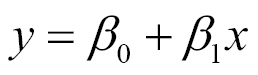
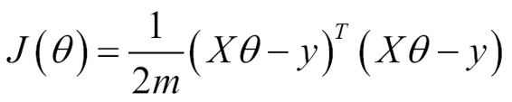
This relationship can be represented by this canonical linear function:
The model function takes the form:
Here, ss0 or bias is the intercept, the function value for x is zero, and ss1 is the slope of the modeled line. The variable x is normally called the independent variable, and y the dependent one, but they can also be called the regressor and response variables respectively.
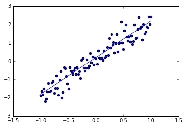
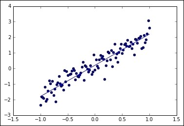
In the following example, we will generate an approximate sample random distribution based on a line with ss0 = 2.0, summed with a vertical noise of maximum amplitude 0.4.
In[]:
#Indicate the matplotlib to show the graphics inline
%matplotlib inline
import matplotlib.pyplot as plt # import matplotlib
import numpy as np # import numpy
trX = np.linspace(-1, 1, 101) # Linear space of 101 and [-1,1]
#Create The y function based on the x axis
trY = 2 * trX + np.random.randn(*trX.shape) * 0.4 + 0.2
plt.figure() # Create a new figure
plt.scatter(trX,trY) #Plot a scatter draw of the random datapoints
# Draw one line with the line function
plt.plot (trX, .2 + 2 * trX)
And the resulting graph will look like this:
Noise added linear sampling and linear function
Determination of the cost function
As with all machine learning techniques, we have to determine an error function, which we need to minimize, that indicates the appropriateness of the solution to the problem.
The most generally used cost function for linear regression is called least squares.
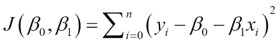
In order to calculate the least squares error for a function, we look for a measure of how close the points are to the modeling line, in a general sense. So we define a function that measures for each tuple xn, yn how far it is from the modeled line's corresponding value.
For 2D regression, we have a list of number tuples (X0,Y0),(X1,Y1)...(Xn,Yn), and the values to find are of β0 and β1, by minimizing the following function:
In simple terms, the summation represents the sum of Euclidean distances between predicted and actual values.
The reason for the operations is that the summation of the squared errors gives us a unique and simple global number, the difference between expected and real number gives us the proper distance, and the square power gives us a positive number, which penalizes distances in a more-than-linear fashion.
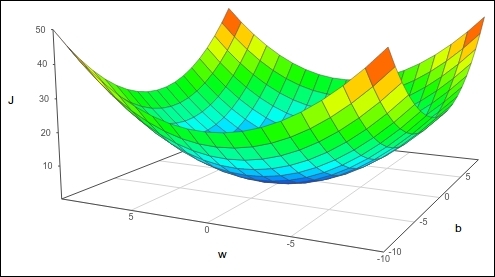
Minimizing the cost function
The next step is to set a method to minimize the cost function. In linear calculus, one of the fundamental elements of the task of locating minima is reduced to calculating the derivatives of the function and to seek its zeroes. For this, the function has to have a derivative and preferably be convex; it can be proved that the least squares function complies with these two conditions. This is very useful for avoiding the known problems of local minima.
Loss function representation
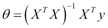
General minima for least squares
The kind of problem we are trying to solve (least squares) can be presented in matrix form:
Here, J is the cost function and has the following solution:
In this chapter, we will use an iterative method gradient descent, which will be useful in the following chapters in a more generalized fashion.
Iterative methods - gradient descent
The gradient descent is by its own nature an iterative method and the most generally used optimization algorithm in the machine learning field. It combines a simple approach with a good convergence rate, considering the complexity of parameter combinations that it can be optimized with it.
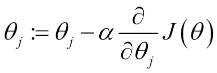
A 2D linear regression starts with a function with randomly defined weights or multipliers for the linear coefficient. After the first values are defined, the second step is to apply a recurrent function in the following form:
In this equation, we can easily derive the mechanism of the method. We start with the initial set of coefficients and then move in the opposite direction of maximum change in the function. The α variable is named the step and will affect how far we will move in the direction of the gradient searching for minimal.
The final step is to optionally test the changes between iteration and see whether the changes are greater than an epsilon or to check whether the iteration number is reached.
If the function is not convex, it is suggested to run gradient descent multiple times with random values and then select coefficients for which the cost value is the lowest. In the case of non-convex functions, the gradient descent ends up in a minimum, which can be local. Therefore, as for non-convex functions, the result depends on initial values, it is suggested to randomly set them multiple times and among all the solutions, pick the one with lowest cost.
Let's now discuss useful libraries and modules.
Optimizer methods in TensorFlow - the train module
The training or parameter optimization stage is a vital part of the machine learning workflow.
For this matter, TensorFlow has a tf.train module, which is a helper set of objects dedicated to implementing a range of different optimizing strategies that the data scientist will need. The main object provided by this module is called Optimizer.
The tf.train.Optimizer class
The Optimizer class allows you to calculate gradients for a loss function and apply them to different variables of a model. Among the most well-known algorithm subclasses, we find gradient descent, Adam, and Adagrad.
One major tip regarding this class is that the Optimizer class itself cannot be instantiated; one of the subclasses should be.
As discussed previously, TensorFlow allows you to define the functions in a symbolic way, so the gradients will be applied in a symbolic fashion, too, improving the accuracy of the results and the versatility of the operations to be applied to the data.
In order to use the Optimizer class, we need to perform the following steps:
- Create an
Optimizer with the desired parameters (in this case, gradient descent). opt = GradientDescentOptimizer(learning_rate= [learning rate])
- Create an operation calling the
minimize method for the cost functions. optimization_op = opt.minimize(cost, var_list=[variables list])
The minimize method has the following form:
tf.train.Optimizer.minimize(loss, global_step=None, var_list=None, gate_gradients=1, aggregation_method=None, colocate_gradients_with_ops=False, name=None)
The main parameters are as follows:
loss: This is a tensor that contains the values to be minimized.global_step: This variable will increment by one after the Optimizer works.var_list: This contains variables to optimize.
Other Optimizer instance types
Following are the other Optimizer instance types:
tf.train.AdagradOptimizer: This is an adaptive method based on the frequency of parameters, with a monotonically descending learning rate.tf.train.AdadeltaOptimizer: This is an improvement on Adagrad, that doesn't carry a descending learning rate.tf.train.MomentumOptimizer: This is an adaptive method that accounts for different change rates between dimensions.- And there are other more specific ones, such as
tf.train.AdamOptimizer, tf.train.FtrlOptimizer, tf.train.RMSPropOptimizer.
Example 1 - univariate linear regression
We will now work on a project in which we will apply all the concepts we succinctly covered in the preceding pages. In this example, we will create one approximately linear distribution; afterwards, we will create a regression model that tries to fit a linear function that minimizes the error function (defined by least squares).
This model will allow us to predict an outcome for an input value, given one new sample.
For this example, we will be generating a synthetic dataset consisting of a linear function with added noise:
import TensorFlow as tf
import numpy as np
trX = np.linspace(-1, 1, 101)
trY = 2 * trX + np.random.randn(*trX.shape) * 0.4 + 0.2 # create a y value which is approximately linear but with some random noise
With these lines, we can represent the lines as a scatter plot and the ideal line function.
import matplotlib.pyplot as plt
plt.scatter(trX,trY)
plt.plot (trX, .2 + 2 * trX)
Generated samples and original linear function without noise
- Now we create a variable to hold the values in the
x and y axes. Then we symbolically define the model as the multiplication of X and the weights w.
- Then we generate some variables, to which we assign initial values in order to launch the model:
        In[]:
        X = tf.placeholder("float", name="X") # create symbolic variables
        Y = tf.placeholder("float", name = "Y")
- We now define our model by declaring
name_scope as Model. This scope groups all the variables it contains in order to form a unique entity with homogeneous entities. In this scope, we first define a function that receives the variables of the x axis coordinates, the weight (slope), and the bias. Then we create a new variable, objects, to hold the changing parameters and instantiate the model with the y_model variable: with tf.name_scope("Model"):
def model(X, w, b):
return tf.mul(X, w) + b # just define the line as X*w + b0
w = tf.Variable(-1.0, name="b0") # create a shared variable
b = tf.Variable(-2.0, name="b1") # create a shared variable
y_model = model(X, w, b)
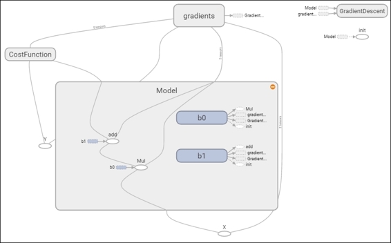
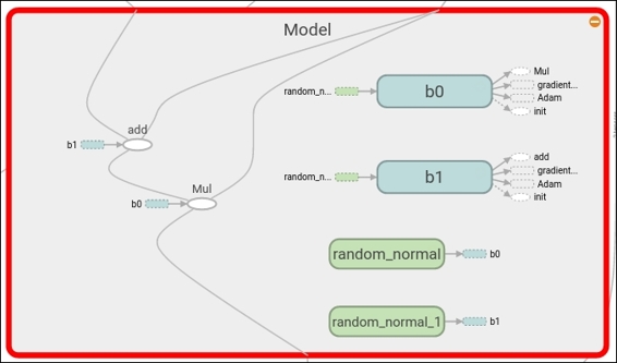
In the dashboard, you can see the image of the loss function we have been recollecting. In the graph section, when you zoom into the Model, you can see the sum and multiplication operation, the parameter variables b0 and b1, and the gradient operation applied over the Model, as shown next:
Cost function description and Optimizer loop
- In the
Cost Function, we create a new scope to include all the operations of this group and use the previously created y_model to account for the calculated y axis values that we use to calculate the loss. with tf.name_scope("CostFunction"):
cost = (tf.pow(Y-y_model, 2)) # use sqr error for cost
- To define the chosen
optimizer, we initialize a GradientDescentOptimizer, and the step will be of 0.01, which seems like a reasonable start for convergence. train_op = tf.train.GradientDescentOptimizer(0.05).minimize(cost)
- It's time to create the session and to initialize the variables we want to save for reviewing in TensorBoard. In this example, we will be saving one scalar variable with the error result of the last sample for each iteration. We will also save the graph structure in a file for reviewing.
        sess = tf.Session()
        init = tf.initialize_all_variables()
        tf.train.write_graph(sess.graph,
          '/home/ubuntu/linear','graph.pbtxt')
        cost_op = tf.scalar_summary("loss", cost)
        merged = tf.merge_all_summaries()
        sess.run(init)
        writer = tf.train.SummaryWriter('/home/ubuntu/linear',
          sess.graph)
- For model training, we set an objective of 100 iterations, where we send each of the samples to the
train operation of the gradient descent. After each iteration, we plot the modeling line and add the value of the last error to the summary. In[]:
for i in range(100):
for (x, y) in zip(trX, trY):
sess.run(train_op, feed_dict={X: x, Y: y})
summary_str = sess.run(cost_op, feed_dict={X: x, Y: y})
writer.add_summary(summary_str, i)
b0temp=b.eval(session=sess)
b1temp=w.eval(session=sess)
plt.plot (trX, b0temp + b1temp * trX )
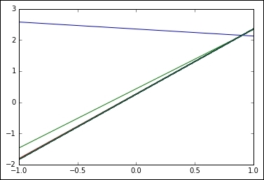
The resulting plot is as follows; we can see how the initial line rapidly converges into a more plausible result:
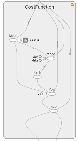
With the CostFunction scope zoomed in, we can see the power and subtraction operations and also the written summary, as shown in the following figure:
Now let's check the parameter results, printing the run output of the w and b variables:
printsess.run(w) # Should be around 2
printsess.run(b) #Should be around 0.2
2.09422
0.256044
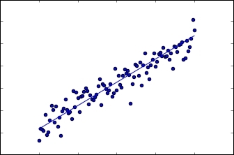
It's time to graphically review the data again and the suggested final line.
plt.scatter(trX,trY)
plt.plot (trX, testb + trX * testw)
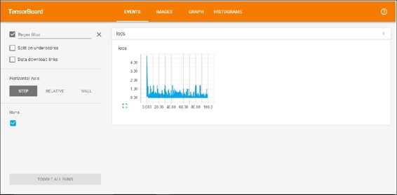
Reviewing results with TensorBoard
Now let's review the data we saved in TensorBoard.
In order to start TensorBoard, you can go to the logs directory and execute the following line:
$ tensorboard --logdir=.
TensorBoard will load the event and graph files and will be listening on the 6006 port. You can then go from your browser to localhost:6000 and see the TensorBoard dashboard as shown in the following figure:
The following is the complete source code:
import matplotlib.pyplot as plt # import matplotlib
import numpy as np # import numpy
import tensorflow as tf
import numpy as np

trX = np.linspace(-1, 1, 101) #Create a linear space of 101 points between 1 and 1
trY = 2 * trX + np.random.randn(*trX.shape) * 0.4 + 0.2 #Create The y function based on the x axis
plt.figure() # Create a new figure
plt.scatter(trX,trY) #Plot a scatter draw of the random datapoints
plt.plot (trX, .2 + 2 * trX) # Draw one line with the line function

get_ipython().magic(u'matplotlib inline')

import matplotlib.pyplot as plt
import tensorflow as tf
import numpy as np

trX = np.linspace(-1, 1, 101)
trY = 2 * trX + np.random.randn(*trX.shape) * 0.4 + 0.2 # create a y value which is approximately linear but with some random noise

plt.scatter(trX,trY)
plt.plot (trX, .2 + 2 * trX)

X = tf.placeholder("float", name="X") # create symbolic variables
Y = tf.placeholder("float", name = "Y")

withtf.name_scope("Model"):

    def model(X, w, b):
        returntf.mul(X, w) + b # We just define the line as X*w + b0

    w = tf.Variable(-1.0, name="b0") # create a shared variable
    b = tf.Variable(-2.0, name="b1") # create a shared variable
    y_model = model(X, w, b)


withtf.name_scope("CostFunction"):
    cost = (tf.pow(Y-y_model, 2)) # use sqr error for cost function

train_op = tf.train.GradientDescentOptimizer(0.05).minimize(cost)


sess = tf.Session()
init = tf.initialize_all_variables()
tf.train.write_graph(sess.graph, '/home/ubuntu/linear','graph.pbtxt')
cost_op = tf.scalar_summary("loss", cost)
merged = tf.merge_all_summaries()
sess.run(init)
writer = tf.train.SummaryWriter('/home/ubuntu/linear', sess.graph)

fori in range(100):
for (x, y) in zip(trX, trY):
sess.run(train_op, feed_dict={X: x, Y: y})
summary_str = sess.run(cost_op, feed_dict={X: x, Y: y})
writer.add_summary(summary_str, i)
    b0temp=b.eval(session=sess)
    b1temp=w.eval(session=sess)
plt.plot (trX, b0temp + b1temp * trX )


printsess.run(w) # Should be around 2
printsess.run(b) #Should be around 0.2


plt.scatter(trX,trY)
plt.plot (trX, sess.run(b) + trX * sess.run(w))
Example - multivariate linear regression
In this example, we will work on a regression problem involving more than one variable.
This will be based on a 1993 dataset of a study of different prices among some suburbs of Boston. It originally contained 13 variables and the mean price of the properties there.
The only change in the file from the original one is the removal of one variable (b), which racially profiled the different suburbs.
Apart from that, we will choose a handful of variables that we consider have good conditions to be modeled by a linear function.
Useful libraries and methods
This section contains a list of useful libraries that we will be using in this example and in some parts of the rest of the book, outside TensorFlow, to assist the solving of different problems we will be working on.
When we want to rapidly read and get hints about normally sized data files, the creation of read buffers and other additional mechanisms can vea overhead. This is one of the current real-life use cases for Pandas.
This is an excerpt from the Pandas site (pandas.pydata.org):
"Pandas is an open source, BSD-licensed library providing high-performance, easy-to-use data structures and data analysis tools for Python."
Pandas main features are as follows:
- It has read write file capabilities from CSV and text files, MS Excel, SQL databases, and even the scientifically oriented HDF5 format
- The CSV file-loading routines automatically recognize column headings and support a more direct addressing of columns
- The data structures are automatically translated into NumPy multidimensional arrays
The dataset is represented in a CSV file, and we will open it using the Pandas library.
The dataset includes the following variables:
CRIM: Per capita crime rate by townZN: Proportion of residential land zoned for lots over 25,000 sq.ft.INDUS: Proportion of non-retail business acres per townCHAS: Charles River dummy variable (= 1 if tract bounds river; 0 otherwise)NOX: Nitric oxides concentration (parts per 10 million)RM: Average number of rooms per dwellingAGE: Proportion of owner-occupied units built prior to 1940DIS: Weighted distances to five Boston employment centersRAD: Index of accessibility to radial highwaysTAX: Full-value property-tax rate per $10,000PTRATIO: Pupil-teacher ratio by townLSTAT: % lower status of the populationMEDV: Median value of owner-occupied homes in $1000's
Here, we have a simple program that will read the dataset and create a detailed account of the data:
import tensorflow.contrib.learn as skflow
fromsklearn import datasets, metrics, preprocessing
import numpy as np
import pandas as pd

df = pd.read_csv("data/boston.csv", header=0)
printdf.describe()
This will output a statistical summary of the dataset's variable. The first six results are as follows:
CRIM         ZN       INDUS         CHAS         NOX          RM  \
count  506.000000  506.000000  506.000000  506.000000  506.000000  506.000000
mean     3.613524   11.363636   11.136779    0.069170    0.554695    6.284634
std      8.601545   23.322453    6.860353    0.253994    0.115878    0.702617
min      0.006320    0.000000    0.460000    0.000000    0.385000    3.561000
25%      0.082045    0.000000    5.190000    0.000000    0.449000    5.885500
50%      0.256510    0.000000    9.690000    0.000000    0.538000    6.208500
75%      3.677082   12.500000   18.100000    0.000000    0.624000    6.623500
max     88.976200  100.000000   27.740000    1.000000    0.871000    8.780000
The model we will employ in this example is simple but has almost all the elements that we will need to tackle a more complex one.
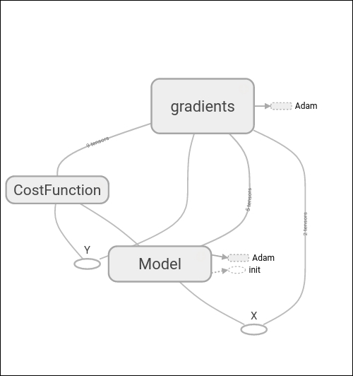
In the following diagram, we see the different actors of the whole setup: a model, the CostFunction, and the gradients. A really useful feature of TensorFlow is the ability to automatically differentiate between the Model and functions.
Here, we can find the definition of the variables represented in the preceding section: w, b, and the model linear equation.
X = tf.placeholder("float", name="X") # create symbolic variables
Y = tf.placeholder("float", name = "Y")

withtf.name_scope("Model"):
    w = tf.Variable(tf.random_normal([2], stddev=0.01), name="b0") # create a shared variable
    b = tf.Variable(tf.random_normal([2], stddev=0.01), name="b1") # create a shared variable
def model(X, w, b):
returntf.mul(X, w) + b # We just define the line as X*w + b0
y_model = model(X, w, b)
Loss function description and Optimizer loop
In this example, we will use the commonly employed mean squared error, but this time with a multivariable; so we apply reduce_mean to collect error values across the different dimensions:
withtf.name_scope("CostFunction"):
    cost = tf.reduce_mean(tf.pow(Y-y_model, 2)) # use sqr error for cost function
train_op = tf.train.AdamOptimizer(0.1).minimize(cost)
 for a in range (1,10):
    cost1=0.0
fori, j in zip(xvalues, yvalues):
sess.run(train_op, feed_dict={X: i, Y: j})
        cost1+=sess.run(cost, feed_dict={X: i, Y: i})/506.00
        #writer.add_summary(summary_str, i)
xvalues, yvalues = shuffle (xvalues, yvalues)
The stop condition will simply consist of training the parameters with all data samples for the number of epochs determined in the outer loop.
The following is the result:
1580.53295174
[ 2.25225258  1.30112672]
[ 0.80297691  0.22137061]
1512.3965525
[ 4.62365675  2.90244412]
[ 1.16225874  0.28009811]
1495.47174799
[ 6.52791834  4.29297304]
[ 0.824792270.17988272]
...
1684.6247849
[ 29.71323776  29.96078873]
[-0.68271929 -0.13493828]
1688.25864746
[ 29.78564262  30.09841156]
[-0.58272243 -0.08323665]
1684.27538102
[ 29.75390816  30.13044167]
[-0.59861398 -0.11895057]
From the results, we see that in the final stage of the training, the modeling lines settle on the following coefficients simultaneously:
price = 0.6 x Industry + 29.75
price = 0.1 x Age + 30.13
The following is the complete source code:
import matplotlib.pyplot as plt
import tensorflow as tf
import tensorflow.contrib.learn as skflow
from sklearn.utils import shuffle
import numpy as np
import pandas as pd
df = pd.read_csv("data/boston.csv", header=0)
printdf.describe()
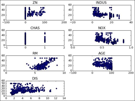
f, ax1 = plt.subplots()
plt.figure() # Create a new figure
y = df['MEDV']
for i in range (1,8):
number = 420 + i
ax1.locator_params(nbins=3)
ax1 = plt.subplot(number)
plt.title(list(df)[i])
ax1.scatter(df[df.columns[i]],y) #Plot a scatter draw of the datapoints
plt.tight_layout(pad=0.4, w_pad=0.5, h_pad=1.0)
X = tf.placeholder("float", name="X") # create symbolic variables
Y = tf.placeholder("float", name = "Y")
with tf.name_scope("Model"):
w = tf.Variable(tf.random_normal([2], stddev=0.01), name="b0") # create a shared variable
b = tf.Variable(tf.random_normal([2], stddev=0.01), name="b1") # create a shared variable
def model(X, w, b):
return tf.mul(X, w) + b # We just define the line as X*w + b0
y_model = model(X, w, b)
with tf.name_scope("CostFunction"):
cost = tf.reduce_mean(tf.pow(Y-y_model, 2)) # use sqr error for cost function
train_op = tf.train.AdamOptimizer(0.001).minimize(cost)
sess = tf.Session()
init = tf.initialize_all_variables()
tf.train.write_graph(sess.graph, '/home/bonnin/linear2','graph.pbtxt')
cost_op = tf.scalar_summary("loss", cost)
merged = tf.merge_all_summaries()
sess.run(init)
writer = tf.train.SummaryWriter('/home/bonnin/linear2', sess.graph)
xvalues = df[[df.columns[2], df.columns[4]]].values.astype(float)
yvalues = df[df.columns[12]].values.astype(float)
b0temp=b.eval(session=sess)
b1temp=w.eval(session=sess)
for a in range (1,10):
cost1=0.0
for i, j in zip(xvalues, yvalues):
sess.run(train_op, feed_dict={X: i, Y: j})
cost1+=sess.run(cost, feed_dict={X: i, Y: i})/506.00
#writer.add_summary(summary_str, i)
xvalues, yvalues = shuffle (xvalues, yvalues)
print (cost1)
b0temp=b.eval(session=sess)
b1temp=w.eval(session=sess)
print (b0temp)
print (b1temp)
#plt.plot (trX, b0temp + b1temp * trX )
In this chapter, we built our first complete model with a standard loss function using TensorFlow's training utilities. We also built a multivariate model to account for more than one dimension to calculate regression. Apart from that, we used TensorBoard to observe the variable's behavior during the training phase.
In the next chapter, we will begin working with non-linear models, through which we will get closer to the domain of neural networks, which is the main supported field of TensorFlow and the area where its utilities provide great value.