Chapter 5. Simple FeedForward Neural Networks
Neural Networks are really the area of Machine Learning where Tensorflow excels. Many types of architectures and algorithms can be implemented with it, along with the additional advantage of having a symbolic engine incorporated, which will really help in the training of more complex setups.
With this chapter, we are beginning to harness the power of high-performance primitives for solving increasingly complex problems with a high number of supported input variables.
In this chapter, we will cover the following topics:
- Preliminary concepts of neural networks
- Neural network projects on non-linear synthetic function regression
- Projects on predicting car fuel efficiency with nonlinear regression
- Learning to classify wines andmulticlass classification
To build a simple framework into the neural network components and architectures, we will give a simple and straightforward build of the original concepts which paved the way to the current,complexand variedNeural Network landscape.
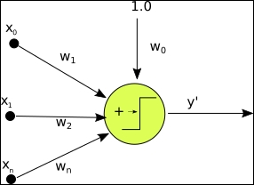
An artificial neuron is a mathematical function conceived as a model for a real biological neuron.
Its main features are that it receives one or more inputs (training data), and sums them to produce an output. Additionally, the sums are normally weighted (weight and bias), and the sum is passed to a nonlinear function (Activation function or transfer function).
Original example - the Perceptron
The Perceptron is one of the simplest ways of implementing an artificial neuron and it's an algorithm that dates back from the 1950s, first implemented in the 1960s.
It is basically an algorithm that learns a binary classification function, which maps a real function with a single binary one:
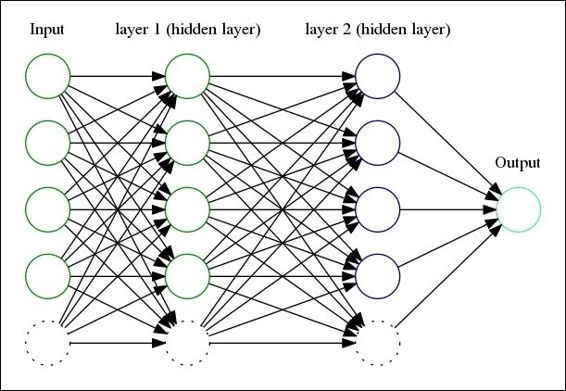
The following image shows a single layer perceptron
The simplified algorithm for the perceptron is:
- Initialize the weights with a random distribution (normally low values)
- Select an input vector and present it to the network,
- Compute the output y' of the network for the input vector specified and the values of the weights.
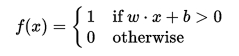
- The function for a perceptron is:
- If y' ≠ y modify all connections wi by adding the changes Δw =yxi
- Return to step 2.
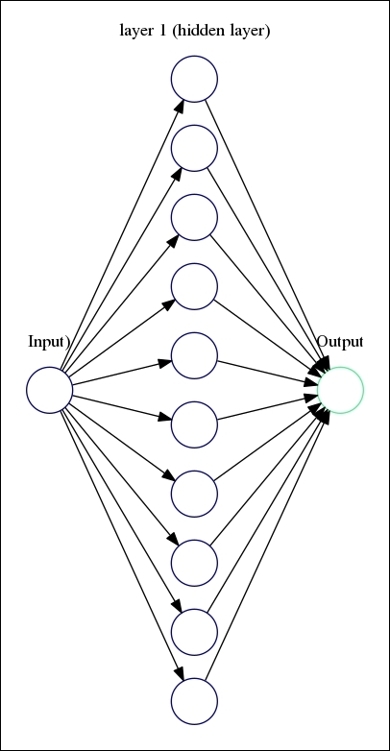
The single layer perceptron can be generalized to many layers connected to eachother, but there is an issue remaining;the representing function is a linear combination of the inputs, and the perceptron being just a kind of linear classifier,there is no possibility of correctly fitting a nonlinear function.
Neural Network activation functions
The learning properties of a Neural Network would not be so great with only the help of a univariate linear classifier. Even some mildly complex problemsin machine learning involve multiple nonlinear variables, so many variants were developed as replacements of the transfer functions of the perceptron.
In order to represent nonlinear models, a number of different nonlinear functions can be used in the activation function. This implies changes in the way the neurons will react to changes in the input variables. The most common activation functions used in practice are:
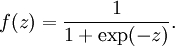
- Sigmoid : The canonical activation function, and has very good qualities for calculating probabilities in classification properties.
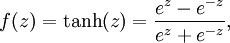
- Tanh: Very similar to the sigmoid, but its value range is [-1,1] instead of [0,1]
-
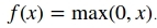
Relu
: This is called a rectified linear unit, and one of its main advantages is that it is not affected by the Vanishing Gradients problem, which generally exists on the first layers of a network to tend to values of 0, or a tiny epsilon:
Gradients and the back propagation algorithm
When we described the learning phase of the perceptron, we described a stage in which the weights were adjusted proportionally according to the "responsibility" of a weight in the final error.
In this complex network of neurons, the responsibility of the error will be distributed among all the functions applied to the data in the whole architecture.
So once we have calculated the total error, and we have the whole function applied to the original data, we must now try to adjust all variables in the equation to minimize it.
What we need to know to be able to minimize this error, as the Optimization field has studied, is the gradient of the loss function.
Given that the data goes through many weights and transfer functions, the resulting compound function's gradient will have to be solved by the chain rule.
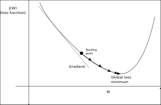
Minimizing loss function: Gradient descent
Lets have a look at the following graph to understand the loss function:
Neural networks problem choice - Classification vs Regression
Neural Networks can be used for regression problems and classification ones. The common architectural difference resides in the output layer: in order to be able to bring a real number base result, no standardization function, like sigmoid, should be applied.In this way, we won't be changing the outcomes of the variable to one of many possible class values, getting a continuum of possible outcomes.
Useful libraries and methods
In this chapter we will be using some new utilities from TensorFlow, and also from utility libraries, these would be the most important ones:
TensorFlow activation functions
Most commonly used functions for TensorFlow navigation:
- tf.sigmoid(x):The standard sigmoid function
- tf.tanh(x):Hyperbolic tangent
- tf.nn.relu(features):Relu transfer function
Other functions for TensorFlow navigation:
- tf.nn.elu(features): Computes exponential linear: exp(features) - 1 if < 0, features otherwise
- tf.nn.softsign(features): Computes softsign: features / (abs(features) + 1)
- tf.nn.bias_add(value, bias): Adds bias to value
TensorFlow loss optimization methods
TensorFlow Loss optimization methods are described in the following:
- tf.train.GradientDescentOptimizer(learning_rate, use_locking, name): This is the original Gradient descent method, with only the learning rate parameter
- tf.train.AdagradOptimizer(learning_rate, initial_accumulator_value, use_locking, name): This method adapts the learning rate, to the frequency of the parameters, improving the efficiency of the minimum search for sparse parameters
- tf.train.AdadeltaOptimizer (learning_rate, rho, epsilon, use_locking, name): This is a modified AdaGrad, which will restrict the accumulation of frequent parameters to a maximum window, so it takes in account a certain number of steps, and not the whole parameter history.
- tf.train.AdamOptimizertf.train.AdamOptimizer.__init__(learning_rate, beta1, beta2, epsilon, use_locking, name): This method adds a factor when calculating gradients, corresponding to the average of the past gradients, equivalent to a momentum factor. Thus the name Adam, from Adaptive Moment Estimation.
Sklearn preprocessing utilities
Lets have a look at the following Sklearn preprocessing utilities:
- preprocessing.StandardScaler(): Normalization of datasets is a common requirement for many machine learning estimators, so in order to make convergence more straightforward the dataset will have to be more like a standard normally distribution that is a Gaussian curve with zero mean and unit variance. In practice, we often ignore the shape of the distribution and just transform the data to center it by removing the mean value of each feature, then scale it by dividing non-constant features by their standard deviation. For this task, we use the StandardScaler, which implements the tasks previously mentioned. It also stores the transforms, in order to be able to reapply it to the testing set.
- StandardScaler .fit_transform(): Simply fit the data to the required form. The StandardScaler object will save the transform variables, so you will be able to get the denormalized data back.
- cross_validation.train_test_split: This method splits the dataset into train and test segments, we only need to provide the percentage of the dataset assigned to each stage.
First project - Non linear synthetic function regression
Artificial neural network examples normally include a great majority of classification problems, but in fact there are a great number of applications that could be expressed as regressions.
The network architectures used for regression don't differ in great measure from the ones used for classification problems: They can take multi-variable input and can use linear and nonlinear activation functions too.
In some cases, the only necessary case is just to remove the sigmoid-like function at the end of the layers to allow the full range of options to appear.
In this first example, we will model a simple, noisy quadratic function, and will try to regress it by means of a single hidden layer network and see how close we can be topredicting values taken from a test population.
Dataset description and loading
In this case, we will be using a generated dataset, which will be very similar to the one in Chapter 3, Linear Regression.
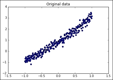
We will generate a quadratic function using the common Numpy methods, and then we will add random noise, which will help us to see how the linear regression can generalize.
The core sample creation routines are as follows:
import numpy as np
trainsamples = 200
testsamples = 60
dsX = np.linspace(-1, 1, trainsamples + testsamples).transpose()
dsY = 0.4* pow(dsX,2) +2 * dsX + np.random.randn(*dsX.shape) * 0.22 + 0.8
This dataset doesn't need preprocessing as it is being generated, and has good properties such asbeing centered and having a -1, 1 x sample distribution.
Modeling architecture - Loss Function description
The loss for this setup will simply be represented by the same as the mean squares error, with the line:
cost = tf.pow(py_x-Y, 2)/(2)
In this particular case we will be using the Gradient Descent cost optimizer, which we can invoke with the line:
train_op = tf.train.AdamOptimizer(0.5).minimize(cost)
Accuracy and Convergence test
predict_op = tf.argmax(py_x, 1)
cost1 += sess.run(cost, feed_dict={X: [[x1]], Y: y1}) / testsamples
Lets have a look at the example code shown in the following:
import tensorflow as tf
import numpy as np
from sklearn.utils import shuffle
%matplotlib inline
import matplotlib.pyplot as plt
trainsamples = 200
testsamples = 60
#Here we will represent the model, a simple imput, a hidden layer of sigmoid activation
def model(X, hidden_weights1, hidden_bias1, ow):
    hidden_layer =  tf.nn.sigmoid(tf.matmul(X, hidden_weights1)+ b)
    return tf.matmul(hidden_layer, ow)
dsX = np.linspace(-1, 1, trainsamples + testsamples).transpose()
dsY = 0.4* pow(dsX,2) +2 * dsX + np.random.randn(*dsX.shape) * 0.22 + 0.8
plt.figure() # Create a new figure
plt.title('Original data')
plt.scatter(dsX,dsY) #Plot a scatter draw of the datapoints
X = tf.placeholder("float")
Y = tf.placeholder("float")
# Create first hidden layer
hw1 = tf.Variable(tf.random_normal([1, 10], stddev=0.1))
# Create output connection
ow = tf.Variable(tf.random_normal([10, 1], stddev=0.0))
# Create bias
b = tf.Variable(tf.random_normal([10], stddev=0.1))
model_y = model(X, hw1, b, ow)
# Cost function
cost = tf.pow(model_y-Y, 2)/(2)
# construct an optimizer
train_op = tf.train.GradientDescentOptimizer(0.05).minimize(cost)
# Launch the graph in a session
with tf.Session() as sess:
    tf.initialize_all_variables().run() #Initialize all variables
    for i in range(1,100):
        dsX, dsY = shuffle (dsX.transpose(), dsY) #We randomize the samples to mplement a better training
        trainX, trainY =dsX[0:trainsamples], dsY[0:trainsamples]
        for x1,y1 in zip (trainX, trainY):
            sess.run(train_op, feed_dict={X: [[x1]], Y: y1})
        testX, testY = dsX[trainsamples:trainsamples + testsamples], dsY[0:trainsamples:trainsamples+testsamples]
        cost1=0.
        for x1,y1 in zip (testX, testY):
            cost1 += sess.run(cost, feed_dict={X: [[x1]], Y: y1}) / testsamples
        if (i%10 == 0):
            print "Average cost for epoch " + str (i) + ":" + str(cost1)
This is a copy of the different epoch results.Note that as this is a very simple function, even the first iteration has very good results:
Average cost for epoch 1:[[ 0.00753353]]
Average cost for epoch 2:[[ 0.00381996]]
Average cost for epoch 3:[[ 0.00134867]]
Average cost for epoch 4:[[ 0.01020064]]
Average cost for epoch 5:[[ 0.00240157]]
Average cost for epoch 6:[[ 0.01248318]]
Average cost for epoch 7:[[ 0.05143405]]
Average cost for epoch 8:[[ 0.00621457]]
Average cost for epoch 9:[[ 0.0007379]]
Second project - Modeling cars fuel efficiency with non linear regression
In this example, we will enter into an area where Neural Networks provide most of their added value; solving non linear problems. To begin this journey, we will be modeling a regression model for the fuel efficiency of several car models, based on several variables, which can be better represented by non linear functions.
Dataset description and loading
For this problem, we will be analyzing a very well-known, standard,well-formeddataset, which will allow us to analyze a multi-variable problem: guessing the mpg an automobile will have based on some related variables, discrete and continuous.
This could be considered a toy and somewhat dated example, but it will pave the way to more complex problems, and has the advantage of being already analyzed by numerous bibliographies.
Attribute Information
This dataset has the following data columns:
- mpg: continuous
- cylinders: multi-valued discrete
- displacement: continuous
- horsepower: continuous
- weight: continuous
- acceleration: continuous
- model year: multi-valued discrete
- origin: multi-valued discrete
- car name: string (won't be used)
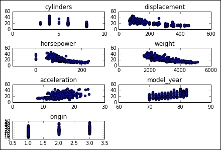
We won't be doing a detailed analysis of the data, but we can informally infer that all of the continuous variables have a correlation with increasing or decreasing the goal variable:
For this function, we will be using the previously-describedscaler objects, from sklearn:
- scaler =
preprocessing.StandardScaler()
- X_train =
scaler.fit_transform(X_train)
What we are about to build is a feedforward neural network, with a multivariate input, and a simple output:
score = metrics.mean_squared_error(regressor.predict(scaler.transform(X_test)), y_test)
print('MSE: {0:f}'.format(score))
Step #99, avg. train loss: 182.33624
Step #199, avg. train loss: 25.09151
Step #300, epoch #1, avg. train loss: 11.92343
Step #400, epoch #1, avg. train loss: 11.20414
Step #500, epoch #1, avg. train loss: 5.14056
Total Mean Squared Error: 15.0792258911
%matplotlib inline
import matplotlib.pyplot as plt
import pandas as pd

from sklearn import datasets, cross_validation, metrics
from sklearn import preprocessing
from tensorflow.contrib import skflow

# Read the original dataset
df = pd.read_csv("data/mpg.csv", header=0)
# Convert the displacement column as float
df['displacement']=df['displacement'].astype(float)
# We get data columns from the dataset
# First and last (mpg and car names) are ignored for X
X = df[df.columns[1:8]]
y = df['mpg']

plt.figure() # Create a new figure

for i in range (1,8):
    number = 420 + i
    ax1.locator_params(nbins=3)
    ax1 = plt.subplot(number)
    plt.title(list(df)[i])
    ax1.scatter(df[df.columns[i]],y) #Plot a scatter draw of the  datapoints
plt.tight_layout(pad=0.4, w_pad=0.5, h_pad=1.0)
# Split the datasets

X_train, X_test, y_train, y_test = cross_validation.train_test_split(X, y,
test_size=0.25)

# Scale the data for convergency optimization
scaler = preprocessing.StandardScaler()

# Set the transform parameters
X_train = scaler.fit_transform(X_train)

# Build a 2 layer fully connected DNN with 10 and 5 units respectively
regressor = skflow.TensorFlowDNNRegressor(hidden_units=[10, 5],
steps=500, learning_rate=0.051, batch_size=1)

# Fit the regressor
regressor.fit(X_train, y_train)

# Get some metrics based on the X and Y test data
score = metrics.mean_squared_error(regressor.predict(scaler.transform(X_test)), y_test)

print(" Total Mean Squared Error: " + str(score))
Third project - Learning to classify wines: Multiclass classification
In this section we will work with a more complex dataset, trying to classify wines based on theirplace of origin.
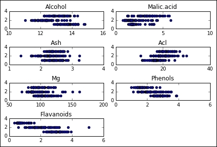
Dataset description and loading
This data contains the results of a chemical analysis of wines grown in the same region in Italy but derived from three different cultivars. The analysis determined the quantities of 13 constituents found in each of the three types of wines.
Data variables:
- Alcohol
- Malic acid
- Ash
- Alcalinity of ash
- Magnesium
- Total phenols
- Flavanoids
- Nonflavanoid phenols
- Proanthocyanins
- Color intensity
- Hue
- OD280/OD315 of diluted wines
- Proline
To read the dataset, we will simply use the provided CSV file and pandas:
df = pd.read_csv("./wine.csv", header=0)
As the values on the csv begin at 1, we will normalize the values resting the bias:
y = df['Wine'].values-1
For the results, we will have to represent the options as a one hot list of arrays:
Y = tf.one_hot(indices = y, depth=3, on_value = 1., off_value = 0., axis = 1 , name = "a").eval()
We will also shuffle the values beforehand:
X, Y = shuffle (X, Y)
scaler = preprocessing.StandardScaler()
X = scaler.fit_transform(X)
This particular model will consist of a single layer, fully-connected, neural network:
x = tf.placeholder(tf.float32, [None, 12])W = tf.Variable(tf.zeros([12, 3]))b = tf.Variable(tf.zeros([3]))y = tf.nn.softmax(tf.matmul(x, W) + b)
Loss function description
We will use the cross entropy function to measure loss:
y_ = tf.placeholder(tf.float32, [None, 3])
cross_entropy = tf.reduce_mean(-tf.reduce_sum(y_ * tf.log(y), reduction_indices=[1]))
Again the Gradient Descent method will be used to reduce the loss function:
train_step = tf.train.GradientDescentOptimizer(0.1).minimize(cross_entropy)
In the convergence test, we will cast every good regression to 1, and every false one to 0, and then get the mean of the values to measure the accuracy of the model:
correct_prediction = tf.equal(tf.argmax(y, 1), tf.argmax(y_, 1))
accuracy = tf.reduce_mean(tf.cast(correct_prediction, tf.float32))
print(accuracy.eval({x: Xt, y_: Yt}))
As we see, we have a variating accuracy as the epochs progress, but it is always superior to a 90% accuracy, with a 30% random base (if we'd generated a random number between 0 and 3 to guess the result).
0.973684
0.921053
0.921053
0.947368
0.921053
Lets have a look at the complete source code:
sess = tf.InteractiveSession()
import pandas as pd
# Import data
from tensorflow.examples.tlutorials.mnist import input_data
from sklearn.utils import shuffle
import tensorflow as tf

from sklearn import preprocessing

flags = tf.app.flags
FLAGS = flags.FLAGS

df = pd.read_csv("./wine.csv", header=0)
print (df.describe())
#df['displacement']=df['displacement'].astype(float)
X = df[df.columns[1:13]].values
y = df['Wine'].values-1
Y = tf.one_hot(indices = y, depth=3, on_value = 1., off_value = 0., axis = 1 , name = "a").eval()
X, Y = shuffle (X, Y)

scaler = preprocessing.StandardScaler()
X = scaler.fit_transform(X)

# Create the model
x = tf.placeholder(tf.float32, [None, 12])
W = tf.Variable(tf.zeros([12, 3]))
b = tf.Variable(tf.zeros([3]))
y = tf.nn.softmax(tf.matmul(x, W) + b)

# Define loss and optimizer
y_ = tf.placeholder(tf.float32, [None, 3])
cross_entropy = tf.reduce_mean(-tf.reduce_sum(y_ * tf.log(y), reduction_indices=[1]))
train_step = tf.train.GradientDescentOptimizer(0.1).minimize(cross_entropy)
# Train
tf.initialize_all_variables().run()
for i in range(100):
X,Y =shuffle (X, Y, random_state=1)

Xtr=X[0:140,:]
Ytr=Y[0:140,:]

Xt=X[140:178,:]
Yt=Y[140:178,:]
Xtr, Ytr = shuffle (Xtr, Ytr, random_state=0)
#batch_xs, batch_ys = mnist.train.next_batch(100)
batch_xs, batch_ys = Xtr , Ytr
train_step.run({x: batch_xs, y_: batch_ys})
cost = sess.run (cross_entropy, feed_dict={x: batch_xs, y_: batch_ys})
# Test trained model
correct_prediction = tf.equal(tf.argmax(y, 1), tf.argmax(y_, 1))
accuracy = tf.reduce_mean(tf.cast(correct_prediction, tf.float32))
print(accuracy.eval({x: Xt, y_: Yt}))
In this chapter, we have been starting the path toward implementing the real quid of TensorFlow capability: Neural Network models.
We have also seen the use of simple Neural Networks in both regression and classification tasks, with simple generated models, and experimental ones.
In the next chapter we will advance the knowledge of new architectures and ways of applying the Neural Network paradigm for other knowledge fields, such as computer vision, in the form of convolutional neural networks.