An example of decomposing language model probabilities word-by-word.
While the final goal of a statistical machine translation system is to create a model of the target sentence E given the source sentence F, P(E ∣ F), in this chapter we will take a step back, and attempt to create a of only the target sentence P(E). Basically, this model allows us to do two things that are of practical use.
Given a sentence E, this can tell us, does this look like an actual, natural sentence in the target language? If we can learn a model to tell us this, we can use it to assess the fluency of sentences generated by an automated system to improve its results. It could also be used to evaluate sentences generated by a human for purposes of grammar checking or error correction.
Language models can also be used to randomly generate text by sampling a sentence E′ from the target distribution: E′∼P(E).1 Randomly generating samples from a language model can be interesting in itself – we can see what the model “thinks” is a natural-looking sentences – but it will be more practically useful in the context of the neural translation models described in the following chapters.
In the following sections, we’ll cover a few methods used to calculate this probability P(E).
As mentioned above, we are interested in calculating the probability of a sentence E = e1T. Formally, this can be expressed as
P(E)=P(|E|=T, e1T),
the joint probability that the length of the sentence is (|E|=T), that the identity of the first word in the sentence is e1, the identity of the second word in the sentence is e2, up until the last word in the sentence being eT. Unfortunately, directly creating a model of this probability distribution is not straightforward,2 as the length of the sequence T is not determined in advance, and there are a large number of possible combinations of words.
An example of decomposing language model probabilities word-by-word.
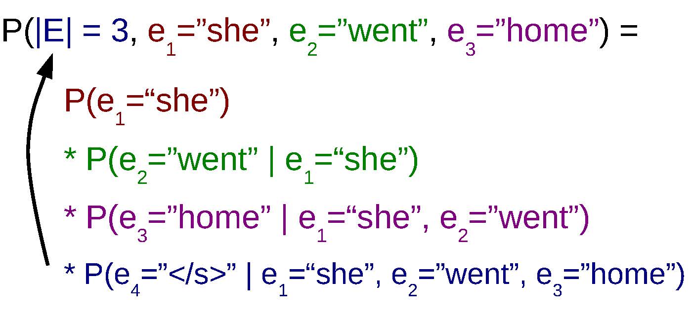
As a way to make things easier, it is common to re-write the probability of the full sentence as the product of single-word probabilities. This takes advantage of the fact that a joint probability – for example P(e1, e2, e3) – can be calculated by multiplying together conditional probabilities for each of its elements. In the example, this means that P(e1, e2, e3)=P(e1)P(e2 ∣ e1)P(e3 ∣ e1, e2).
shows an example of this incremental calculation of probabilities for the sentence “she went home”. Here, in addition to the actual words in the sentence, we have introduced an implicit sentence end (“$\sentend$”) symbol, which we will indicate when we have terminated the sentence. Stepping through the equation in order, this means we first calculate the probability of “she” coming at the beginning of the sentence, then the probability of “went” coming next in a sentence starting with “she”, the probability of “home” coming after the sentence prefix “she went”, and then finally the sentence end symbol “$\sentend$” after “she went home”. More generally, we can express this as the following equation:
$$P(E) = \prod_{t=1}^{T+1} P(e_t \mid e_1^{t-1})
\label{eq:ngramlm:prod}$$
where $e_{T+1}=\sentend$. So coming back to the sentence end symbol $\sentend$, the reason why we introduce this symbol is because it allows us to know when the sentence ends. In other words, by examining the position of the $\sentend$ symbol, we can determine the |E|=T term in our original LM joint probability in . In this example, when we have $\sentend$ as the 4th word in the sentence, we know we’re done and our final sentence length is 3.
Once we have the formulation in , the problem of language modeling now becomes a problem of calculating the next word given the previous words P(et ∣ e1t − 1). This is much more manageable than calculating the probability for the whole sentence, as we now have a fixed set of items that we are looking to calculate probabilities for. The next couple of sections will show a few ways to do so.
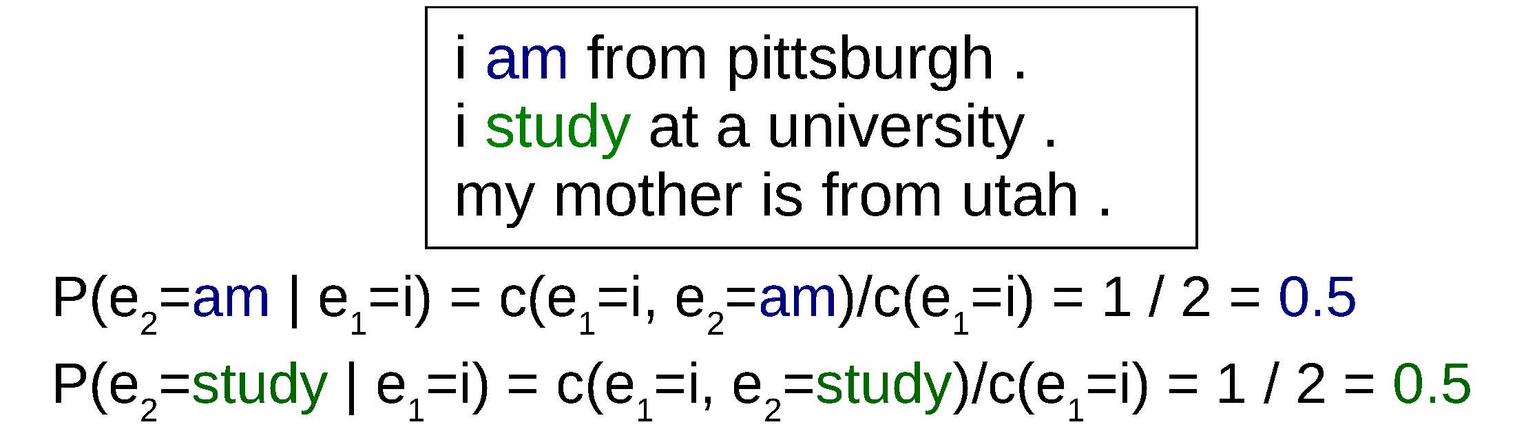
An example of calculating probabilities using maximum likelihood estimation.
The first way to calculate probabilities is simple: prepare a set of training data from which we can count word strings, count up the number of times we have seen a particular string of words, and divide it by the number of times we have seen the context. This simple method, can be expressed by the equation below, with an example shown in
$$P_{\text{ML}}(e_t \mid e_1^{t-1}) = \frac{c_{\text{prefix}}(e_1^t)}{c_{\text{prefix}}(e_1^{t-1})}.
\label{eq:ngramlm:wordbyword}$$
Here cprefix(⋅) is the count of the number of times this particular word string appeared at the beginning of a sentence in the training data. This approach is called (MLE, details later in this chapter), and is both simple and guaranteed to create a model that assigns a high probability to the sentences in training data.
However, let’s say we want to use this model to assign a probability to a new sentence that we’ve never seen before. For example, if we want to calculate the probability of the sentence “i am from utah .” based on the training data in the example. This sentence is extremely similar to the sentences we’ve seen before, but unfortunately because the string “i am from utah” has not been observed in our training data, cprefix(i, am, from, utah)=0, P(e4 = utah ∣ e1 = i, e2 = am, e3 = from) becomes zero, and thus the probability of the whole sentence as calculated by also becomes zero. In fact, this language model will assign a probability of zero to every sentence that it hasn’t seen before in the training corpus, which is not very useful, as the model loses ability to tell us whether a new sentence a system generates is natural or not, or generate new outputs.
To solve this problem, we take two measures. First, instead of calculating probabilities from the beginning of the sentence, we set a fixed window of previous words upon which we will base our probability calculations, approximating the true probability. If we limit our context to n − 1 previous words, this would amount to:
P(et ∣ e1t − 1)≈PML(et ∣ et − n + 1t − 1).
Models that make this assumption are called . Specifically, when models where n = 1 are called unigram models, n = 2 bigram models, n = 3 trigram models, and n ≥ 4 four-gram, five-gram, etc.
The parameters θ of n-gram models consist of probabilities of the next word given n − 1 previous words:
θet − n + 1t = P(et ∣ et − n + 1t − 1),
and in order to train an n-gram model, we have to learn these parameters from data. In the simplest form, these parameters can be calculated using maximum likelihood estimation as follows:
$$\theta_{e_{t-n+1}^{t}} = P_{\text{ML}}(e_t \mid e_{t-n+1}^{t-1}) = \frac{c(e_{t-n+1}^t)}{c(e_{t-n+1}^{t-1})},
\label{eq:ngramlm:mle}$$
where c(⋅) is the count of the word string anywhere in the corpus. Sometimes these equations will reference et − n + 1 where t − n + 1 < 0. In this case, we assume that $e_{t-n+1}=\sentbegin$ where $\sentbegin$ is a special sentence start symbol.
If we go back to our previous example and set n = 2, we can see that while the string “i am from utah .” has never appeared in the training corpus, “i am”, “am from”, “from utah”, “utah .”, and “. $\sentend$” are all somewhere in the training corpus, and thus we can patch together probabilities for them and calculate a non-zero probability for the whole sentence.
However, we still have a problem: what if we encounter a two-word string that has never appeared in the training corpus? In this case, we’ll still get a zero probability for that particular two-word string, resulting in our full sentence probability also becoming zero. n-gram models fix this problem by probabilities, combining the maximum likelihood estimates for various values of n. In the simple case of smoothing unigram and bigram probabilities, we can think of a model that combines together the probabilities as follows:
P(et ∣ et − 1)=(1 − α)PML(et ∣ et − 1)+αPML(et),
where α is a variable specifying how much probability mass we hold out for the unigram distribution. As long as we set α > 0, regardless of the context all the words in our vocabulary will be assigned some probability. This method is called , and is one of the standard ways to make probabilistic models more robust to low-frequency phenomena.
If we want to use even more context – n = 3, n = 4, n = 5, or more – we can recursively define our interpolated probabilities as follows:
P(et ∣ et − m + 1t − 1)=(1 − αm)PML(et ∣ et − m + 1t − 1)+αmP(et ∣ et − m + 2t − 1).
The first term on the right side of the equation is the maximum likelihood estimate for the model of order m, and the second term is the interpolated probability for all orders up to m − 1.
There are also more sophisticated methods for smoothing, which are beyond the scope of this section, but summarized very nicely in .
Instead of having a fixed α, we condition the interpolation coefficient on the context: αet − m + 1t − 1. This allows the model to give more weight to higher order n-grams when there are a sufficient number of training examples for the parameters to be estimated accurately and fall back to lower-order n-grams when there are fewer training examples. These context-dependent smoothing coefficients can be chosen using heuristics or learned from data .
In , we interpolated together two probability distributions over the full vocabulary V. In the alternative formulation of , the lower-order distribution only is used to calculate probabilities for words that were given a probability of zero in the higher-order distribution. Back-off is more expressive but also more complicated than interpolation, and the two have been reported to give similar results .
It is also possible to use a different distribution than PML. This can be done by subtracting a constant value from the counts before calculating probabilities, a method called . It is also possible to modify the counts of lower-order distributions to reflect the fact that they are used mainly as a fall-back for when the higher-order distributions lack sufficient coverage.
Currently, (MKN; ), is generally considered one of the standard and effective methods for smoothing n-gram language models. MKN uses context-dependent smoothing coefficients, discounting, and modification of lower-order distributions to ensure accurate probability estimates.
Once we have a language model, we will want to test whether it is working properly. The way we test language models is, like many other machine learning models, by preparing three sets of data:
is used to train the parameters θ of the model.
is used to make choices between alternate models, or to tune the of the model. Hyper-parameters in the model above could include the maximum length of n in the n-gram model or the type of smoothing method.
is used to measure our final accuracy and report results.
For language models, we basically want to know whether the model is an accurate model of language, and there are a number of ways we can define this. The most straight-forward way of defining accuracy is the of the model with respect to the development or test data. The likelihood of the parameters θ with respect to this data is equal to the probability that the model assigns to the data. For example, if we have a test dataset ℰtest, this is:
P(ℰtest; θ).
We often assume that this data consists of several independent sentences or documents E, giving us
P(ℰtest; θ)=∏E ∈ ℰtestP(E; θ).
Another measure that is commonly used is
logP(ℰtest; θ)=∑E ∈ ℰtestlogP(E; θ).
The log likelihood is used for a couple reasons. The first is because the probability of any particular sentence according to the language model can be a very small number, and the product of these small numbers can become a very small number that will cause numerical precision problems on standard computing hardware. The second is because sometimes it is more convenient mathematically to deal in log space. For example, when taking the derivative in gradient-based methods to optimize parameters (used in the next section), it is more convenient to deal with the sum in than the product in .
It is also common to divide the log likelihood by the number of words in the corpus
length(ℰtest)=∑E ∈ ℰtest|E|.
This makes it easier to compare and contrast results across corpora of different lengths.
The final common measure of language model accuracy is , which is defined as the exponent of the average negative log likelihood per word
ppl(ℰtest; θ)=e−(logP(ℰtest; θ))/length(ℰtest).
An intuitive explanation of the perplexity is “how confused is the model about its decision?” More accurately, it expresses the value “if we randomly picked words from the probability distribution calculated by the language model at each time step, on average how many words would it have to pick to get the correct one?” One reason why it is common to see perplexities in research papers is because the numbers calculated by perplexity are bigger, making the differences in models more easily perceptible by the human eye.3
Finally, one important point to keep in mind is that some of the words in the test set ℰtest will not appear even once in the training set ℰtrain. These words are called , and need to be handeled in some way. Common ways to do this in language models include:
Sometimes we can assume that there will be no new words in the test set. For example, if we are calculating a language model over ASCII characters, it is reasonable to assume that all characters have been observed in the training set. Similarly, in some speech recognition systems, it is common to simply assign a probability of zero to words that don’t appear in the training data, which means that these words will not be able to be recognized.
As mentioned in , we can interpolate between distributions of higher and lower order. In the case of unknown words, we can think of this as a distribution of order “0”, and define the 1-gram probability as the interpolation between the unigram distribution and unknown word distribution
$$P(e_t) = (1 - \alpha_1) P_{\text{ML}}(e_t) + \alpha_1 P_{\text{\text{unk}}}(e_t).
\label{eq:ngramlm:unkinterpolation}$$
Here, $P_{\text{\text{unk}}}$ needs to be a distribution that assigns a probability to all words Vall, not just ones in our vocabulary V derived from the training corpus. This could be done by, for example, training a language model over characters that “spells out” unknown words in the case they don’t exist in in our vocabulary. Alternatively, as a simpler approximation that is nonetheless fairer than ignoring unknown words, we can guess the total number of words |Vall| in the language where we are modeling, where |Vall|>|V|, and define $P_{\text{\text{unk}}}$ as a uniform distribution over this vocabulary: $P_{\text{\text{unk}}}(e_t) = 1/|V_{\text{all}}|$.
As a final method to handle unknown words we can remove some of the words in ℰtrain from our vocabulary, and replace them with a special $\sentunk$ symbol representing unknown words. One common way to do so is to remove , or words that only appear once in the training corpus. By doing this, we explicitly predict in which contexts we will be seeing an unknown word, instead of implicitly predicting it through interpolation like mentioned above. Even if we predict the $\sentunk$ symbol, we will still need to estimate the probability of the actual word, so any time we predict $\sentunk$ at position i, we further multiply in the probability of Punk(et).
To read in more detail about n-gram language models, gives a very nice introduction and comprehensive summary about a number of methods to overcome various shortcomings of vanilla n-grams like the ones mentioned above.
There are also a number of extensions to n-gram models that may be nice for the interested reader.
Language models are an integral part of many commercial applications, and in these applications it is common to build language models using massive amounts of data harvested from the web for other sources. To handle this data, there is research on efficient data structures , distributed parameter servers , and lossy compression algorithms .
In many situations, we want to build a language model for specific speaker or domain. Adaptation techniques make it possible to create large general-purpose models, then adapt these models to more closely match the target use case .
As mentioned above, n-gram models limit their context to n − 1, but in reality there are dependencies in language that can reach much farther back into the sentence, or even span across whole documents. The recurrent neural network language models that we will introduce in are one way to handle this problem, but there are also non-neural approaches such as cache language models , topic models , and skip-gram models .
There are also models that take into account the syntax of the target sentence. For example, it is possible to condition probabilities not on words that occur directly next to each other in the sentence, but those that are “close” syntactically .
The exercise that we will be doing in class will be constructing an n-gram LM with linear interpolation between various levels of n-grams. We will write code to:
Read in and save the training and testing corpora.
Learn the parameters on the training corpus by counting up the number of times each n-gram has been seen, and calculating maximum likelihood estimates according to .
Calculate the probabilities of the test corpus using linearly interpolation according to or .
To handle unknown words, you can use the uniform distribution method described in , assuming that there are 10,000,000 words in the English vocabulary. As a sanity check, it may be better to report the number of unknown words, and which portions of the per-word log-likelihood were incurred by the main model, and which portion was incurred by the unknown word probability logPunk.
In order to do so, you will first need data, and to make it easier to start out you can use some pre-processed data from the German-English translation task of the IWSLT evaluation campaign4 here: http://phontron.com/data/iwslt-en-de-preprocessed.tar.gz.
Potential improvements to the model include reading and implementing a better smoothing method, implementing a better method for handling unknown words, or implementing one of the more advanced methods in .