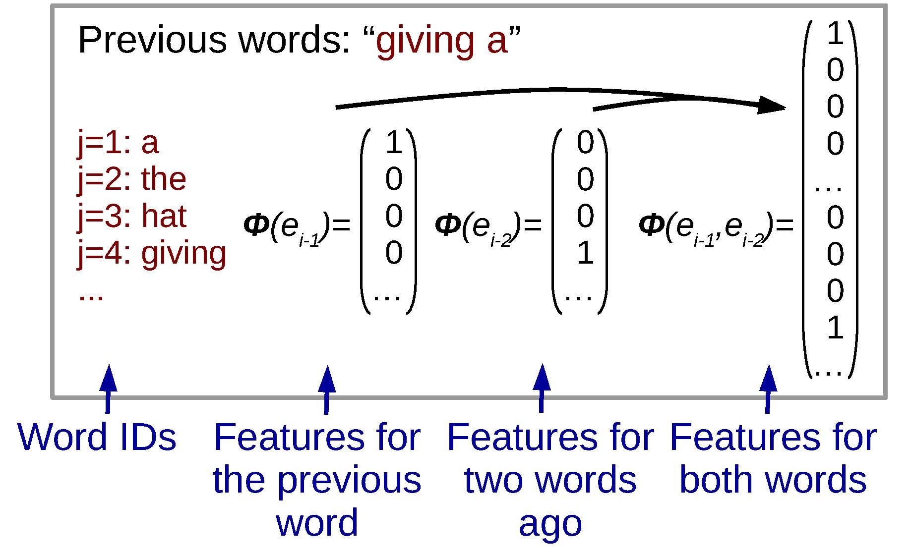
An example of feature values for a particular context.
This chapter will discuss another set of language models: , which take a very different approach than the count-based n-grams described above.1
Like n-gram language models, log-linear language models still calculate the probability of a particular word et given a particular context et − n + 1t − 1. However, their method for doing so is quite different from count-based language models, based on the following procedure.
Calculating features: Log-linear language models revolve around the concept of . In short, features are basically, “something about the context that will be useful in predicting the next word”. More formally, we define a feature function ϕ(et − n + 1t − 1) that takes a context as input, and outputs a real-valued x ∈ ℝN that describe the context using N different features.2
An example of feature values for a particular context.
For example, from our bi-gram models from the previous chapter, we know that “the identity of the previous word” is something that is useful in predicting the next word. If we want to express the identity of the previous word as a real-valued vector, we can assume that each word in our vocabulary V is associated with a word ID j, where 1 ≤ j ≤ |V|. Then, we define our feature function ϕ(et − n + 1t) to return a feature vector x = ℝ|V|, where if et − 1 = j, then the jth element is equal to one and the remaining elements in the vector are equal to zero. This type of vector is often called a , an example of which is shown in (a). For later user, we will also define a function onehot(i) which returns a vector where only the ith element is one and the rest are zero (assume the length of the vector is the appropriate length given the context).
Of course, we are not limited to only considering one previous word. We could also calculate one-hot vectors for both et − 1 and et − 2, then concatenate them together, which would allow us to create a model that considers the values of the two previous words. In fact, there are many other types of feature functions that we can think of (more in ), and the ability to flexibly define these features is one of the advantages of log-linear language models over standard n-gram models.
Calculating scores: Once we have our feature vector, we now want to use these features to predict probabilities over our output vocabulary V. In order to do so, we calculate a score vector s ∈ ℝ|V| that corresponds to the likelihood of each word: words with higher scores in the vector will also have higher probabilities. We do so using the model parameters θ, which specifically come in two varieties: a b ∈ ℝ|V|, which tells us how likely each word in the vocabulary is overall, and a W = ℝ|V|×N which describes the relationship between feature values and scores. Thus, the final equation for calculating our scores for a particular context is:
s = Wx + b.
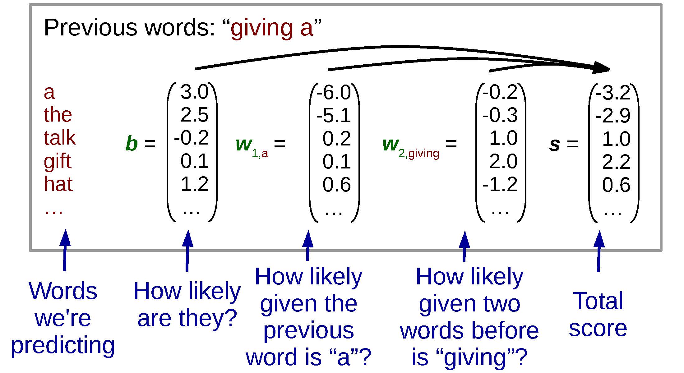
An example of the weights for a log linear model in a certain context.
One thing to note here is that in the special case of one-hot vectors or other sparse vectors where most of the elements are zero. Because of this we can also think about in a different way that is numerically equivalent, but can make computation more efficient. Specifically, instead of multiplying the large feature vector by the large weight matrix, we can add together the columns of the weight matrix for all active (non-zero) features as follows:
s = ∑{j : xj ≠ 0}W⋅, jxj + b,
where W⋅, j is the jth column of W. This allows us to think of calculating scores as “look up the vector for the features active for this instance, and add them together”, instead of writing them as matrix math. An example calculation in this paradigm where we have two feature functions (one for the directly preceding word, and one for the word before that) is shown in .
Calculating probabilities: It should be noted here that scores s are arbitrary real numbers, not probabilities: they can be negative or greater than one, and there is no restriction that they add to one. Because of this, we run these scores through a function that performs the following transformation:
$$p_j = \frac{\text{exp}( s_j )}{\sum_{\tilde{j}} \text{exp}( s_{\tilde{j}} )}.
\label{eq:lllm:softmaxsum}$$
By taking the exponent and dividing by the sum of the values over the entire vocabulary, these scores can be turned into probabilities that are between 0 and 1 and sum to 1.
This function is called the function, and often expressed in vector form as follows:
p = softmax(s).
Through applying this to the scores calculated in the previous section, we now have a way to go from features to language model probabilities.
Now, the only remaining missing link is how to acquire the parameters θ, consisting of the weight matrix W and bias b. Basically, the way we do so is by attempting to find parameters that fit the training corpus well.
To do so, we use standard machine learning methods for optimizing parameters. First, we define a ℓ(⋅) – a function expressing how poorly we’re doing on the training data. In most cases, we assume that this loss is equal to the :
ℓ(ℰtrain, θ)= − logP(ℰtrain ∣ θ)= − ∑E ∈ ℰtrainlogP(E ∣ θ).
We assume we can also define the loss on a per-word level:
ℓ(et − n + 1t, θ)=logP(et ∣ et − n + 1t − 1).
Next, we optimize the parameters to reduce this loss. While there are many methods for doing so, in recent years one of the go-to methods is (SGD). SGD is an iterative process where we randomly pick a single word et (or mini-batch, discussed in ) and take a step to improve the likelihood with respect to et. In order to do so, we first calculate the derivative of the loss with respect to each of the features in the full feature set θ:
$$\frac{d\ell(e_{t-n+1}^t,\bm{\theta})}{d\bm{\theta}}.$$
We can then use this information to take a step in the direction that will reduce the loss according to the objective function
$$\bm{\theta} \leftarrow \bm{\theta} - \eta \frac{d\ell(e_{t-n+1}^t,\bm{\theta})}{d\bm{\theta}},$$
where η is our , specifying the amount with which we update the parameters every time we perform an update. By doing so, we can find parameters for our model that reduce the loss, or increase the likelihood, on the training data.
This vanilla variety of SGD is quite simple and still a very competitive method for optimization in large-scale systems. However, there are also a few things to consider to ensure that training remains stable:
SGD requires also requires us to carefully choose η: if η is too big, training can become unstable and diverge, and if η is too small, training may become incredibly slow or fall into bad local optima. One way to handle this problem is : starting with a higher learning rate, then gradually reducing the learning rate near the end of training. Other more sophisticated methods are listed below.
It is common to use a held-out development set, measure our log-likelihood on this set, and save the model that has achieved the best log-likelihood on this held-out set. This is useful in case the model starts to over-fit to the training set, losing its generalization capability, we can re-wind to this saved model. As another method to prevent over-fitting and smooth convergence of training, it is common to measure log likelihood on a held-out development set, and when the log likelihood stops improving or starts getting worse, reduce the learning rate.
One of the features of SGD is that it processes training data one at a time. This is nice because it is simple and can be efficient, but it also causes problems if there is some bias in the order in which we see the data. For example, if our data is a corpus of news text where news articles come first, then sports, then entertainment, there is a chance that near the end of training our model will see hundreds or thousands of entertainment examples in a row, resulting in the parameters moving to a space that favors these more recently seen training examples. To prevent this problem, it is common (and highly recommended) to randomly shuffle the order with which the training data is presented to the learning algorithm on every pass through the data.
There are also a number of other update rules that have been proposed to improve gradient descent and make it more stable or efficient. Some representative methods are listed below:
Instead of taking a single step in the direction of the current gradient, SGD with momentum keeps an exponentially decaying average of past gradients. This reduces the propensity of simple SGD to “jitter” around, making optimization move more smoothly across the parameter space.
AdaGrad focuses on the fact that some parameters are updated much more frequently than others. For example, in the model above, columns of the weight matrix W corresponding to infrequent context words will only be updated a few times for every pass through the corpus, while the bias b will be updated on every training example. Based on this, AdaGrad dynamically adjusts the training rate η for each parameter individually, with frequently updated (and presumably more stable) parameters such as b getting smaller updates, and infrequently updated parameters such as W getting larger updates.
Adam is another method that computes learning rates for each parameter. It does so by keeping track of exponentially decaying averages of the mean and variance of past gradients, incorporating ideas similar to both momentum and AdaGrad. Adam is now one of the more popular methods for optimization, as it greatly speeds up convergence on a wide variety of datasets, facilitating fast experimental cycles. However, it is also known to be prone to over-fitting, and thus, if high performance is paramount, it should be used with some caution and compared to more standard SGD methods.
provides a good overview of these various methods with equations and notes a few other concerns when performing stochastic optimization.
Now, the final piece in the puzzle is the calculation of derivatives of the loss function with respect to the parameters. To do so, first we step through the full loss function in one pass as below:
$$\begin{aligned}
\bm{x} & = \bm{\phi}(e_{t-m+1}^{t-1}) \\
\bm{s} & = \sum_{\{j:x_j != 0\}} W_{\cdot,j} x_j + \bm{b} \\
\bm{p} & = \text{softmax}( \bm{s} ) \\
\ell & = - \log \bm{p}_{e_t}.\end{aligned}$$
And thus, using the chain rule to calculate
$$\begin{aligned}
\frac{d\ell(e_{t-n+1}^t, W, \bm{b})}{d\bm{b}} & = \frac{d\ell}{d\bm{p}} \frac{d\bm{p}}{d\bm{s}} \frac{d\bm{s}}{d\bm{b}} \\
\frac{d\ell(e_{t-n+1}^t, W, \bm{b})}{dW_{\cdot,j}} & = \frac{d\ell}{d\bm{p}} \frac{d\bm{p}}{d\bm{s}} \frac{d\bm{s}}{dW_{\cdot,j}}\end{aligned}$$
we find that the derivative of the loss function for the bias and each column of the weight matrix is:
$$\begin{aligned}
\frac{d\ell(e_{t-n+1}^t, W, \bm{b})}{d\bm{b}} & = \bm{p} - \text{onehot}(e_t) \\
\frac{d\ell(e_{t-n+1}^t, W, \bm{b})}{dW_{\cdot,j}} & = x_j (\bm{p} - \text{onehot}(e_t))\end{aligned}$$
Confirming these equations is left as a (highly recommended) exercise to the reader. Hint: when performing this derivation, it is easier to work with the log probability logp than working with p directly.
One reason why log-linear models are nice is because they allow us to flexibly design features that we think might be useful for predicting the next word. For example, these could include:
As shown in the example above, we can use the identity of et − 1 or the identity of et − 2.
Context words can be grouped into classes of similar words (using a method such as Brown clustering ), and instead of looking up a one-hot vector with a separate entry for every word, we could look up a one-hot vector with an entry for each class . Thus, words from the same class could share statistical strength, allowing models to generalize better.
Maybe we want a feature that fires every time the previous word ends with “...ing” or other common suffixes. This would allow us to learn more generalized patterns about words that tend to follow progressive verbs, etc.
Instead of just using the past n words, we could use all previous words in the sentence. This would amount to calculating the one-hot vectors for every word in the previous sentence, and then instead of concatenating them simply summing them together. This would lose all information about what word is in what position, but could capture information about what words tend to co-occur within a sentence or document.
It is also possible to combine together multiple features (for example et − 1 is a particular word and et − 2 is another particular word). This is one way to create a more expressive feature set, but also has a downside of greatly increasing the size of the feature space. We discuss these features in more detail in .
The language model in this section was basically a featurized version of an n-gram language model. There are quite a few other varieties of linear featurized models including:
These models, instead of predicting words one-by-one, predict the probability over the whole sentence then normalize . This can be conducive to introducing certain features, such as a probability distribution over lengths of sentences, or features such as “whether this sentence contains a verb”.
In the case that we want to use a language model to determine whether the output of a system is good or not, sometimes it is useful to train directly on this system output, and try to re-rank the outputs to achieve higher accuracy . Even if we don’t have real negative examples, it can be possible to “hallucinate” negative examples that are still useful for training .
In the exercise for this chapter, we will construct a log-linear language model and evaluate its performance. I highly suggest that you try to use the NumPy library to hold and perform calculations over feature vectors, as this will make things much easier. If you have never used NumPy before, you can take a look at this tutorial to get started: https://docs.scipy.org/doc/numpy-dev/user/quickstart.html.
Writing the program will entail:
Writing a function to read in the training and test corpora, and converting the words into numerical IDs.
Writing the feature function ϕ(et − n + 1t − 1), which takes in a string and returns which features are active (for example, as a baseline these can be features with the identity of the previous two words).
Writing code to calculate the loss function.
Writing code to calculate gradients and perform stochastic gradient descent updates.
Writing (or re-using from the previous exercise) code to evaluate the language models.
Similarly to the n-gram language models, we will measure the per-word log likelihood and perplexity on our text corpus, and compare it to n-gram language models. Handling unknown words will similarly require that you use the uniform distribution with 10,000,000 words in the English vocabulary.
Potential improvements to the model include designing better feature functions, adjusting the learning rate and measuring the results, and researching and implementing other types of optimizers such as AdaGrad or Adam.
It should be noted that the cited papers call these . This is because models in this chapter can be motivated in two ways: log-linear models that calculate un-normalized log-probability scores for each function and normalize them to probabilities, and maximum-entropy models that spread their probability mass as evenly as possible given the constraint that they must model the training data. While the maximum-entropy interpretation is quite interesting theoretically and interested readers can reference to learn more, the explanation as log-linear models is simpler conceptually, and thus we will use this description in this chapter.↩
Alternative formulations that define feature functions that also take the current word as input ϕ(et − n + 1t) are also possible, but in this book, to simplify the transition into neural language models described in , we consider features over only the context.↩