5 Neural Networks and Feed-forward Language Model

In this chapter, we describe language models based on , a way to learn more sophisticated functions to improve the accuracy of our probability estimates with less feature engineering.

Potential and Problems with Combination Features

An example of the effect that combining multiple words can have on the probability of the next word.

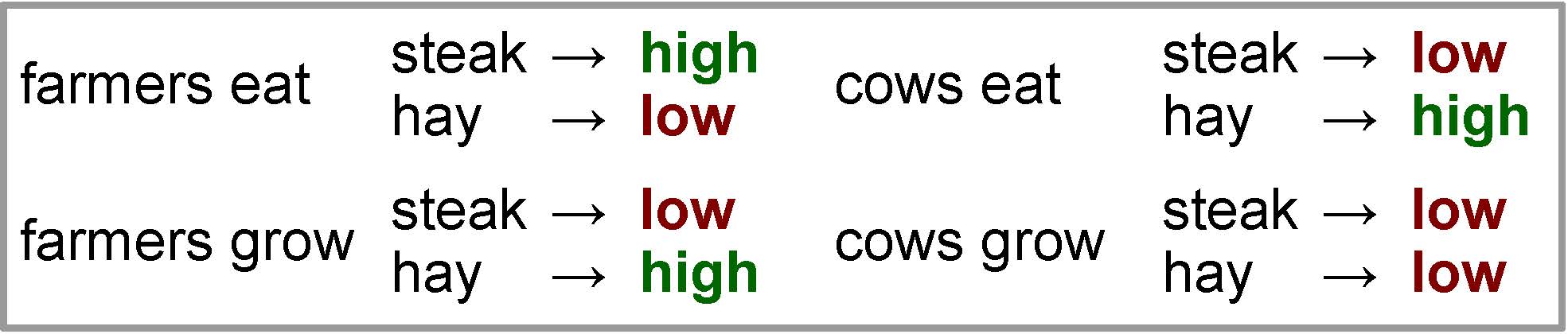
Before moving into the technical detail of neural networks, first let’s take a look at a motivating example in . From the example, we can see e_t − 2 = “farmers” is compatible with e_t = “hay” (in the context “farmers grow hay”), and e_t − 1 = “eat” is also compatible (in the context “cows eat hay”). If we are using a log-linear model with one set of features dependent on e_t − 1, and another set of features dependent on e_t − 2, neither set of features can rule out the unnatural phrase “farmers eat hay.”

One way we can fix this problem is by creating another set of features where we learn one vector for each pair of words e_t − 2, e_t − 1. If this is the case, our vector for the context e_t − 2 = “farmers”, e_t − 1 = “eat” could assign a low score to “hay”, resolving this problem. However, adding these combination features has one major disadvantage: it greatly expands the parameters: instead of O(|V|²) parameters for each pair e_i − 1, e_i, we need O(|V|³) parameters for each triplet e_i − 2, e_i − 1, e_i. These numbers greatly increase the amount of memory used by the model, and if there are not enough training examples, the parameters may not be learned properly.

Because of both the importance of and difficulty in learning using these combination features, a number of methods have been proposed to handle these features, such as and . Specifically in this section, we will cover neural networks, which are both flexible and relatively easy to train on large data, desiderata for sequence-to-sequence models.

A Brief Overview of Neural Networks

To understand neural networks in more detail, let’s take a very simple example of a function that we cannot learn with a simple linear classifier like the ones we used in the last chapter: a function that takes an input x ∈ { − 1, 1}² and outputs y = 1 if both x₁ and x₂ are equal and y = −1 otherwise. This function is shown in .

A function that cannot be solved by a linear transformation.

A first attempt at solving this function might define a linear model (like the log-linear models from the previous chapter) that solves this problem using the following form:
y = Wx + b.
However, this class of functions is not powerful enough to represent the function at hand.

Thus, we turn to a slightly more complicated class of functions taking the following form:
$$\begin{aligned} \bm{h} & = \text{step}(W_{xh} \bm{x} + \bm{b}_h) \nonumber \\ y & = \bm{w}_{hy} \bm{h} + b_y. \label{eq:nnlm:stepmlp}\end{aligned}$$
Computation is split into two stages: calculation of the , which takes in input x and outputs a vector of hidden variables h, and calculation of the , which takes in h and calculates the final result y. Both layers consist of an ¹ using weights W and biases b, followed by a step(⋅) function, which calculates the following:
$$\text{step}(x) = \begin{cases} 1 & \mbox{if } x > 0, \\ -1 & \mbox{otherwise}. \\ \end{cases}$$
This function is one example of a class of neural networks called (MLPs). In general, MLPs consist one or more hidden layers that consist of an affine transform followed by a non-linear function (such as the step function used here), culminating in an output layer that calculates some variety of output.

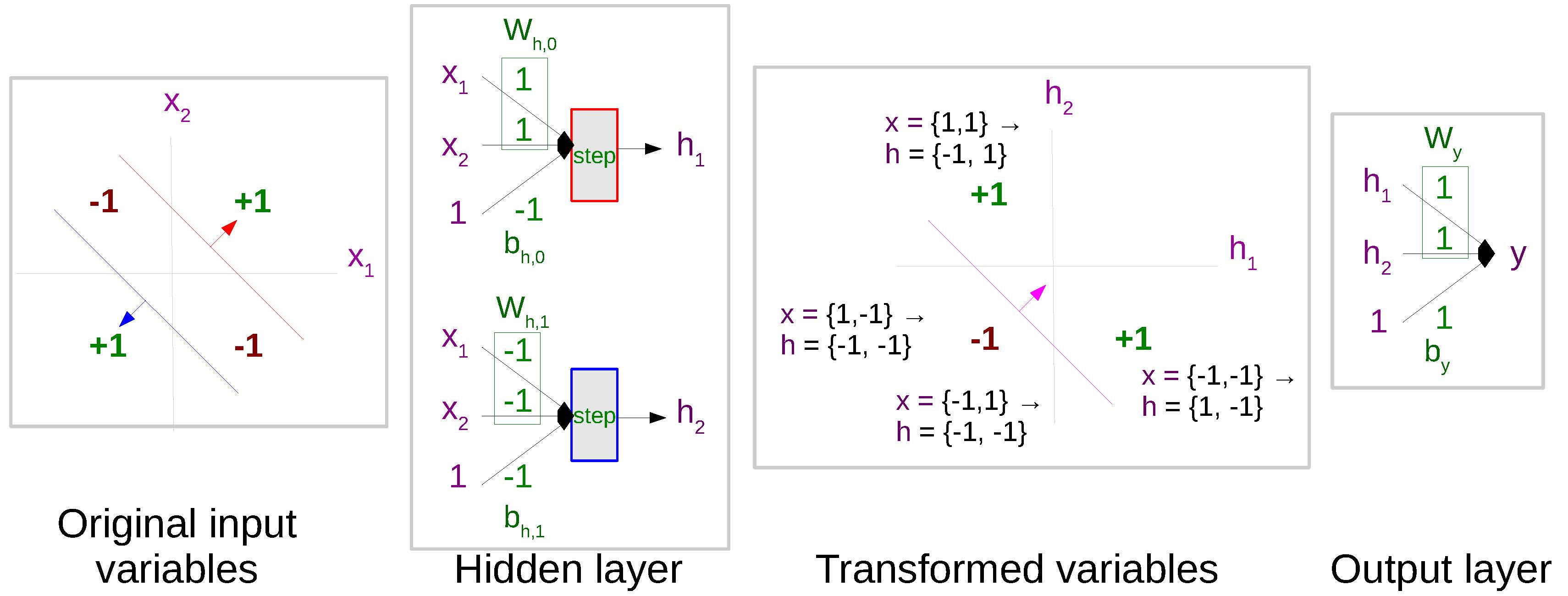
A simple neural network that represents the nonlinear function of .

demonstrates why this type of network does a better job of representing the non-linear function of . In short, we can see that the first hidden layer transforms the input x into a hidden vector h in a different space that is more conducive for modeling our final function. Specifically in this case, we can see that h is now in a space where we can define a linear function (using w_y and b_y) that correctly calculates the desired output y.

As mentioned above, MLPs are one specific variety of neural network. More generally, neural networks can be thought of as a chain of functions (such as the affine transforms and step functions used above, but also including many, many others) that takes some input and calculates some desired output. The power of neural networks lies in the fact that chaining together a variety of simpler functions makes it possible to represent more complicated functions in an easily trainable, parameter-efficient way. In fact, the simple single-layer MLP described above is a , which means that it can approximate any function to arbitrary accuracy if its hidden vector h is large enough.

We will see more about training in and give some more examples of how these can be more parameter efficient in the discussion of neural network language models in .

Training Neural Networks

Now that we have a model in , we would like to train its parameters W_mh, b_h, w_hy, and b_y. To do so, remembering our gradient-based training methods from the last chapter, we need to define the loss function ℓ(⋅), calculate the derivative of the loss with respect to the parameters, then take a step in the direction that will reduce the loss. For our loss function, let’s use the , a commonly used loss function for regression problems which measures the difference between the calculated value y and correct value y^* as follows
ℓ(y^*, y)=(y^* − y)².

Next, we need to calculate derivatives. Here, we run into one problem: the step(⋅) function is not very derivative friendly, with its derivative being:
$$\frac{d\text{step}(x)}{dx} = \begin{cases} \text{undefined} & \mbox{if } x = 0, \\ 0 & \mbox{otherwise}. \\ \end{cases}$$
Because of this, it is more common to use other non-linear functions, such as the hyperbolic tangent (tanh) function. The tanh function, as shown in , looks very much like a softened version of the step function that has a continuous gradient everywhere, making it more conducive to training with gradient-based methods. There are a number of other alternatives as well, the most popular of which being the rectified linear unit (RelU)
$$\text{RelU}(x) = \begin{cases} x & \mbox{if } x > 0, \\ 0 & \mbox{otherwise}. \\ \end{cases}$$
shown in the left of . In short, RelUs solve the problem that the tanh function gets “saturated” and has very small gradients when the absolute value of input x is very large (x is a large negative or positive number). Empirical results have often shown it to be an effective alternative to tanh, including for the language modeling task described in this chapter .

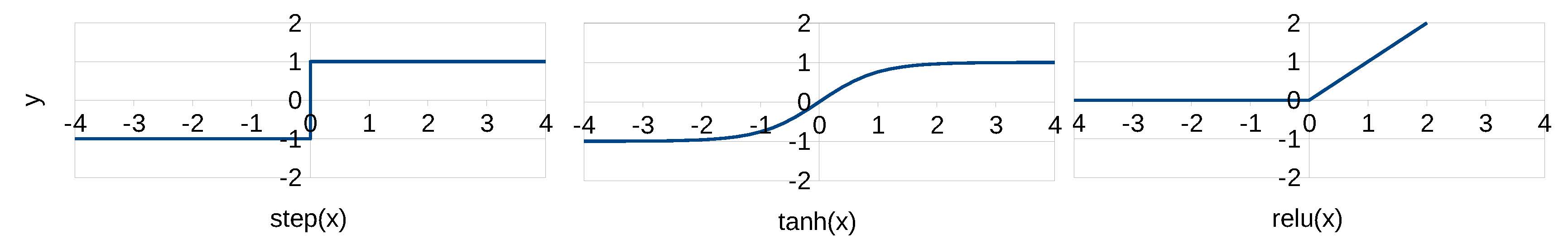
Types of non-linearities.

So let’s say we swap in a tanh non-linearity instead of the step function to our network, we can now proceed to calculate derivatives like we did in . First, we perform the full calculation of the loss function:
$$\begin{aligned} \bm{h}' & = W_{xh}\bm{x} + \bm{b}_h \nonumber \\ \bm{h} & = \tanh(\bm{h}') \nonumber \\ y & = \bm{w}_{hy}\bm{h} + b_y \nonumber \\ \ell & = (y^{*} - y)^2. \label{eq:nnlm:forward}\end{aligned}$$
Then, again using the chain rule, we calculate the derivatives of each set of parameters:
$$\begin{aligned} \frac{d\ell}{db_y} & = \frac{d\ell}{dy} \frac{dy}{db_y} \nonumber \\ \frac{d\ell}{d\bm{w}_{hy}} & = \frac{d\ell}{dy} \frac{dy}{d\bm{w}_{hy}} \nonumber \\ \frac{d\ell}{d\bm{b}_h} & = \frac{d\ell}{dy} \frac{dy}{d\bm{h}} \frac{d\bm{h}}{d\bm{h}'} \frac{d\bm{h}'}{d\bm{b}_h} \nonumber \\ \frac{d\ell}{dW_{xh}} & = \frac{d\ell}{dy} \frac{dy}{d\bm{h}} \frac{d\bm{h}}{d\bm{h}'} \frac{d\bm{h}'}{dW_{xh}}. \label{eq:nnlm:backward}\end{aligned}$$

We could go through all of the derivations above by hand and precisely calculate the gradients of all parameters in the model. Interested readers are free to do so, but even for a simple model like the one above, it is quite a lot of work and error prone. For more complicated models, like the ones introduced in the following chapters, this is even more the case.

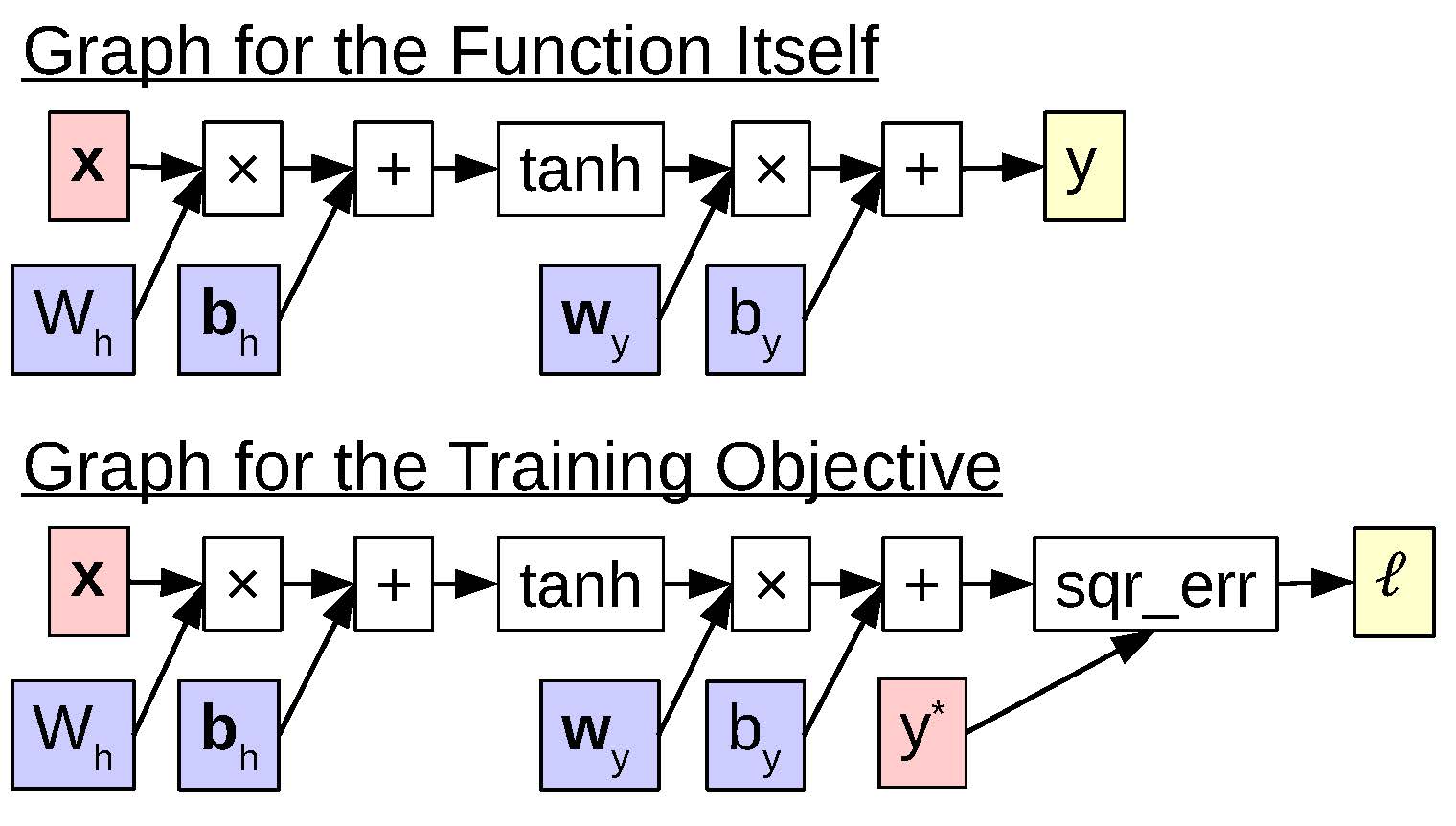
Computation graphs for the function itself, and the loss function.

Fortunately, when we actually implement neural networks on a computer, there is a very useful tool that saves us a large portion of this pain: (autodiff) . To understand automatic differentiation, it is useful to think of our computation in as a data structure called a , two examples of which are shown in . In these graphs, each node represents either an input to the network or the result of one computational operation, such as a multiplication, addition, tanh, or squared error. The first graph in the figure calculates the function of interest itself and would be used when we want to make predictions using our model, and the second graph calculates the loss function and would be used in training.

Automatic differentiation is a two-step dynamic programming algorithm that operates over the second graph and performs:

• , which traverses the nodes in the graph in topological order, calculating the actual result of the computation as in .

• , which traverses the nodes in reverse topological order, calculating the gradients as in .

The nice thing about this formulation is that while the overall function calculated by the graph can be relatively complicated, as long as it can be created by combining multiple simple nodes for which we are able to calculate the function f(x) and derivative f′(x), we are able to use automatic differentiation to calculate its derivatives using this dynamic program without doing the derivation by hand.

Thus, to implement a general purpose training algorithm for neural networks, it is necessary to implement these two dynamic programs, as well as the atomic forward function and backward derivative computations for each type of node that we would need to use. While this is not trivial in itself, there are now a plethora of toolkits that either perform general-purpose auto-differentiation , or auto-differentiation specifically tailored for machine learning and neural networks . These implement the data structures, nodes, back-propogation, and parameter optimization algorithms needed to train neural networks in an efficient and reliable way, allowing practitioners to get started with designing their models. In the following sections, we will take this approach, taking a look at how to create our models of interest in a toolkit called DyNet,² which has a programming interface that makes it relatively easy to implement the sequence-to-sequence models covered here.³

An Example Implementation

python import dynet as dy import random # Parameters of the model and training HIDDEN_SIZE = 20 NUM_EPOCHS = 20 # Define the model and SGD optimizer model = dy.Model() W_xh_p = model.add_parameters((HIDDEN_SIZE, 2)) b_h_p = model.add_parameters(HIDDEN_SIZE) W_hy_p = model.add_parameters((1, HIDDEN_SIZE)) b_y_p = model.add_parameters(1) trainer = dy.SimpleSGDTrainer(model) # Define the training data, consisting of (x,y) tuples data = [([1,1],1), ([-1,1],-1), ([1,-1],-1), ([-1,-1],1)] # Define the function we would like to calculate def calc_function(x): dy.renew_cg() w_xh = dy.parameter(w_xh_p) b_h = dy.parameter(b_h_p) W_hy = dy.parameter(W_hy_p) b_y = dy.parameter(b_y_p) x_val = dy.inputVector(x) h_val = dy.tanh(w_xh * x_val + b_h) y_val = W_hy * h_val + b_y return y_val # Perform training for epoch in range(NUM_EPOCHS): epoch_loss = 0 random.shuffle(data) for x, ystar in data: y = calc_function(x) loss = dy.squared_distance(y, dy.scalarInput(ystar)) epoch_loss += loss.value() loss.backward() trainer.update() print(“Epoch # Print results of prediction for x, ystar in data: y = calc_function(x) print(”

shows an example of implementing the above neural network in DyNet, which we’ll step through line-by-line. Lines 1-2 import the necessary libraries. Lines 4-5 specify parameters of the models: the size of the hidden vector h and the number of epochs (passes through the data) for which we’ll perform training. Line 7 initializes a DyNet model, which will store all the parameters we are attempting to learn. Lines 8-11 initialize parameters W_xh, b_h, w_hy, and b_y to be the appropriate size so that dimensions in the equations for match. Line 12 initializes a “trainer”, which will update the parameters in the model according to an update strategy (here we use simple stochastic gradient descent, but trainers for AdaGrad, Adam, and other strategies also exist). Line 14 creates the training data for the function in .

Lines 16-25 define a function that takes input x and creates a computation graph to calculate . First, line 17 creates a new computation graph to hold the computation for this particular training example. Lines 18-21 take the parameters (stored in the model) and adds them to the computation graph as DyNet variables for this particular training example. Line 22 takes a Python list representing the current input and puts it into the computation graph as a DyNet variable. Line 23 calculates the hidden vector h, Line 24 calculates the value y, and Line 25 returns it.

Lines 27-36 perform training for NUM_EPOCHS passes over the data (one pass through the training data is usually called an “epoch”). Line 28 creates a variable to keep track of the loss for this epoch for later reporting. Line 29 shuffles the data, as recommended in . Lines 30-35 perform stochastic gradient descent, looping over each of the training examples. Line 31 creates a computation for the function itself, and Line 32 adds computation for the loss function. Line 33 runs the forward calculation to calculate the loss and adds it to the loss for this epoch. Line 34 runs back propagation, and Line 35 updates the model parameters. At the end of the epoch, we print the loss for the epoch in Line 36 to make sure that the loss is going down and our model is converging.

Finally, at the end of training in Lines 38-40, we print the output results. In an actual scenario, this would be done on a separate set of test data.

Neural-network Language Models

Now that we have the basics down, it is time to apply neural networks to language modeling . A feed-forward neural network language model is very much like the log-linear language model that we mentioned in the previous section, simply with the addition of one or more non-linear layers before the output.

First, let’s recall the tri-gram log-linear language model. In this case, assume we have two sets of features expressing the identity of e_t − 1 (represented as W⁽¹⁾) and e_t − 2 (as W⁽²⁾), the equation for the log-linear model looks like this:
$$\begin{aligned} \bm{s} & = W^{(1)}_{\cdot,e_{t-1}} + W^{(2)}_{\cdot,e_{t-2}} + \bm{b} \nonumber \\ \bm{p} & = \text{softmax}(\bm{s}),\end{aligned}$$
where we add the appropriate columns from the weight matricies to the bias to get the score, then take the softmax to turn it into a probability.

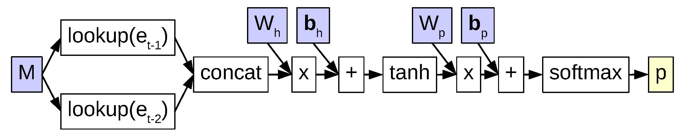
A computation graph for a tri-gram feed-forward neural language model.

Compared to this, a tri-gram neural network model with a single layer is structured as shown in and described in equations below:
$$\begin{aligned} \bm{m} & = \text{concat}(M_{\cdot,e_{t-2}},M_{\cdot,e_{t-1}}) \nonumber \\ \bm{h} & = \text{tanh}(W_{mh} \bm{m} + \bm{b}_h) \nonumber \\ \bm{s} & = W_{hs} \bm{h} + \bm{b}_s \nonumber \\ \bm{p} & = \text{softmax}(\bm{s}) \label{eq:nnlm:nnlm}\end{aligned}$$

In the first line, we obtain a vector m representing the context e_{i − n + 1}^i − 1 (in the particular case above, we are handling a tri-gram model so n = 3). Here, M is a matrix with |V| columns, and L_m rows, where each column corresponds to an L_m-length vector representing a single word in the vocabulary. This vector is called a or a , which is a vector of real numbers corresponding to particular words in the vocabulary.⁴ The interesting thing about expressing words as vectors of real numbers is that each element of the vector could reflect a different aspect of the word. For example, there may be an element in the vector determining whether a particular word under consideration could be a noun, or another element in the vector expressing whether the word is an animal, or another element that expresses whether the word is countable or not.⁵ shows an example of how to define parameters that allow you to look up a vector in DyNet.

python # Define the lookup parameters at model definition time # VOCAB_SIZE is the number of words in the vocabulary # EMBEDDINGS_SIZE is the length of the word embedding vector M_p = model.add_lookup_parameters((VOCAB_SIZE, EMBEDDING_SIZE)) # Load the parameters into the computation graph M = dy.lookup(M_p) # And look up the vector for word i m = M[i]

The vector m then results from the concatenation of the word vectors for all of the words in the context, so |m|=L_m * (n − 1). Once we have this m, we run the vectors through a hidden layer to obtain vector h. By doing so, the model can learn combination features that reflect information regarding multiple words in the context. This allows the model to be expressive enough to represent the more difficult cases in . For example, given a context is “cows eat”, and some elements of the vector M_⋅, cows identify the word as a “large farm animal” (e.g. “cow”, “horse”, “goat”), while some elements of M_⋅, eat corresponds to “eat” and all of its relatives (“consume”, “chew”, “ingest”), then we could potentially learn a unit in the hidden layer h that is active when we are in a context that represents “things farm animals eat”.

Next, we calculate the score vector for each word: s ∈ ℝ^|V|. This is done by performing an affine transform of the hidden vector h with a weight matrix W_hs ∈ ℝ^|V|×|h| and adding a bias vector b_s ∈ ℝ^|V|. Finally, we get a probability estimate p by running the calculated scores through a softmax function, like we did in the log-linear language models. For training, if we know e_t we can also calculate the loss function as follows, similarly to the log-linear model:
ℓ = −log(p_et).
DyNet has a convenience function that, given a score vector s, will calculate the negative log likelihood loss:

python loss = dy.pickneglogsoftmax(s, e_t)

The reasons why the neural network formulation is nice becomes apparent when we compare this to n-gram language models in :

Better generalization of contexts:

n-gram language models treat each word as its own discrete entity. By using input embeddings M, it is possible to group together similar words so they behave similarly in the prediction of the next word. In order to do the same thing, n-gram models would have to explicitly learn word classes and using these classes effectively is not a trivial problem .

More generalizable combination of words into contexts:

In an n-gram language model, we would have to remember parameters for all combinations of {cow, horse, goat}×{consume, chew, ingest} to represent the context “things farm animals eat”. This would be quadratic in the number of words in the class, and thus learning these parameters is difficult in the face of limited training data. Neural networks handle this problem by learning nodes in the hidden layer that can represent this quadratic combination in a feature-efficient way.

Ability to skip previous words:

n-gram models generally fall back sequentially from longer contexts (e.g. “the two previous words e_t − 2^t − 1”) to shorter contexts (e.g. “the previous words e_t − 1”), but this doesn’t allow them to “skip” a word and only reference for example, “the word two words ago e_t − 2”. Log-linear models and neural networks can handle this skipping naturally.

Further Reading

In addition to the methods described above, there are a number of extensions to neural-network language models that are worth discussing.

Softmax approximations:

One problem with the training of log-linear or neural network language models is that at every training example, they have to calculate the large score vector s, then run a softmax over it to get probabilities. As the vocabulary size |V| grows larger, this can become quite time-consuming. As a result, there are a number of ways to reduce training time. One example are methods that sample a subset of the vocabulary V′∈V where |V′| ≪ V, then calculate the scores and approximate the loss over this smaller subset. Examples of these include methods that simply try to get the true word e_t to have a higher score (by some margin) than others in the subsampled set and more probabilistically motivated methods, such as or (NCE; ). Interestingly, for other objective functions such as linear regression and special variety of softmax called the , it is possible to calculate the objective function in ways that do not scale linearly with the vocabulary size .

Other softmax structures:

Another interesting trick to improve training speed is to create a softmax that is structured so that its loss functions can be computed efficiently. One way to do so is the class-based softmax , which assigns each word e_t to a class c_t, then divides computation into two steps: predicting the probability of class c_t given the context, then predicting the probability of the word e_t given the class and the current context P(e_t ∣ c_t, e_{t − n + 1}^t − 1)P(c_t ∣ e_{t − n + 1}^t − 1). The advantage of this method is that we only need to calculate scores for the correct class c_t out of |C| classes, then the correct word e_t out of the vocabulary for class c_t, which is size |V_ct|. Thus, our computational complexity becomes O(|C|+|V_ct|) instead of O(|V|). The hierarchical softmax takes this a step further by predicting words along a binary-branching tree, which results in a computational complexity of O(log₂|V|).

Other models to learn word representations:

As mentioned in , we learn word embeddings M as a by-product of training our language models. One very nice feature of word representations is that language models can be trained purely on raw text, but the resulting representations can capture semantic or syntactic features of the words, and thus can be used to effectively improve down-stream tasks that don’t have a lot of annotated data, such as part-of-speech tagging or parsing .⁶ Because of their usefulness, there have been an extremely large number of approaches proposed to learn different varieties of word embeddings,⁷ from early work based on distributional similarity and dimensionality reduction to more recent models based on predictive models similar to language models , with the general current thinking being that predictive models are the more effective and flexible of the two .The most well-known methods are the continuous-bag-of-words and skip-gram models implemented in the software word2vec,⁸ which define simple objectives for predicting words using the immediately surrounding context or vice-versa. word2vec uses a sampling-based approach and parallelization to easily scale up to large datasets, which is perhaps the primary reason for its popularity. One thing to note is that these methods are not language models in themselves, as they do not calculate a probability of the sentence P(E), but many of the parameter estimation techniques can be shared.

Exercise

In the exercise for this chapter, we will use DyNet to construct a feed-forward language model and evaluate its performance.

Writing the program will entail:

• Writing a function to read in the data and (turn it into numerical IDs).

• Writing a function to calculate the loss function by looking up word embeddings, then running them through a multi-layer perceptron, then predicting the result.

• Writing code to perform training using this function.

• Writing evaluation code that measures the perplexity on a held-out data set.

Language modeling accuracy should be measured in the same way as previous exercises and compared with the previous models.

Potential improvements to the model include tuning the various parameters of the model. How big should h be? Should we add additional hidden layers? What optimizer with what learning rate should we use? What happens if we implement one of the more efficient versions of the softmax explained in ?