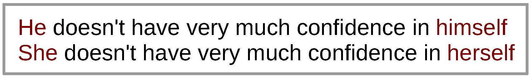
An example of long-distance dependencies in language.
The neural-network models presented in the previous chapter were essentially more powerful and generalizable versions of n-gram models. In this section, we talk about language models based on recurrent neural networks (RNNs), which have the additional ability to capture long-distance dependencies in language.
An example of long-distance dependencies in language.
Before speaking about RNNs in general, it’s a good idea to think about the various reasons a model with a limited history would not be sufficient to properly model all phenomena in language.
One example of a long-range is shown in . In this example, there is a strong constraint that the starting “he” or “her” and the final “himself” or “herself” must match in gender. Similarly, based on the subject of the sentence, the conjugation of the verb will change. These sorts of dependencies exist regardless of the number of intervening words, and models with a finite history ei − n + 1i − 1, like the one mentioned in the previous chapter, will never be able to appropriately capture this. These dependencies are frequent in English but even more prevalent in languages such as Russian, which has a large number of forms for each word, which must match in case and gender with other words in the sentence.1
Another example where long-term dependencies exist is in . In a nutshell, selectional preferences are basically common sense knowledge of “what will do what to what”. For example, “I ate salad with a fork” is perfectly sensible with “a fork” being a tool, and “I ate salad with my friend” also makes sense, with “my friend” being a companion. On the other hand, “I ate salad with a backpack” doesn’t make much sense because a backpack is neither a tool for eating nor a companion. These selectional preference violations lead to nonsensical sentences and can also span across an arbitrary length due to the fact that subjects, verbs, and objects can be separated by a great distance.
Finally, there are also dependencies regarding the or of the sentence or document. For example, it would be strange if a document that was discussing a technical subject suddenly started going on about sports – a violation of topic consistency. It would also be unnatural for a scientific paper to suddenly use informal or profane language – a lack of consistency in register.
These and other examples describe why we need to model long-distance dependencies to create workable applications.
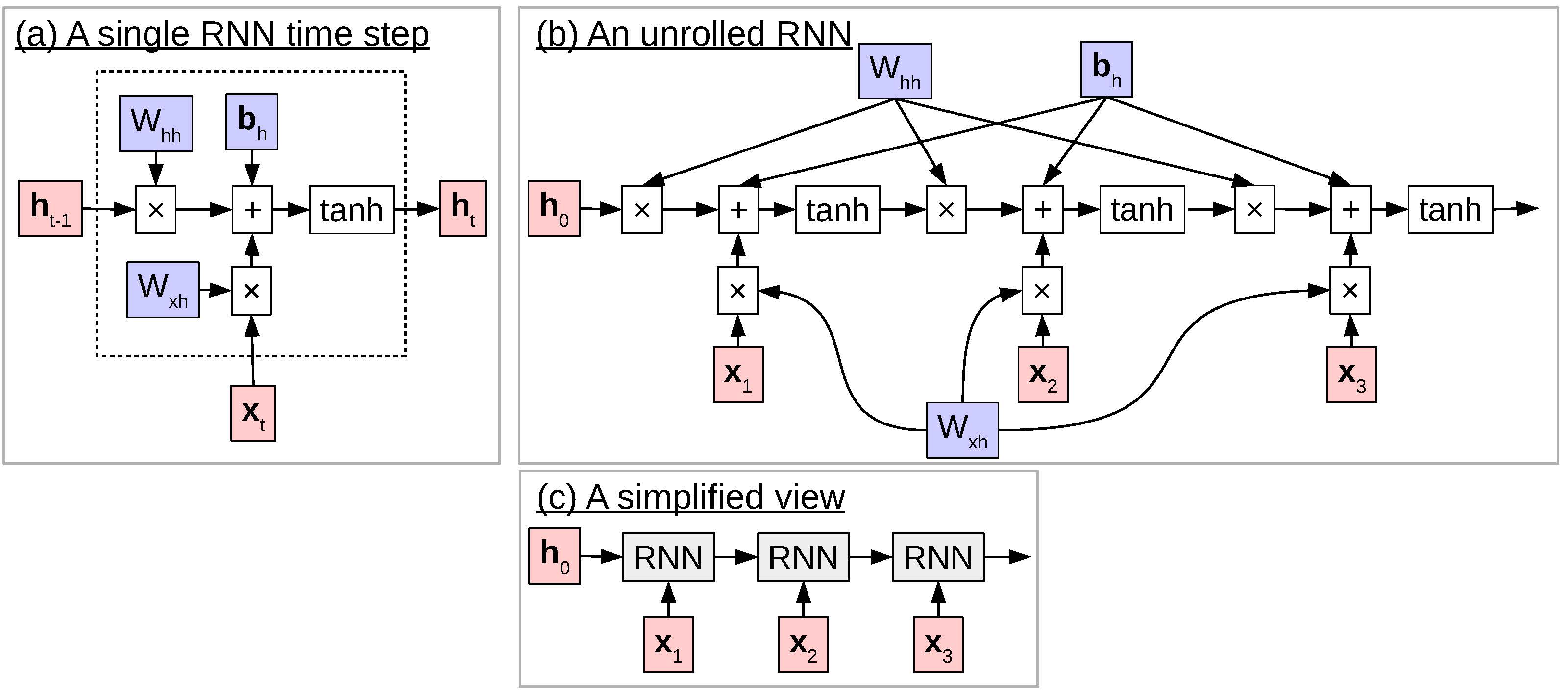
Examples of computation graphs for neural networks. (a) shows a single time step. (b) is the unrolled network. (c) is a simplified version of the unrolled network, where gray boxes indicate a function that is parameterized (in this case by Wxh, Whh, and bh).
(RNNs; ) are a variety of neural network that makes it possible to model these long-distance dependencies. The idea is simply to add a connection that references the previous hidden state ht − 1 when calculating hidden state h, written in equations as:
$$\bm{h}_t = \begin{cases}
\text{tanh}(W_{xh} \bm{x}_t + W_{hh} \bm{h}_{t-1} + \bm{b}_h) & t \ge 1, \\
\bm{0} & \mbox{otherwise}. \\
\end{cases}
\label{eq:rnnlm:rnn}$$
As we can see, for time steps t ≥ 1, the only difference from the hidden layer in a standard neural network is the addition of the connection Whhht − 1 from the hidden state at time step t − 1 connecting to that at time step t. As this is a recursive equation that uses ht − 1 from the previous time step. This single time step of a recurrent neural network is shown visually in the computation graph shown in (a).
When performing this visual display of RNNs, it is also common to “unroll” the neural network in time as shown in (b), which makes it possible to explicitly see the information flow between multiple time steps. From unrolling the network, we can see that we are still dealing with a standard computation graph in the same form as our feed-forward networks, on which we can still do forward computation and backward propagation, making it possible to learn our parameters. It also makes clear that the recurrent network has to start somewhere with an initial hidden state h0. This initial state is often set to be a vector full of zeros, treated as a parameter hinit and learned, or initialized according to some other information (more on this in ).
Finally, for simplicity, it is common to abbreviate the whole recurrent neural network step with a single block “RNN” as shown in . In this example, the boxes corresponding to RNN function applications are gray, to show that they are internally parameterized with Wxh, Whh, and bh. We will use this convention in the future to represent parameterized functions.
RNNs make it possible to model long distance dependencies because they have the ability to pass information between timesteps. For example, if some of the nodes in ht − 1 encode the information that “the subject of the sentence is male”, it is possible to pass on this information to ht, which can in turn pass it on to ht + 1 and on to the end of the sentence. This ability to pass information across an arbitrary number of consecutive time steps is the strength of recurrent neural networks, and allows them to handle the long-distance dependencies described in .
Once we have the basics of RNNs, applying them to language modeling is (largely) straight-forward . We simply take the feed-forward language model of and enhance it with a recurrent connection as follows:
$$\begin{aligned}
\bm{m}_t & = M_{\cdot,e_{t-1}} \nonumber \\
\bm{h}_t & = \begin{cases}
\text{tanh}(W_{mh} \bm{m}_t + W_{hh} \bm{h}_{t-1} + \bm{b}_h) & t \ge 1, \\
\bm{0} & \mbox{otherwise}. \\
\end{cases} \nonumber \\
\bm{p}_t & = \text{softmax}(W_{hs} \bm{h}_t + b_s).
\label{eq:rnnlm:rnnlm}\end{aligned}$$
One thing that should be noted is that compared to the feed-forward language model, we are only feeding in the previous word instead of the two previous words. The reason for this is because (if things go well) we can expect that information about et − 2 and all previous words are already included in ht − 1, making it unnecessary to feed in this information directly.
Also, for simplicity of notation, it is common to abbreviate the equation for ht with a function RNN(⋅), following the simplified view of drawing RNNs in (c):
$$\begin{aligned}
\bm{m}_t & = M_{\cdot,e_{t-1}} \nonumber \\
\bm{h}_t & = \text{RNN}(\bm{m}_t, \bm{h}_{t-1}) \nonumber \\
\bm{p}_t & = \text{softmax}(W_{hs} \bm{h}_t + b_s).
\label{eq:rnnlm:rnnlmabbrv}\end{aligned}$$

An example of the vanishing gradient problem.
However, while the RNNs in the previous section are conceptually simple, they also have problems: the problem and the closely related cousin, the problem.
A conceptual example of the vanishing gradient problem is shown in . In this example, we have a recurrent neural network that makes a prediction after several times steps, a model that could be used to classify documents or perform any kind of prediction over a sequence of text. After it makes its prediction, it gets a loss that it is expected to back-propagate over all time steps in the neural network. However, at each time step, when we run the back propagation algorithm, the gradient gets smaller and smaller, and by the time we get back to the beginning of the sentence, we have a gradient so small that it effectively has no ability to have a significant effect on the parameters that need to be updated. The reason why this effect happens is because unless $\frac{d\bm{h}_{t-1}}{d\bm{h}_t}$ is exactly one, it will tend to either diminish or amplify the gradient $\frac{d\ell}{d\bm{h}_t}$, and when this diminishment or amplification is done repeatedly, it will have an exponential effect on the gradient of the loss.2
One method to solve this problem, in the case of diminishing gradients, is the use of a neural network architecture that is specifically designed to ensure that the derivative of the recurrent function is exactly one. A neural network architecture designed for this very purpose, which has enjoyed quite a bit of success and popularity in a wide variety of sequential processing tasks, is the (LSTM; ) neural network architecture. The most fundamental idea behind the LSTM is that in addition to the standard hidden state h used by most neural networks, it also has a c, for which the gradient $\frac{d\bm{c}_{t}}{d\bm{c}_{t-1}}$ is exactly one. Because this gradient is exactly one, information stored in the memory cell does not suffer from vanishing gradients, and thus LSTMs can capture long-distance dependencies more effectively than standard recurrent neural networks.

A single time step of long short-term memory (LSTM). The information flow between the h and cell c is modulated using parameterized input and output gates.
So how do LSTMs do this? To understand this, let’s take a look at the LSTM architecture in detail, as shown in and the following equations:
$$\begin{aligned}
\bm{u}_t & = \tanh(W_{xu} \bm{x}_t + W_{hu} h_{t-1} + \bm{b}_u) \label{eq:rnnlm:lstmupdate} \\
\bm{i}_t & = \sigma(W_{xi} \bm{x}_t + W_{hi} h_{t-1} + \bm{b}_i) \label{eq:rnnlm:lstminput} \\
% \bm{f}_t & = \sigma(W_{xf} \bm{x}_t + W_{hf} h_{t-1} + \bm{b}_f) \nonumber \\
\bm{o}_t & = \sigma(W_{xo} \bm{x}_t + W_{ho} h_{t-1} + \bm{b}_o) \label{eq:rnnlm:lstmoutput} \\
\bm{c}_t & = \bm{i}_t \odot \bm{u}_t + \bm{c}_{t-1} \label{eq:rnnlm:lstmcell} \\
\bm{h}_t & = \bm{o}_t \odot \text{tanh}( \bm{c}_t ) \label{eq:rnnlm:lstmhidden}.\end{aligned}$$
Taking the equations one at a time: is the update, which is basically the same as the RNN update in ; it takes in the input and hidden state, performs an affine transform and runs it through the tanh non-linearity.
and are the and of the LSTM respectively. The function of “gates”, as indicated by their name, is to either allow information to pass through or block it from passing. Both of these gates perform an affine transform followed by the , also called the 3
$$\sigma(x) = \frac{1}{1+\exp(-x)}, \label{eq:rnnlm:sigmoid}$$
which squashes the input between 0 (which σ(x) will approach as x becomes more negative) and 1 (which σ(x) will approach as x becomes more positive). The output of the sigmoid is then used to perform a componentwise multiplication
$$\begin{aligned}
\bm{z} & = \bm{x} \odot \bm{y} \nonumber \\
z_i & = x_i * y_i \nonumber\end{aligned}$$
with the output of another function. This results in the “gating” effect: if the result of the sigmoid is close to one for a particular vector position, it will have little effect on the input (the gate is “open”), and if the result of the sigmoid is close to zero, it will block the input, setting the resulting value to zero (the gate is “closed”).
is the most important equation in the LSTM, as it is the equation that implements the intuition that $\frac{d\bm{c}_t}{d\bm{c}_{t-1}}$ must be equal to one, which allows us to conquer the vanishing gradient problem. This equation sets ct to be equal to the update ut modulated by the input gate it plus the cell value for the previous time step ct − 1. Because we are directly adding ct − 1 to ct, if we consider only this part of , we can easily confirm that the gradient will indeed be one.4
Finally, calculates the next hidden state of the LSTM. This is calculated by using a tanh function to scale the cell value between -1 and 1, then modulating the output using the output gate value ot. This will be the value actually used in any downstream calculation, such as the calculation of language model probabilities.
pt = softmax(Whsht + bs).
Because of the importance of recurrent neural networks in a number of applications, many variants of these networks exist. One modification to the standard LSTM that is used widely (in fact so widely that most people who refer to “LSTM” are now referring to this variant) is the addition of a . The equations for the LSTM with a forget gate are shown below:
$$\begin{aligned}
\bm{u}_t & = \tanh(W_{xu} \bm{x}_t + W_{hu} h_{t-1} + \bm{b}_u) \nonumber \\
\bm{i}_t & = \sigma(W_{xi} \bm{x}_t + W_{hi} h_{t-1} + \bm{b}_i) \nonumber \\
\bm{f}_t & = \sigma(W_{xf} \bm{x}_t + W_{hf} h_{t-1} + \bm{b}_f) \label{eq:rnnlm:lstmforget} \\
\bm{o}_t & = \sigma(W_{xo} \bm{x}_t + W_{ho} h_{t-1} + \bm{b}_o) \nonumber \\
\bm{c}_t & = \bm{i}_t \odot \bm{u}_t + \bm{f}_t \odot \bm{c}_{t-1} \label{eq:rnnlm:lstmcellwithforget} \\
\bm{h}_t & = \bm{o}_t \odot \text{tanh}(\bm{c}_t). \nonumber\end{aligned}$$
Compared to the standard LSTM, there are two changes. First, in , we add an additional gate, the forget gate. Second, in , we use the gate to modulate the passing of the previous cell ct − 1 to the current cell ct. This forget gate is useful in that it allows the cell to easily clear its memory when justified: for example, let’s say that the model has remembered that it has seen a particular word strongly correlated with another word, such as “he” and “himself” or “she” and “herself” in the example above. In this case, we would probably like the model to remember “he” until it is used to predict “himself”, then forget that information, as it is no longer relevant. Forget gates have the advantage of allowing this sort of fine-grained information flow control, but they also come with the risk that if ft is set to zero all the time, the model will forget everything and lose its ability to handle long-distance dependencies. Thus, at the beginning of neural network training, it is common to initialize the bias bf of the forget gate to be a somewhat large value (e.g. 1), which will make the neural net start training without using the forget gate, and only gradually start forgetting content after the net has been trained to some extent.
While the LSTM provides an effective solution to the vanishing gradient problem, it is also rather complicated (as many readers have undoubtedly been feeling). One simpler RNN variant that has nonetheless proven effective is the (GRU; ), expressed in the following equations:
$$\begin{aligned}
\bm{r}_t & = \sigma(W_{xr} \bm{x}_t + W_{hr} h_{t-1} + \bm{b}_r) \label{eq:rnnlm:grureset} \\
\bm{z}_t & = \sigma(W_{xz} \bm{x}_t + W_{hz} h_{t-1} + \bm{b}_z) \label{eq:rnnlm:gruupdate} \\
\tilde{\bm{h}}_t & = \tanh(W_{xh} \bm{x}_t + W_{hh} (\bm{r}_t \odot \bm{h}_{t-1}) + \bm{b}_h) \label{eq:rnnlm:grucandidate} \\
\bm{h}_t & = (1 - \bm{z}_t) \bm{h}_{t-1} + \bm{z}_t \tilde{\bm{h}}_t. \label{eq:rnnlm:gruhidden}\end{aligned}$$
The most characteristic element of the GRU is , which interpolates between a candidate for the updated hidden state $\tilde{\bm{h}}_t$ and the previous state $\tilde{\bm{h}}_{t-1}$. This interpolation is modulated by an zt (), where if the update gate is close to one, the GRU will use the new candidate hidden value, and if the update is close to zero, it will use the previous value. The candidate hidden state is calculated by , which is similar to a standard RNN update but includes an additional modulation of the hidden state input by a rt calculated in . Compared to the LSTM, the GRU has slightly fewer parameters (it performs one less parameterized affine transform) and also does not have a separate concept of a “cell”. Thus, GRUs have been used by some to conserve memory or computation time.
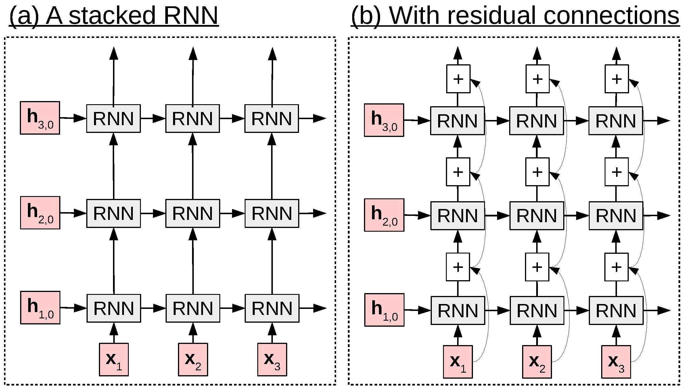
An example of (a) stacked RNNs and (b) stacked RNNs with residual connections.
One other important modification we can do to RNNs, LSTMs, GRUs, or really any other neural network layer is simple but powerful: stack multiple layers on top of each other ( (a)). For example, in a 3-layer stacked RNN, the calculation at time step t would look as follows:
$$\begin{aligned}
\bm{h}_{1,t} & = \text{RNN}_1(\bm{x}_t, \bm{h}_{1,t-1}) \nonumber \\
\bm{h}_{2,t} & = \text{RNN}_2(\bm{h}_{1,t}, \bm{h}_{2,t-1}) \nonumber \\
\bm{h}_{3,t} & = \text{RNN}_3(\bm{h}_{2,t}, \bm{h}_{3,t-1}), \nonumber\end{aligned}$$
where hn, t is the hidden state for the nth layer at time step t, and RNN(⋅) is an abbreviation for the RNN equation in . Similarly, we could substitute this function for LSTM(⋅), GRU(⋅), or any other recurrence step. The reason why stacking multiple layers on top of each other is useful is for the same reason that non-linearities proved useful in the standard neural networks introduced in : they are able to progressively extract more abstract features of the current words or sentences. For example, find evidence that in a two-layer stacked LSTM, the first layer tends to learn granular features of words such as part of speech tags, while the second layer learns more abstract features of the sentence such as voice or tense.
While stacking RNNs has potential benefits, it also has the disadvantage that it suffers from the vanishing gradient problem in the vertical direction, just as the standard RNN did in the horizontal direction. That is to say, the gradient will be back-propagated from the layer close to the output (RNN3) to the layer close to the input (RNN1), and the gradient may vanish in the process, causing the earlier layers of the network to be under-trained. A simple solution to this problem, analogous to what the LSTM does for vanishing gradients over time, is ((b)) . The idea behind these networks is simply to add the output of the previous layer directly to the result of the next layer as follows:
$$\begin{aligned}
\bm{h}_{1,t} & = \text{RNN}_1(\bm{x}_t, \bm{h}_{1,t-1}) + \bm{x}_t \nonumber \\
\bm{h}_{2,t} & = \text{RNN}_2(\bm{h}_{1,t}, \bm{h}_{2,t-1}) + \bm{h}_{1,t} \nonumber \\
\bm{h}_{3,t} & = \text{RNN}_3(\bm{h}_{2,t}, \bm{h}_{3,t-1}) + \bm{h}_{2,t}. \nonumber\end{aligned}$$
As a result, like the LSTM, there is no vanishing of gradients due to passing through the RNN(⋅) function, and even very deep networks can be learned effectively.
As the observant reader may have noticed, the previous sections have gradually introduced more and more complicated models; we started with a simple linear model, added a hidden layer, added recurrence, added LSTM, and added more layers of LSTMs. While these more expressive models have the ability to model with higher accuracy, they also come with a cost: largely expanded parameter space (causing more potential for overfitting) and more complicated operations (causing much greater potential computational cost). This section describes an effective technique to improve the stability and computational efficiency of training these more complicated networks, .
Up until this point, we have used the stochastic gradient descent learning algorithm introduced in that performs updates according to the following iterative process. This type of learning, which performs updates a single example at a time is called .
Calculate gradients of the loss Update the parameters according to this gradient
In contrast, we can also think of a algorithm, which treats the entire data set as a single unit, calculates the gradients for this unit, then only performs update after making a full pass through the data.
Calculate and accumulate gradients of the loss Update the parameters according to the accumulated gradient
These two update strategies have trade-offs.
Online training algorithms usually find a relatively good solution more quickly, as they don’t need to make a full pass through the data before performing an update.
However, at the end of training, batch learning algorithms can be more stable, as they are not overly influenced by the most recently seen training examples.
Batch training algorithms are also more prone to falling into local optima; the randomness in online training algorithms often allows them to bounce out of local optima and find a better global solution.
Minibatching is a happy medium between these two strategies. Basically, minibatched training is similar to online training, but instead of processing a single training example at a time, we calculate the gradient for n training examples at a time. In the extreme case of n = 1, this is equivalent to standard online training, and in the other extreme where n equals the size of the corpus, this is equivalent to fully batched training. In the case of training language models, it is common to choose minibatches of n = 1 to n = 128 sentences to process at a single time. As we increase the number of training examples, each parameter update becomes more informative and stable, but the amount of time to perform one update increases, so it is common to choose an n that allows for a good balance between the two.
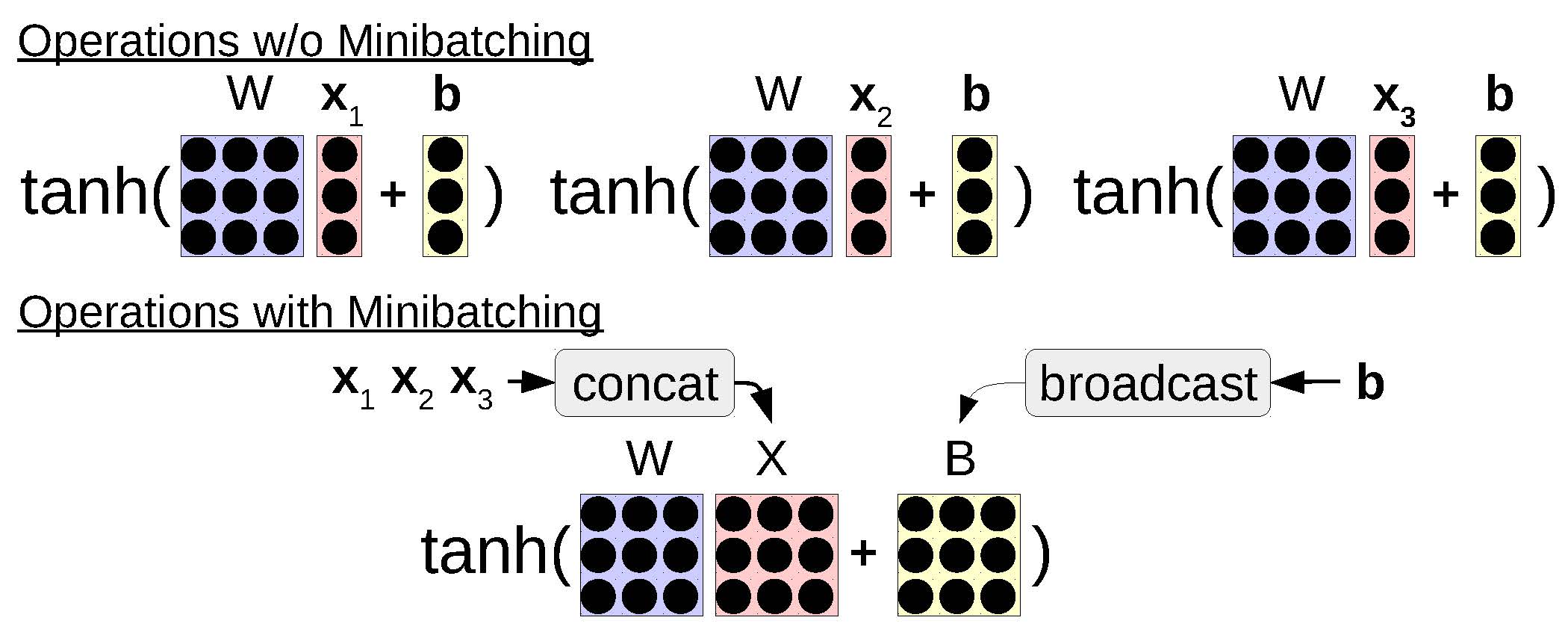
An example of combining multiple operations together when minibatching.
One other major advantage of minibatching is that by using a few tricks, it is actually possible to make the simultaneous processing of n training examples significantly faster than processing n different examples separately. Specifically, by taking multiple training examples and grouping similar operations together to be processed simultaneously, we can realize large gains in computational efficiency due to the fact that modern hardware (particularly GPUs, but also CPUs) have very efficient vector processing instructions that can be exploited with appropriately structured inputs. As shown in , common examples of this in neural networks include grouping together matrix-vector multiplies from multiple examples into a single matrix-matrix multiply or performing an element-wise operation (such as tanh) over multiple vectors at the same time as opposed to processing single vectors individually. Luckily, in DyNet, the library we are using, this is relatively easy to do, as much of the machinery for each elementary operation is handled automatically. We’ll give an example of the changes that we need to make when implementing an RNN language model below.
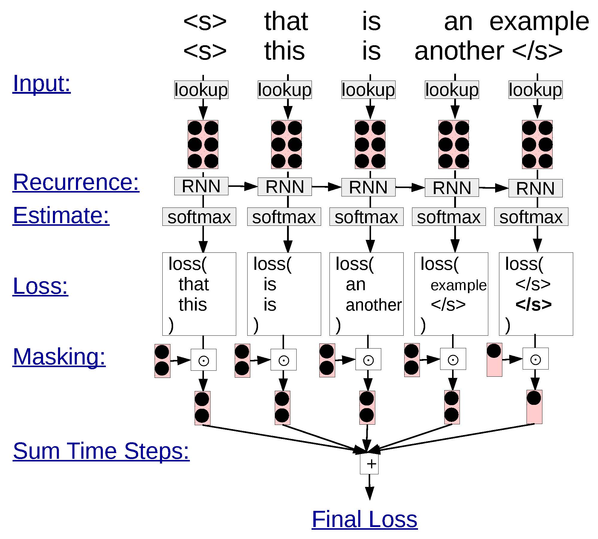
An example of minibatching in an RNN language model.
The basic idea in the batched RNN language model () is that instead of processing a single sentence, we process multiple sentences at the same time. So, instead of looking up a single word embedding, we look up multiple word embeddings (in DyNet, this is done by replacing the lookup function with the lookup_batch function, where we pass in an array of word IDs instead of a single word ID). We then run these batched word embeddings through the RNN and softmax as normal, resulting in two separate probability distributions over words in the first and second sentences. We then calculate the loss for each word (again in DyNet, replacing the pickneglogsoftmax function with the pickneglogsoftmax_batch function and pass word IDs). We then sum together the losses and use this as the loss for our entire sentence.
One sticking point, however, is that we may need to create batches with sentences of different sizes, also shown in the figure. In this case, it is common to perform and to make sure that sentences of different lengths are treated properly. Padding works by simply adding the “end-of-sentence” symbol to the shorter sentences until they are of the same length as the longest sentence in the batch. Masking works by multiplying all loss functions calculated over these padded symbols by zero, ensuring that the losses for sentence end symbols don’t get counted twice for the shorter sentences.
By taking these two measures, it becomes possible to process sentences of different lengths, but there is still a problem: if we perform lots of padding on sentences of vastly different lengths, we’ll end up wasting a lot of computation on these padded symbols. To fix this problem, it is also common to sort the sentences in the corpus by length before creating mini-batches to ensure that sentences in the same mini-batch are approximately the same size.
Because of the prevalence of RNNs in a number of tasks both on natural language and other data, there is significant interest in extensions to them. The following lists just a few other research topics that people are handling:
RNNs are surprisingly powerful tools for language, and thus many people have been interested in what exactly is going on inside them. demonstrate ways to visualize the internal states of LSTM networks, and find that some nodes are in charge of keeping track of length of sentences, whether a parenthesis has been opened, and other salietn features of sentences. show ways to analyze and visualize which parts of the input are contributing to particular decisions made by an RNN-based model, by back-propagating information through the network.
There are also quite a few other recurrent network architectures. perform an interesting study where they ablate various parts of the LSTM and attempt to find the best architecture for particular tasks. take it a step further, explicitly training the model to find the best neural network architecture.
In the exercise for this chapter, we will construct a recurrent neural network language model using LSTMs.
Writing the program will entail:
Writing a function such as lstm_step or gru_step that takes the input of the previous time step and updates it according to the appropriate equations. For reference, in DyNet, the componentwise multiply and sigmoid functions are dy.cmult and dy.logistic respectively.
Adding this function to the previous neural network language model and measuring the effect on the held-out set.
Ideally, implement mini-batch training by using the functionality implemented in DyNet, lookup_batch and pickneglogsoftmax_batch.
Language modeling accuracy should be measured in the same way as previous exercises and compared with the previous models.
Potential improvements to the model include: Measuring the speed/stability improvements achieved by mini-batching. Comparing the differences between recurrent architectures such as RNN, GRU, or LSTM.
See https://en.wikipedia.org/wiki/Russian_grammar for an overview.↩
This is particularly detrimental in the case where we receive a loss only once at the end of the sentence, like the example above. One real-life example of such a scenario is document classification, and because of this, RNNs have been less successful in this task than other methods such as convolutional neural networks, which do not suffer from the vanishing gradient problem . It has been shown that pre-training an RNN as a language model before attempting to perform classification can help alleviate this problem to some extent .↩
To be more accurate, the sigmoid function is actually any mathematical function having an s-shaped curve, so the tanh function is also a type of sigmoid function. The logistic function is also a slightly broader class of functions $f(x) = \frac{L}{1+\exp(-k(x-x_0))}$. However, in the machine learning literature, the “sigmoid” is usually used to refer to the particular variety in .↩
In actuality it ⊙ ut is also affected by ct − 1, and thus $\frac{d\bm{c}_t}{d\bm{c}_{t-1}}$ is not exactly one, but the effect is relatively indirect. Especially for vector elements with it close to zero, the effect will be minimal.↩