From to , we focused on the language modeling problem of calculating the probability P(E) of a sequence E. In this section, we return to the statistical machine translation problem (mentioned in ) of modeling the probability P(E ∣ F) of the output E given the input F.

Encoder-decoder Models

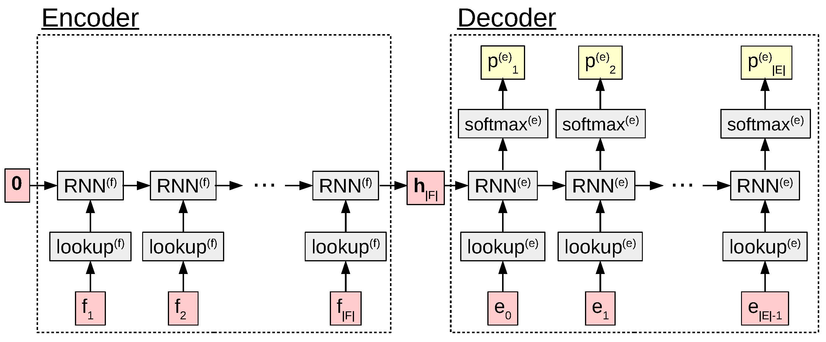
The first model that we will cover is called an model . The basic idea of the model is relatively simple: we have an RNN language model, but before starting calculation of the probabilities of E, we first calculate the initial state of the language model using another RNN over the source sentence F. The name “encoder-decoder” comes from the idea that the first neural network running over F “encodes” its information as a vector of real-valued numbers (the hidden state), then the second neural network used to predict E “decodes” this information into the target sentence.

A computation graph of the encoder-decoder model.

If the encoder is expressed as RNN^(f)(⋅), the decoder is expressed as RNN^(e)(⋅), and we have a softmax that takes RNN^(e)’s hidden state at time step t and turns it into a probability, then our model is expressed as follows (also shown in ):
$$\begin{aligned} \bm{m}^{(f)}_t & = M^{(f)}_{\cdot,f_t} \nonumber \\ \bm{h}^{(f)}_t & = \begin{cases} \text{RNN}^{(f)}(\bm{m}^{(f)}_t, \bm{h}^{(f)}_{t-1}) & t \ge 1, \\ \bm{0} & \mbox{otherwise}. \\ \end{cases} \nonumber \\ \bm{m}^{(e)}_t & = M^{(e)}_{\cdot,e_{t-1}} \nonumber \\ \bm{h}^{(e)}_t & = \begin{cases} \text{RNN}^{(e)}(\bm{m}^{(e)}_t, \bm{h}^{(e)}_{t-1}) & t \ge 1, \\ \bm{h}^{(f)}_{|F|} & \mbox{otherwise}. \\ \end{cases} \nonumber \\ \bm{p}^{(e)}_t & = \text{softmax}(W_{hs} \bm{h}^{(e)}_t + b_s) \label{eq:encdec:softmax}\end{aligned}$$
In the first two lines, we look up the embedding m_t^(f) and calculate the encoder hidden state h_t^(f) for the tth word in the source sequence F. We start with an empty vector h₀^(f) = 0, and by h_|F|^(f), the encoder has seen all the words in the source sentence. Thus, this hidden state should theoretically be able to encode all of the information in the source sentence.

In the decoder phase, we predict the probability of word e_t at each time step. First, we similarly look up m_t^(e), but this time use the previous word e_t − 1, as we must condition the probability of e_t on the previous word, not on itself. Then, we run the decoder to calculate h_t^(e). This is very similar to the encoder step, with the important difference that h₀^(e) is set to the final state of the encoder h_|F|^(f), allowing us to condition on F. Finally, we calculate the probability p_t^(e) by using a softmax on the hidden state h_t^(e).

While this model is quite simple (only 5 lines of equations), it gives us a straightforward and powerful way to model P(E ∣ F). In fact, have shown that a model that follows this basic pattern is able to perform translation with similar accuracy to heavily engineered systems specialized to the machine translation task (although it requires a few tricks over the simple encoder-decoder that we’ll discuss in later sections: beam search (), a different encoder (), and ensembling ()). and ensembling ()).

Generating Output

At this point, we have only mentioned how to create a probability model P(E ∣ F) and haven’t yet covered how to actually generate translations from it, which we will now cover in the next section. In general, when we generate output we can do so according to several criteria:

Which of these methods we will choose will depend on our application, so we will discuss some use cases along with the algorithms themselves.

Random Sampling

First, is useful in cases where we may want to get a variety of outputs for a particular input. One example of a situation where this is useful would be in a sequence-to-sequence model for a dialog system, where we would prefer the system to not always give the same response to a particular user input to prevent monotony. Luckily, in models like the encoder-decoder above, it is simple to exactly generate samples from the distribution P(E ∣ F) using a method called . Ancestral sampling works by sampling variable values one at a time, gradually conditioning on more context, so at time step t, we will sample a word from the distribution $P(e_t \mid \hat{e}_{1}^{t-1})$. In the encoder-decoder model, this means we simply have to calculate p_t according to the previously sampled inputs, leading to the simple generation algorithm in .

One thing to note is that sometimes we also want to know the probability of the sentence that we sampled. For example, given a sentence $\hat{E}$ generated by the model, we might want to know how certain the model is in its prediction. During the sampling process, we can calculate $P(\hat{E} \mid F) = \prod_{t}^{|\hat{E}|} P(\hat{e}_t \mid F,\hat{E}_1^{t-1})$ incrementally by stepping along and multiplying together the probabilities of each sampled word. However, as we remember from the discussion of probability vs. log probability in , using probabilities as-is can result in very small numbers that cause numerical precision problems on computers. Thus, when calculating the full-sentence probability it is more common to instead add together log probabilities for each word, which avoids this problem.

Calculate m_t^(f) and h_t^(f) Set $\hat{e}_0=$“$\sentbegin$” and t ← 0 t ← t + 1 Calculate m_t^(e), h_t^(e), and p_t^(e) from $\hat{e}_{t-1}$ Sample $\hat{e}_t$ according to p_t^(e)

Greedy 1-best Search

Next, let’s consider the problem of generating a 1-best result. This variety of generation is useful in machine translation, and most other applications where we simply want to output the translation that the model thought was best. The simplest way of doing so is , in which we simply calculate p_t at every time step, select the word that gives us the highest probability, and use it as the next word in our sequence. In other words, this algorithm is exactly the same as , with the exception that on Line 9, instead of sampling $\hat{e}_t$ randomly according to p_t^(e), we instead choose the max: $\hat{e}_t = \argmax{i} p^{(e)}_{t,i}$.

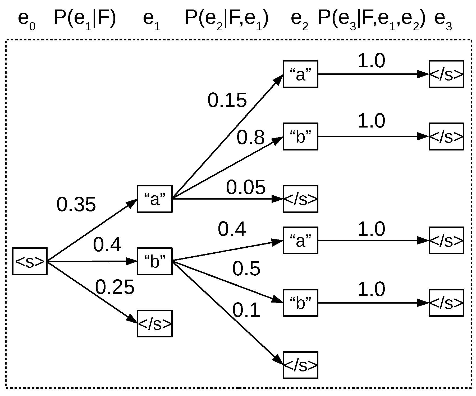
A search graph where greedy search fails.

Interestingly, while ancestral sampling exactly samples outputs from the distribution according to P(E ∣ F), greedy search is not guaranteed to find the translation with the highest probability. An example of a case in which this is true can be found in the graph in , which is an example of search graph with a vocabulary of $\{\text{a}, \text{b}, \sentend\}$.¹ As an exercise, I encourage readers to find the true 1-best (or n-best) sentence according to the probability P(E ∣ F) and the probability of the sentence found according to greedy search and confirm that these are different.

An example of beam search with b = 2. Numbers next to arrows are log probabilities for a single word logP(e_t ∣ F, e₁^t − 1), while numbers above nodes are log probabilities for the entire hypothesis up until this point.

Beam Search

One way to solve this problem is through the use of . Beam search is similar to greedy search, but instead of considering only the one best hypothesis, we consider b best hypotheses at each time step, where b is the “width” of the beam. An example of beam search where b = 2 is shown in (note that we are using log probabilities here because they are more conducive to comparing hypotheses over the entire sentence, as mentioned before). In the first time step, we expand hypotheses for e₁ corresponding to all of the three words in the vocabulary, then keep the top two (“b” and “a”) and delete the remaining one (“$\sentend$”). In the second time step, we expand hypotheses for e₂ corresponding to the continuation of the first hypotheses for all words in the vocabulary, temporarily creating b * |V| active hypotheses. These active hypotheses are also pruned down to the b active hypotheses (“a b” and “b b”). This process of calculating scores for b * |V| continuations of active hypotheses, then pruning back down to the top b, is continued until the end of the sentence.

One thing to be careful about when generating sentences using models, such as neural machine translation, where $P(E \mid F) = \prod_t^{|E|} P(e_t \mid F,e_1^{t-1})$ is that they tend to prefer shorter sentences. This is because every time we add another word, we multiply in another probability, reducing the probability of the whole sentence. As we increase the beam size, the search algorithm gets better at finding these short sentences, and as a result, beam search with a larger beam size often has a significant towards these shorter sentences.

There have been several attempts to fix this length bias problem. For example, it is possible to put a prior probability on the length of the sentence given the length of the previous sentence P(|E|∣|F|), and multiply this with the standard sentence probability P(E ∣ F) at decoding time :
$$\hat{E} = \argmax{E} \log P(|E| \mid |F|) + \log P(E \mid F).$$
This prior probability can be estimated from data, and simply estimate this using a multinomial distribution learned on the training data:
$$P(|E| \mid |F|) = \frac{c(|E|,|F|)}{c(|F|)}.$$
A more heuristic but still widely used approach normalizes the log probability by the length of the target sentence, effectively searching for the sentence that has the highest average log probability per word :
$$\hat{E} = \argmax{E} \log P(E \mid F) / |E|.$$

Other Ways of Encoding Sequences

In , we described a model that works by encoding sequences linearly, one word at a time from left to right. However, this may not be the most natural or effective way to turn the sentence F into a vector h. In this section, we’ll discuss a number of different ways to perform encoding that have been reported to be effective in the literature.

Reverse and Bidirectional Encoders

First, have proposed a . In this method, we simply run a standard linear encoder over F, but instead of doing so from left to right, we do so from right to left.
$$\overleftarrow{\bm{h}}^{(f)}_t = \begin{cases} \overleftarrow{\text{RNN}}^{(f)}(\bm{m}^{(f)}_t, \overleftarrow{\bm{h}}^{(f)}_{t+1}) & t \le |F|, \\ \bm{0} & \mbox{otherwise}. \\ \end{cases}$$
The motivation behind this method is that for pairs of languages with similar ordering (such as English-French, which the authors experimented on), the words at the beginning of F will generally correspond to words at the beginning of E. Assuming the extreme case that words with identical indices correspond to each-other (e.g. f₁ corresponds to e₁, f₂ to e₂, etc.), the distance between corresponding words in the linear encoding and decoding will be |F|, as shown in (a). Remembering the vanishing gradient problem from , this means that the RNN has to propagate the information across |F| time steps before making a prediction, a difficult feat. At the beginning of training, even RNN variants such as LSTMs have trouble, as they have to essentially “guess” what part of the information encoded in their hidden state is being used without any prior bias.

The distances between words with the same index in the forward and reverse decoders.

Reversing the encoder helps solve this problem by reducing the length of dependencies for a subset of the words in the sentence, specifically the ones at the beginning of the sentences. As shown in (b), the length of the dependency for f₁ and e₁ is 1, and subsequent pairs of f_t and e_t have a distance of 2t − 1. During learning, the model can “latch on” to these short-distance dependencies and use them as a way to bootstrap the model training, after which it becomes possible to gradually learn the longer dependencies for the words at the end of the sentence. In , this proved critical to learn effective models in the encoder-decoder framework.

However, this approach of reversing the encoder relies on the strong assumption that the order of words in the input and output sequences are very similar, or at least that the words at the beginning of sentences are the same. This is true for languages like English and French, which share the same “subject-verb-object (SVO)” word ordering, but may not be true for more typologically distinct languages. One type of encoder that is slightly more robust to these differences is the . In this method, we use two different encoders: one traveling forward and one traveling backward over the input sentence
$$\begin{aligned} \overrightarrow{\bm{h}}^{(f)}_t & = \begin{cases} \overrightarrow{\text{RNN}}^{(f)}(\bm{m}^{(f)}_t, \overrightarrow{\bm{h}}^{(f)}_{t+-}) & t \ge 1, \\ \bm{0} & \mbox{otherwise}. \\ \end{cases} \\ \overleftarrow{\bm{h}}^{(f)}_t & = \begin{cases} \overleftarrow{\text{RNN}}^{(f)}(\bm{m}^{(f)}_t, \overleftarrow{\bm{h}}^{(f)}_{t+1}) & t \le |F|, \\ \bm{0} & \mbox{otherwise}. \\ \end{cases}\end{aligned}$$
which are then combined into the initial vector h₀^(e) for the decoder RNN. This combination can be done by simply concatenating the two final vectors $\overrightarrow{\bm{h}}_{|F|}$ and $\overleftarrow{\bm{h}}_{1}$. However, this also requires that the size of the vectors for the decoder RNN be exactly equal to the combined size of the two encoder RNNs. As a more flexible alternative, we can add an additional parameterized hidden layer between the encoder and decoder states, which allows us to convert the bidirectional encoder states into an appropriately-sized state for the decoder:
$$\bm{h}^{(e)}_0 = \tanh(W_{\overrightarrow{f}e}\overrightarrow{\bm{h}}_{|F|} + W_{\overleftarrow{f}e}\overleftarrow{\bm{h}}_{1} + \bm{b}_e).$$

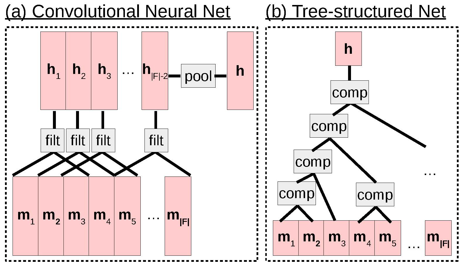
Examples of convolutional and tree-structured networks.

Convolutional Neural Networks

In addition, there are also methods for decoding that move beyond a simple linear view of the input sentence. For example, (CNNs; ), (a)) are a variety of neural net that combines together information from spatially or temporally local segments. They are most widely applied to image processing but have also been used for speech processing, as well as the processing of textual sequences. While there are many varieties of CNN-based models of text (e.g. ), here we will show an example from . This model has n with a width w that are passed incrementally over w-word segments of the input. Specifically, given an embedding matrix M of width |F|, we generate a hidden layer matrix H of width |F|−w + 1, where each column of the matrix is equal to
h_t = Wconcat(m_t, m_t + 1, …, m_{t + w − 1})
where W ∈ ℝ^{n × w|m|} is a matrix where the ith row represents the parameters of filter i that will be multiplied by the embeddings of w consecutive words. If w = 3, we can interpret this as h₁ extracting a vector of features for f₁³, h₂ as extracting a vector of features for f₂⁴, etc. until the end of the sentence.

Finally, we perform a operation that converts this matrix H (which varies in width according to the sentence length) into a single vector h (which is fixed-size and can thus be used in down-stream processing). Examples of pooling operations include average, max, and k-max .

Compared to RNNs and their variants, CNNs have several advantages and disadvantages:

In general, CNNs have been found to be quite effective for text classification, where it is more important to pick out the most indicative features of the text and there is less of an emphasis on getting an overall view of the content . There have also been some positive results reported using specific varieties of CNNs for sequence-to-sequence modeling .

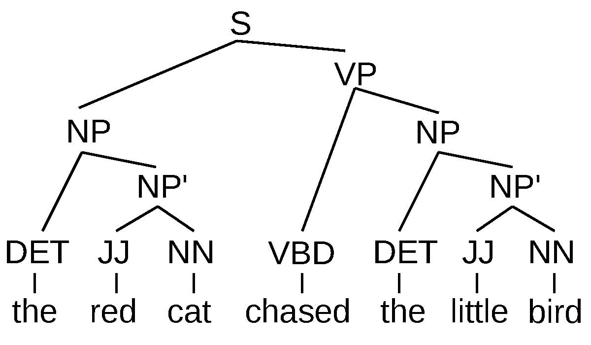
An example of a syntax tree for a sentence showing the sentence structure and phrase types (DET=“determiner”, JJ=“adjective”, NN=“noun”, VBD=“past tense verb”, NP=“noun phrase”, NP’=“part of a noun phrase”, VP=“verb phrase”, S=“sentence”).

Tree-structured Networks

Finally, one other popular form of encoder that is widely used in a number of tasks are (, (b)). The basic idea behind these networks is that the way to combine the information from each particular word is guided by some sort of structure, usually the syntactic structure of the sentence, an example of which is shown in . The reason why this is intuitively useful is because each syntactic phrase usually also corresponds to a coherent semantic unit. Thus, performing the calculation and manipulation of vectors over these coherent units will be more appropriate compared to using random substrings of words, like those used by CNNs.

For example, let’s say we have the phrase “the red cat chased the little bird” as shown in the figure. In this case, following a syntactic tree would ensure that we calculate vectors for coherent units that correspond to a grammatical phrase such as “chased” and “the little bird”, and combine these phrases together one by one to obtain the meaning of larger coherent phrase such as “chased the little bird”. By doing so, we can take advantage of the fact that language is , with the meaning of a more complex phrase resulting from regular combinations and transformation of smaller constituent phrases . By taking this linguistically motivated and intuitive view of the sentence, we hope will help the neural networks learn more generalizable functions from limited training data.

Perhaps the most simple type of tree-structured network is the proposed by . This network has very strong parallels to standard RNNs, but instead of calculating the hidden state h_t at time t from the previous hidden state h_t − 1 as follows:
h_t = tanh(W_xhx_t + W_hhh_t − 1 + b_h),
we instead calculate the hidden state of the parent node h_p from the hidden states of the left and right children, h_l and h_r respectively:
h_p = tanh(W_xpx_t + W_lph_l + W_rph_r + b_p).
Thus, the representation for each node in the tree can be calculated in a bottom-up fashion.

Like standard RNNs, these recursive networks suffer from the vanishing gradient problem. To fix this problem there is an adaptation of LSTMs to tree-structured networks, fittingly called , which fixes this vanishing gradient problem. There are also a wide variety of other kinds of tree-structured composition functions that interested readers can explore . Also of interest is the study by , which examines the various tasks in which tree structures are necessary or unnecessary for NLP.

Ensembling Multiple Models

One other method that is widely used in encoder-decoders, or other models of translation is : the combination of the prediction of multiple independently trained models to improve the overall prediction results. The intuition behind ensembling is that different models will make different mistakes, and that on average it is more common for models to agree when the answer is correct than when it is mistaken. Thus, if we combine multiple models together, it becomes possible to smooth over these mistakes, finding the correct answer more often.

The first step in ensembling encoder-decoder models is to independently train N different models P₁(⋅),P₂(⋅),…,P_N(⋅), for example, by randomly initializing the weights of the neural network differently before training. Next, during search, at each time step we calculate the probability of the next word as the average probability of the N models:
$$P(e_t \mid F, e_1^{t-1}) = \frac{1}{N} \sum_{i=1}^{N} P_i(e_t \mid F, e_1^{t-1}).$$
This probability is used in searching for our hypotheses.

Exercise

In the exercise for this chapter, we will create an encoder-decoder translation model and make it possible to generate translations.

Potential improvements to the model include: Implementing beam search and comparing the results with greedy search. Implementing an alternative encoder. Implementing ensembling.

In reality, we will never have a probability of exactly $P(e_t=\sentend \mid F,e_1^{t-1})=1.0$, but for illustrative purposes, we show this here.↩

7 Neural Encoder-Decoder Models