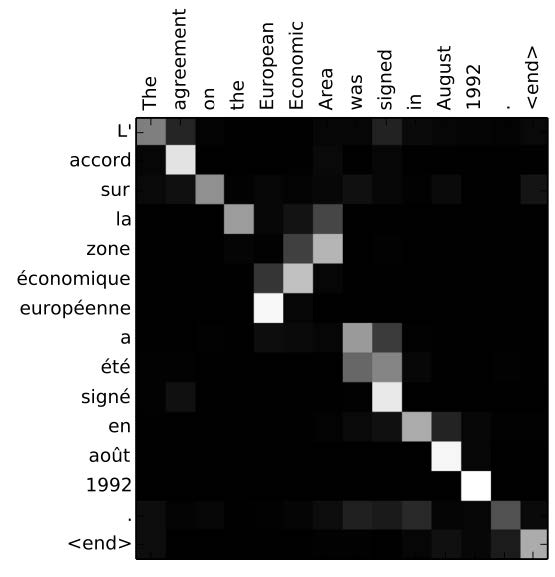
An example of attention from . English is the source, French is the target, and a higher attention weight when generating a particular target word is indicated by a lighter color in the matrix.
In the past chapter, we described a simple model for neural machine translation, which uses an encoder to encode sentences as a fixed-length vector. However, in some ways, this view is overly simplified, and by the introduction of a powerful mechanism called , we can overcome these difficulties. This section describes the problems with the encoder-decoder architecture and what attention does to fix these problems.
Theoretically, a sufficiently large and well-trained encoder-decoder model should be able to perform machine translation perfectly. As mentioned in , neural networks are universal function approximators, meaning that they can express any function that we wish to model, including a function that accurately predicts our predictive probability for the next word P(et ∣ F, e1t − 1). However, in practice, it is necessary to learn these functions from limited data, and when we do so, it is important to have a proper – an appropriate model structure that allows the network to learn to model accurately with a reasonable amount of data.
There are two things that are worrying about the standard encoder-decoder architecture. The first was described in the previous section: there are long-distance dependencies between words that need to be translated into each other. In the previous section, this was alleviated to some extent by reversing the direction of the encoder to bootstrap training, but still, a large number of long-distance dependencies remain, and it is hard to guarantee that we will learn to handle these properly.
The second, and perhaps more, worrying aspect of the encoder-decoder is that it attempts to store information sentences of any arbitrary length in a hidden vector of fixed size. In other words, even if our machine translation system is expected to translate sentences of lengths from 1 word to 100 words, it will still use the same intermediate representation to store all of the information about the input sentence. If our network is too small, it will not be able to encode all of the information in the longer sentences that we will be expected to translate. On the other hand, even if we make the network large enough to handle the largest sentences in our inputs, when processing shorter sentences, this may be overkill, using needlessly large amounts of memory and computation time. In addition, because these networks will have large numbers of parameters, it will be more difficult to learn them in the face of limited data without encountering problems such as overfitting.
The remainder of this section discusses a more natural way to solve the translation problem with neural networks: attention.
The basic idea of attention is that instead of attempting to learn a single vector representation for each sentence, we instead keep around vectors for every word in the input sentence, and reference these vectors at each decoding step. Because the number of vectors available to reference is equivalent to the number of words in the input sentence, long sentences will have many vectors and short sentences will have few vectors. As a result, we can express input sentences in a much more efficient way, avoiding the problems of inefficient representations for encoder-decoders mentioned in the previous section.
First we create a set of vectors that we will be using as this variably-lengthed representation. To do so, we calculate a vector for every word in the source sentence by running an RNN in both directions:
$$\begin{aligned}
% \label{eq:encode}
\overrightarrow{\bm{h}}^{(f)}_j = \text{RNN}( \text{embed}(f_j), \overrightarrow{\bm{h}}^{(f)}_{j-1} ) \\
\overleftarrow{\bm{h}}^{(f)}_j = \text{RNN}( \text{embed}(f_j), \overleftarrow{\bm{h}}^{(f)}_{j+1} ).\end{aligned}$$
Then we concatenate the two vectors $\overrightarrow{\bm{h}}^{(f)}_j$ and $\overleftarrow{\bm{h}}^{(f)}_j$ into a bidirectional representation hj(f)
$$\bm{h}^{(f)}_j = [\overleftarrow{\bm{h}}^{(f)}_j; \overrightarrow{\bm{h}}^{(f)}_j].$$
We can further concatenate these vectors into a matrix:
H(f) = concat_col(h1(f), …, h|F|(f)).
This will give us a matrix where every column corresponds to one word in the input sentence.
An example of attention from . English is the source, French is the target, and a higher attention weight when generating a particular target word is indicated by a lighter color in the matrix.
However, we are now faced with a difficulty. We have a matrix H(f) with a variable number of columns depending on the length of the source sentence, but would like to use this to compute, for example, the probabilities over the output vocabulary, which we only know how to do (directly) for the case where we have a vector of input. The key insight of attention is that we calculate a vector αt that can be used to combine together the columns of H into a vector ct
ct = H(f)αt.
αt is called the , and is generally assumed to have elements that are between zero and one and add to one.
The basic idea behind the attention vector is that it is telling us how much we are “focusing” on a particular source word at a particular time step. The larger the value in αt, the more impact a word will have when predicting the next word in the output sentence. An example of how this attention plays out in an actual translation example is shown in , and as we can see the values in the alignment vectors generally align with our intuition.
The next question then becomes, from where do we get this αt? The answer to this lies in the decoder RNN, which we use to track our state while we are generating output. As before, the decoder’s hidden state ht(e) is a fixed-length continuous vector representing the previous target words e1t − 1, initialized as h0(e) = h|F|+1(f). This is used to calculate a context vector ct that is used to summarize the source attentional context used in choosing target word et, and initialized as c0 = 0.
First, we update the hidden state to ht(e) based on the word representation and context vectors from the previous target time step
ht(e) = enc([embed(et − 1);ct − 1],ht − 1(e)).
Based on this ht(e), we calculate an at, with each element equal to
at, j = attn_score(hj(f), ht(e)).
attn_score(⋅) can be an arbitrary function that takes two vectors as input and outputs a score about how much we should focus on this particular input word encoding hj(f) at the time step ht(e). We describe some examples at a later point in .
We then normalize this into the actual attention vector itself by taking a softmax over the scores:
αt = softmax(at).
This attention vector is then used to weight the encoded representation H(f) to create a context vector ct for the current time step, as mentioned in .
We now have a context vector ct and hidden state ht(e) for time step t, which we can pass on down to downstream tasks. For example, we can concatenate both of these together when calculating the softmax distribution over the next words:
pt(e) = softmax(Whs[ht(e); ct]+bs).
It is worth noting that this means that the encoding of each source word hj(f) is considered much more directly in the calculation of output probabilities. In contrast to the encoder-decoder, where the encoder-decoder will only be able to access information about the first encoded word in the source by passing it over |F| time steps, here the source encoding is accessed (in a weighted manner) through the context vector .
This whole, rather involved, process is shown in .
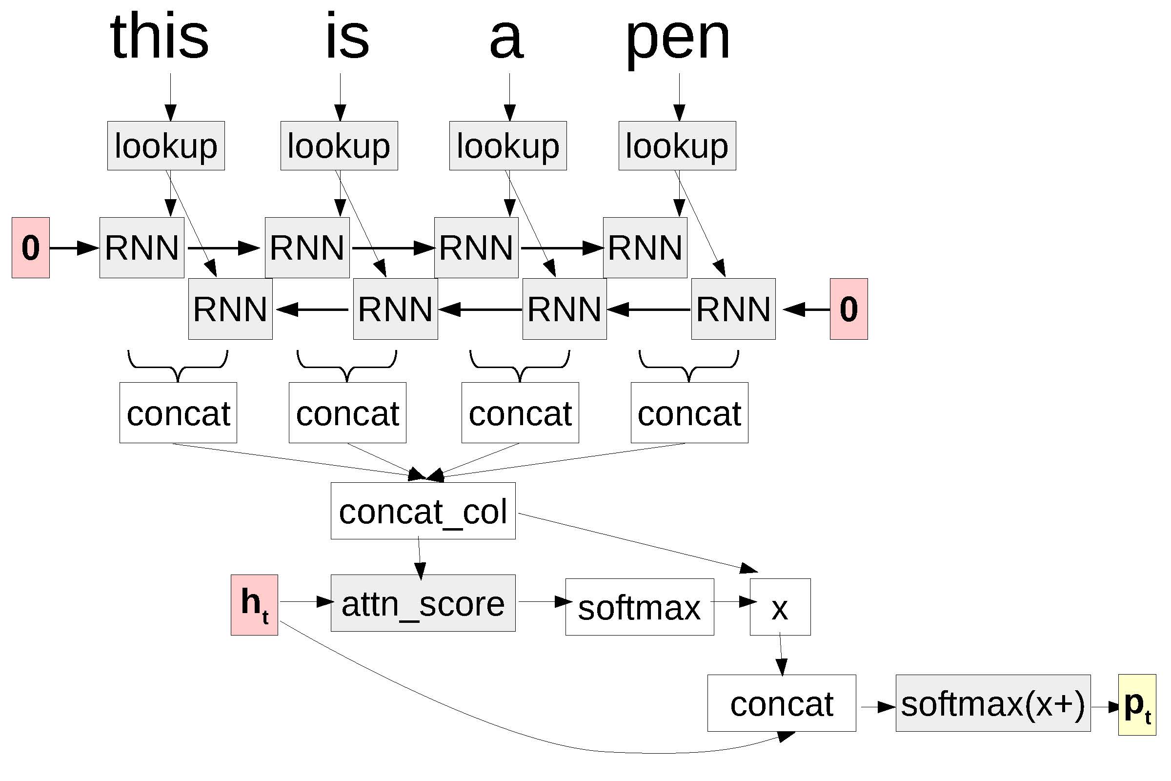
A computation graph for attention.
As mentioned in , the final missing piece to the puzzle is how to calculate the attention score at, j.
test three different attention functions, all of which have their own merits:
This is the simplest of the functions, as it simply calculates the similarity between ht(e) and hj(f) as measured by the dot product:
attn_score(hj(f), ht(e)):=hj(f)⊺ht(e).
This model has the advantage that it adds no additional parameters to the model. However, it also has the intuitive disadvantage that it forces the input and output encodings to be in the same space (because similar ht(e) and hj(f) must be close in space in order for their dot product to be high). It should also be noted that the dot product can be calculated efficiently for every word in the source sentence by instead defining the attention score over the concatenated matrix H(f) as follows:
attn_score(H(f), ht(e)):=Hj(f)⊺ht(e).
Combining the many attention operations into one can be useful for efficient impementation, especially on GPUs. The following attention functions can also be calculated like this similarly.
One slight modification to the dot product that is more expressive is the . This function helps relax the restriction that the source and target embeddings must be in the same space by performing a linear transform parameterized by Wa before taking the dot product:
attn_score(hj(f), ht(e)):=hj(f)⊺Waht(e).
This has the advantage that if Wa is not a square matrix, it is possible for the two vectors to be of different sizes, so it is possible for the encoder and decoder to have different dimensions. However, it does introduce quite a few parameters to the model (|h(f)|×|h(e)|), which may be difficult to train properly.
Finally, it is also possible to calculate the attention score using a multi-layer perceptron, which was the method employed by in their original implementation of attention:
attn_score(ht(e), hj(f)):=wa2⊺tanh(Wa1[ht(e); hj(f)]),
where Wa1 and wa2 are the weight matrix and vector of the first and second layers of the MLP respectively. This is more flexible than the dot product method, usually has fewer parameters than the bilinear method, and generally provides good results.
In addition to these methods above, which are essentially the defacto-standard, there are a few more sophisticated methods for calculating attention as well. For example, it is possible to use recurrent neural networks , tree-structured networks based on document structure , convolutional neural networks , or structured models to calculate attention.
One pleasant side-effect of attention is that it not only increases translation accuracy, but also makes it easier to tell which words are translated into which words in the output. One obvious consequence of this is that we can draw intuitive graphs such as the one shown in , which aid error analysis.
Another advantage is that it also becomes possible to handle unknown words in a more elegant way, performing . The idea of this method is simple, every time our decoder chooses the unknown word token $\sentunk$ in the output, we look up the source word with the highest attention weight at this time step, and output that word instead of the unknown token $\sentunk$. If we do so, at least the user can see which words have been left untranslated, which is better than seeing them disappear altogether or be replaced by a placeholder.
It is also common to use alignment models such as those in to obtain a translation dictionary, then use this to aid unknown word replacement even further. It is also common to use alignment models such as those described in to obtain a translation dictionary, then use this to aid unknown word replacement even further. Specifically, instead of copying the word as-is into the output, if the chosen source word is f, we output the word with the highest translation probability Pdict(e ∣ f). This allows words that are included in the dictionary to be mapped into their most-frequent counterpart in the target language.
Because of the importance of attention in modern NMT systems, there have also been a number of proposals to improve accuracy of estimating the attention itself through the introduction of intuitively motivated prior probabilities. propose several methods to incorporate biases into the training of the model to ensure that the attention weights match our belief of what alignments between languages look like.
These take several forms, and are heavily inspired by the alignment models that will be explained in . These take several forms, and are heavily inspired by the alignment models used in more traditional SMT systems such as those proposed by . These models can be briefly summarized as:
If two languages have similar word order, then it is more likely that alignments should fall along the diagonal. This is demonstrated strongly in . It is possible to encourage this behavior by adding a prior probability over attention that makes it easier for things near the diagonal to be aligned.
In most languages, we can assume that most of the time if two words in the target are contiguous, the aligned words in the source will also be contiguous. For example, in , this is true for all contiguous pairs of English words except “the, European” and “Area, was”. To take advantage of this property, it is possible to impose a prior that discourages large jumps and encourages local steps in attention. A model that is similar in motivation, but different in implementation, is the model , which selects which part of the source sentence to focus on using the neural network itself.
We can assume that some words will be translated into a certain number words in the other langauge. For example, the English word “cats” will be translated into two words “les chats” in French. Priors on fertility takes advantage of this fact by giving the model a penalty when particular words are not attended too much, or attended to too much. In fact one of the major problems with poorly trained neural MT systems is that they repeat the same word over and over, or drop words, a violation of this fertility constraint. Because of this, several other methods have been proposed to incorporate coverage in the model itself , or as a constraint during the decoding process .
Finally, we expect that words that are aligned when performing translation from F to E should also be aligned when performing translation from E to F. This can be enforced by training two models in parallel, and enforcing constraints that the alignment matrices look similar in both directions.
experiment extensively with these approaches, and find that the bilingual symmetry constraint is particularly effective among the various methods.
This section outlines some further directions for reading more about improvements to attention:
As shown in , standard attention uses a soft combination of various contents. There are also methods for hard attention that make a hard binary decision about whether to focus on a particular context, with motivations ranging from learning explainable models , to processing text incrementally .
In addition, sometimes we have hand-annotated data showing us true alignments for a particular language pair. It is possible to train attentional models using this data by defining a loss function that penalizes the model when it does not predict these alignments correctly .
Finally, there are other ways of accessing relevant information other than attention. propose a method using , which have a separate set of memory that can be written to or read from as the processing continues.
In the exercise for this chapter, we will create code to train and generate translations with an attentional neural MT model.
Writing the program will entail extending your encoder-decoder code to add attention. You can then generate translations and compare them to others.
Extend your encoder-decoder code to add attention.
On the training set, write code to calculate the loss function and perform training.
On the development set, generate translations using greedy search.
Evaluate these translations, either manually or automatically.
It is also highly recommended, but not necessary, that you attempt to implement unknown word replacement.
Potential improvements to the model include implementing any of the improvements to attention mentioned in or .