胶囊之间的动态路由

摘要

胶囊是一组神经元，其活动向量表示特定类型实体（例如对象或对象部分）的实例化参数。 我们使用活动向量的长度来表示实体存在的概率，并使用其方向来表示实例化参数。 某一级别的活动胶囊通过变换矩阵对更高级别胶囊的实例化参数进行预测。 当多个预测一致时，更高级别的胶囊就会被激活。 我们证明，经过区分训练的多层胶囊系统在 MNIST 上实现了最先进的性能，并且在识别高度重叠的数字方面比卷积网络要好得多。 为了实现这些结果，我们使用迭代路由协议机制：较低级别的胶囊更喜欢将其输出发送到较高级别的胶囊，其活动向量与来自较低级别胶囊的预测具有较大的标量积。

1简介

人类视觉通过使用仔细确定的固定点序列来忽略不相关的细节，以确保仅以最高分辨率处理光学阵列的一小部分。 内省对于理解我们对场景的了解有多少来自注视序列以及我们从单个注视中收集了多少信息来说是一个糟糕的指导，但在本文中，我们将假设单个注视给我们带来的不仅仅是单个注视。识别的对象及其属性。 我们假设我们的多层视觉系统在每个注视点上创建一个类似解析树的结构，并且我们忽略了这些单注视点解析树如何在多个注视点上协调的问题。

解析树通常是通过动态分配内存来动态构建的。 然而，根据Hinton等人（2000），我们假设，对于单个固定，解析树是从固定的多层神经网络中雕刻出来的，就像从岩石中雕刻出雕塑一样。 每层将被分为许多称为“胶囊”的神经元小组(Hinton 等人（2011）)，解析树中的每个节点将对应于一个活动胶囊。 使用迭代路由过程，每个活动胶囊将选择上层中的一个胶囊作为其在树中的父胶囊。 对于更高层次的视觉系统，这个迭代过程将解决将部分分配给整体的问题。

活动胶囊内神经元的活动代表图像中存在的特定实体的各种属性。 这些属性可以包括许多不同类型的实例化参数，例如姿势（位置、大小、方向）、变形、速度、反照率、色调、纹理等。一个非常特殊的属性是图像中实例化实体的存在。 表示存在的一种明显方法是使用单独的逻辑单元，其输出是实体存在的概率。 在本文中，我们探索了一种有趣的替代方案，即使用实例化参数向量的总长度来表示实体的存在，并强制向量的方向来表示实体的属性. 我们通过应用非线性来确保胶囊的矢量输出的长度不能超过 $1$，该非线性使矢量的方向保持不变但缩小其幅度。

胶囊的输出是一个向量，这一事实使得可以使用强大的动态路由机制来确保胶囊的输出发送到上层中适当的父级。 最初，输出被路由到所有可能的父级，但通过总和为 $1$ 的耦合系数按比例缩小。 对于每个可能的父代，胶囊通过将其自身的输出乘以权重矩阵来计算“预测向量”。 如果该预测向量与可能的父对象的输出具有较大的标量积，则存在自上而下的反馈，该反馈会增加该父对象的耦合系数并减少其他父对象的耦合系数。 这增加了胶囊对该父代的贡献，从而进一步增加了胶囊预测与父代输出的标量积。 这种类型的“协议路由”应该比最大池化实现的非常原始的路由形式有效得多，最大池化允许一层中的神经元忽略该层中本地池中除了最活跃的特征检测器之外的所有特征检测器以下。 我们证明了我们的动态路由机制是实现分割高度重叠对象所需的“解释”的有效方法。

卷积神经网络 (CNN) 使用学习到的特征检测器的翻译副本。 这使得他们能够将在图像中的一个位置获取的良好权重值的知识转化为其他位置。 事实证明，这对于图像解释非常有帮助。 尽管我们用矢量输出胶囊取代了 CNN 的标量输出特征检测器，并用协议路由取代了最大池化，但我们仍然希望跨空间复制学到的知识。 为了实现这一目标，我们使除了最后一层之外的所有胶囊都是卷积的。 与 CNN 一样，我们使更高级别的胶囊覆盖图像的更大区域。 然而，与最大池不同的是，我们不会丢弃有关区域内实体的精确位置的信息。 对于低级别胶囊，位置信息通过胶囊处于活动状态进行“位置编码”。 随着层次结构的上升，越来越多的位置信息被“速率编码”在胶囊输出向量的实值分量中。 这种从位置编码到速率编码的转变，再加上更高级别的胶囊代表具有更多自由度的更复杂的实体，这表明胶囊的维度应该随着我们提升层次结构而增加。

2 如何计算胶囊的向量输入和输出

有很多可能的方法来实现胶囊的总体思想。 本文的目的不是探索整个领域，而只是为了表明一种相当简单的实现效果很好，并且动态路由有所帮助。

我们希望胶囊的输出向量的长度能够表示胶囊所表示的实体出现在当前输入中的概率。 因此，我们使用非线性“挤压”函数来确保短向量收缩到几乎为零的长度，而长向量收缩到略低于$1$的长度。 我们将其留给判别学习来充分利用这种非线性。

$${𝐯}_j=\frac{{\Vert {𝐬}_j\Vert }^2}{1+{\Vert {𝐬}_j\Vert }^2}\frac{{𝐬}_j}{\Vert {𝐬}_j\Vert }$$ (1)

其中 ${𝐯}_j$ 是胶囊 $j$ 的向量输出，${𝐬}_j$ 是其总输入。

对于除第一层胶囊之外的所有胶囊，胶囊 ${𝐬}_j$ 的总输入是来自下层胶囊的所有“预测向量”${\widehat{𝐮}}_{j|i}$ 的加权和，并由下式生成：将下层中胶囊的输出 ${𝐮}_i$ 乘以权重矩阵 ${𝐖}_{ij}$

$${𝐬}_j=\sum _i{c}_{ij}{\widehat{𝐮}}_{j|i},{\widehat{𝐮}}_{j|i}={𝐖}_{ij}{𝐮}_i$$ (2)

其中$c_{ij}$是由迭代动态路由过程确定的耦合系数。

胶囊$i$与上层所有胶囊之间的耦合系数总和为$1$，并由“路由softmax”确定，其初始logits $b_{ij}$为记录胶囊 $i$ 应该与胶囊 $j$ 耦合的先验概率。

$$c_{ij}=\frac{\exp (b_{ij})}{{\sum }_k\exp (b_{ik})}$$ (3)

对数先验可以与所有其他权重同时有区别地学习。 它们取决于两个胶囊的位置和类型，但不取决于当前输入图像. 然后，通过测量上层中每个胶囊的当前输出 ${𝐯}_j$ $j$ 与做出的预测 ${\widehat{𝐮}}_{j|i}$ 之间的一致性，迭代地细化初始耦合系数通过胶囊$i$。

该协议只是标量积$a_{ij}={𝐯}_j.{\widehat{𝐮}}_{j|i}$。 该一致性被视为对数似然，并在计算将胶囊 $i$ 连接到更高级别胶囊的所有耦合系数的新值之前添加到初始 logit $b_{ij}$ 中。

在卷积胶囊层中，每个胶囊将局部向量网格输出到上层中的每种类型的胶囊，对于网格的每个成员以及每种类型的胶囊使用不同的变换矩阵。

过程1 路由算法。

1:procedure Routing(${\widehat{𝒖}}_{j|i}$, $r$, $l$)

2: for all capsule $i$ in layer $l$ and capsule $j$ in layer $(l+1)$: $b_{ij}\leftarrow 0$.

3: for $r$ iterations do

4: for all capsule $i$ in layer $l$: ${𝐜}_i\leftarrow \text{softmax}({𝐛}_i)$ $▷$ softmax computes Eq. 3

5: for all capsule $j$ in layer $(l+1)$: ${𝐬}_j\leftarrow {\sum }_i{c}_{ij}{\widehat{𝐮}}_{j|i}$

6: for all capsule $j$ in layer $(l+1)$: ${𝐯}_j\leftarrow \text{squash}({𝐬}_j)$ $▷$ squash computes Eq. 1

7: for all capsule $i$ in layer $l$ and capsule $j$ in layer $(l+1)$: $b_{ij}\leftarrow b_{ij}+{\widehat{𝐮}}_{j|i}.{𝐯}_j$ return ${𝐯}_j$

3 数字存在的保证金损失

我们使用实例化向量的长度来表示胶囊实体存在的概率。 当且仅当该数字出现在图像中时，我们希望数字类 $k$ 的顶级胶囊具有长实例化向量。 为了允许多个数字，我们对每个数字胶囊使用单独的边距损失，$L_k$,$k$：

$$L_k=T_k\max {(0,m^{+}-||{𝐯}_k||)}^2+\lambda (1-T_k)\max {(0,||{𝐯}_k||-m^{-})}^2$$ (4)

其中 $T_k=1$ 当且仅当存在 $k$ 类的数字时 和$m^{+}=0.9$和$m^{-}=0.1$。 $\lambda$ 缺失数字类别的损失权重会阻止初始学习缩小所有数字胶囊的活动向量的长度。 我们使用$\lambda =0.5$。 总损失只是所有数字胶囊损失的总和。

4CapsNet架构

图1： 一个简单的 3 层 CapsNet。 该模型给出了与深度卷积网络相当的结果（例如 Chang 和 Chen (2015))。 DigitCaps 层中每个胶囊的活动向量的长度指示每个类的实例的存在，并用于计算分类损失。 ${𝐖}_{ij}$是PrimaryCapsules中每个${𝐮}_i,i\in (1,32\times 6\times 6)$和${𝐯}_j,j\in (1,10)$之间的权重矩阵。

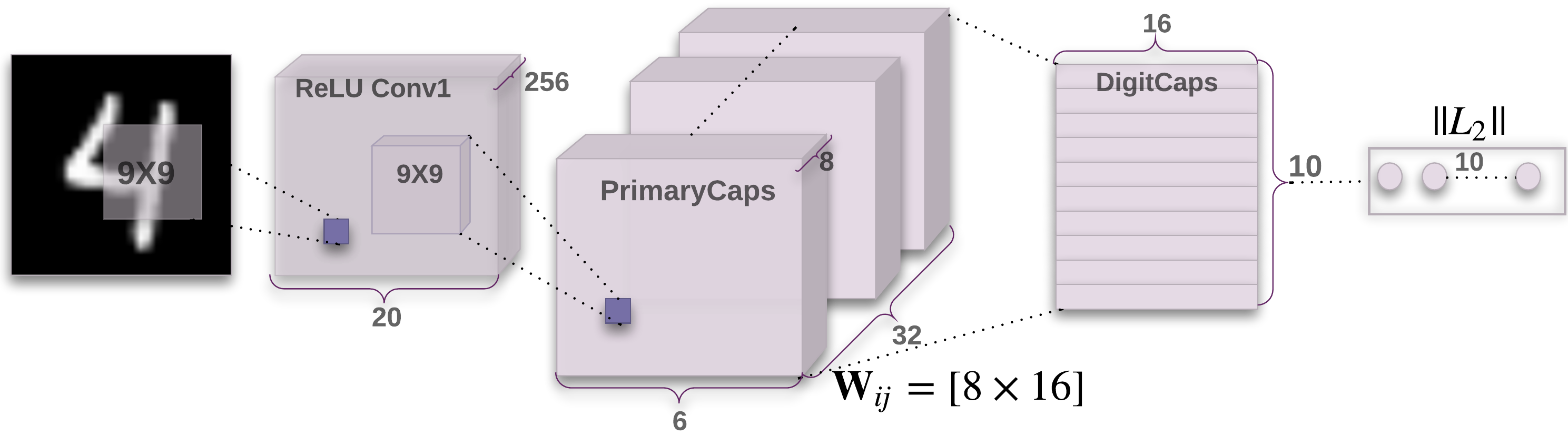
一个简单的 CapsNet 架构如图1所示。 该架构很浅，只有两个卷积层和一个全连接层。 Conv$1$ 具有 $256$、$9\times 9$ 卷积核，步幅为 1，并具有 ReLU 激活。 该层将像素强度转换为局部特征检测器的活动，然后用作主胶囊的输入。

主胶囊是多维实体的最低级别，从逆图形的角度来看，激活主胶囊对应于反转渲染过程。 这是一种非常不同的计算类型，与将实例化的部分拼凑在一起形成熟悉的整体是一种非常不同的计算类型，而这正是胶囊设计所擅长的。

第二层 (PrimaryCapsules) 是一个卷积胶囊层，具有 $32$ 个卷积 $8$D 胶囊通道(即 每个主胶囊包含 8 个卷积单元，其中 $9\times 9$ 内核，步幅为 2)。 每个主胶囊输出都会看到所有感受野与胶囊中心位置重叠的 $256\times 81$ Conv$1$ 单元的输出。 PrimaryCapsules 总共有 $[32\times 6\times 6]$ 个胶囊输出（每个输出是一个 $8$D 向量），并且 $[6\times 6]$ 网格中的每个胶囊彼此共享权重。 人们可以将 PrimaryCapsules 视为具有等式 1 的卷积层。 1 作为其块非线性。 最后一层 (DigitCaps) 每个数字类别有一个 $16$D 胶囊，每个胶囊都接收来自下一层中所有胶囊的输入。

我们仅在两个连续的胶囊层（例如 PrimaryCapsules 和 DigitCaps）之间进行路由。 由于 Conv$1$ 输出为 $1$D，因此其空间中没有一致的方向。 因此，Conv$1$ 和 PrimaryCapsule 之间不使用路由。 所有路由日志 ($b_{ij}$) 都初始化为零。 因此，最初胶囊输出 (${𝐮}_i$) 以相同的概率 ($c_{ij}$) 发送到所有父胶囊 (${𝐯}_0\mathrm{\dots }{𝐯}_9$)。

我们的实现是在 TensorFlow 中实现的 (Abadi 等人 (2016))，并使用 Adam 优化器 (Kingma 和 Ba (2014)) 及其 TensorFlow 默认参数，包括指数衰减的学习率，以最小化等式中的边际损失之和。 4。

4.1 重构作为正则化方法

图2： 用于从 DigitCaps 层表示重建数字的解码器结构。 图像与 Sigmoid 层输出之间的欧氏距离在训练过程中被最小化。 我们在训练过程中使用真实标签作为重建目标。

Figure 3: Sample MNIST test reconstructions of a CapsNet with 3 routing iterations. $(l,p,r)$ represents the label, the prediction and the reconstruction target respectively. The two rightmost columns show two reconstructions of a failure example and it explains how the model confuses a $5$ and a $3$ in this image. The other columns are from correct classifications and shows that model preserves many of the details while smoothing the noise.

$(l,p,r)$	$(2,2,2)$	$(5,5,5)$	$(8,8,8)$	$(9,9,9)$	$(5,3,5)$	$(5,3,3)$
1cmInput
Output

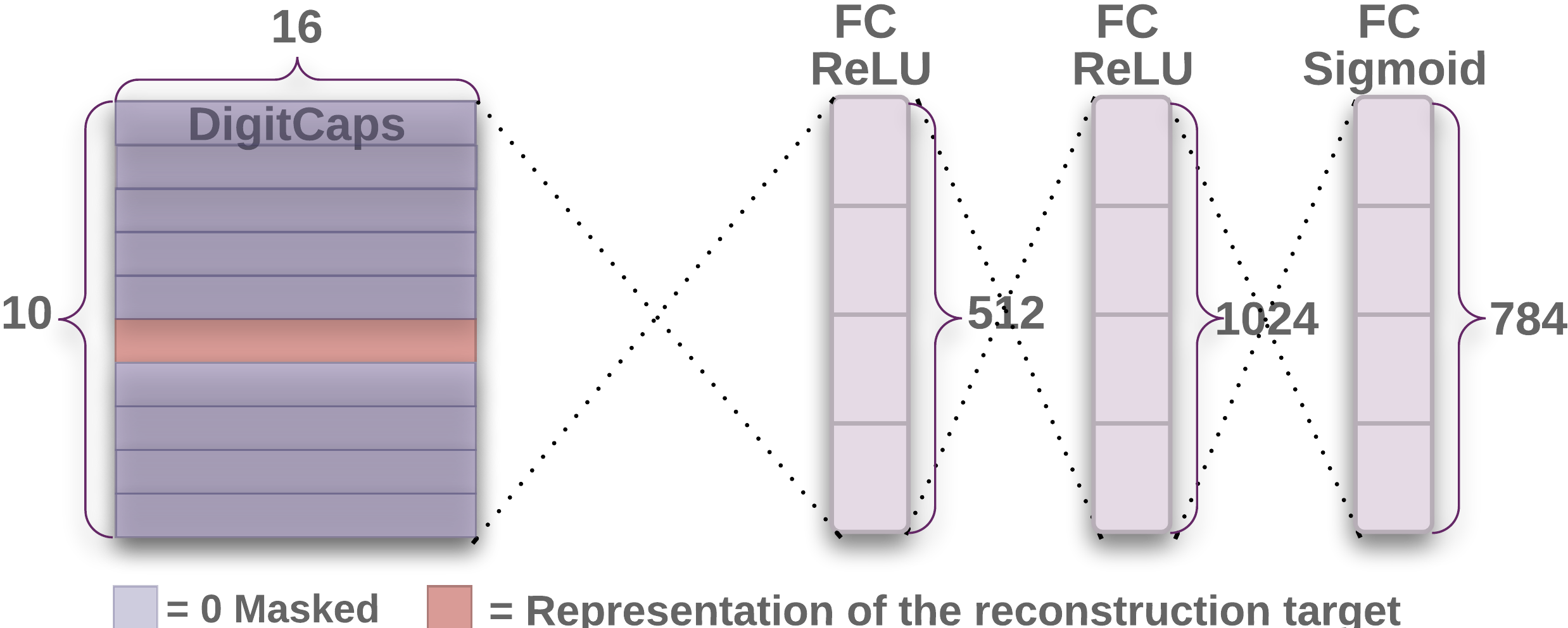
We use an additional reconstruction loss to encourage the digit capsules to encode the instantiation parameters of the input digit. During training, we mask out all but the activity vector of the correct digit capsule. Then we use this activity vector to reconstruct the input image. The output of the digit capsule is fed into a decoder consisting of $3$ fully connected layers that model the pixel intensities as described in Fig. 2. We minimize the sum of squared differences between the outputs of the logistic units and the pixel intensities. We scale down this reconstruction loss by $0.0005$ so that it does not dominate the margin loss during training. As illustrated in Fig. 3 the reconstructions from the $16$D output of the CapsNet are robust while keeping only important details.

5 Capsules on MNIST

Training is performed on $28\times 28$ MNIST (LeCun et al. (1998)) images that have been shifted by up to $2$ pixels in each direction with zero padding. No other data augmentation/deformation is used. The dataset has $60$K and $10$K images for training and testing respectively.

We test using a single model without any model averaging. Wan et al. (2013) achieves $0.21$% test error with ensembling and augmenting the data with rotation and scaling. They achieve $0.39$% without them. We get a low test error ($\mathbf{0.25}$%) on a $3$ layer network previously only achieved by deeper networks. Tab. 1 reports the test error rate on MNIST for different CapsNet setups and shows the importance of routing and reconstruction regularizer. Adding the reconstruction regularizer boosts the routing performance by enforcing the pose encoding in the capsule vector.

The baseline is a standard CNN with three convolutional layers of $256,256,128$ channels. Each has 5x5 kernels and stride of 1. The last convolutional layers are followed by two fully connected layers of size $328,192$. The last fully connected layer is connected with dropout to a $10$ class softmax layer with cross entropy loss. The baseline is also trained on 2-pixel shifted MNIST with Adam optimizer. The baseline is designed to achieve the best performance on MNIST while keeping the computation cost as close as to CapsNet. In terms of number of parameters the baseline has 35.4M while CapsNet has 8.2M parameters and 6.8M parameters without the reconstruction subnetwork.

Table 1: CapsNet classification test accuracy. The MNIST average and standard deviation results are reported from $3$ trials.

Method	Routing	Reconstruction	MNIST (%)	MultiMNIST (%)
Baseline	-	-	$0.39$	$8.1$
CapsNet	1	no	${0.34}_{\pm 0.032}$	-
CapsNet	1	yes	${0.29}_{\pm 0.011}$	$7.5$
CapsNet	3	no	${0.35}_{\pm 0.036}$	-
CapsNet	3	yes	${\mathbf{0.25}}_{\pm 0.005}$	$\mathbf{5.2}$

5.1 What the individual dimensions of a capsule represent

Figure 4: Dimension perturbations. Each row shows the reconstruction when one of the $16$ dimensions in the DigitCaps representation is tweaked by intervals of $0.05$ in the range $[-0.25,0.25]$.

Scale and thickness
Localized part
Stroke thickness
Localized skew
Width and translation
Localized part

Since we are passing the encoding of only one digit and zeroing out other digits, the dimensions of a digit capsule should learn to span the space of variations in the way digits of that class are instantiated. These variations include stroke thickness, skew and width. They also include digit-specific variations such as the length of the tail of a 2. We can see what the individual dimensions represent by making use of the decoder network. After computing the activity vector for the correct digit capsule, we can feed a perturbed version of this activity vector to the decoder network and see how the perturbation affects the reconstruction. Examples of these perturbations are shown in Fig. 4. We found that one dimension (out of $16$) of the capsule almost always represents the width of the digit. While some dimensions represent combinations of global variations, there are other dimensions that represent variation in a localized part of the digit. For example, different dimensions are used for the length of the ascender of a 6 and the size of the loop.

5.2 Robustness to Affine Transformations

Experiments show that each DigitCaps capsule learns a more robust representation for each class than a traditional convolutional network. Because there is natural variance in skew, rotation, style, etc in hand written digits, the trained CapsNet is moderately robust to small affine transformations of the training data.

To test the robustness of CapsNet to affine transformations, we trained a CapsNet and a traditional convolutional network (with MaxPooling and DropOut) on a padded and translated MNIST training set, in which each example is an MNIST digit placed randomly on a black background of $40\times 40$ pixels. We then tested this network on the affNIST data set, in which each example is an MNIST digit with a random small affine transformation. Our models were never trained with affine transformations other than translation and any natural transformation seen in the standard MNIST. An under-trained CapsNet with early stopping which achieved 99.23% accuracy on the expanded MNIST test set achieved 79% accuracy on the affnist test set. A traditional convolutional model with a similar number of parameters which achieved similar accuracy (99.22%) on the expanded mnist test set only achieved 66% on the affnist test set.

6 Segmenting highly overlapping digits

Dynamic routing can be viewed as a parallel attention mechanism that allows each capsule at one level to attend to some active capsules at the level below and to ignore others. This should allow the model to recognize multiple objects in the image even if objects overlap. Hinton et al. propose the task of segmenting and recognizing highly overlapping digits (Hinton et al. (2000) and others have tested their networks in a similar domain (Goodfellow et al. (2013), Ba et al. (2014), Greff et al. (2016)). The routing-by-agreement should make it possible to use a prior about the shape of objects to help segmentation and it should obviate the need to make higher-level segmentation decisions in the domain of pixels.

6.1 MultiMNIST dataset

Figure 5: Sample reconstructions of a CapsNet with 3 routing iterations on MultiMNIST test dataset. The two reconstructed digits are overlayed in green and red as the lower image. The upper image shows the input image. L:$(l_1,l_2)$ represents the label for the two digits in the image and R:$(r_1,r_2)$ represents the two digits used for reconstruction. The two right most columns show two examples with wrong classification reconstructed from the label and from the prediction (P). In the $(2,8)$ example the model confuses $8$ with a $7$ and in $(4,9)$ it confuses $9$ with $0$. The other columns have correct classifications and show that the model accounts for all the pixels while being able to assign one pixel to two digits in extremely difficult scenarios (column $1-4$). Note that in dataset generation the pixel values are clipped at 1. The two columns with the (*) mark show reconstructions from a digit that is neither the label nor the prediction. These columns suggests that the model is not just finding the best fit for all the digits in the image including the ones that do not exist. Therefore in case of $(5,0)$ it cannot reconstruct a $7$ because it knows that there is a $5$ and $0$ that fit best and account for all the pixels. Also, in case of $(8,1)$ the loop of $8$ has not triggered $0$ because it is already accounted for by $8$. Therefore it will not assign one pixel to two digits if one of them does not have any other support.

R:$(2,7)$	R:$(6,0)$	R:$(6,8)$	R:$(7,1)$	*R:$(5,7)$	*R:$(2,3)$	R:$(2,8)$	R:P:$(2,7)$
L:$(2,7)$	L:$(6,0)$	L:$(6,8)$	L:$(7,1)$	L:$(5,0)$	L:$(4,3)$	L:$(2,8)$	L:$(2,8)$
R:$(8,7)$	R:$(9,4)$	R:$(9,5)$	R:$(8,4)$	*R:$(0,8)$	*R:$(1,6)$	R:$(4,9)$	R:P:$(4,0)$
L:$(8,7)$	L:$(9,4)$	L:$(9,5)$	L:$(8,4)$	L:$(1,8)$	L:$(7,6)$	L:$(4,9)$	L:$(4,9)$

We generate the MultiMNIST training and test dataset by overlaying a digit on top of another digit from the same set (training or test) but different class. Each digit is shifted up to $4$ pixels in each direction resulting in a $36\times 36$ image. Considering a digit in a $28\times 28$ image is bounded in a $20\times 20$ box, two digits bounding boxes on average have $80$% overlap. For each digit in the MNIST dataset we generate $1$K MultiMNIST examples. So the training set size is $60$M and the test set size is $10$M.

6.2 MultiMNIST results

Our $3$ layer CapsNet model trained from scratch on MultiMNIST training data achieves higher test classification accuracy than our baseline convolutional model. We are achieving the same classification error rate of $5.0$% on highly overlapping digit pairs as the sequential attention model of Ba et al. (2014) achieves on a much easier task that has far less overlap ($80$% overlap of the boxes around the two digits in our case vs % for Ba et al. (2014)). On test images, which are composed of pairs of images from the test set, we treat the two most active digit capsules as the classification produced by the capsules network. During reconstruction we pick one digit at a time and use the activity vector of the chosen digit capsule to reconstruct the image of the chosen digit (we know this image because we used it to generate the composite image). The only difference with our MNIST model is that we increased the period of the decay step for the learning rate to be $10\times$ larger because the training dataset is larger.

The reconstructions illustrated in Fig. 5 show that CapsNet is able to segment the image into the two original digits. Since this segmentation is not at pixel level we observe that the model is able to deal correctly with the overlaps (a pixel is on in both digits) while accounting for all the pixels. The position and the style of each digit is encoded in DigitCaps. The decoder has learned to reconstruct a digit given the encoding. The fact that it is able to reconstruct digits regardless of the overlap shows that each digit capsule can pick up the style and position from the votes it is receiving from PrimaryCapsules layer.

Tab. 1 emphasizes the importance of capsules with routing on this task. As a baseline for the classification of CapsNet accuracy we trained a convolution network with two convolution layers and two fully connected layers on top of them. The first layer has $512$ convolution kernels of size $9\times 9$ and stride $1$. The second layer has $256$ kernels of size $5\times 5$ and stride $1$. After each convolution layer the model has a pooling layer of size $2\times 2$ and stride $2$. The third layer is a $1024$D fully connected layer. All three layers have ReLU non-linearities. The final layer of $10$ units is fully connected. We use the TensorFlow default Adam optimizer (Kingma and Ba (2014)) to train a sigmoid cross entropy loss on the output of final layer. This model has $24.56$M parameters which is $2$ times more parameters than CapsNet with $11.36$M parameters. We started with a smaller CNN ($32$ and $64$ convolutional kernels of $5\times 5$ and stride of $1$ and a $512$D fully connected layer) and incrementally increased the width of the network until we reached the best test accuracy on a $10$K subset of the MultiMNIST data. We also searched for the right decay step on the $10$K validation set.

We decode the two most active DigitCaps capsules one at a time and get two images. Then by assigning any pixel with non-zero intensity to each digit we get the segmentation results for each digit.

7 Other datasets

We tested our capsule model on CIFAR10 and achieved 10.6% error with an ensemble of 7 models each of which is trained with $3$ routing iterations on $24\times 24$ patches of the image. Each model has the same architecture as the simple model we used for MNIST except that there are three color channels and we used $64$ different types of primary capsule. We also found that it helped to introduce a "none-of-the-above" category for the routing softmaxes, since we do not expect the final layer of ten capsules to explain everything in the image. 10.6% test error is about what standard convolutional nets achieved when they were first applied to CIFAR10 (Zeiler and Fergus (2013)).

One drawback of Capsules which it shares with generative models is that it likes to account for everything in the image so it does better when it can model the clutter than when it just uses an additional “orphan” category in the dynamic routing. In CIFAR-10, the backgrounds are much too varied to model in a reasonable sized net which helps to account for the poorer performance.

We also tested the exact same architecture as we used for MNIST on smallNORB (LeCun et al. (2004)) and achieved $2.7\%$ test error rate, which is on-par with the state-of-the-art (Cireşan et al. (2011)). The smallNORB dataset consists of 96x96 stereo grey-scale images. We resized the images to 48x48 and during training processed random 32x32 crops of them. We passed the central 32x32 patch during test.

We also trained a smaller network on the small training set of SVHN (Netzer et al. (2011)) with only 73257 images. We reduced the number of first convolutional layer channels to 64, the primary capsule layer to 16 $6D$-capsules with $8D$ final capsule layer at the end and achieved $4.3\%$ on the test set.

8 Discussion and previous work

For thirty years, the state-of-the-art in speech recognition used hidden Markov models with Gaussian mixtures as output distributions. These models were easy to learn on small computers, but they had a representational limitation that was ultimately fatal: The one-of-n representations they use are exponentially inefficient compared with, say, a recurrent neural network that uses distributed representations. To double the amount of information that an HMM can remember about the string it has generated so far, we need to square the number of hidden nodes. For a recurrent net we only need to double the number of hidden neurons.

Now that convolutional neural networks have become the dominant approach to object recognition, it makes sense to ask whether there are any exponential inefficiencies that may lead to their demise. A good candidate is the difficulty that convolutional nets have in generalizing to novel viewpoints. The ability to deal with translation is built in, but for the other dimensions of an affine transformation we have to chose between replicating feature detectors on a grid that grows exponentially with the number of dimensions, or increasing the size of the labelled training set in a similarly exponential way. Capsules (Hinton et al. (2011)) avoid these exponential inefficiencies by converting pixel intensities into vectors of instantiation parameters of recognized fragments and then applying transformation matrices to the fragments to predict the instantiation parameters of larger fragments. Transformation matrices that learn to encode the intrinsic spatial relationship between a part and a whole constitute viewpoint invariant knowledge that automatically generalizes to novel viewpoints. Hinton et al. (2011) proposed transforming autoencoders to generate the instantiation parameters of the PrimaryCapsule layer and their system required transformation matrices to be supplied externally. We propose a complete system that also answers "how larger and more complex visual entities can be recognized by using agreements of the poses predicted by active, lower-level capsules".

Capsules make a very strong representational assumption: At each location in the image, there is at most one instance of the type of entity that a capsule represents. This assumption, which was motivated by the perceptual phenomenon called "crowding" (Pelli et al. (2004)), eliminates the binding problem (Hinton (1981a)) and allows a capsule to use a distributed representation (its activity vector) to encode the instantiation parameters of the entity of that type at a given location. This distributed representation is exponentially more efficient than encoding the instantiation parameters by activating a point on a high-dimensional grid and with the right distributed representation, capsules can then take full advantage of the fact that spatial relationships can be modelled by matrix multiplies.

Capsules use neural activities that vary as viewpoint varies rather than trying to eliminate viewpoint variation from the activities. This gives them an advantage over "normalization" methods like spatial transformer networks (Jaderberg et al. (2015)): They can deal with multiple different affine transformations of different objects or object parts at the same time.

Capsules are also very good for dealing with segmentation, which is another of the toughest problems in vision, because the vector of instantiation parameters allows them to use routing-by-agreement, as we have demonstrated in this paper. The importance of dynamic routing procedure is also backed by biologically plausible models of invarient pattern recognition in the visual cortex. Hinton (1981b) proposes dynamic connections and canonical object based frames of reference to generate shape descriptions that can be used for object recognition. Olshausen et al. (1993) improves upon Hinton (1981b) dynamic connections and presents a biologically plausible, position and scale invariant model of object representations.

Research on capsules is now at a similar stage to research on recurrent neural networks for speech recognition at the beginning of this century. There are fundamental representational reasons for believing that it is a better approach but it probably requires a lot more small insights before it can out-perform a highly developed technology. The fact that a simple capsules system already gives unparalleled performance at segmenting overlapping digits is an early indication that capsules are a direction worth exploring.

Acknowledgement. Of the many who provided us with constructive comments, we are specially grateful to Robert Gens, Eric Langlois, Vincent Vanhoucke, Chris Williams, and the reviewers for their fruitful comments and corrections.

Appendix A How many routing iterations to use?

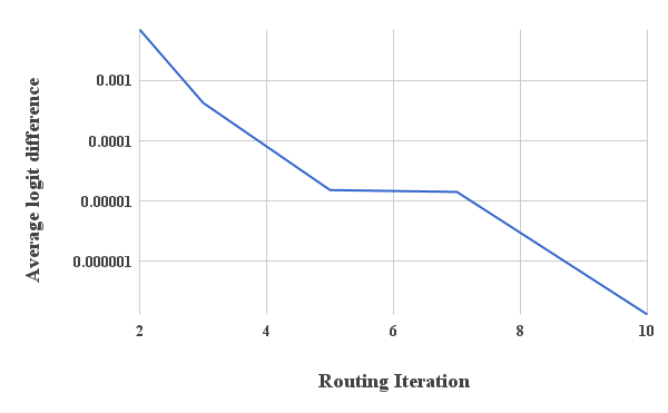
In order to experimentally verify the convergence of the routing algorithm we plot the average change in the routing logits at each routing iteration. Fig. A.1 shows the average $b_{ij}$ change after each routing iteration. Experimentally we observe that there is negligible change in the routing by $5$ iteration from the start of training. Average change in the $2^{nd}$ pass of the routing settles down after 500 epochs of training to 0.007 while at routing iteration 5 the logits only change by $1e-5$ on average.

Figure A.1: Average change of each routing logit ($b_{ij}$) by each routing iteration. After 500 epochs of training on MNIST the average change is stabilized and as it shown in right figure it decreases almost linearly in log scale with more routing iterations.

(a) During training.

(b) Log scale of final differences.

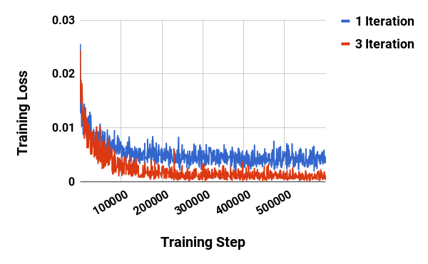
We observed that in general more routing iterations increases the network capacity and tends to overfit to the training dataset. Fig. A.2 shows a comparison of Capsule training loss on Cifar10 when trained with 1 iteration of routing vs $3$ iteration of routing. Motivated by Fig. A.2 and Fig. A.1 we suggest 3 iteration of routing for all experiments.

Figure A.2: Traning loss of CapsuleNet on cifar10 dataset. The batch size at each training step is 128. The CapsuleNet with 3 iteration of routing optimizes the loss faster and converges to a lower loss at the end.

References

- Abadi et al. [2016] Martín Abadi, Ashish Agarwal, Paul Barham, Eugene Brevdo, Zhifeng Chen, Craig Citro, Greg S Corrado, Andy Davis, Jeffrey Dean, Matthieu Devin, et al. Tensorflow: Large-scale machine learning on heterogeneous distributed systems. arXiv preprint arXiv:1603.04467, 2016.
- Ba et al. [2014] Jimmy Ba, Volodymyr Mnih, and Koray Kavukcuoglu. Multiple object recognition with visual attention. arXiv preprint arXiv:1412.7755, 2014.
- Chang and Chen [2015] Jia-Ren Chang and Yong-Sheng Chen. Batch-normalized maxout network in network. arXiv preprint arXiv:1511.02583, 2015.
- Cireşan et al. [2011] Dan C Cireşan, Ueli Meier, Jonathan Masci, Luca M Gambardella, and Jürgen Schmidhuber. High-performance neural networks for visual object classification. arXiv preprint arXiv:1102.0183, 2011.
- Goodfellow et al. [2013] Ian J Goodfellow, Yaroslav Bulatov, Julian Ibarz, Sacha Arnoud, and Vinay Shet. Multi-digit number recognition from street view imagery using deep convolutional neural networks. arXiv preprint arXiv:1312.6082, 2013.
- Greff et al. [2016] Klaus Greff, Antti Rasmus, Mathias Berglund, Tele Hao, Harri Valpola, and Jürgen Schmidhuber. Tagger: Deep unsupervised perceptual grouping. In Advances in Neural Information Processing Systems, pages 4484–4492, 2016.
- Hinton [1981a] Geoffrey E Hinton. Shape representation in parallel systems. In International Joint Conference on Artificial Intelligence Vol 2, 1981a.
- Hinton [1981b] Geoffrey E Hinton. A parallel computation that assigns canonical object-based frames of reference. In Proceedings of the 7th international joint conference on Artificial intelligence-Volume 2, pages 683–685. Morgan Kaufmann Publishers Inc., 1981b.
- Hinton et al. [2000] Geoffrey E Hinton, Zoubin Ghahramani, and Yee Whye Teh. Learning to parse images. In Advances in neural information processing systems, pages 463–469, 2000.
- Hinton et al. [2011] Geoffrey E Hinton, Alex Krizhevsky, and Sida D Wang. Transforming auto-encoders. In International Conference on Artificial Neural Networks, pages 44–51. Springer, 2011.
- Jaderberg et al. [2015] Max Jaderberg, Karen Simonyan, Andrew Zisserman, and Koray Kavukcuoglu. Spatial transformer networks. In Advances in Neural Information Processing Systems, pages 2017–2025, 2015.
- Kingma and Ba [2014] Diederik Kingma and Jimmy Ba. Adam: A method for stochastic optimization. arXiv preprint arXiv:1412.6980, 2014.
- LeCun et al. [1998] Yann LeCun, Corinna Cortes, and Christopher JC Burges. The mnist database of handwritten digits, 1998.
- LeCun et al. [2004] Yann LeCun, Fu Jie Huang, and Leon Bottou. Learning methods for generic object recognition with invariance to pose and lighting. In Computer Vision and Pattern Recognition, 2004. CVPR 2004. Proceedings of the 2004 IEEE Computer Society Conference on, volume 2, pages II–104. IEEE, 2004.
- Netzer et al. [2011] Yuval Netzer, Tao Wang, Adam Coates, Alessandro Bissacco, Bo Wu, and Andrew Y Ng. Reading digits in natural images with unsupervised feature learning. In NIPS workshop on deep learning and unsupervised feature learning, volume 2011, page 5, 2011.
- Olshausen et al. [1993] Bruno A Olshausen, Charles H Anderson, and David C Van Essen. A neurobiological model of visual attention and invariant pattern recognition based on dynamic routing of information. Journal of Neuroscience, 13(11):4700–4719, 1993.
- Pelli et al. [2004] Denis G Pelli, Melanie Palomares, and Najib J Majaj. Crowding is unlike ordinary masking: Distinguishing feature integration from detection. Journal of vision, 4(12):12–12, 2004.
- Wan et al. [2013] Li Wan, Matthew D Zeiler, Sixin Zhang, Yann LeCun, and Rob Fergus. Regularization of neural networks using dropconnect. In Proceedings of the 30th International Conference on Machine Learning (ICML-13), pages 1058–1066, 2013.
- Zeiler and Fergus [2013] Matthew D Zeiler and Rob Fergus. Stochastic pooling for regularization of deep convolutional neural networks. arXiv preprint arXiv:1301.3557, 2013.