级联扩散模型

用于高保真图像生成

摘要

我们展示了级联扩散模型能够在类条件 ImageNet 生成基准上生成高保真图像，而无需辅助图像分类器来提高样本质量。 级联扩散模型包含多个扩散模型的管道，这些模型生成分辨率不断提高的图像，从最低分辨率的标准扩散模型开始，然后是一系列或多个超分辨率扩散模型，它们依次对图像进行上采样并添加更高分辨率的细节。 我们发现，级联管道的样本质量主要取决于条件增强，这是我们提出的对超分辨率模型的低分辨率条件输入进行数据增强的方案。 我们的实验表明，条件增强可以防止级联模型在采样过程中出现累积误差，这有助于我们训练级联管道，在 64$\times$64 分辨率下实现 1.48 的 FID 分数，在 128$\times$128 分辨率下实现 3.52 的 FID 分数，在 256$\times$256 分辨率下实现 4.88 的 FID 分数，优于 BigGAN-deep，以及在 256$\times$256 分辨率下实现 63.02%（top-1）和 84.06%（top-5）的分类精度分数，优于 VQ-VAE-2。

关键词：生成模型，扩散模型，分数匹配，迭代细化，超分辨率

图 1： 包含一个基础模型和两个超分辨率模型的级联扩散模型。

1 介绍

图 2: 选定的合成 256$\times$256 ImageNet 样本。

扩散模型 (Sohl-Dickstein 等人，2015) 近年来已被证明能够合成高质量的图像和音频 (Chen 等人，2021；Ho 等人，2020；Kong 等人，2021；Song 和 Ermon，2020)：机器学习中的一个应用，长期以来一直被其他类型的生成模型所主导，例如自回归模型、GAN、VAE 和流 (Brock 等人，2019；Dinh 等人，2017；Goodfellow 等人，2014；Ho 等人，2019；Kingma 和 Dhariwal，2018；Kingma 和 Welling，2014；Razavi 等人，2019；van den Oord 等人，2016a、b、2017)。 之前关于扩散模型的大多数工作都集中在中等大小的数据集上，或者具有强条件信号的数据集上。 我们的目标是提高扩散模型在没有强条件信息可用的大型高保真数据集上的样本质量。 为了展示原始扩散形式的能力，我们专注于简单直接的技术来提高扩散模型的样本质量；例如，我们避免使用额外的图像分类器来提高样本质量指标 (Dhariwal and Nichol, 2021; Razavi et al., 2019)。

我们的主要贡献是使用 级联 来提高扩散模型在类条件 ImageNet 上的样本质量。 这里，级联指的是一种简单技术，通过学习多个分辨率下独立训练的模型管道来建模高分辨率数据；基础模型生成低分辨率样本，然后是超分辨率模型，这些模型将低分辨率样本上采样为高分辨率样本。 从级联管道进行采样是按顺序进行的，首先从低分辨率基础模型进行采样，然后从超分辨率模型进行采样，按分辨率递增的顺序进行。 虽然任何类型的生成模型都可以用于级联管道 (例如，Menick and Kalchbrenner, 2019; Razavi et al., 2019)，但在这里我们仅限于扩散模型。 最近的先前工作表明，级联可以提高扩散模型的样本质量 (Saharia et al., 2021; Nichol and Dhariwal, 2021)；我们这里的工作涉及改进扩散级联管道，以获得最佳的样本质量。

我们发现，提高级联扩散管道最简单最有效的方法是将强大的数据增强应用于每个超分辨率模型的条件输入。 我们将此技术称为 条件增强。 在我们的实验中，条件增强对于我们的级联管道在最高分辨率下生成高质量样本至关重要。 通过这种方法，我们在类条件 ImageNet 生成上的 FID 得分优于 BigGAN-Deep (Brock et al., 2019) 在任何截断值下，以及分类准确率得分优于 VQ-VAE-2 (Razavi et al., 2019)。 我们通过实证发现，条件增强之所以有效，是因为它缓解了级联管道中由于训练测试不匹配而造成的累积误差，在序列建模文献中有时被称为暴露偏差 (Bengio et al., 2015; Ranzato et al., 2016)。

本文的关键贡献如下：

• 我们表明，我们的 C级联 Diffusion Models (CDM) 生成的高保真样本优于 BigGAN-deep (Brock et al., 2019) 和 VQ-VAE-2 (Razavi et al., 2019)，在 FID 得分 (Heusel et al., 2017) 和分类准确率得分 (Ravuri and Vinyals, 2019) 方面，后者优势很大。 我们使用纯生成模型来实现这些结果，这些模型没有与任何分类器结合。

• 我们为我们的超分辨率模型引入了条件增强，并发现它对于实现高样本保真度至关重要。 我们对增强策略进行了深入探索，发现高斯增强是低分辨率上采样的关键成分，而高斯模糊是高分辨率上采样的关键成分。 我们还展示了如何有效地训练模型，这些模型在不同程度的条件增强上进行摊销，以实现训练后超参数搜索，从而获得最佳样本质量。

部分 2回顾了扩散模型的最新工作。 部分 3描述了我们发现的用于类条件ImageNet生成的最有效的条件增强类型。 部分 4包含我们的样本质量结果、消融以及对其他数据集的实验。 Section A 包含额外示例，Section B包含有关超参数和架构的详细信息。 高分辨率图像和额外的补充材料可以在 https://cascaded-diffusion.github.io/ 找到。

2 背景

我们首先介绍扩散模型、它们向条件生成扩展以及它们相关的 神经网络 架构。

2.1 扩散模型

扩散模型 (Sohl-Dickstein 等人，2015；Ho 等人，2020) 由一个正向过程定义，该过程在 $T$ 个时间步长的过程中逐渐破坏数据 ${𝐱}_0\sim q({𝐱}_0)$

$q({𝐱}_{1:T}|{𝐱}_0)$ $={\displaystyle \prod _{t=1}^T}q({𝐱}_t|{𝐱}_{t-1}),q({𝐱}_t|{𝐱}_{t-1})=𝒩({𝐱}_t;\sqrt{1-{\beta }_t}{𝐱}_{t-1},{\beta }_t𝐈)$

以及一个参数化的反向过程 $p_{\theta }({𝐱}_0)=\int p_{\theta }({𝐱}_{0:T})𝑑{𝐱}_{1:T}$，其中

$p_{\theta }({𝐱}_{0:T})$ $=p({𝐱}_T){\displaystyle \prod _{t=1}^T}{p}_{\theta }({𝐱}_{t-1}|{𝐱}_t),p_{\theta }({𝐱}_{t-1}|{𝐱}_t)=𝒩({𝐱}_{t-1};{𝝁}_{\theta }({𝐱}_t,t),{𝚺}_{\theta }({𝐱}_t,t)).$

正向过程超参数 ${\beta }_t$ 被设置为使 ${𝐱}_T$ تقریباً 分布于标准正态分布，因此 $p({𝐱}_T)$ 也被设置为标准正态先验。 反向过程被训练以通过优化证据下界 (ELBO) $-L_{\theta }({𝐱}_0)\le \log p_{\theta }({𝐱}_0)$ 来匹配正向过程的联合分布：

$L_{\theta }({𝐱}_0)$ $={𝔼}_q[L_T({𝐱}_0)+{\displaystyle \sum _{t>1}}{D}_{\mathrm{KL}}(q({𝐱}_{t-1}|{𝐱}_t,{𝐱}_0)\parallel p_{\theta }({𝐱}_{t-1}|{𝐱}_t))-\log p_{\theta }({𝐱}_0|{𝐱}_1)]$ (1)

其中 $L_T({𝐱}_0)=D_{\mathrm{KL}}\left(q({𝐱}_T|{𝐱}_0)\parallel p({𝐱}_T)\right)$。 正向过程后验 $q({𝐱}_{t-1}|{𝐱}_t,{𝐱}_0)$ 和边际 $q({𝐱}_t|{𝐱}_0)$ 为高斯分布，ELBO 中的 KL 散度可以在封闭形式中计算。 因此，可以通过对 等式 1 的随机项进行随机梯度步长来训练扩散模型。 如前所述 (Ho 等人，2020；Nichol 和 Dhariwal，2021)，我们使用反向过程参数化

${𝝁}_{\theta }({𝐱}_t,t)$ $=$ ${\displaystyle \frac{1}{\sqrt{{\alpha }_t}}}\left({𝐱}_t-{\displaystyle \frac{{\beta }_t}{\sqrt{1-{\overline{\alpha }}_t}}}{\mathit{ϵ}}_{\theta }({𝐱}_t,t)\right)$

${\mathrm{\Sigma }}_{\theta }^{ii}({𝐱}_t,t)$ $=$ $\exp (\log {\tilde{\beta }}_t+(\log {\beta }_t-\log {\tilde{\beta }}_t)v_{\theta }^i({𝐱}_t,t))$

其中 ${\alpha }_t=1-{\beta }_t$，${\overline{\alpha }}_t={\prod }_{s=1}^t{\alpha }_s$ 和 ${\tilde{\beta }}_t=\frac{1-{\overline{\alpha }}_{t-1}}{1-{\overline{\alpha }}_t}{\beta }_t$。

通过优化修改后的损失而不是 ELBO，可以提高样本质量，但会以对数似然的代价为代价。 修改后的损失的具体形式取决于我们是在学习 ${𝚺}_{\theta }$ 还是将其视为固定超参数（以及是否 ${𝚺}_{\theta }$ 是学习的，本身被认为是我们通过实验设置的超参数选择）。 对于非学习的 ${𝚺}_{\theta }$ 的情况，我们使用简化的损失

$L_{\mathrm{simple}}(\theta )={𝔼}_{{𝐱}_0,\mathit{ϵ}\sim 𝒩(\mathrm{𝟎},𝐈),t\sim 𝒰(\{1,\mathrm{\dots },T\})}\left[{\Vert {\mathit{ϵ}}_{\theta }(\sqrt{{\overline{\alpha }}_t}{𝐱}_0+\sqrt{1-{\overline{\alpha }}_t}\mathit{ϵ},t)-\mathit{ϵ}\Vert }^2\right]$

这是一种加权形式的 ELBO，类似于跨多个噪声尺度进行去噪分数匹配 (Ho 等人，2020；Song 和 Ermon，2019)。 对于学习的 ${𝚺}_{\theta }$ 的情况，我们采用混合损失 (Nichol 和 Dhariwal，2021)，使用表达式实现

$L_{\mathrm{hybrid}}(\theta )=L_{\mathrm{simple}}(\theta )+\lambda L_{\mathrm{vb}}(\theta )$

其中 $L_{\mathrm{vb}}={𝔼}_{{𝐱}_0}\left[L_{\theta }({𝐱}_0)\right]$ 并且对 $L_{\theta }$ 内部的 ${\mathit{ϵ}}_{\theta }$ 项应用停止梯度。 优化这种混合损失具有同时使用 $L_{\mathrm{simple}}$ 学习 ${𝝁}_{\theta }$ 和使用 ELBO 学习 ${𝚺}_{\theta }$ 的效果。

2.2 条件扩散模型

在条件生成设置中，数据 ${𝐱}_0$ 具有关联的条件信号 $𝐜$，例如在类条件生成的情况下为标签，或在超分辨率的情况下为低分辨率图像 (Saharia 等人，2021；Nichol 和 Dhariwal，2021)。 然后目标是学习条件模型 $p_{\theta }({𝐱}_0|𝐜)$。 为此，我们修改扩散模型以包含 $𝐜$ 作为反向过程的输入：

$p_{\theta }({𝐱}_{0:T}|𝐜)$ $=p({𝐱}_T){\displaystyle \prod _{t=1}^T}{p}_{\theta }({𝐱}_{t-1}|{𝐱}_t,𝐜),p_{\theta }({𝐱}_{t-1}|{𝐱}_t,𝐜)=𝒩({𝐱}_{t-1};{𝝁}_{\theta }({𝐱}_t,t,𝐜),{𝚺}_{\theta }({𝐱}_t,t,𝐜))$

$L_{\theta }({𝐱}_0|𝐜)$ $={𝔼}_q[L_T({𝐱}_0)+{\displaystyle \sum _{t>1}}{D}_{\mathrm{KL}}(q({𝐱}_{t-1}|{𝐱}_t,{𝐱}_0)\parallel p_{\theta }({𝐱}_{t-1}|{𝐱}_t,𝐜))-\log p_{\theta }({𝐱}_0|{𝐱}_1,𝐜)].$

数据和条件信号 $({𝐱}_0,𝐜)$ 从数据分布中联合采样，现在称为 $q({𝐱}_0,𝐜)$，并且正向过程 $q({𝐱}_{1:T}|{𝐱}_0)$ 保持不变。 唯一需要修改的是将 $𝐜$ 作为额外输入注入神经网络函数逼近器：而不是 ${𝝁}_{\theta }({𝐱}_t,t)$，我们现在有 ${𝝁}_{\theta }({𝐱}_t,t,𝐜)$，同样对于 ${𝚺}_{\theta }$。 将这些额外输入注入的具体架构选择取决于条件 $𝐜$ 的类型，如下所述。

2.3 架构

目前图像扩散模型最佳的架构是 U-Net (Ronneberger 等人，2015; Salimans 等人，2017)，它是一种将损坏的数据 ${𝐱}_t$ 映射到与 ${𝐱}_t$ 具有相同空间维度的反向过程参数 $({𝝁}_{\theta },{𝚺}_{\theta })$ 的自然选择。 标量条件，例如类别标签或扩散时间步长 $t$，是通过将嵌入添加到网络的中间层来提供的 (Ho 等人，2020)。 低分辨率图像条件是通过将低分辨率图像（通过双线性或双三次上采样处理到所需分辨率）与反向过程输入 ${𝐱}_t$ 进行通道级联来提供的，如 SR3 (Saharia 等人，2021) 和改进的 DDPM (Nichol 和 Dhariwal，2021) 模型中所述。 请参见 图 3 以了解我们在本文中使用的基于 SR3 的架构的说明。

、$M_2$

图 3： CDM 管道中每个模型使用的 U-Net 架构。 第一个模型是类别条件扩散模型，它接收噪声图像 ${𝐱}_t$ 和类别标签 $y$ 作为输入。 （类别标签 $y$ 和时间步长 $t$ 作为嵌入注入到每个块中，此处未显示）。 管道中剩余的模型是类别条件超分辨率模型，它们接收 ${𝐱}_t$、$y$ 和一个额外的上采样低分辨率图像 $𝐳$ 作为输入。 下采样/上采样块通过每个 $K$ 块将图像输入分辨率 $N\times N$ 调整 2 倍。 每个块的通道数使用通道乘数 $M_1$、$M_2$、…、$M_K$ 指定，上采样过程具有与下采样过程的级联跳跃连接。

3 级联扩散模型中的条件增强

假设 ${𝐱}_0$ 是高分辨率数据，而 ${𝐳}_0$ 是其低分辨率对应数据。 我们使用术语 级联管道 来指代一系列生成模型。 在低分辨率下，我们有一个扩散模型 $p_{\theta }({𝐳}_0)$，而在高分辨率下，则有一个超分辨率扩散模型 $p_{\theta }({𝐱}_0|{𝐳}_0)$。 级联管道形成了一个针对高分辨率数据的潜在变量模型；即 $p_{\theta }({𝐱}_0)=\int p_{\theta }({𝐱}_0|{𝐳}_0)p_{\theta }({𝐳}_0)𝑑{𝐳}_0$。 将此扩展到超过两个分辨率是直观的。 同样直观的是将整个级联管道根据类信息或其他条件信息进行条件化 $𝐜$：模型采用 $p_{\theta }({𝐳}_0|𝐜)$ 和 $p_{\theta }({𝐱}_0|{𝐳}_0,𝐜)$ 的形式，每个模型都使用 第 2.2 节中描述的条件机制。 图4中描述了一个示例级联管道。

图 4： 生成类条件 256$\times$256 图像的详细 CDM 管道。 第一个模型是类条件扩散模型，后面跟着两个类条件超分辨率扩散模型序列。 每个模型都有一个 U-Net 架构，如图图3所示。

级联管道已被证明对其他生成模型族很有用 (Menick 和 Kalchbrenner，2019；Razavi 等人，2019)。 与在最高分辨率下训练标准模型相比，训练级联管道的一个主要好处是，大部分建模能力可以专门用于低分辨率，这在经验上对样本质量至关重要，并且在低分辨率下训练和采样往往是最具计算效率的。 此外，级联允许单独训练各个模型，并且可以在每个特定分辨率上调整架构选择，以获得整个管道的最佳性能。

我们发现，提高级联管道样本质量的最有效技术是使用数据增强来训练每个超分辨率模型，方法是在其低分辨率输入上进行数据增强。 我们将这种通用技术称为 条件增强。 从高层次上讲，对于从低分辨率图像 $𝐳$ 到高分辨率图像 ${𝐱}_0$ 的某个超分辨率模型 $p_{\theta }({𝐱}_0|𝐳)$，条件增强是指对 $𝐳$ 应用某种形式的数据增强。 此增强可以采取任何形式，但我们发现在低分辨率下最有效的是添加高斯噪声（前向过程噪声），而在高分辨率下，则是对 $𝐳$ 随机应用高斯模糊。 在某些情况下，我们发现对条件增强强度进行摊销来训练超分辨率模型更实用，并在训练后的超参数搜索中选择最佳强度，以获得最佳样本质量。 以下部分将详细介绍条件增强及其在训练和采样过程中的实现。

3.1 模糊增强

条件增强的简单实例是通过模糊来增强 $𝐳$。 我们发现这种方法在对分辨率为 128$\times$128 和 256$\times$256 的图像进行上采样时最为有效。 更具体地说，我们应用大小为 $k$、sigma 为 $\sigma$ 的高斯滤波器来获得 ${𝐳}_b$。 我们使用大小为 $k=(3,3)$ 的滤波器，并在训练期间从固定范围内随机采样 $\sigma$。 我们执行超参数搜索以找到 $\sigma$ 的范围。 在训练期间，我们将这种模糊增强应用于 50% 的示例。 在推理期间，不对低分辨率输入应用任何增强。 我们探索了在推理期间应用不同程度的模糊增强，但在初步实验中没有发现它有帮助。

3.2 截断条件增强

在这里，我们描述了我们称之为 截断条件增强 的方法，这是一种条件增强形式，它需要对超分辨率模型的训练和架构进行简单的修改，但在级联的初始阶段不需要对低分辨率模型进行任何更改。 我们发现这种方法在分辨率小于 128$\times$128 时最为有用。 通常，生成高分辨率样本 ${𝐱}_0$ 包括先从低分辨率模型 $p_{\theta }({𝐳}_0)$ 生成 ${𝐳}_0$，然后将结果馈送到超分辨率模型 $p_{\theta }({𝐱}_0|{𝐳}_0)$ 中。 换句话说，使用潜在变量模型的祖先采样来生成高分辨率样本

$p_{\theta }({𝐱}_0)={\displaystyle \int p_{\theta }({𝐱}_0|{𝐳}_0)p_{\theta }({𝐳}_0)𝑑{𝐳}_0}={\displaystyle \int p_{\theta }({𝐱}_0|{𝐳}_0)p_{\theta }({𝐳}_{0:T})𝑑{𝐳}_{0:T}}.$

(为简单起见，我们假设低分辨率模型和超分辨率模型都使用相同数量的时间步长 $T$。) 截断条件增强是指将低分辨率逆过程截断到时间步长 $s>0$，而不是 $0$；即，

$p_{\theta }^s({𝐱}_0)={\displaystyle \int p_{\theta }({𝐱}_0|{𝐳}_s)p_{\theta }({𝐳}_s)𝑑{𝐳}_s}={\displaystyle \int p_{\theta }({𝐱}_0|{𝐳}_s)p_{\theta }({𝐳}_{s:T})𝑑{𝐳}_{s:T}}.$ (2)

基模型现在是 $p_{\theta }({𝐳}_s)=\int p_{\theta }({𝐳}_{s:T})𝑑{𝐳}_{s+1:T}$，而超分辨率模型现在是 $p_{\theta }({𝐱}_0|{𝐳}_s)=\int p({𝐱}_T){\prod }_{t=1}^T{p}_{\theta }({𝐱}_{t-1}|{𝐱}_t,{𝐳}_s)d{𝐱}_{1:T}$，其中

$p_{\theta }({𝐱}_{t-1}|{𝐱}_t,{𝐳}_s)=𝒩({𝐱}_{t-1};{𝝁}_{\theta }({𝐱}_t,t,{𝐳}_s,s),{𝚺}_{\theta }({𝐱}_t,t,{𝐳}_s,s)).$

截断低分辨率逆过程是一种数据增强形式的原因是，$p_{\theta }({𝐱}_0|{𝐳}_s)$ 的训练过程涉及对有噪声的 ${𝐳}_s\sim q({𝐳}_s|{𝐳}_0)$ 进行条件化，它在比例上是 ${𝐳}_0$ 增强了高斯噪声。 为了更准确地说明使用截断条件增强训练级联管道，让我们检查 Eq. 2 中 $p_{\theta }^s({𝐱}_0)$ 的 ELBO。 我们可以将 $p_{\theta }^s({𝐱}_0)$ 视为具有扩散模型先验、扩散模型解码器和近似后验的 VAE

$q({𝐱}_{1:T},{𝐳}_{1:T}|{𝐱}_0,{𝐳}_0)={\displaystyle \prod _{t=1}^T}q({𝐱}_t|{𝐱}_{t-1})q({𝐳}_t|{𝐳}_{t-1}),$

它在低分辨率和高分辨率对上独立运行正向过程。 ELBO 为

$-\log p_{\theta }^s({𝐱}_0)\le {𝔼}_q[L_T({𝐳}_0)+{\displaystyle \sum _{t>s}}{D}_{\mathrm{KL}}(q({𝐳}_{t-1}|{𝐳}_t,{𝐳}_0)\parallel p_{\theta }({𝐳}_{t-1}|{𝐳}_t))-\log p_{\theta }({𝐱}_0|{𝐳}_s)],$

其中 $L_T({𝐳}_0)=D_{\mathrm{KL}}\left(q({𝐳}_T|{𝐳}_0)\parallel p({𝐳}_T)\right)$。 请注意，对 $t$ 的求和在 $s$ 处被截断，解码器 $p_{\theta }({𝐱}_0|{𝐳}_s)$ 是在 ${𝐳}_s$ 条件下的超分辨率模型。 解码器本身具有 $-\log p_{\theta }({𝐱}_0|{𝐳}_s)\le L_{\theta }({𝐱}_0|{𝐳}_s)$ 形式的 ELBO，其中

$L_{\theta }({𝐱}_0|{𝐳}_s)={𝔼}_q[L_T({𝐱}_0)+{\displaystyle \sum _{t>1}}{D}_{\mathrm{KL}}(q({𝐱}_{t-1}|{𝐱}_t,{𝐱}_0)\parallel p_{\theta }({𝐱}_{t-1}|{𝐱}_t,{𝐳}_s))-\log p_{\theta }({𝐱}_0|{𝐱}_1,{𝐳}_s)].$

因此，我们有组合模型的 ELBO

$-\log p_{\theta }^s({𝐱}_0)\le {𝔼}_q[L_T({𝐳}_0)+{\displaystyle \sum _{t>s}}{D}_{\mathrm{KL}}(q({𝐳}_{t-1}|{𝐳}_t,{𝐳}_0)\parallel p_{\theta }({𝐳}_{t-1}|{𝐳}_t))+L_{\theta }({𝐱}_0|{𝐳}_s)].$ (3)

很明显，优化 Eq. 3 会分别训练低分辨率模型和高分辨率模型。 对于 $s$ 的固定值，低分辨率过程被训练到截断时间步长 $s$，而超分辨率模型被训练在使用停止在时间步长 $s$ 的低分辨率正向过程破坏的条件信号上。

在实践中，由于我们的主要目标是样本质量，因此在训练具有可学习逆过程方差的模型时，我们不会直接使用这些 ELBO 表达式。 相反，我们在 Section 2 中描述的“简单”未加权损失或混合损失上进行训练，我们使用的特定损失被认为是在 Section B 中报告的超参数。

我们希望搜索多个$s$值以选择最佳样本质量。 为了使搜索更实际，我们通过在训练时对均匀随机$s$进行摊销，避免了对模型进行重新训练。 由于每个可能的截断时间对应于一个不同的超分辨率任务，因此${𝝁}_{\theta }$和${𝚺}_{\theta }$的超分辨率模型必须将${𝐳}_s$作为输入，以及$s$，这可以通过使用具有额外时间嵌入输入的单个网络来实现$s$。 我们保留了低分辨率模型训练不变，因为标准扩散训练过程已经使用随机$s$进行训练。 两阶段级联管道完整的训练过程列在算法 1中。

3.3 非截断条件增强

另一种条件增强形式，我们称之为非截断条件增强， 使用与截断条件增强相同的模型修改和训练过程（第 3.2节）。 唯一的区别在于采样时间。 在非截断条件增强中，我们不会截断低分辨率逆过程，而是始终使用完整的、非截断的低分辨率逆过程对${𝐳}_0$进行采样；然后，我们使用正向过程将${𝐳}_0$破坏为${𝐳}_s^{\prime }\sim q({𝐳}_s|{𝐳}_0)$，并将破坏的${𝐳}_s^{\prime }$输入到超分辨率模型中。

非截断条件增强相对于截断条件增强的主要优势在于搜索$s$期间的实际优势。 在截断增强的情况下，如果我们想对所有$s$并行运行超分辨率模型，我们必须存储所有$s$值的低分辨率样本${𝐳}_s$。 在非截断增强的情况下，我们只需要存储一次低分辨率样本，因为对${𝐳}_s^{\prime }\sim q({𝐳}_s|{𝐳}_0)$进行采样在计算上是廉价的。 这些采样过程列在 算法 2中。

截断和非截断条件增强应该表现相似，因为如果低分辨率模型训练得足够好，${𝐳}_s$和${𝐳}_s^{\prime }$应该具有相似的边缘分布。 事实上，在第 4.3节中，我们凭经验发现样本质量指标对于截断和非截断条件增强都是相似的。

算法 1 使用高斯条件增强训练两阶段 CDM

1: 重复 $▷$ 训练基础模型

2:      $({𝐳}_0,𝐜)\sim p(𝐳,𝐜)$ $▷$ 采样低分辨率图像和标签

3:      $t\sim 𝒰\left(\{1,\mathrm{\dots },T\}\right)$

4:      $\mathit{ϵ}\sim 𝒩(\mathrm{𝟎},𝐈)$

5:      ${𝐳}_t=\sqrt{{\overline{\alpha }}_t}{𝐳}_0+\sqrt{1-{\overline{\alpha }}_t}\mathit{ϵ}$

6:      $\theta \leftarrow \theta -\eta {\nabla }_{\theta }{\Vert {\mathit{ϵ}}_{\theta }({𝐳}_t,t,𝐜)-\mathit{ϵ}\Vert }^2$ $▷$ 简单损失（可以替换为混合损失）

7:直到 收敛

8: 重复 $▷$ 训练超分辨率模型（与基础模型并行）

9:      $({𝐱}_0,{𝐳}_0,𝐜)\sim p(𝐱,𝐳,𝐜)$ $▷$ 对低分辨率和高分辨率图像进行采样并标注

10:      $s,t\sim 𝒰\left(\{1,\mathrm{\dots },T\}\right)$

11:      ${\mathit{ϵ}}_{𝐳},{\mathit{ϵ}}_{𝐱}\sim 𝒩(\mathrm{𝟎},𝐈)$ $▷$ 注意：${\mathit{ϵ}}_{𝐳},{\mathit{ϵ}}_{𝐱}$ 和 ${𝐳}_0,{𝐱}_0$ 的形状应分别相同

12:      ${𝐳}_t=\sqrt{{\overline{\alpha }}_s}{𝐳}_0+\sqrt{1-{\overline{\alpha }}_s}{\mathit{ϵ}}_{𝐳}$ $▷$ 应用高斯条件增强

13:      ${𝐱}_t=\sqrt{{\overline{\alpha }}_t}{𝐱}_0+\sqrt{1-{\overline{\alpha }}_t}{\mathit{ϵ}}_{𝐱}$

14:      $\theta \leftarrow \theta -\eta {\nabla }_{\theta }{\Vert {\mathit{ϵ}}_{\theta }({𝐱}_t,t,{𝐳}_s,s,𝐜)-{\mathit{ϵ}}_{𝐱}\Vert }^2$

15:直到 收敛

算法 2 从具有高斯条件增强的两阶段 CDM 中采样

1:$𝐜$: 类别标签

2:$s$: 条件增强截断时间

3:${𝐳}_T\sim 𝒩(\mathrm{𝟎},𝐈)$

4:如果 使用截断条件增强 则

5:    对于   $t=T,\mathrm{\dots },s+1$   做

6:           ${𝐳}_{t-1}\sim p_{\theta }\left({𝐳}_{t-1}|{𝐳}_t,𝐜\right)$

7:    结束 对于

8:否则

9:    对于   $t=T,\mathrm{\dots },1$   做

10:           ${𝐳}_{t-1}\sim p_{\theta }\left({𝐳}_{t-1}|{𝐳}_t,𝐜\right)$

11:    结束 为了

12:      ${𝐳}_s\sim q\left({𝐳}_s|{𝐳}_0\right)$ $▷$ 覆盖先前采样到的${𝐳}_s$的值

13:结束 如果

14:${𝐱}_T\sim 𝒩(\mathrm{𝟎},𝐈)$

15:为了   $t=T,\mathrm{\dots },1$   做

16:      ${𝐱}_{t-1}\sim p_{\theta }\left({𝐱}_{t-1}|{𝐱}_t,{𝐳}_s,𝐜\right)$

17:结束 为了

18:return ${𝐱}_0$

4 Experiments

Figure 5: Classwise Synthetic 256$\times$256 ImageNet images. Each row represents a specific ImageNet class. Classes from top to bottom - Flamingo (130), White Wolf (270), Tiger (292), Monarch Butterfly (323), Zebra (340) and Dome (538).

Figure 6: Classwise Synthetic 256$\times$256 ImageNet images. Each row represents a specific ImageNet class. Classes from top to bottom - Greenhouse (580), Model T (661), Streetcar (829), Comic Book (917), Crossword Puzzle (918), Cheeseburger (933).

We designed experiments to improve the sample quality metrics of cascaded diffusion models on class-conditional ImageNet generation. Our cascading pipelines consist of class-conditional diffusion models at all resolutions, so class information is injected at all resolutions: see Fig. 4. Our final ImageNet results are described in Section 4.1.

To give insight into our cascading pipelines, we begin with improvements on a baseline non-cascaded model at the 64$\times$64 resolution (Section 4.2), then we show that cascading up to 64$\times$64 improves upon our best non-cascaded 64$\times$64 model, but only in conjunction with conditioning augmentation. We also show that truncated and non-truncated conditioning augmentation perform equally well (Section 4.3), and we study random Gaussian blur augmentation to train super-resolution models to resolutions of 128$\times$128 and 256$\times$256 (Section 4.4). Finally, we verify that conditioning augmentation is also effective on the LSUN dataset (Yu et al., 2015) and therefore is not specific to ImageNet (Section 4.5).

我们对 ImageNet 数据集 (Russakovsky 等人，2015) 进行了裁剪和调整大小，方式与 BigGAN (Brock 等人，2019) 相同。 我们使用标准实践报告了 Inception 分数，该实践生成 50k 个样本并计算 10 个拆分的平均值和标准差 (Salimans 等人，2016)。 通常，在整个实验过程中，我们根据 10k 个样本计算的 FID 分数选择模型并进行提前停止，但所有报告的 FID 分数均根据 50k 个样本计算，以与其他工作进行比较 (Heusel 等人，2017)。 我们用于模型选择和报告模型性能的 FID 分数是根据常见做法针对训练集统计数据计算的，但由于这可以被视为对性能指标的过度拟合，因此我们还报告了使用针对验证集统计数据计算的 FID 分数的模型性能。 我们还报告了分类准确率得分 (CAS) 的结果，该得分由 Ravuri 和 Vinyals (2019) 提出，因为他们发现非 GAN 模型在 FID 和 IS 上的得分可能很低，尽管它们生成了视觉上吸引人的样本，并且 FID 和 IS 与下游任务的性能不相关（有时是反相关的）。

4.1 主要级联管道结果

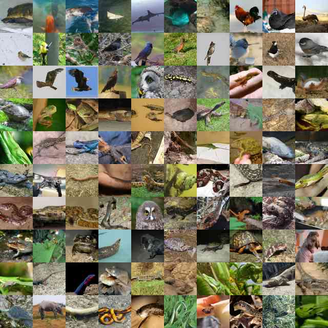
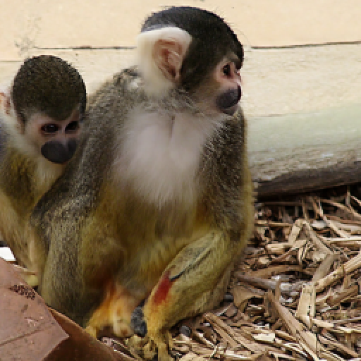
表 1(a) 报告了级联扩散模型 (CDM) 在 64$\times$64、128$\times$128 和 256$\times$256 ImageNet 数据集分辨率上的主要结果，以及基线。 CDM 在所考虑的图像分辨率上以 FID 得分优于 BigGAN-deep，但在 GAN 的截断参数针对 Inception 得分优化时，GAN 在 Inception 得分方面表现更好 (Brock 等人，2019)。 我们还优于同时发布的未使用分类器指导来提高样本质量得分的扩散模型 (Dhariwal 和 Nichol，2021)。 请参阅 图 8，以了解与 VQ-VAE-2 (Razavi 等人，2019) 和 BigGAN-deep (Brock 等人，2019) 相比的样本质量和多样性的定性评估，以及 图  5 和 6 以查看生成的图像示例。

表 1(b) 报告了 128$\times$128 和 256$\times$256 分辨率下模型在分类准确率得分 (CAS) (Ravuri 和 Vinyals，2019) 上的结果。 我们发现，CDM 在 CAS 指标上以显著优势优于 VQ-VAE-2 和 BigGAN-deep，这表明在后续任务上具有更好的潜在性能。 图 7 比较了在真实训练数据和 CDM 样本上训练的分类器的逐类分类准确率得分。 与 BigGAN-deep 和 VQ-VAE-2 分别在 6 个和 31 个类别上的表现相比，CDM 分类器在 96 个类别上优于真实数据。 我们还在附录图 11 和 12 中展示了准确率得分最高和最低的类别的样本。

我们的级联管道结构为 32$\times$32 基础模型、32$\times$32$\to$64$\times$64 超分辨率模型，随后是 64$\times$64$\to$128$\times$128 或 64$\times$64$\to$256$\times$256 超分辨率模型。 32$\times$32 和 64$\times$64 分辨率的模型使用 4000 个扩散时间步长，其架构类似于 DDPM (Ho 等人，2020) 和改进的 DDPM (Nichol 和 Dhariwal，2021)。 128$\times$128 和 256$\times$256 分辨率的模型使用 100 个采样步骤，由训练后超参数搜索确定(部分 4.4 )，并且他们使用类似于 SR3 （Saharia 等人，2021） 的架构。 所有基础分辨率和超分辨率模型都以类别标签为条件。 详情请参阅部分B。

Model	FID vs train	FID vs validation	IS
32$\times$32 resolution
CDM (ours)	1.11	1.99	26.01 $\pm$ 0.59
64$\times$64 resolution
BigGAN-deep, by (Dhariwal and Nichol, 2021)	4.06
Improved DDPM (Nichol and Dhariwal, 2021)	2.92
ADM (Dhariwal and Nichol, 2021)	2.07
CDM (ours)	1.48	2.48	67.95 $\pm$ 1.97
128$\times$128 resolution
BigGAN-deep (Brock et al., 2019)	5.7		124.5
BigGAN-deep, max IS (Brock et al., 2019)	25		253
LOGAN (Wu et al., 2019)	3.36		148.2
ADM (Dhariwal and Nichol, 2021)	5.91
CDM (ours)	3.52	3.76	128.80 $\pm$ 2.51
256$\times$256 resolution
BigGAN-deep (Brock et al., 2019)	6.9		171.4
BigGAN-deep, max IS (Brock et al., 2019)	27		317
VQ-VAE-2 (Razavi et al., 2019)	31.11
Improved DDPM (Nichol and Dhariwal, 2021)	12.26
SR3 (Saharia et al., 2021)	11.30
ADM (Dhariwal and Nichol, 2021)	10.94		100.98
ADM+upsampling (Dhariwal and Nichol, 2021)	7.49		127.49
CDM (ours)	4.88	4.63	158.71 $\pm$ 2.26

(a) 分类引导免费方法的类条件 ImageNet 样本质量结果

Model	Top-1 Accuracy	Top-5 Accuracy
128$\times$128 resolution
Real	68.82%	88.79%
BigGAN-deep (Brock et al., 2019)	40.64%	64.44%
HAM (De Fauw et al., 2019)	54.05%	77.33%
CDM (ours)	59.84%	81.79%
256$\times$256 resolution
Real	73.09%	91.47%
BigGAN-deep (Brock et al., 2019)	42.65%	65.92%
VQ-VAE-2 (Razavi et al., 2019)	54.83%	77.59%
CDM (ours)	63.02%	84.06%

(b) 分类准确率得分 (CAS) 结果

表 1： 主要结果。 只有当至少有两个可用于比较时，数字才以粗体显示。 实际数据的 CAS 和其他模型来自 Ravuri 和 Vinyals (2019)。

Figure 7: Classwise Classification Accuracy Score comparison between real data (blue) and generated data (red) at the 256$\times$256 resolution. Accompanies Table 1(b).

CDM (ours)	VQ-VAE-2	BigGAN-deep

Figure 8: Comparing the quality and diversity of model samples in selected 256$\times$256 ImageNet classes {Tench(0), Goldfish(1) and Ostrich(9)}. VQVAE-2 and BigGAN samples are taken from Razavi et al. (2019).

4.2 Baseline Model Improvements

To set a strong baseline for class-conditional ImageNet generation at the 64$\times$64 resolution, we reproduced and improved upon a 4000 timestep non-cascaded 64$\times$64 class-conditional diffusion model from Improved DDPM (Nichol and Dhariwal, 2021). Our reimplementation used dropout and was trained longer than reported by Nichol and Dhariwal; we found that adding dropout generally slowed down convergence of FID and Inception scores, but improved their best values over the course of a longer training period. We further improved the training set FID score and Inception score by adding noise to the trained model’s samples using the forward process to the 2000 timestep point, then restarting the reverse process from that point. See Table 2(a) for the resulting sample quality metrics.

4.3 Conditioning Augmentation Experiments up to 64$\times$64

Building on our reimplementation in Section 4.2, we verify in a small scale experiment that cascading improves sample quality at the 64$\times$64 resolution. We train a two-stage cascading pipeline that comprises a 16$\times$16 base model and a 16$\times$16$\to$64$\times$64 super-resolution model. The super-resolution model architecture is identical to the best 64$\times$64 non-cascaded baseline model in Section 4.2, except for the trivial modification of adding in the low resolution image conditioning information by channelwise concatenation at the input (see Section 2).

See Table 2(b) and Fig. 9 for the results of this 16$\times$16$\to$64$\times$64 cascading pipeline. Interestingly, we find that without conditioning augmentation, the cascading pipeline attains lower sample quality than the non-cascaded baseline 64$\times$64 model; the FID score, for example, degrades from 2.35 to 6.02. With sufficient conditioning augmentation, however, the sample quality of the cascading pipeline becomes better than the non-cascaded baseline. We train two super-resolution models with non-truncated conditioning augmentation, one at truncation time $s=101$ and another at $s=1001$ (we could have amortized both into a single model, but we chose not to do so in this experiment to prevent potential model capacity issues from confounding the results). The first model achieves better sample quality than the non-augmented model but is still worse than the non-cascaded baseline. The second model achieves a FID score of 2.13, outperforming the non-cascaded baseline. Conditioning augmentation is therefore crucial to improve sample quality in this particular cascading pipeline.

Model	FID vs train	FID vs validation	IS
Improved DDPM (Nichol and Dhariwal, 2021)	2.92
Our reimplementation	2.44	2.91	49.81 $\pm$ 0.65
+ more sampling steps	2.35	2.91	52.72 $\pm$ 1.15

(a) Improvements to a non-cascaded baseline

Conditioning	FID vs train	FID vs validation	IS
No cascading	2.35	2.91	52.72 $\pm$ 1.15
16$\times$16$\to$64$\times$64 cascading
$s=0$	6.02	5.84	35.59 $\pm$ 1.19
$s=101$	3.41	3.67	44.72 $\pm$ 1.12
$s=1001$	2.13	2.79	54.47 $\pm$ 1.05

(b) Small-scale ablation comparing no cascading to 16$\times$16$\to$64$\times$64 cascading

Table 2: 64$\times$64 ImageNet sample quality: ablations.

(a) 16$\times$16 base

(b) 16$\times$16$\to$64$\times$64 super-resolution, $s=0$

(c) 16$\times$16$\to$64$\times$64 super-resolution, $s=101$

(d) 16$\times$16$\to$64$\times$64 super-resolution, $s=1001$

Figure 9: Generated images for varying amounts of conditioning augmentation (non-truncated) in a small-scale 16$\times$16$\to$64$\times$64 pipeline for ablation purposes. Accompanies Table 2(b).

To further improve sample quality at the 64$\times$64 resolution, we found it helpful to increase model sizes and to switch to a cascading pipeline starting with a 32$\times$32 base resolution model. We train a 32$\times$32 base model applying random left-right flips, which we found to help 32$\times$32 scores at the expense of longer training times. Training without random flips, the best 32$\times$32 resolution FID score is 1.25 at 300k training steps, while training with random flips it is 1.11 at 700k training steps. The 32$\times$32$\to$64$\times$64 super-resolution model is now amortized over the truncation time $s$ by providing $s$ as an extra time embedding input to the network (Section 2), allowing us to perform a more fine grained search over $s$ without retraining the model.

Conditioning	FID vs train	FID vs validation	IS
No conditioning augmentation (baseline)
$s=0$	1.71	2.46	61.34 $\pm$ 1.58
Truncated conditioning augmentation
$s=251$	1.50	2.44	66.76 $\pm$ 1.76
$s=501$	1.48	2.48	67.95 $\pm$ 1.97
$s=751$	1.48	2.51	68.48 $\pm$ 1.77
$s=1001$	1.49	2.51	67.95 $\pm$ 1.51
$s=1251$	1.51	2.54	67.20 $\pm$ 1.94
$s=1501$	1.54	2.56	67.09 $\pm$ 1.67
Non-truncated conditioning augmentation
$s=251$	1.58	2.50	66.21 $\pm$ 1.51
$s=501$	1.53	2.51	67.59 $\pm$ 1.85
$s=751$	1.48	2.47	67.48 $\pm$ 1.31
$s=1001$	1.49	2.48	66.51 $\pm$ 1.59
$s=1251$	1.48	2.46	66.28 $\pm$ 1.49
$s=1501$	1.50	2.47	65.59 $\pm$ 0.86

(a) Base model for low resolution conditioning

Conditioning	FID vs train	FID vs validation	IS
Ground truth training data
$s=0$	0.76	1.76	74.84 $\pm$ 1.43
$s=251$	0.87	1.85	71.79 $\pm$ 0.89
$s=501$	0.92	1.91	70.68 $\pm$ 1.26
$s=751$	0.95	1.94	69.93 $\pm$ 1.40
$s=1001$	0.98	1.97	69.03 $\pm$ 1.26
$s=1251$	1.03	1.99	67.92 $\pm$ 1.65
$s=1501$	1.11	2.04	66.7 $\pm$ 1.21
Ground truth validation data
$s=0$	1.20	0.59	64.33 $\pm$ 1.24
$s=251$	1.27	0.96	63.17 $\pm$ 1.19
$s=501$	1.32	1.17	62.65 $\pm$ 0.76
$s=751$	1.38	1.32	62.21 $\pm$ 0.94
$s=1001$	1.42	1.44	61.53 $\pm$ 1.39
$s=1251$	1.47	1.54	60.58 $\pm$ 0.93
$s=1501$	1.53	1.64	60.02 $\pm$ 0.84

(b) Ground truth for low resolution conditioning

Table 3: 64$\times$64 ImageNet sample quality: large scale experiment comparing truncated and non-truncated conditioning augmentation for 32$\times$32$\to$64$\times$64 cascading, using amortized truncation time conditioning.

Table 3(a) displays the resulting sample quality scores for both truncated and non-truncated augmentation. The sample quality metrics improve and then degrade non-monotonically as the truncation time is increased. This indicates that moderate amounts of conditioning augmentation are beneficial to sample quality of the cascading pipeline, but too much conditioning augmentation causes the super-resolution model to behave as a non-conditioned model unable to benefit from cascading. For comparison, Table 3(b) shows sample quality when the super-resolution model is conditioned on ground truth data instead of generated data. Here, sample quality monotonically degrades as truncation time is increased. Conditioning augmentation is therefore useful precisely when conditioning on generated samples, so as a technique it is uniquely suited to cascading pipelines.

Based on these findings on non-monotonicity of sample quality with respect to truncation time, we conclude that conditioning augmentation works because it alleviates compounding error from a train-test mismatch for the super-resolution model. This occurs when low-resolution model samples are out of distribution compared to the ground truth data on which the super-resolution model is trained. A sufficient amount of Gaussian conditioning augmentation prevents the super-resolution model from attempting to upsample erroneous, out-of-distribution details in the low resolution generated samples. In contrast, sample quality degrades monotonically with respect to truncation time when conditioning the super-resolution model on ground truth data, because there is no such train-test mismatch.

Table 3(a) additionally shows that truncated and non-truncated conditioning augmentation are approximately equally effective at improving sample quality of the cascading pipeline, albeit at different values of the truncation time parameter. Thus we generally recommend non-truncated augmentation due to its practical benefits described in Section 3.3.

4.4 Experiments at 128$\times$128 and 256$\times$256

Figure 10: FID on 256$\times$256 images vs inference steps in 64$\times$64 $\to$ 256$\times$256 super-resolution.

While we found Gaussian noise augmentation to be a key ingredient to boost the performance of our cascaded models at low resolutions, our initial experiments with similar augmentations for 128$\times$128 and 256$\times$256 upsampling yielded negative results. Hence, we explore Gaussian blurring augmentation for these resolutions. As mentioned in Section 3.1, we apply the blurring augmentation 50% of the time during training, and use no blurring during inference. We explored other settings (e.g. applying blurring to all training examples, and using varying amounts of blurring during inference), but found this to be most effective in our initial experiments.

Blur $\sigma$	FID vs train	FID vs validation	IS
$\sigma =0$ (no blur)	7.26	6.42	134.53 $\pm$ 2.97
$\sigma \sim 𝒰(0.4,0.6)$	6.18	5.57	142.71 $\pm$ 2.83
$\sigma \sim 𝒰(0.4,0.8)$	6.90	6.31	136.57 $\pm$ 4.34
$\sigma \sim 𝒰(0.4,1.0)$	6.35	5.76	141.40 $\pm$ 4.34

(a) Gaussian blur noise in conditioning

Model	FID vs train	FID vs validation	IS
Baseline	6.18	5.57	142.71 $\pm$ 2.83
+ Class Conditioning	5.75	5.27	152.17 $\pm$ 2.29
+ Large Batch Training	5.00	4.71	157.84 $\pm$ 2.60
+ Flip LR	4.88	4.63	158.71 $\pm$ 2.26

(b) Further improvements on super-resolution

Table 4: 256$\times$256 ImageNet sample quality: experiments on 64$\times$64 $\to$ 256$\times$256 super-resolution.

Table 4(a) shows the results of applying Gaussian blur augmentation to the 64$\times$64 $\to$ 256$\times$256 super-resolution model. While any amount of blurring helps improve the scores of the 256$\times$256 samples over the baseline model with no blur, we found that sampling $\sigma \sim 𝒰(0.4,0.6)$ gives the best results. Table 4(b) shows further improvements from class conditioning, large batch training, and random flip augmentation for the super-resolution model. While we find class conditioning helpful for upsampling at low resolution settings, it is interesting that it still gives a huge boost to the upsampling performance at high resolutions even when the low resolution inputs at 64$\times$64 can be sufficiently informative. We also found increasing the training batch size from 256 to 1024 further improved performance by a significant margin. We also obtain marginal improvements by training the super-resolution model on randomly flipped data.

Since the sampling cost increases quadratically with the target image resolution, we attempt to minimize the number of denoising iterations for our 64$\times$64 $\to$ 256$\times$256 and 64$\times$64 $\to$ 128$\times$128 super-resolution models. To this end, we train these super-resolution models with continuous noise conditioning, like Saharia et al. (2021) and Chen et al. (2021), and tune the noise schedule for a given number of steps during inference. This tuning is relatively inexpensive as we do not need to retrain the models. We report all results using 100 inference steps for these models. Figure 10 shows FID vs number of inference steps for our 64$\times$64 $\to$ 256$\times$256 model. The FID score deteriorates marginally even when using just 4 inference steps. Interestingly, we do not observe any concrete improvement in FID by increasing the number of inference steps from 100 to 1000.

4.5 Experiments on LSUN

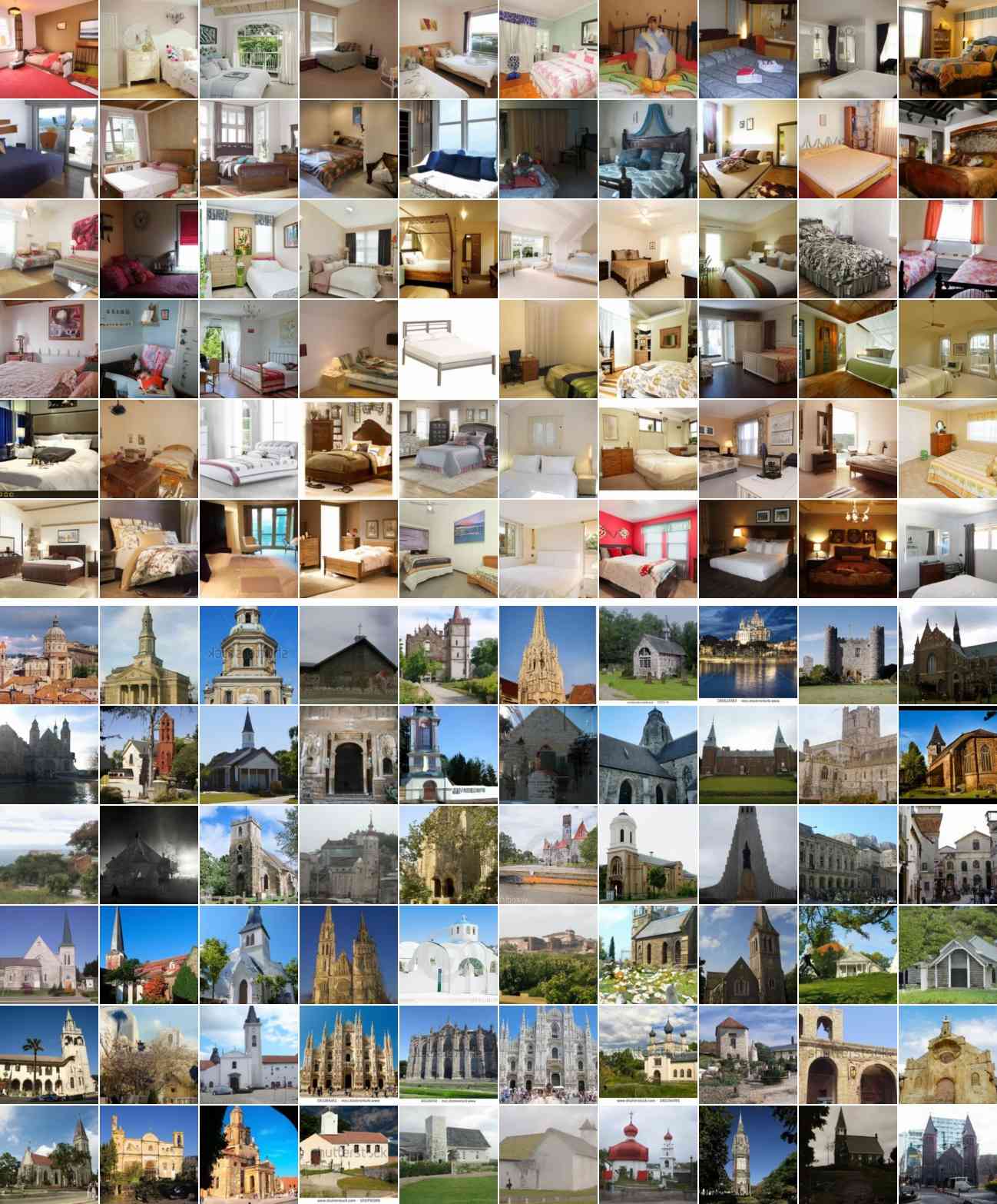
While the main results of this work are on class-conditional ImageNet generation, here we study the effectiveness of non-truncated conditioning augmentation for a 64$\times$64$\to$128$\times$128 cascading pipeline on the LSUN Bedroom and Church datasets (Yu et al., 2015) in order to verify that conditioning augmentation is not an ImageNet-specific method. LSUN Bedroom and Church are two separate unconditional datasets that do not have any class labels, so our study here additionally verifies the effectiveness of conditioning augmentation for unconditional generation.

Table 5 displays our LSUN sample quality results, which confirm that a nonzero amount of conditioning augmentation is beneficial to sample quality. (The relatively large FID scores between generated examples and the validation sets are explained by the fact that the LSUN Church and Bedroom validation sets are extremely small, consisting of only 300 examples each.) We observe a similar effect as our ImageNet results in Table 3(b): because the super-resolution model is conditioned on base model samples, the sample quality improves then degrades non-monotonically as the truncation time $s$ is increased. See Section A for examples of images generated by our LSUN models.

Conditioning	FID vs train	FID vs validation
LSUN Bedroom
$s=0$	2.30	40.68
$s=251$	2.06	40.47
$s=501$	2.08	40.44
$s=751$	2.14	40.45
$s=1001$	2.18	40.53
$s=1251$	2.24	40.58
$s=1501$	2.28	40.58
LSUN Church
$s=0$	3.29	42.21
$s=251$	2.97	42.14
$s=501$	2.93	42.17
$s=751$	2.89	42.20
$s=1001$	2.86	42.26
$s=1251$	2.83	42.28
$s=1501$	2.84	42.31

Table 5: 128$\times$128 LSUN sample quality: non-truncated conditioning augmentation for a 64$\times$64$\to$128$\times$128 cascading pipeline using the base model for low resolution conditioning.

5 Related Work

One way to formulate cascaded diffusion models is to modify the original diffusion formalism of a forward process $q({𝐱}_{0:T})$ at single resolution so that the transition $q({𝐱}_t|{𝐱}_{t-1})$ performs downsampling at certain intermediate timesteps, for example at $t\in S≔\{T/4,2T/4,3T/4\}$. The reverse process would then be required to perform upsampling at those timesteps, similar to our cascaded models here. However, there is no guarantee that the reverse transitions at the timesteps in $S$ are conditional Gaussian, unlike the guarantee for reverse transitions at other timesteps for sufficiently slow diffusion. By contrast, our cascaded diffusion model construction dedicates entire conditional diffusion models for these upsampling steps, so it is specified more flexibly.

Recent interest in diffusion models (Sohl-Dickstein et al., 2015) started with work connecting diffusion models to denoising score matching over multiple noise scales (Ho et al., 2020; Song and Ermon, 2019). There have been a number of improvements and alternatives proposed to the diffusion framework, for example generalization to continuous time (Song et al., 2021b), deterministic sampling (Song et al., 2021a), adversarial training (Jolicoeur-Martineau et al., 2021), and others (Gao et al., 2021). For simplicity, we base our models on DDPM (Ho et al., 2020) with modifications from Improved DDPM (Nichol and Dhariwal, 2021) to stay close to the original diffusion framework.

Cascading pipelines have been investigated in work on VQ-VAEs (van den Oord et al., 2016c; Razavi et al., 2019) and autoregressive models (Menick and Kalchbrenner, 2019). Cascading pipelines have also been investigated for diffusion models, such as SR3 (Saharia et al., 2021), Improved DDPM (Nichol and Dhariwal, 2021), and concurrently in ADM (Dhariwal and Nichol, 2021). Our work here focuses on improving cascaded diffusion models for ImageNet generation and is distinguished by the extensive study on conditioning augmentation and deeper cascading pipelines. Our conditioning augmentation work also resembles scheduled sampling in autoregressive sequence generation (Bengio et al., 2015), where noise is used to alleviate the mismatch between train and inference conditions.

Concurrent work (Dhariwal and Nichol, 2021) showed that diffusion models are capable of generating high quality ImageNet samples using an improved architecture, named ADM, and a classifier guidance technique in which a class-conditional diffusion model sampler is modified to simultaneously take gradient steps to maximize the score of an extra trained image classifier. By contrast, our work focuses solely on improving sample quality by cascading, so we avoid introducing extra model elements such as the image classifier. We are interested in avoiding classifier guidance because the FID and Inception score sample quality metrics that we use to evaluate our models are themselves computed on activations of an image classifier trained on ImageNet, and therefore classifier guidance runs the risk of cheating these metrics.

Avoiding classifier guidance comes at the expense of using thousands of diffusion timesteps in our low resolution models, where ADM uses hundreds. ADM with classifier guidance outperforms our models in terms of FID and Inception scores, while our models outperform ADM without classifier guidance as reported by Dhariwal and Nichol. Our work is a showcase of the effectiveness of cascading alone in a pure generative model, and since classifier guidance and cascading complement each other as techniques to improve sample quality and can be applied together, we expect classifier guidance would improve our results too.

6 Conclusion

We have shown that cascaded diffusion models are capable of outperforming state-of-the-art generative models on the ImageNet class-conditional generation benchmark when paired with conditioning augmentation, our technique of introducing data augmentation into the conditioning information of super-resolution models. Our models outperform BigGAN-deep and VQ-VAE-2 as measured by FID score and classification accuracy score. We found that conditioning augmentation helps sample quality because it combats compounding error in cascading pipelines due to train-test mismatch in super-resolution models, and we proposed practical methods to train and test models amortized over varying levels of conditioning augmentation.

Although there could be negative impact of our work in the form of malicious uses of image generation, our work has the potential to improve beneficial downstream applications such as data compression while advancing the state of knowledge in fundamental machine learning problems. We see our results as a conceptual study of the image synthesis capabilities of diffusion models in their original form with minimal extra techniques, and we hope our work serves as inspiration for future advances in the capabilities of diffusion models.

Acknowledgments

We thank Jascha Sohl-Dickstein, Douglas Eck and the Google Brain team for feedback, research discussions and technical assistance.

A Samples

Figure 11: Samples from classes with best relative classification accuracy score. Each row represents a specific ImageNet class. Classes from top to bottom - Tiger Cat (282), Gong (577), Coffee Mug (504), Squirrel Monkey (382), Miniature Schnauzer (196) and Corn (987).

Figure 12: Samples from classes with worst relative classification accuracy score. Each row represents a specific ImageNet class. Classes from top to bottom - Letter Opener (623), Plate (923), Overskirt (689), Tobacco Shop (860), Black-and-tan Coonhound (165) and Bathtub (435).

Figure 13: Samples from LSUN 128x128: bedroom subset (first six rows) and church subset (last six rows).

B Hyperparameters

B.1 ImageNet

Here we give the hyperparameters of the models in our ImageNet cascading pipelines. Each model in the pipeline is described by its diffusion process, its neural network architecture, and its training hyperparameters. Architecture hyperparameters, such as the base channel count and the list of channel multipliers per resolution, refer to hyperparameters of the U-Net in DDPM and related models (Ho et al., 2020; Nichol and Dhariwal, 2021; Saharia et al., 2021; Salimans et al., 2017). The cosine noise schedule and the hybrid loss method of learning reverse process variances are from Improved DDPM (Nichol and Dhariwal, 2021). Some models are conditioned on ${\overline{\alpha }}_t$ for post-training sampler tuning (Chen et al., 2021; Saharia et al., 2021).

32$\times$32 base model

• Architecture – Base channels: 256 – Channel multipliers: 1, 2, 3, 4 – Residual blocks per resolution: 6 – Attention resolutions: 8, 16 – Attention heads: 4 • Training – Optimizer: Adam – Batch size: 2048 – Learning rate: 1e-4 – Steps: 700000 – Dropout: 0.1 – EMA: 0.9999 – Hardware: 256 TPU-v3 cores • Diffusion – Timesteps: 4000 – Noise schedule: cosine – Learned variances: yes – Loss: hybrid

32$\times$32$\to$64$\times$64 super-resolution

• Architecture – Base channels: 256 – Channel multipliers: 1, 2, 3, 4 – Residual blocks per resolution: 5 – Attention resolutions: 8, 16 – Attention heads: 4 • Training – Optimizer: Adam – Batch size: 2048 – Learning rate: 1e-4 – Steps: 400000 – Dropout: 0.1 – EMA: 0.9999 – Hardware: 256 TPU-v3 cores • Diffusion – Timesteps: 4000 – Noise schedule: cosine – Learned variances: yes – Loss: hybrid

64$\times$64$\to$128$\times$128 super-resolution

• Architecture – Base channels: 128 – Channel multipliers: 1, 2, 4, 8, 8 – Residual blocks per resolution: 3 – Attention resolutions: 16 – Attention heads: 1 • Training – Optimizer: Adam – Batch size: 1024 – Learning rate: 1e-4 – Steps: 500000 – Dropout: 0.0 – EMA: 0.9999 – Hardware: 128 TPU-v3 cores • Diffusion (Training) – Timesteps: 2000 – Noise schedule: linear – Learned variances: no – Loss: simple – Continuous noise conditioning • Diffusion (Inference) – Timesteps: 100 – Noise schedule: linear

64$\times$64$\to$256$\times$256 super-resolution

• Architecture – Base channels: 128 – Channel multipliers: 1, 2, 4, 4, 8, 8 – Residual blocks per resolution: 3 – Attention resolutions: 16 – Attention heads: 1 • Training – Optimizer: Adam – Batch size: 1024 – Learning rate: 1e-4 – Steps: 500000 – Dropout: 0.0 – EMA: 0.9999 – Hardware: 128 TPU-v3 cores • Diffusion (Training) – Timesteps: 2000 – Noise schedule: linear – Learned variances: no – Loss: simple – Continuous noise conditioning • Diffusion (Inference) – Timesteps: 100 – Noise schedule: linear

B.2 LSUN

Here we give the hyperparameters of our LSUN Bedroom and Church pipelines. We used the same hyperparameters for both datasets.

64$\times$64 base model

• Architecture – Base channels: 128 – Channel multipliers: 1, 2, 3, 4 – Residual blocks per resolution: 3 – Attention resolutions: 8, 16, 32 – Attention heads dimension: 64 • Training – Optimizer: Adam – Batch size: 2048 – Learning rate: 3e-4 – Steps: 100000 – Dropout: 0.1 – EMA: 0.9999 – Hardware: 64 TPU-v3 cores • Diffusion (Training) – Noise schedule: cosine – Learned variances: no – Loss: simple – Continuous noise conditioning • Diffusion (Inference) – Timesteps: 256 – Noise schedule: cosine

64$\times$64$\to$128$\times$128 super-resolution

• Architecture – Base channels: 64 – Channel multipliers: 1, 2, 4, 6, 8 – Residual blocks per resolution: 3 – Attention resolutions: 8, 16, 32 – Attention heads dimension: 64 • Training – Optimizer: Adam – Batch size: 1024 – Learning rate: 2e-4 – Steps: 220000 – Dropout: 0.1 – EMA: 0.9999 – Hardware: 64 TPU-v3 cores • Diffusion (Training) – Noise schedule: cosine – Learned variances: no – Loss: simple – Continuous noise conditioning • Diffusion (Inference) – Timesteps: 256 – Noise schedule: cosine

References

- Bengio et al. (2015) S. Bengio, O. Vinyals, N. Jaitly, and N. Shazeer. Scheduled sampling for sequence prediction with recurrent neural networks. Advances in Neural Information Processing Systems, 2015.
- Brock et al. (2019) A. Brock, J. Donahue, and K. Simonyan. Large scale GAN training for high fidelity natural image synthesis. In International Conference on Learning Representations, 2019.
- Chen et al. (2021) N. Chen, Y. Zhang, H. Zen, R. J. Weiss, M. Norouzi, and W. Chan. WaveGrad: Estimating gradients for waveform generation. International Conference on Learning Representations, 2021.
- De Fauw et al. (2019) J. De Fauw, S. Dieleman, and K. Simonyan. Hierarchical autoregressive image models with auxiliary decoders. arXiv preprint arXiv:1903.04933, 2019.
- Dhariwal and Nichol (2021) P. Dhariwal and A. Nichol. Diffusion models beat gans on image synthesis. arXiv preprint arXiv:2105.05233, 2021.
- Dinh et al. (2017) L. Dinh, J. Sohl-Dickstein, and S. Bengio. Density estimation using Real NVP. International Conference on Learning, 2017.
- Gao et al. (2021) R. Gao, Y. Song, B. Poole, Y. N. Wu, and D. P. Kingma. Learning energy-based models by diffusion recovery likelihood. International Conference on Learning Representations, 2021.
- Goodfellow et al. (2014) I. Goodfellow, J. Pouget-Abadie, M. Mirza, B. Xu, D. Warde-Farley, S. Ozair, A. Courville, and Y. Bengio. Generative adversarial nets. In Advances in Neural Information Processing Systems, pages 2672–2680, 2014.
- Heusel et al. (2017) M. Heusel, H. Ramsauer, T. Unterthiner, B. Nessler, and S. Hochreiter. GANs trained by a two time-scale update rule converge to a local Nash equilibrium. In Advances in Neural Information Processing Systems, pages 6626–6637, 2017.
- Ho et al. (2019) J. Ho, X. Chen, A. Srinivas, Y. Duan, and P. Abbeel. Flow++: Improving flow-based generative models with variational dequantization and architecture design. In International Conference on Machine Learning, 2019.
- Ho et al. (2020) J. Ho, A. Jain, and P. Abbeel. Denoising diffusion probabilistic models. In Advances in Neural Information Processing Systems, pages 6840–6851, 2020.
- Jolicoeur-Martineau et al. (2021) A. Jolicoeur-Martineau, R. Piché-Taillefer, R. T. d. Combes, and I. Mitliagkas. Adversarial score matching and improved sampling for image generation. International Conference on Learning Representations, 2021.
- Kingma and Dhariwal (2018) D. P. Kingma and P. Dhariwal. Glow: Generative flow with invertible 1x1 convolutions. In Advances in Neural Information Processing Systems, pages 10215–10224, 2018.
- Kingma and Welling (2014) D. P. Kingma and M. Welling. Auto-encoding variational Bayes. International Conference on Learning Representations, 2014.
- Kong et al. (2021) Z. Kong, W. Ping, J. Huang, K. Zhao, and B. Catanzaro. DiffWave: A Versatile Diffusion Model for Audio Synthesis. International Conference on Learning Representations, 2021.
- Menick and Kalchbrenner (2019) J. Menick and N. Kalchbrenner. Generating high fidelity images with subscale pixel networks and multidimensional upscaling. In International Conference on Learning Representations, 2019.
- Nichol and Dhariwal (2021) A. Nichol and P. Dhariwal. Improved denoising diffusion probabilistic models. International Conference on Machine Learning, 2021.
- Ranzato et al. (2016) M. Ranzato, S. Chopra, M. Auli, and W. Zaremba. Sequence level training with recurrent neural networks. International Conference on Learning Representations, 2016.
- Ravuri and Vinyals (2019) S. Ravuri and O. Vinyals. Classification Accuracy Score for Conditional Generative Models. In Advances in Neural Information Processing Systems, volume 32, 2019.
- Razavi et al. (2019) A. Razavi, A. van den Oord, and O. Vinyals. Generating diverse high-fidelity images with VQ-VAE-2. In Advances in Neural Information Processing Systems, pages 14837–14847, 2019.
- Ronneberger et al. (2015) O. Ronneberger, P. Fischer, and T. Brox. U-Net: Convolutional networks for biomedical image segmentation. In International Conference on Medical Image Computing and Computer-Assisted Intervention, pages 234–241. Springer, 2015.
- Russakovsky et al. (2015) O. Russakovsky, J. Deng, H. Su, J. Krause, S. Satheesh, S. Ma, Z. Huang, A. Karpathy, A. Khosla, M. Bernstein, et al. ImageNet large scale visual recognition challenge. International Journal of Computer Vision, 115(3):211–252, 2015.
- Saharia et al. (2021) C. Saharia, J. Ho, W. Chan, T. Salimans, D. J. Fleet, and M. Norouzi. Image super-resolution via iterative refinement. arXiv preprint arXiv:2104.07636, 2021.
- Salimans et al. (2016) T. Salimans, I. Goodfellow, W. Zaremba, V. Cheung, A. Radford, and X. Chen. Improved techniques for training gans. In Advances in Neural Information Processing Systems, pages 2234–2242, 2016.
- Salimans et al. (2017) T. Salimans, A. Karpathy, X. Chen, and D. P. Kingma. PixelCNN++: Improving the PixelCNN with discretized logistic mixture likelihood and other modifications. In International Conference on Learning Representations, 2017.
- Sohl-Dickstein et al. (2015) J. Sohl-Dickstein, E. Weiss, N. Maheswaranathan, and S. Ganguli. Deep unsupervised learning using nonequilibrium thermodynamics. In International Conference on Machine Learning, pages 2256–2265, 2015.
- Song et al. (2021a) J. Song, C. Meng, and S. Ermon. Denoising diffusion implicit models. International Conference on Learning Representations, 2021a.
- Song and Ermon (2019) Y. Song and S. Ermon. Generative modeling by estimating gradients of the data distribution. In Advances in Neural Information Processing Systems, pages 11895–11907, 2019.
- Song and Ermon (2020) Y. Song and S. Ermon. Improved techniques for training score-based generative. Advances in Neural Information Processing Systems, 2020.
- Song et al. (2021b) Y. Song, J. Sohl-Dickstein, D. P. Kingma, A. Kumar, S. Ermon, and B. Poole. Score-based generative modeling through stochastic differential equations. International Conference on Learning Representations, 2021b.
- van den Oord et al. (2016a) A. van den Oord, S. Dieleman, H. Zen, K. Simonyan, O. Vinyals, A. Graves, N. Kalchbrenner, A. Senior, and K. Kavukcuoglu. WaveNet: A generative model for raw audio. arXiv preprint arXiv:1609.03499, 2016a.
- van den Oord et al. (2016b) A. van den Oord, N. Kalchbrenner, and K. Kavukcuoglu. Pixel recurrent neural networks. International Conference on Machine Learning, 2016b.
- van den Oord et al. (2016c) A. van den Oord, N. Kalchbrenner, O. Vinyals, L. Espeholt, A. Graves, and K. Kavukcuoglu. Conditional image generation with PixelCNN decoders. In Advances in Neural Information Processing Systems, pages 4790–4798, 2016c.
- van den Oord et al. (2017) A. van den Oord, O. Vinyals, and K. Kavukcuoglu. Neural discrete representation learning. Advances in Neural Information Processing Systems, 2017.
- Wu et al. (2019) Y. Wu, J. Donahue, D. Balduzzi, K. Simonyan, and T. Lillicrap. Logan: Latent optimisation for generative adversarial networks. arXiv preprint arXiv:1912.00953, 2019.
- Yu et al. (2015) F. Yu, Y. Zhang, S. Song, A. Seff, and J. Xiao. LSUN: Construction of a large-scale image dataset using deep learning with humans in the loop. arXiv preprint arXiv:1506.03365, 2015.