具有深度语言理解的真实感文本到图像扩散模型

摘要

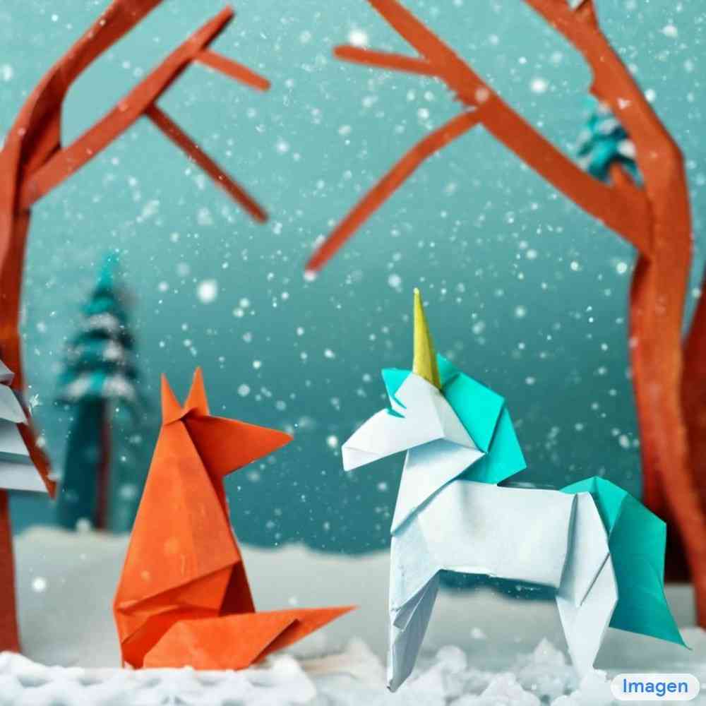
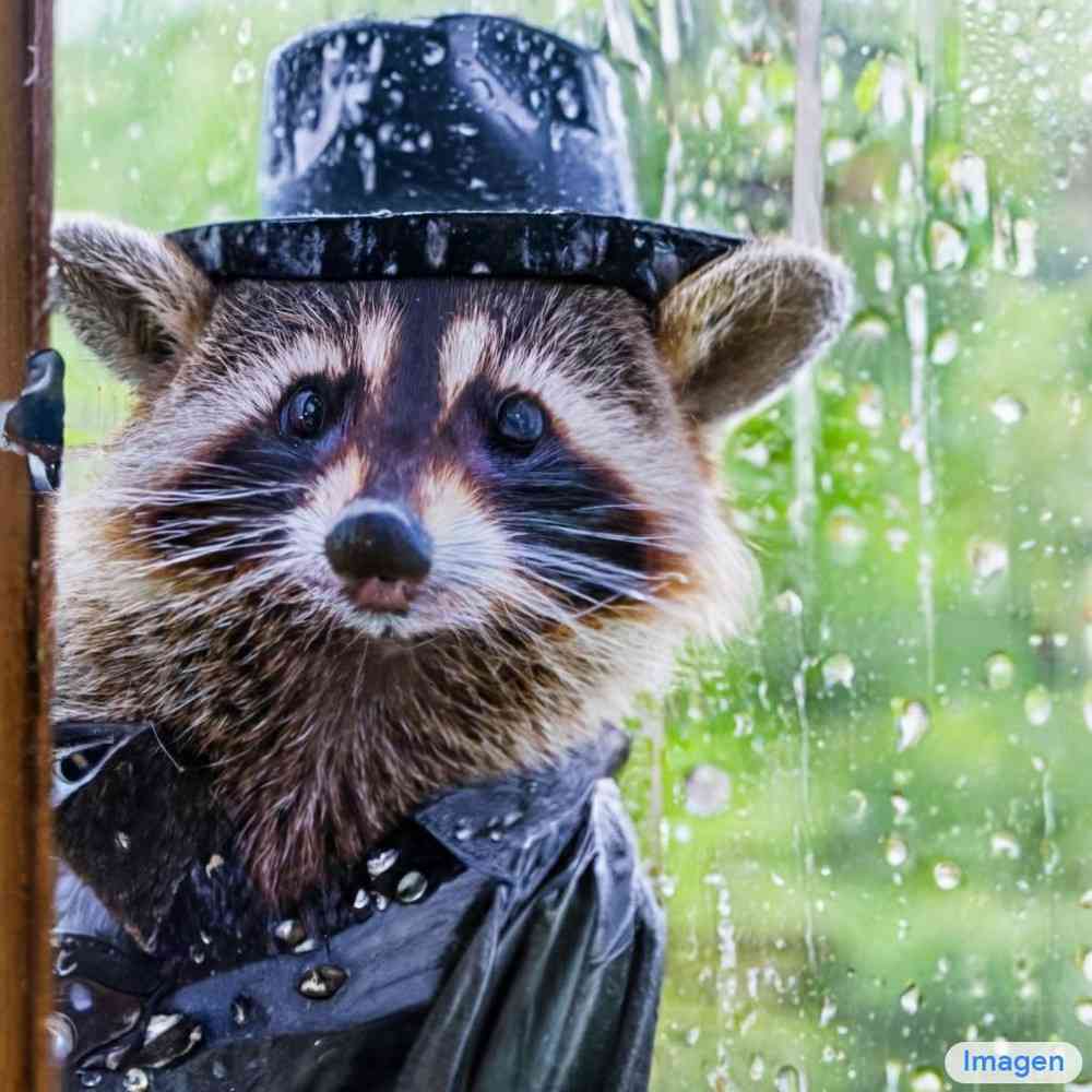
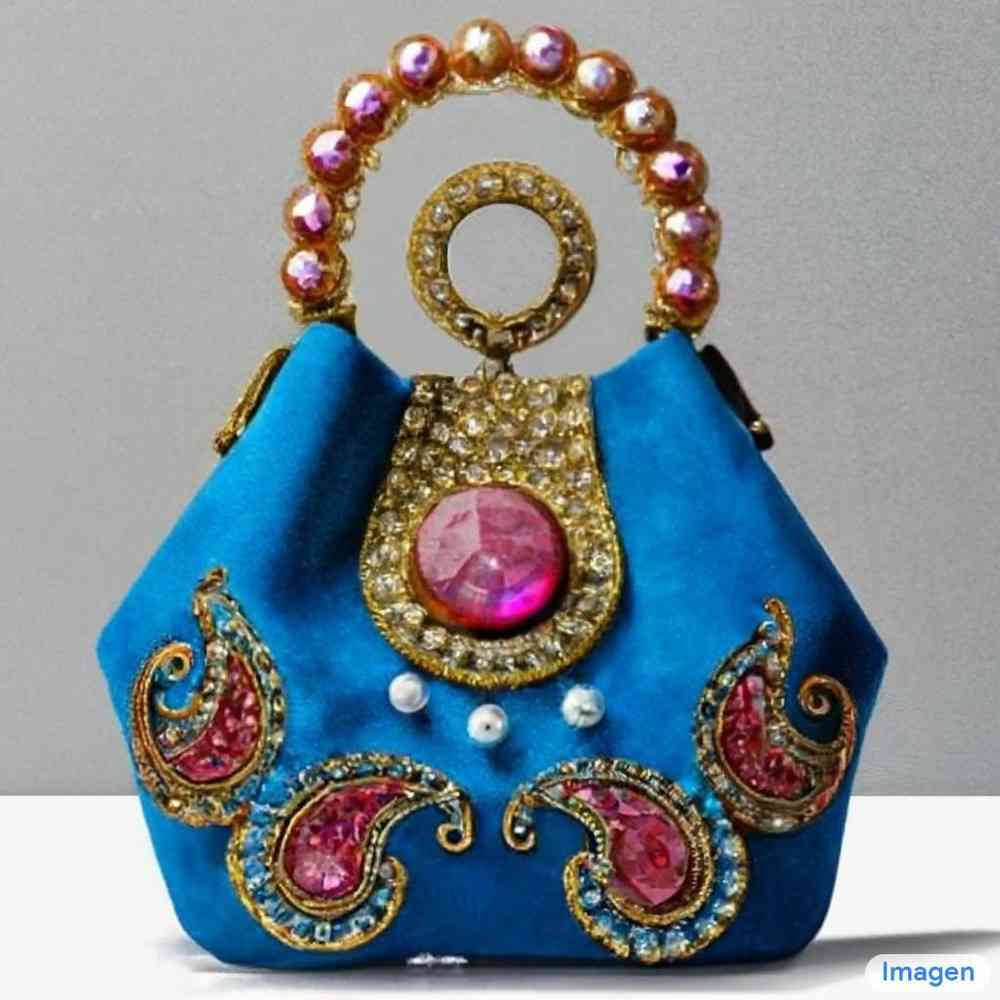
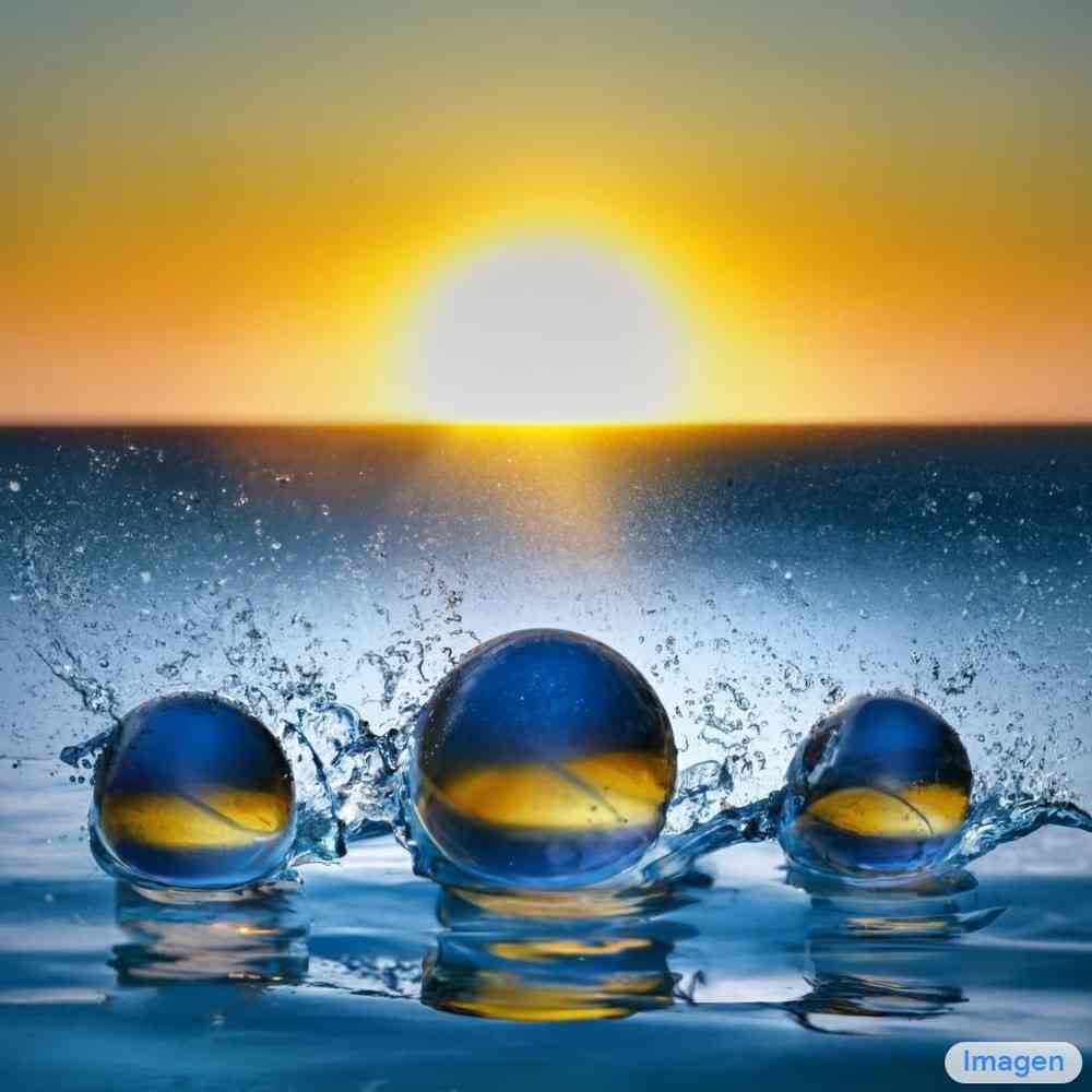
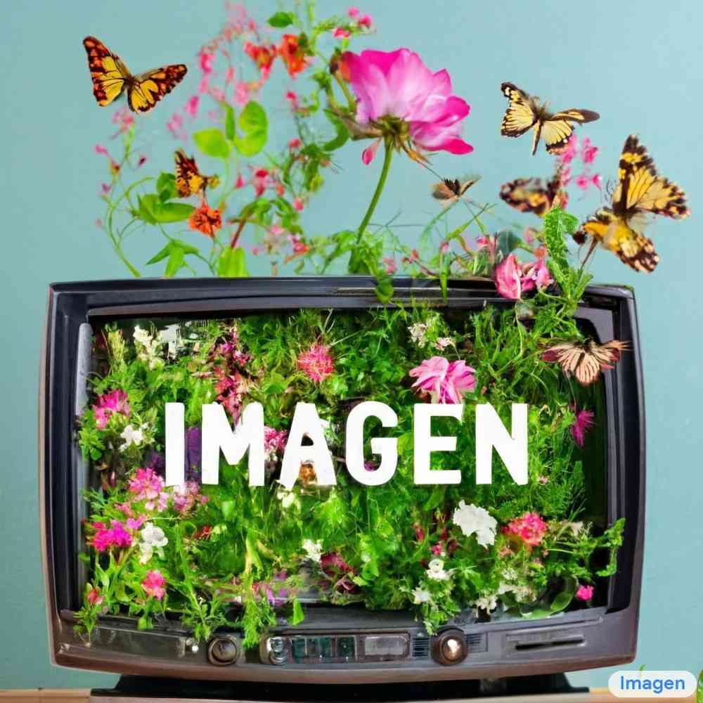
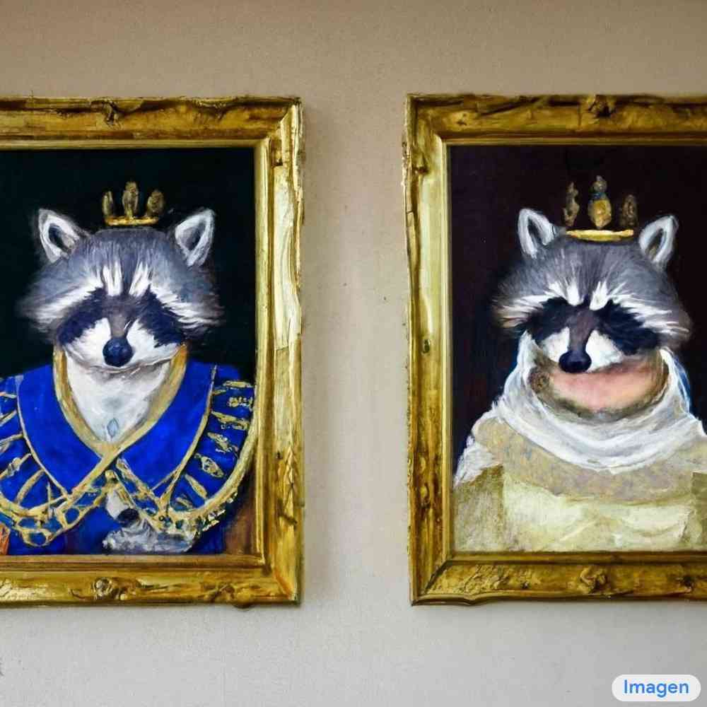
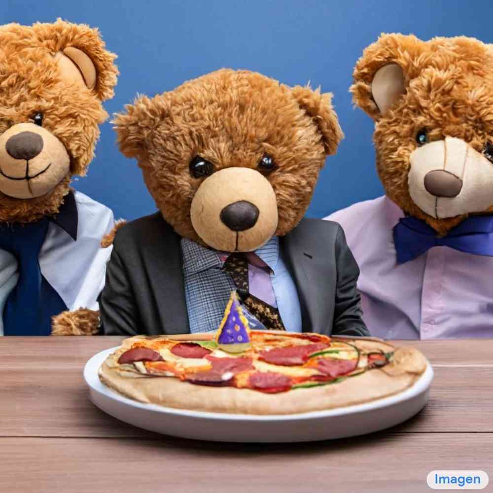
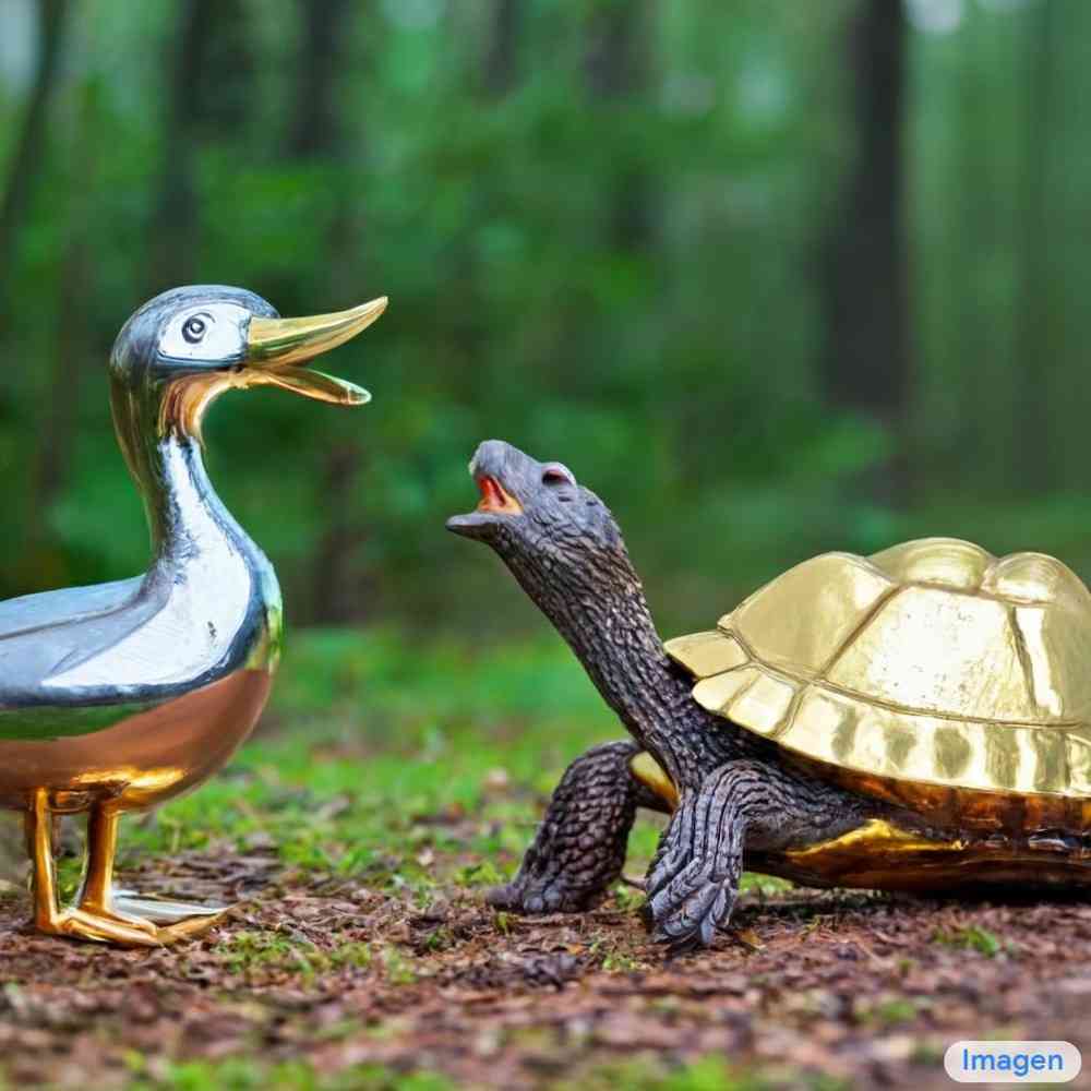
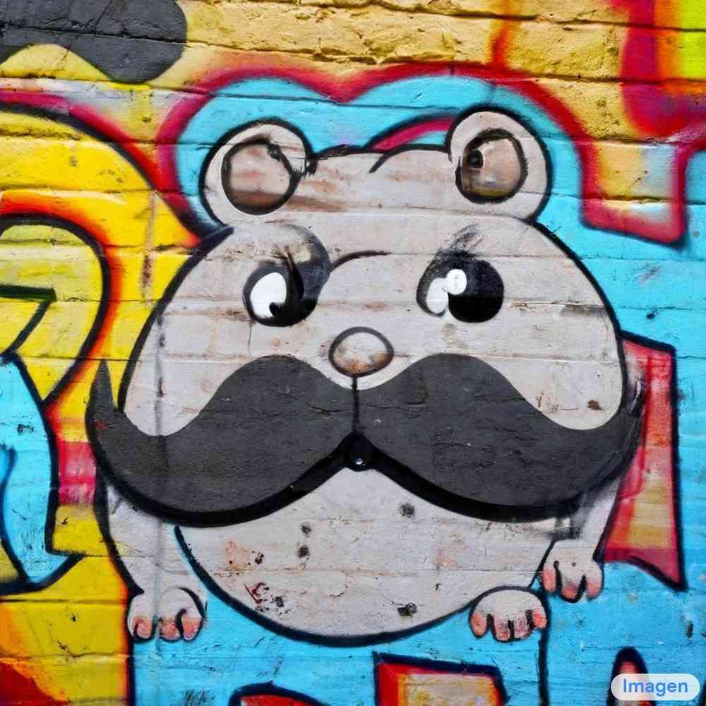
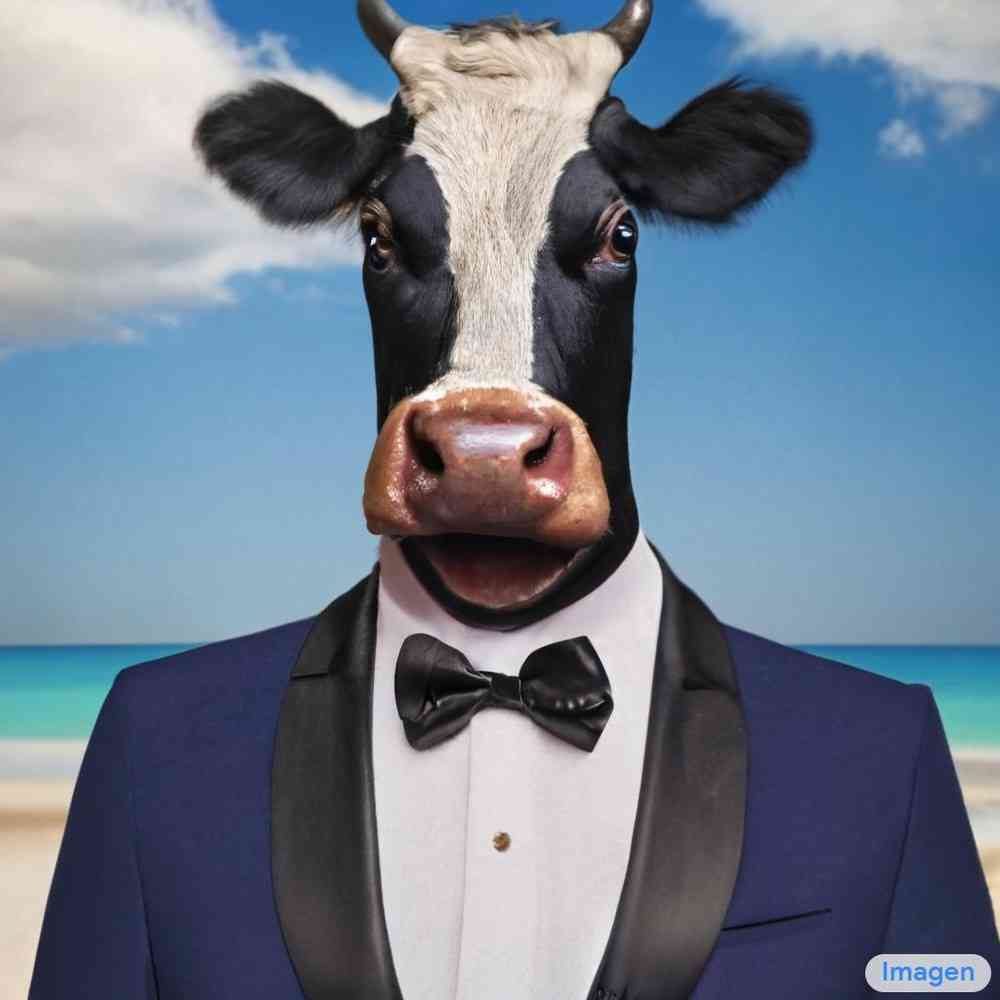
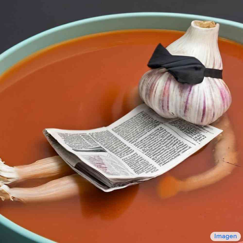
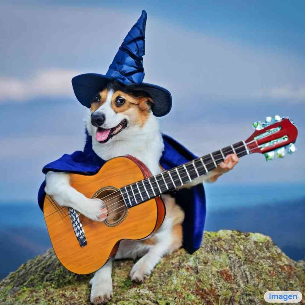
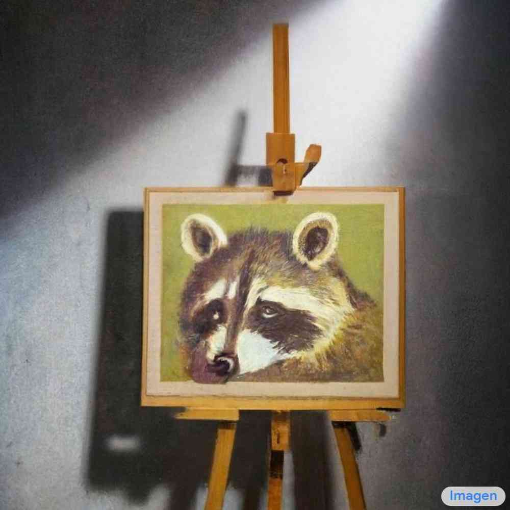
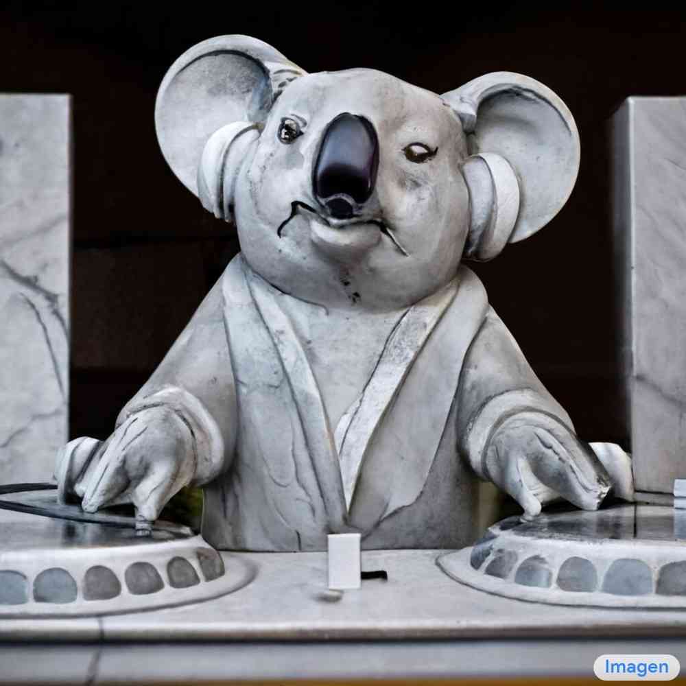
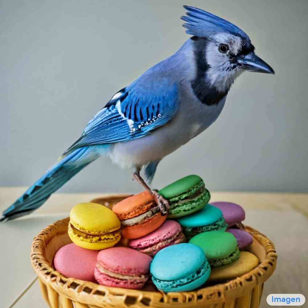
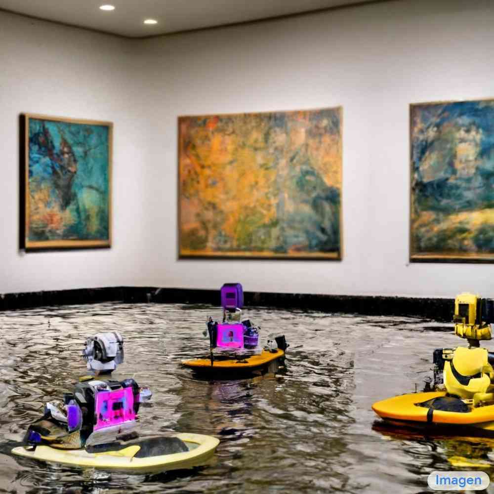
我们推出 Imagen，一种文本到图像的扩散模型，具有前所未有的照片真实感和深层次的语言理解。 Imagen 建立在大型 Transformer 语言模型在理解文本方面的强大功能之上，并依赖于扩散模型在高保真图像生成方面的优势。 我们的关键发现是，在纯文本语料库上进行预训练的通用大型语言模型（例如 T5）在编码文本以进行图像合成方面出奇地有效：增加 Imagen 中语言模型的大小可以大大提高样本保真度和图像文本对齐不仅仅是增加图像扩散模型的尺寸。 Imagen 在 COCO 数据集上达到了新的最先进的 FID 分数 7.27，而无需在 COCO 上进行训练，并且人类评估者发现 Imagen 样本在图像文本对齐方面与 COCO 数据本身相当。 为了更深入地评估文本到图像模型，我们引入了 DrawBench，这是一个全面且具有挑战性的文本到图像模型基准。 通过 DrawBench，我们将 Imagen 与最新的方法（包括 VQ-GAN+CLIP、潜在扩散模型、GLIDE 和 DALL-E 2）进行比较，发现在并排比较中，人类评分者更喜欢 Imagen，无论是在样本方面还是其他模型质量和图像文本对齐。 请参阅 imagen.research.google 了解结果概述。

1简介

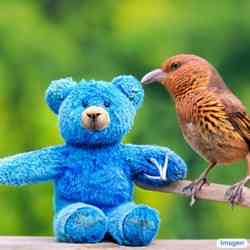
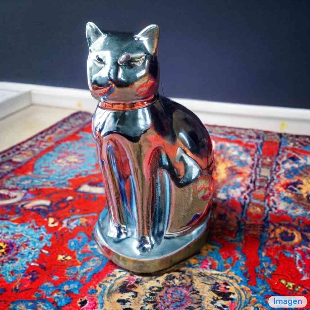
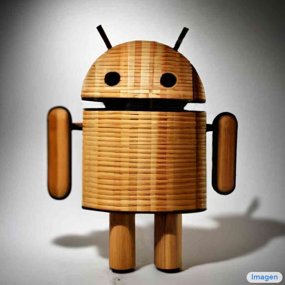
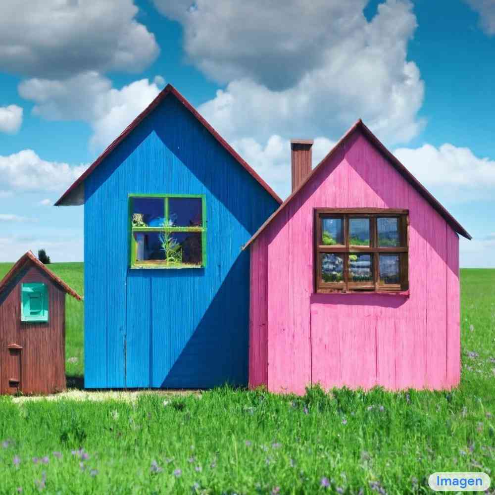
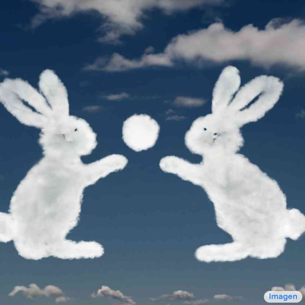
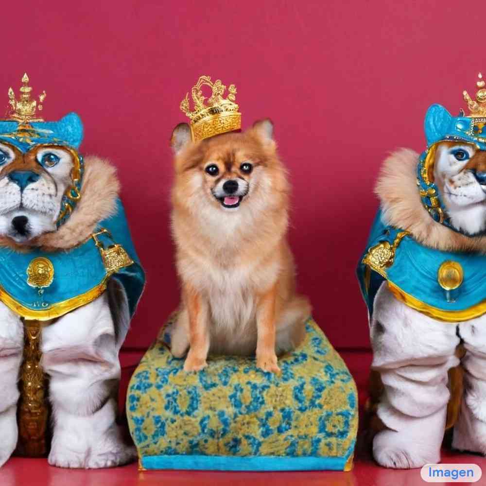
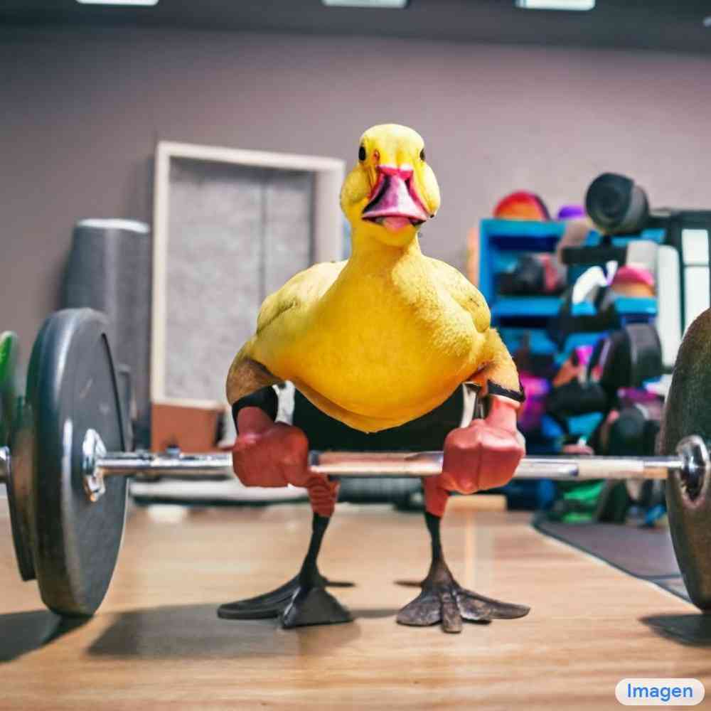
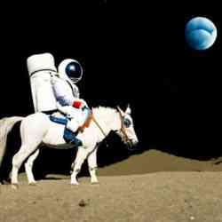
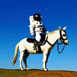
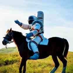
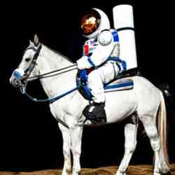
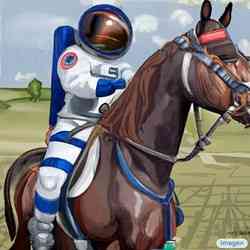
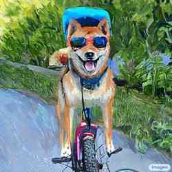
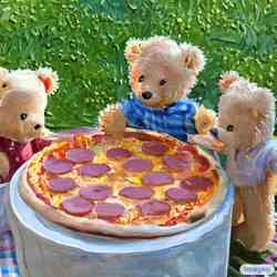
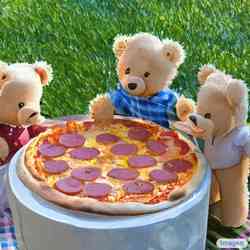
多模态学习最近开始受到关注，其中文本到图像合成[53,12,57]和图像-文本对比学习[49,31,74]最前沿。 这些模型通过创意图像生成[22, 54]和编辑应用程序[21,41,34]改变了研究界并吸引了广泛的公众关注。 为了进一步研究这一研究方向，我们引入了 Imagen，一种文本到图像的扩散模型，它将 Transformer 语言模型 (LM) [15, 52] 的强大功能与高保真扩散模型 [28,29,16,41] 在文本到图像的合成中提供前所未有的真实感和深层次的语言理解。 与之前仅使用图像文本数据进行模型训练 [例如, 53, 41] 的工作相比，Imagen 背后的关键发现是来自大型 LM [52, 15] 的文本嵌入，在纯文本语料库上进行预训练，对于文本到图像的合成非常有效。 请参阅图1了解选定示例。

(a) Sprouts in the shape of text ‘Imagen’ coming out of a fairytale book.

(b) A photo of a Shiba Inu dog with a backpack riding a bike. It is wearing sunglasses and a beach hat.

(c) A high contrast portrait of a very happy fuzzy panda dressed as a chef in a high end kitchen making dough. There is a painting of flowers on the wall behind him.

(d) Teddy bears swimming at the Olympics 400m Butterfly event.

(e) A cute corgi lives in a house made out of sushi.

(f) A cute sloth holding a small treasure chest. A bright golden glow is coming from the chest.

(g) A brain riding a rocketship heading towards the moon.

(h) A dragon fruit wearing karate belt in the snow.

(i) A strawberry mug filled with white sesame seeds. The mug is floating in a dark chocolate sea.

图1： 选择 $1024\times 1024$ Imagen 样本进行各种文本输入。 我们在此图中仅包含真实感图像，并将艺术内容留给附录，因为从技术角度来看，生成真实感图像更具挑战性。 图 A.1、A.2 和 A.3 显示更多示例。

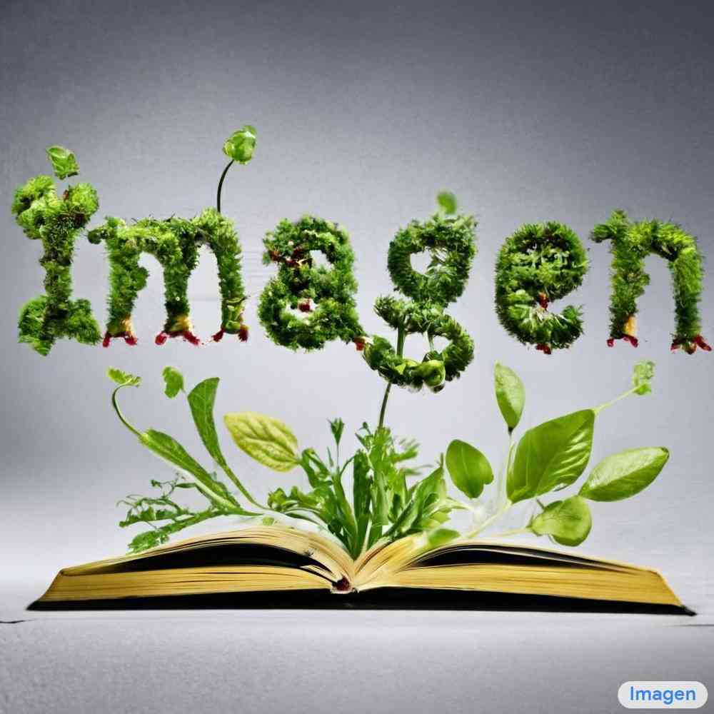
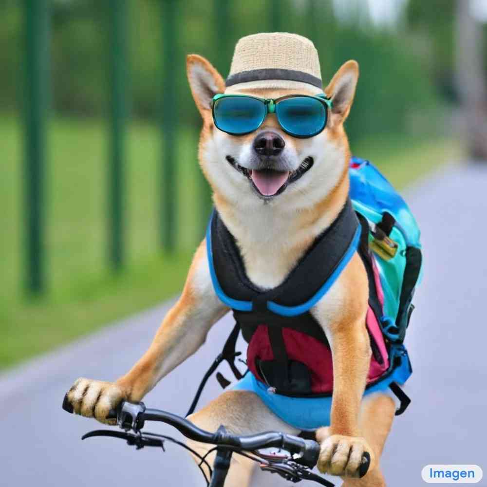
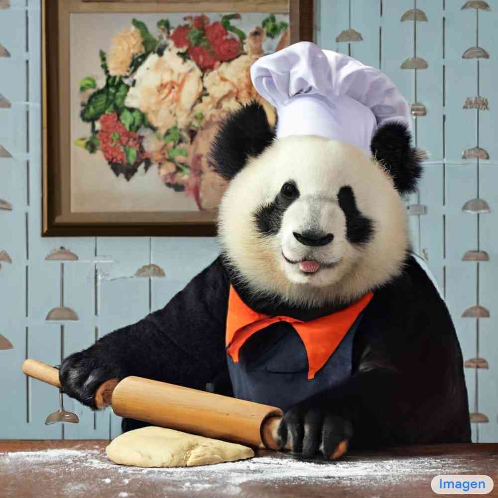
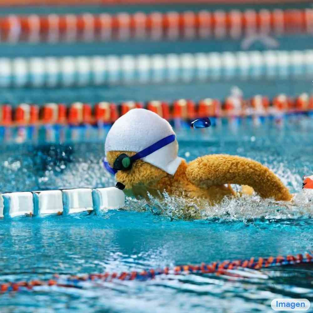
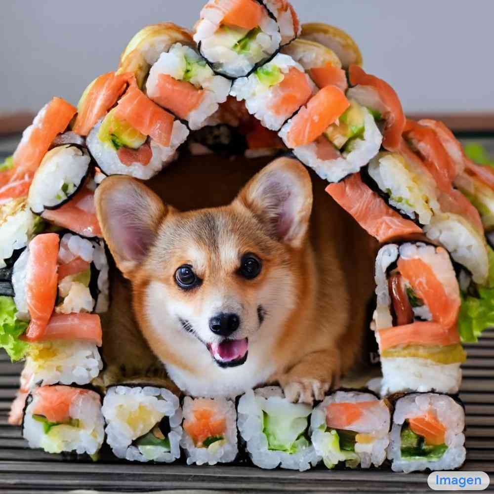
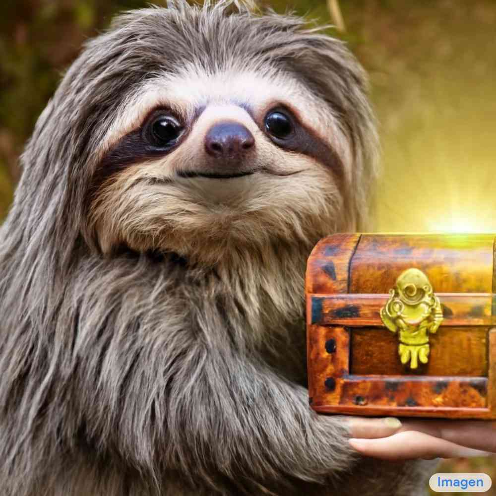
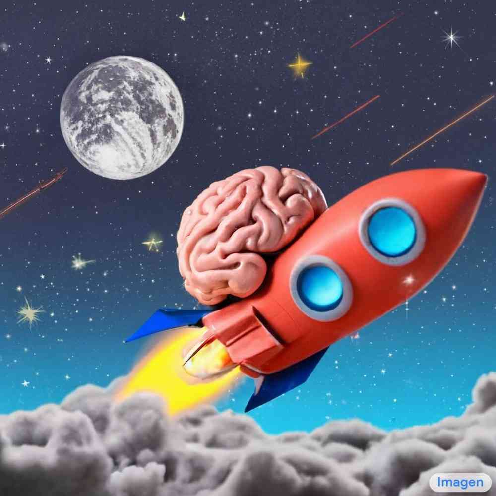
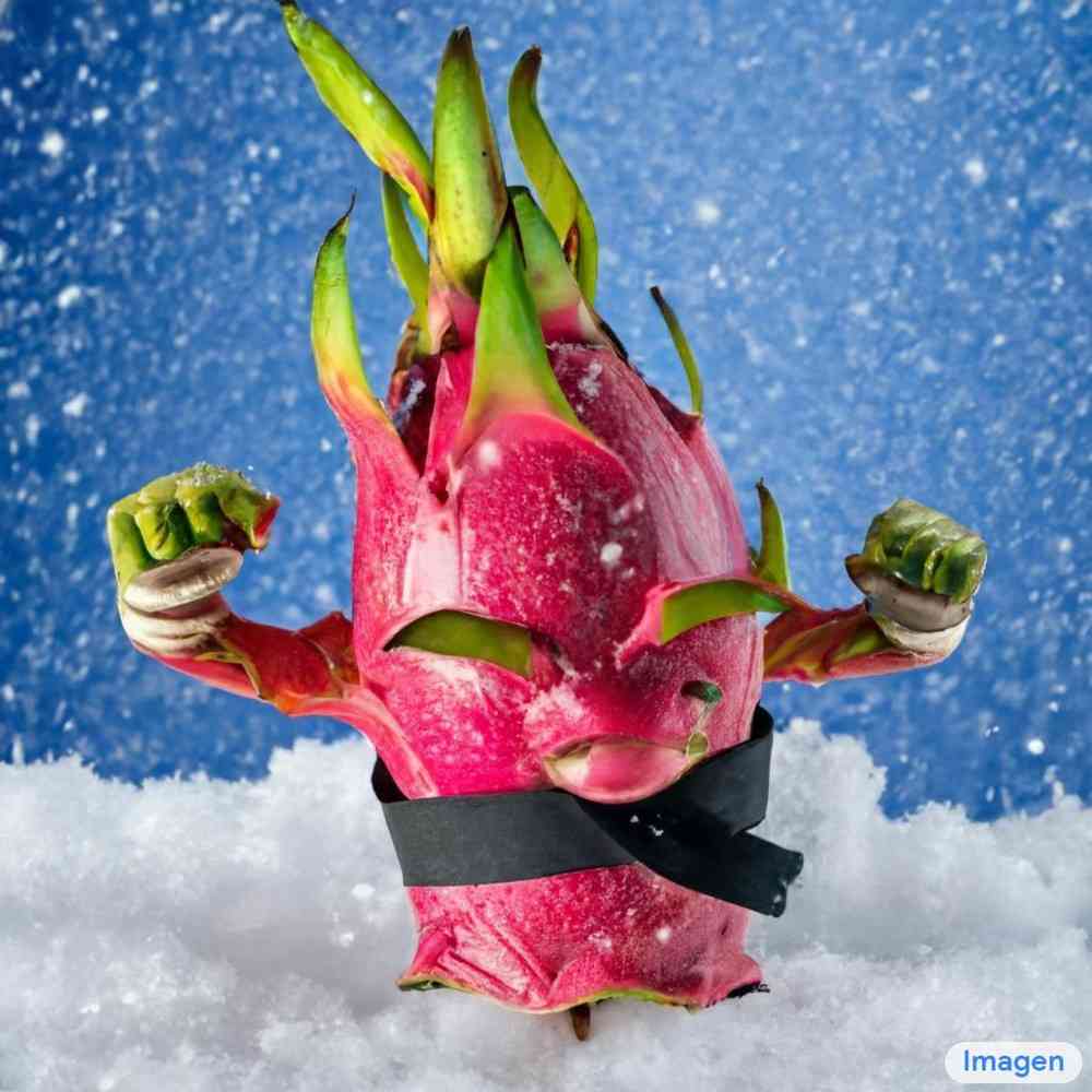
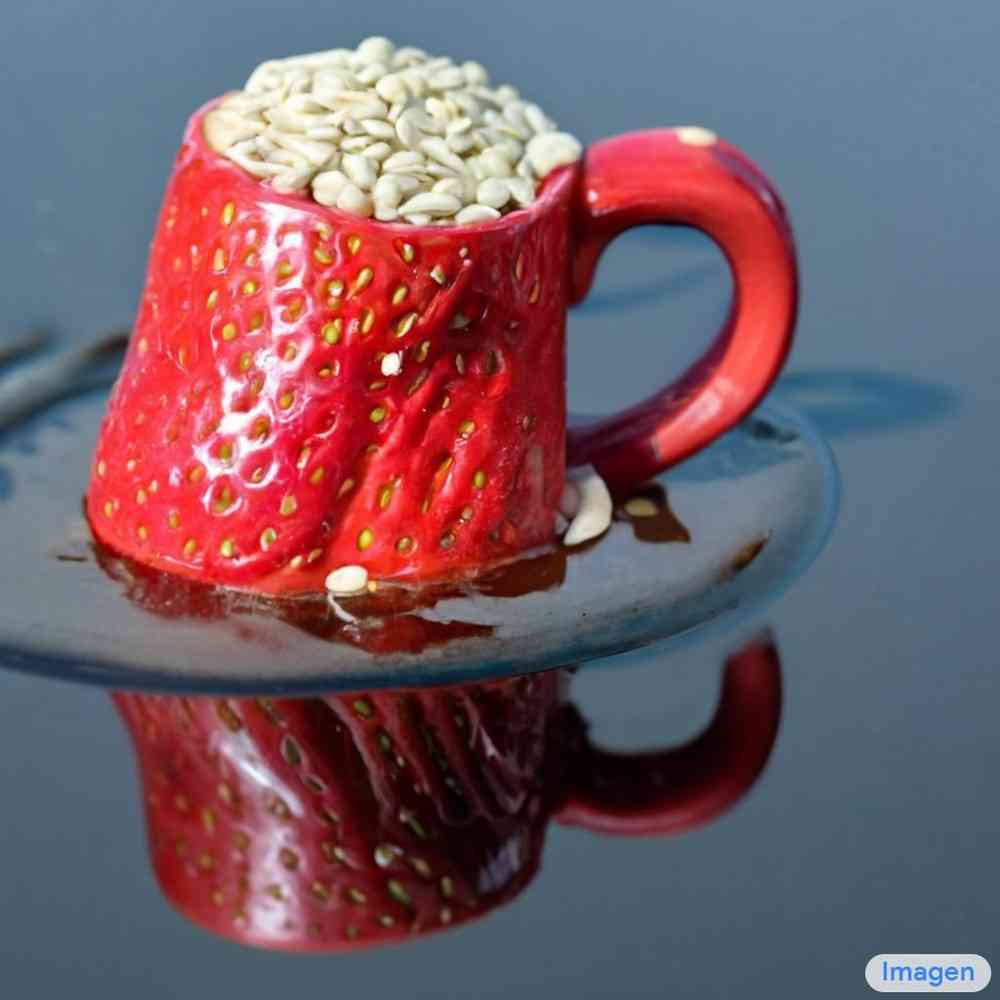
Imagen 包含一个冻结的 T5-XXL [52] 编码器，用于将输入文本映射到一系列嵌入中，以及一个 $64\times 64$ 图像扩散模型，后面是两个超分辨率扩散模型，用于生成$256\times 256$和$1024\times 1024$图像（参见图A.4)。 所有扩散模型都以文本嵌入序列为条件，并使用无分类器指导[27]。 Imagen 依靠新的采样技术来允许使用较大的指导权重，而不会出现之前工作中观察到的样本质量下降的情况，从而产生比以前更高保真度和更好图像文本对齐的图像。

虽然 Imagen 概念简单且易于训练，但它却产生了令人惊讶的强大结果。 Imagen 在 COCO [36] 上的表现优于其他方法，零样本 FID-30K 为 7.27，显着优于先前的工作，例如 GLIDE [41]（12.4）和并发工作DALL-E 2 [54]（10.4）。 我们的零样本 FID 分数也优于在 COCO 上训练的最先进模型，例如 Make-A-Scene [22]（7.6）。 此外，人类评分者表示，从 Imagen 生成的样本在图像文本对齐方面与 COCO 字幕上的参考图像不相上下。

我们推出了 DrawBench，这是一套新的结构化文本提示，用于文本到图像的评估。 DrawBench 通过对文本到图像模型的多维评估来实现更深入的见解，并提供旨在探测模型不同语义属性的文本提示。 这些包括组合性、基数、空间关系、处理复杂文本提示或罕见单词提示的能力，并且还包括创造性提示，这些提示突破了模型生成远远超出训练数据范围的高度难以置信的场景的能力的极限。 通过 DrawBench，广泛的人类评估表明 Imagen 明显优于其他最新方法[57,12,54]。 我们进一步证明了使用大型预训练语言模型 [52] 相对于多模态嵌入（例如 CLIP [49])作为文本编码器的一些明显优势对于图像。

该论文的主要贡献包括：

1. 我们发现，仅在文本数据上训练的大型冻结语言模型对于文本到图像的生成来说是非常有效的文本编码器，并且缩放冻结文本编码器的大小比缩放图像扩散模型的大小更能显着提高样本质量。

2. 我们引入了动态阈值，这是一种新的扩散采样技术，可利用高引导权重并生成比以前更加逼真和详细的图像。

3. 我们重点介绍了几个重要的扩散架构设计选择，并提出了Efficient U-Net，这是一种更简单、收敛速度更快且内存效率更高的新架构变体。

4. 我们实现了新的最先进的 COCO FID 7.27。 人类评估者发现 Imagen 在图像文本对齐方面与参考图像不相上下。

5. 我们推出了 DrawBench，这是一个新的全面且具有挑战性的文本转图像任务评估基准。 在 DrawBench 人类评估中，我们发现 Imagen 优于所有其他工作，包括 DALL-E 2 [54] 的并发工作。

2 图像

Imagen 由一个文本编码器（将文本映射到一系列嵌入）和一系列条件扩散模型（将这些嵌入映射到分辨率不断增加的图像）组成（参见图 A.4 )。 在以下小节中，我们将详细描述每个组件。

2.1 预训练文本编码器

文本到图像模型需要强大的语义文本编码器来捕获任意自然语言文本输入的复杂性和组合性。 在配对图像文本数据上训练的文本编码器是当前文本到图像模型的标准配置；它们可以从头开始训练 [41, 53] 或在图像文本数据 [54] 上进行预训练（例如 CLIP [49]) 。 图像文本训练目标表明这些文本编码器可以对视觉语义和有意义的表示进行编码，特别是与文本到图像生成任务相关。 大型语言模型可以是对文本进行编码以生成文本到图像的另一种选择模型。 大型语言模型（例如 BERT [15]、GPT [47, 48, 7]、T5 [52])的最新进展导致了文本理解和生成能力的飞跃。 语言模型是在比图像文本配对数据大得多的纯文本语料库上进行训练的，因此会接触到非常丰富且广泛分布的文本。 这些模型通常也比当前图像文本模型 [49, 31, 80] 中的文本编码器大得多（例如 PaLM [11] 有 540B 参数，而 CoCa [80] 有一个 $\approx$ 1B 参数文本编码器）。

因此，探索用于文本到图像任务的两个文本编码器系列就变得很自然了。 Imagen 探索预训练的文本编码器：BERT [15]、T5 [51] 和 CLIP [46]。 为了简单起见，我们冻结这些文本编码器的权重。 冻结有几个优点，例如训练嵌入的离线计算，导致文本到图像模型期间的计算或内存占用可以忽略不计。 在我们的工作中，我们发现有一个明确的信念：缩放文本编码器大小可以提高文本到图像生成的质量。 我们还发现，虽然 T5-XXL 和 CLIP 文本编码器在 MS-COCO 等简单基准测试上表现相似，但在 DrawBench 上的图像文本对齐和图像保真度方面，人类评估者更喜欢 T5-XXL 编码器而不是 CLIP 文本编码器，DrawBench 是一组具有挑战性的测试。和作曲提示。 我们建议读者参阅第 4.4 节来了解我们的研究结果摘要，并参考附录 D.1 来了解详细的消解。

2.2 扩散模型和无分类器指导

这里我们简单介绍一下扩散模型；准确的描述在附录A中。扩散模型[63,28,65]是一类生成模型，通过迭代去噪过程将高斯噪声转换为来自学习数据分布的样本。 这些模型可以是有条件的，例如类标签、文本或低分辨率图像[例如16、29、59、58、75、41、54]。 扩散模型 ${\widehat{𝐱}}_{\theta }$ 在以下形式的去噪目标上进行训练

${𝔼}_{𝐱,𝐜,\mathit{ϵ},t}\left[w_t{\Vert {\widehat{𝐱}}_{\theta }({\alpha }_t𝐱+{\sigma }_t\mathit{ϵ},𝐜)-𝐱\Vert }_2^2\right]$ (1)

其中 $(𝐱,𝐜)$ 是数据调节对，$t\sim 𝒰([0,1])$、$\mathit{ϵ}\sim 𝒩(\mathrm{𝟎},𝐈)$ 和 ${\alpha }_t,{\sigma }_t,w_t$ 是影响 $t$ 的函数样品质量。 直观上，${\widehat{𝐱}}_{\theta }$ 被训练为使用平方误差损失将 ${𝐳}_t≔{\alpha }_t𝐱+{\sigma }_t\mathit{ϵ}$ 去噪为 $𝐱$，并加权以强调 $t$ 的某些值。诸如祖先采样器[28]和DDIM [64]等采样都是从纯噪声${𝐳}_1\sim 𝒩(\mathrm{𝟎},𝐈)$开始，迭代生成点${𝐳}_{t_1},\mathrm{\dots },{𝐳}_{t_T}$ ，其中$1=t_1>\mathrm{\cdots }>t_T=0$，噪声内容逐渐减少。 这些点是 $𝐱$ 预测 ${\widehat{𝐱}}_0^t≔{\widehat{𝐱}}_{\theta }({𝐳}_t,𝐜)$ 的函数。

分类器指导[16]是一种在采样期间使用预训练模型$p(𝐜|{𝐳}_t)$的梯度来提高样本质量同时减少条件扩散模型多样性的技术。 无分类器指导 [27]是一种替代技术，它通过随机删除$𝐜$ 使用调整后的 $𝐱$ 预测 $({𝐳}_t-\sigma {\widetilde{\mathit{ϵ}}}_{\theta })/{\alpha }_t$ 执行采样，其中

${\widetilde{\mathit{ϵ}}}_{\theta }({𝐳}_t,𝐜)=w{\mathit{ϵ}}_{\theta }({𝐳}_t,𝐜)+(1-w){\mathit{ϵ}}_{\theta }({𝐳}_t).$ (2)

这里，${\mathit{ϵ}}_{\theta }({𝐳}_t,𝐜)$和${\mathit{ϵ}}_{\theta }({𝐳}_t)$是条件和无条件$\mathit{ϵ}$预测，由${\mathit{ϵ}}_{\theta }≔({𝐳}_t-{\alpha }_t{\widehat{𝐱}}_{\theta })/{\sigma }_t$给出，$w$是指导权重。 设置$w=1$会禁用无分类器指导，而增加$w>1$会增强指导效果。 Imagen 很大程度上依赖于无分类器的指导来实现有效的文本调节。

2.3大型指导重量采样器

我们证实了最近的文本引导扩散工作[16,41,54]的结果，发现增加无分类器引导权重可以改善图像文本对齐，但会损害图像保真度，从而产生高度饱和和不自然的效果图像[27]。 我们发现这是由于高指导权重引起的训练与测试不匹配造成的。 在每个采样步骤$t$,$𝐱$预测${\widehat{𝐱}}_0^t$必须在与训练数据$𝐱$相同的范围内，即在$[-1,1]$，但我们根据经验发现，高指导权重会导致$𝐱$-预测超出这些界限。 这是训练与测试的不匹配，并且由于扩散模型在整个采样过程中迭代地应用于其自身的输出，因此采样过程会产生不自然的图像，有时甚至会发散。 为了解决这个问题，我们研究了静态阈值和动态阈值。 有关技术的参考实现，请参见附录图A.31和附录图A.9 其效果的可视化。

静态阈值：我们将按元素将$𝐱$预测裁剪为$[-1,1]$称为静态阈值。 事实上，这种方法在之前的工作[28]中已被使用但并未强调，并且据我们所知，其重要性尚未在引导抽样的背景下进行研究。 我们发现静态阈值对于具有大引导权重的采样至关重要，并且可以防止生成空白图像。 尽管如此，随着引导权重进一步增加，静态阈值处理仍然会导致图像过饱和且细节较少。

动态阈值：我们引入了一种新的 动态阈值方法：在每个采样步骤中，我们将 $s$ 设置为 ${\widehat{𝐱}}_0^t$ 中某个百分位数的像素绝对值，如果 $s>1$，则我们将 ${\widehat{𝐱}}_0^t$ 设置为 $[-s,s]$ 的阈值范围，然后除以 $s$。动态阈值处理会将饱和像素（接近-1 和 1 的像素）向内推，从而在每一步都主动防止像素饱和。 我们发现动态阈值处理可以显着提高照片真实感以及更好的图像文本对齐效果，特别是在使用非常大的指导权重时。

2.4稳健的级联扩散模型

Imagen 利用基本 $64\times 64$ 模型的管道和两个文本条件超分辨率扩散模型将 $64\times 64$ 生成的图像上采样为 $256\times 256$ 图像，并且然后到 $1024\times 1024$ 图像。 具有噪声调节增强功能的级联扩散模型[29]在逐步生成高保真图像方面非常有效。 此外，通过噪声水平调节使超分辨率模型了解添加的噪声量，可以显着提高样本质量，并有助于提高超分辨率模型的鲁棒性，以处理较低分辨率模型生成的伪影[29 ]。 Imagen 对两种超分辨率模型都使用了噪声调节增强。 我们发现这对于生成高保真图像至关重要。

给定条件低分辨率图像和增强级别（又名 $\mathrm{aug}\mathrm{\_}\mathrm{level}$)（例如，高斯噪声或模糊的强度），我们通过增强破坏低分辨率图像（对应于 $\mathrm{aug}\mathrm{\_}\mathrm{level}$)，并以 $\mathrm{aug}\mathrm{\_}\mathrm{level}$ 为扩散模型的条件。 在训练过程中，$\mathrm{aug}\mathrm{\_}\mathrm{level}$ 是随机选择的，而在推理过程中，我们会扫描它的不同值以找到最佳样本质量。 在我们的例子中，我们使用高斯噪声作为增强形式，并应用方差保留高斯噪声增强，类似于扩散模型中使用的前向过程(附录 A)。 使用$\mathrm{aug}\mathrm{\_}\mathrm{level}\in [0,1]$指定增强级别。 参考伪代码参见图A.32。

2.5神经网络架构

基本模型：我们将[40]中的U-Net架构改编为我们的基本$64\times 64$文本到图像扩散模型。 该网络通过池化嵌入向量以文本嵌入为条件，添加到扩散时间步长嵌入，类似于 [16, 29] 中使用的类嵌入条件方法。 我们通过在多个分辨率的文本嵌入上添加交叉注意力 [57] 来进一步调节整个文本嵌入序列。 我们在部分D.3.1中研究了各种文本调节方法。 此外，我们发现注意力层和池化层中文本嵌入的层归一化[2]有助于显着提高性能。

超分辨率模型：对于$64\times 64\to 256\times 256$超分辨率，我们使用改编自[40, 58]的U-Net模型。 我们对此 U-Net 模型进行了一些修改，以提高内存效率、推理时间和收敛速度（我们的变体的步数/秒比 [40, 58] 中使用的 U-Net 快 2-3 倍>)。 我们将此变体称为Efficient U-Net（有关更多详细信息和比较，请参阅附录B.1)。 我们的 $256\times 256\to 1024\times 1024$ 超分辨率模型在 $1024\times 1024$ 图像的 $64\times 64\to 256\times 256$ 裁剪上进行训练。 为了实现这一点，我们删除了自注意力层，但保留了我们认为至关重要的文本交叉注意力层。 在推理过程中，模型接收完整的 $256\times 256$ 低分辨率图像作为输入，并返回上采样的 $1024\times 1024$ 图像作为输出。 请注意，我们对两个超分辨率模型都使用文本交叉注意。

A brown bird and a blue bear.		One cat and two dogs sitting on the grass.		A sign that says ’NeurIPS’.
A small blue book sitting on a large red book.		A blue coloured pizza.		A wine glass on top of a dog.
A pear cut into seven pieces		A photo of a confused grizzly bear		A small vessel propelled on water
arranged in a ring.		in calculus class.		by oars, sails, or an engine.

图2： Non-cherry 从 DrawBench 中为不同类别的提示挑选了 Imagen 样本。

3 评估文本到图像模型

COCO [36] 验证集是评估监督 [82, 22] 和零样本设置 的文本到图像模型的标准基准[53, 41]。 使用的关键自动化性能指标是用于测量图像保真度的 FID [26] 和用于测量图像文本对齐的 CLIP 分数 [25, 49]。 与之前的工作一致，我们报告了零样本 FID-30K，其中从验证集中随机抽取 30K 提示，并将这些提示生成的模型样本与完整验证集中的参考图像进行比较。 由于引导权重是控制图像质量和文本对齐的重要因素，因此我们使用一系列引导权重的 CLIP 和 FID 分数之间的权衡（或 pareto)曲线来报告大部分消融结果。

FID 和 CLIP 分数都有局限性，例如 FID 与感知质量 [42] 并不完全一致，而 CLIP 在计数 [49] 方面无效。 由于这些限制，我们使用人工评估来评估图像质量和标题相似性，并以真实参考标题-图像对作为基线。 我们使用两种实验范例：

1. 为了探究图像质量，要求评估者使用以下问题在模型生成和参考图像之间进行选择：“哪张图像更逼真（看起来更真实）？”。 我们报告评估者选择模型生成而不是参考图像的次数百分比(偏好率)。

2. 为了探测对齐情况，人类评估者会看到一张图像和一个提示，并询问“标题是否准确地描述了上面的图像？”。 他们必须回答“是”、“某种程度上”或“不是”。 这些回答的得分分别为 100、50 和 0。 这些评级是针对模型样本和参考图像独立获得的，并且均进行报告。

对于这两种情况，我们使用从 COCO 验证集中随机选择的 200 个图像标题对。 向受试者展示了 50 张图像。 我们还使用了交错的“对照”试验，并且仅包含正确回答至少 80% 对照问题的评估者数据。 对于图像质量和图像文本对齐评估，每幅图像分别获得了 73 分和 51 分。

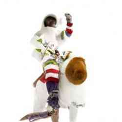
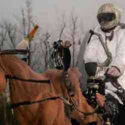
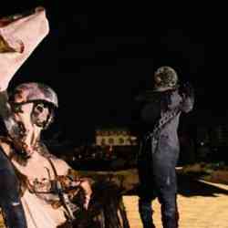
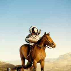
DrawBench：虽然 COCO 是一个有价值的基准，但越来越明显的是，它的提示范围有限，无法轻松提供对模型之间差异的洞察（例如，请参阅第 4.2 [10] 最近的工作提出了一个名为 PaintSkills 的新评估集，用于系统地评估 COCO 之外的视觉推理技能和社会偏见。 出于类似的动机，我们引入了 DrawBench，这是一套全面且具有挑战性的提示，支持文本到图像模型的评估和比较。 DrawBench包含11类提示，测试模型的不同功能，例如忠实渲染不同颜色的能力、对象的数量、空间关系、场景中的文本以及对象之间不寻常的交互。 类别还包括复杂的提示，包括长而复杂的文本描述、生僻单词以及拼写错误的提示。 我们还包括从 DALL-E [53]、Gary Marcus 等人 [38] 和 Reddit 收集的提示集. 在这 11 个类别中，DrawBench 总共包含 200 个提示，在对大型、全面的数据集的需求与足够小以便人类评估仍然可行的需求之间取得了良好的平衡。 （附录C提供了DrawBench的更详细描述。 图 2 显示了来自 DrawBench 和 Imagen 示例的示例提示。）

我们使用DrawBench直接比较不同的模型。 为此，人类评估者会看到两组图像，一组来自模型 A，一组来自模型 B，每组图像都有 8 个样本。 人类评估者被要求在样本保真度和图像文本对齐方面比较模型 A 和模型 B。 他们会做出以下三个选择之一的回应： 更喜欢模型 A；冷漠;或者更喜欢模型 B。

4实验

部分 4.1描述训练细节，部分 4.2和4.3在MS-COCO和DrawBench上分析结果，以及0>部分2> 4.43>1> 总结了我们的消融研究和主要发现。 对于下面的所有实验，图像都是来自 Imagen 的公平随机样本，没有经过后处理或重新排序。

4.1 培训详情

除非另有说明，否则我们将为$64\times 64$文本到图像合成训练 2B 参数模型，为$64\times 64\to 256\times 256$和$256\times 256\to 1024\times 1024$训练 600M 和 400M 参数模型。 分别用于超分辨率。 我们对所有模型使用 2048 的批量大小和 2.5M 训练步骤。 我们的底座使用 256 个 TPU-v4 芯片 $64\times 64$ 型号，以及两种超分辨率型号的 128 个 TPU-v4 芯片。 我们不认为过度拟合是一个问题，并且我们相信进一步的训练可能会提高整体性能。 我们使用 Adafactor 作为我们的基础 $64\times 64$ 模型，因为与 Adam 的初步比较表明 Adafactor 具有相似的性能，但内存占用要小得多。 对于超分辨率模型，我们使用 Adam，因为我们发现 Adafactor 在我们的初始消融中会损害模型质量。 对于无分类器指导，我们通过将所有三个模型的文本嵌入以 10% 的概率归零来无条件联合训练。 我们在内部数据集的组合上进行训练， $\approx$ 460M 图像文本对，以及公开可用的 Laion 数据集[61]，其中 $\approx$ 400M 图像文本对。 我们的训练数据存在局限性，建议读者参考 部分 6 了解详情。 看 附录 F 了解更多实施细节。

4.2 COCO 上的结果

Table 1: MS-COCO $256\times 256$ FID-30K. We use a guidance weight of 1.35 for our $64\times 64$ model, and a guidance weight of 8.0 for our super-resolution model.

Model	FID-30K	Zero-shot
		FID-30K
AttnGAN [76]	35.49
DM-GAN [83]	32.64
DF-GAN [69]	21.42
DM-GAN + CL [78]	20.79
XMC-GAN [81]	9.33
LAFITE [82]	8.12
Make-A-Scene [22]	7.55
DALL-E [53]		17.89
LAFITE [82]		26.94
GLIDE [41]		12.24
DALL-E 2 [54]		10.39
Imagen (Our Work)		7.27

Table 2: COCO $256\times 256$ human evaluation comparing model outputs and original images. For the bottom part (no people), we filter out prompts containing one of man, men, woman, women, person, people, child, adult, adults, boy, boys, girl, girls, guy, lady, ladies, someone, toddler, (sport) player, workers, spectators.

Model	Photorealism $\uparrow$	Alignment $\uparrow$
Original
Original	50.0%	91.9 $\pm$ 0.42
Imagen	39.5 $\pm$ 0.75%	91.4 $\pm$ 0.44
No people
Original	50.0%	92.2 $\pm$ 0.54
Imagen	43.9 $\pm$ 1.01%	92.1 $\pm$ 0.55

我们使用 FID 评分在 COCO 验证集上评估 Imagen，类似于 [53, 41]。 表 2 显示结果。 Imagen 达到最先进水平 零样本 COCO 上的 FID 为 7.27，优于 DALL-E 2 [54] 的并发工作，甚至优于在 COCO 上训练的模型。 表 2 报告人类评估，以测试 COCO 验证集上的图像质量和对齐情况。 我们报告原始 COCO 验证集的结果，以及过滤后的版本，其中所有与人相关的参考数据都已被删除。 对于照片写实主义，Imagen 达到了 39.2% 的偏好率，表明生成了高图像质量。 在没有人物的场景中，Imagen 的偏好率上升至 43.6%，这表明 Imagen 生成逼真人物的能力有限。 在字幕相似度方面，Imagen 的得分与原始参考图像持平，这表明 Imagen 能够生成与 COCO 字幕非常匹配的图像。

4.3 DrawBench 结果

图3： Imagen 与 DALL-E 2 [54] 、GLIDE [41] 、VQ-GAN+CLIP [12] 和 Latent Diffusion [57] 在 DrawBench 上的比较：用户对图像-文本对齐和图像保真度的偏好率（含 95% 置信区间）。

Using DrawBench, we compare Imagen with DALL-E 2 (the public version) [54], GLIDE [41], Latent Diffusion [57], and CLIP-guided VQ-GAN [12]. Section 4.3 shows the human evaluation results for pairwise comparison of Imagen with each of the three models. We report the percentage of time raters prefer Model A, Model B, or are indifferent for both image fidelity and image-text alignment. We aggregate the scores across all the categories and raters. We find the human raters to exceedingly prefer Imagen over all others models in both image-text alignment and image fidelity. We refer the reader to Appendix E for a more detailed category wise comparison and qualitative comparison.

4.4 Analysis of Imagen

For a detailed analysis of Imagen see Appendix D. Key findings are discussed in Fig. 4 and below.

Scaling text encoder size is extremely effective. We observe that scaling the size of the text encoder leads to consistent improvement in both image-text alignment and image fidelity. Imagen trained with our largest text encoder, T5-XXL (4.6B parameters), yields the best results (Fig. 4(a)).

Scaling text encoder size is more important than U-Net size. While scaling the size of the diffusion model U-Net improves sample quality, we found scaling the text encoder size to be significantly more impactful than the U-Net size (Fig. 4(b)).

Dynamic thresholding is critical. We show that dynamic thresholding results in samples with significantly better photorealism and alignment with text, over static or no thresholding, especially under the presence of large classifier-free guidance weights (Fig. 4(c)).

Human raters prefer T5-XXL over CLIP on DrawBench. The models trained with T5-XXL and CLIP text encoders perform similarly on the COCO validation set in terms of CLIP and FID scores. However, we find that human raters prefer T5-XXL over CLIP on DrawBench across all 11 categories.

Noise conditioning augmentation is critical. We show that training the super-resolution models with noise conditioning augmentation leads to better CLIP and FID scores. We also show that noise conditioning augmentation enables stronger text conditioning for the super-resolution model, resulting in improved CLIP and FID scores at higher guidance weights. Adding noise to the low-res image during inference along with the use of large guidance weights allows the super-resolution models to generate diverse upsampled outputs while removing artifacts from the low-res image.

Text conditioning method is critical. We observe that conditioning over the sequence of text embeddings with cross attention significantly outperforms simple mean or attention based pooling in both sample fidelity as well as image-text alignment.

Efficient U-Net is critical. Our Efficient U-Net implementation uses less memory, converges faster, and has better sample quality with faster inference.

(a) Impact of encoder size.

(b) Impact of U-Net size.

(c) Impact of thresholding.

Figure 4: Summary of some of the critical findings of Imagen with pareto curves sweeping over different guidance values. See Appendix D for more details.

5 Related Work

Diffusion models have seen wide success in image generation [28, 40, 59, 16, 29, 58], outperforming GANs in fidelity and diversity, without training instability and mode collapse issues [6, 16, 29]. Autoregressive models [37], GANs [76, 81], VQ-VAE Transformer-based methods [53, 22], and diffusion models have seen remarkable progress in text-to-image [57, 41, 57], including the concurrent DALL-E 2 [54], which uses a diffusion prior on CLIP text latents and cascaded diffusion models to generate high resolution $1024\times 1024$ images; we believe Imagen is much simpler, as Imagen does not need to learn a latent prior, yet achieves better results in both MS-COCO FID and human evaluation on DrawBench. GLIDE [41] also uses cascaded diffusion models for text-to-image, but we use large pretrained frozen language models, which we found to be instrumental to both image fidelity and image-text alignment. XMC-GAN [81] also uses BERT as a text encoder, but we scale to much larger text encoders and demonstrate the effectiveness thereof. The use of cascaded models is also popular throughout the literature [14, 39] and has been used with success in diffusion models to generate high resolution images [16, 29].

6 Conclusions, Limitations and Societal Impact

Imagen showcases the effectiveness of frozen large pretrained language models as text encoders for the text-to-image generation using diffusion models. Our observation that scaling the size of these language models have significantly more impact than scaling the U-Net size on overall performance encourages future research directions on exploring even bigger language models as text encoders. Furthermore, through Imagen we re-emphasize the importance of classifier-free guidance, and we introduce dynamic thresholding, which allows usage of much higher guidance weights than seen in previous works. With these novel components, Imagen produces $1024\times 1024$ samples with unprecedented photorealism and alignment with text.

Our primary aim with Imagen is to advance research on generative methods, using text-to-image synthesis as a test bed. While end-user applications of generative methods remain largely out of scope, we recognize the potential downstream applications of this research are varied and may impact society in complex ways. On the one hand, generative models have a great potential to complement, extend, and augment human creativity [30]. Text-to-image generation models, in particular, have the potential to extend image-editing capabilities and lead to the development of new tools for creative practitioners. On the other hand, generative methods can be leveraged for malicious purposes, including harassment and misinformation spread [20], and raise many concerns regarding social and cultural exclusion and bias [67, 62, 68]. These considerations inform our decision to not to release code or a public demo. In future work we will explore a framework for responsible externalization that balances the value of external auditing with the risks of unrestricted open-access.

Another ethical challenge relates to the large scale data requirements of text-to-image models, which have have led researchers to rely heavily on large, mostly uncurated, web-scraped datasets. While this approach has enabled rapid algorithmic advances in recent years, datasets of this nature have been critiqued and contested along various ethical dimensions. For example, public and academic discourse regarding appropriate use of public data has raised concerns regarding data subject awareness and consent [24, 18, 60, 43]. Dataset audits have revealed these datasets tend to reflect social stereotypes, oppressive viewpoints, and derogatory, or otherwise harmful, associations to marginalized identity groups [44, 4]. Training text-to-image models on this data risks reproducing these associations and causing significant representational harm that would disproportionately impact individuals and communities already experiencing marginalization, discrimination and exclusion within society. As such, there are a multitude of data challenges that must be addressed before text-to-image models like Imagen can be safely integrated into user-facing applications. While we do not directly address these challenges in this work, an awareness of the limitations of our training data guide our decision not to release Imagen for public use. We strongly caution against the use text-to-image generation methods for any user-facing tools without close care and attention to the contents of the training dataset.

Imagen’s training data was drawn from several pre-existing datasets of image and English alt-text pairs. A subset of this data was filtered to removed noise and undesirable content, such as pornographic imagery and toxic language. However, a recent audit of one of our data sources, LAION-400M [61], uncovered a wide range of inappropriate content including pornographic imagery, racist slurs, and harmful social stereotypes [4]. This finding informs our assessment that Imagen is not suitable for public use at this time and also demonstrates the value of rigorous dataset audits and comprehensive dataset documentation (e.g. [23, 45]) in informing consequent decisions about the model’s appropriate and safe use. Imagen also relies on text encoders trained on uncurated web-scale data, and thus inherits the social biases and limitations of large language models [5, 3, 50].

While we leave an in-depth empirical analysis of social and cultural biases encoded by Imagen to future work, our small scale internal assessments reveal several limitations that guide our decision not to release Imagen at this time. First, all generative models, including Imagen, Imagen, may run into danger of dropping modes of the data distribution, which may further compound the social consequence of dataset bias. Second, Imagen exhibits serious limitations when generating images depicting people. Our human evaluations found Imagen obtains significantly higher preference rates when evaluated on images that do not portray people, indicating a degradation in image fidelity. Finally, our preliminary assessment also suggests Imagen encodes several social biases and stereotypes, including an overall bias towards generating images of people with lighter skin tones and a tendency for images portraying different professions to align with Western gender stereotypes. Even when we focus generations away from people, our preliminary analysis indicates Imagen encodes a range of social and cultural biases when generating images of activities, events, and objects.

While there has been extensive work auditing image-to-text and image labeling models for forms of social bias (e.g. [8, 9, 68]), there has been comparatively less work on social bias evaluation methods for text-to-image models, with the recent exception of [10]. We believe this is a critical avenue for future research and we intend to explore benchmark evaluations for social and cultural bias in future work—for example, exploring whether it is possible to generalize the normalized pointwise mutual information metric [1] to the measurement of biases in image generation models. There is also a great need to develop a conceptual vocabulary around potential harms of text-to-image models that could guide the development of evaluation metrics and inform responsible model release. We aim to address these challenges in future work.

7 Acknowledgements

We give thanks to Ben Poole for reviewing our manuscript, early discussions, and providing many helpful comments and suggestions throughout the project. Special thanks to Kathy Meier-Hellstern, Austin Tarango, and Sarah Laszlo for helping us incorporate important responsible AI practices around this project. We appreciate valuable feedback and support from Elizabeth Adkison, Zoubin Ghahramani, Jeff Dean, Yonghui Wu, and Eli Collins. We are grateful to Tom Small for designing the Imagen watermark. We thank Jason Baldridge, Han Zhang, and Kevin Murphy for initial discussions and feedback. We acknowledge hard work and support from Fred Alcober, Hibaq Ali, Marian Croak, Aaron Donsbach, Tulsee Doshi, Toju Duke, Douglas Eck, Jason Freidenfelds, Brian Gabriel, Molly FitzMorris, David Ha, Philip Parham, Laura Pearce, Evan Rapoport, Lauren Skelly, Johnny Soraker, Negar Rostamzadeh, Vijay Vasudevan, Tris Warkentin, Jeremy Weinstein, and Hugh Williams for giving us advice along the project and assisting us with the publication process. We thank Victor Gomes and Erica Moreira for their consistent and critical help with TPU resource allocation. We also give thanks to Shekoofeh Azizi, Harris Chan, Chris A. Lee, and Nick Ma for volunteering a considerable amount of their time for testing out DrawBench. We thank Aditya Ramesh, Prafulla Dhariwal, and Alex Nichol for allowing us to use DALL-E 2 samples and providing us with GLIDE samples. We are thankful to Matthew Johnson and Roy Frostig for starting the JAX project and to the whole JAX team for building such a fantastic system for high-performance machine learning research. Special thanks to Durk Kingma, Jascha Sohl-Dickstein, Lucas Theis and the Toronto Brain team for helpful discussions and spending time Imagening!

(a) A chromeplated cat sculpture placed on a Persian rug.

(b) Android Mascot made from bamboo.

(c) Intricate origami of a fox and a unicorn in a snowy forest.

(d) A transparent sculpture of a duck made out of glass.

(e) A raccoon wearing cowboy hat and black leather jacket is behind the backyard window. Rain droplets on the window.

(f) A bucket bag made of blue suede. The bag is decorated with intricate golden paisley patterns. The handle of the bag is made of rubies and pearls.

(g) Three spheres made of glass falling into ocean. Water is splashing. Sun is setting.

(h) Vines in the shape of text ’Imagen’ with flowers and butterflies bursting out of an old TV.

(i) A strawberry splashing in the coffee in a mug under the starry sky.

Figure A.1: Select $1024\times 1024$ Imagen samples for various text inputs.

(a) A wall in a royal castle. There are two paintings on the wall. The one on the left a detailed oil painting of the royal raccoon king. The one on the right a detailed oil painting of the royal raccoon queen.

(b) A group of teddy bears in suit in a corporate office celebrating the birthday of their friend. There is a pizza cake on the desk.

(c) A chrome-plated duck with a golden beak arguing with an angry turtle in a forest.

(d) A family of three houses in a meadow. The Dad house is a large blue house. The Mom house is a large pink house. The Child house is a small wooden shed.

(e) A cloud in the shape of two bunnies playing with a ball. The ball is made of clouds too.

(f) A Pomeranian is sitting on the Kings throne wearing a crown. Two tiger soldiers are standing next to the throne.

(g) An angry duck doing heavy weightlifting at the gym.

(h) A dslr picture of colorful graffiti showing a hamster with a moustache.

(i) A photo of a person with the head of a cow, wearing a tuxedo and black bowtie. Beach wallpaper in the background.

Figure A.2: Select $1024\times 1024$ Imagen samples for various text inputs.

(a) A relaxed garlic with a blindfold reading a newspaper while floating in a pool of tomato soup.

(b) A photo of a corgi dog wearing a wizard hat playing guitar on the top of a mountain.

(c) A single beam of light enter the room from the ceiling. The beam of light is illuminating an easel. On the easel there is a Rembrandt painting of a raccoon.

(d) A squirrel is inside a giant bright shiny crystal ball in on the surface of blue ocean. There are few clouds in the sky.

(e) A bald eagle made of chocolate powder, mango, and whipped cream.

(f) A marble statue of a Koala DJ in front of a marble statue of a turntable. The Koala has wearing large marble headphones.

(g) The Toronto skyline with Google brain logo written in fireworks.

(h) A blue jay standing on a large basket of rainbow macarons.

(i) An art gallery displaying Monet paintings. The art gallery is flooded. Robots are going around the art gallery using paddle boards.

Figure A.3: Select $1024\times 1024$ Imagen samples for various text inputs.

Figure A.4: Visualization of Imagen. Imagen uses a frozen text encoder to encode the input text into text embeddings. A conditional diffusion model maps the text embedding into a $64\times 64$ image. Imagen further utilizes text-conditional super-resolution diffusion models to upsample the image, first $64\times 64\to 256\times 256$, and then $256\times 256\to 1024\times 1024$.

Appendix A Background

Diffusion models are latent variable models with latents $𝐳=\{{𝐳}_t|t\in [0,1]\}$ that obey a forward process $q(𝐳|𝐱)$ starting at data $𝐱\sim p(𝐱)$. This forward process is a Gaussian process that satisfies the Markovian structure:

$q({𝐳}_t|𝐱)=𝒩({𝐳}_t;{\alpha }_t𝐱,{\sigma }_t^2𝐈),q({𝐳}_t|{𝐳}_s)=𝒩({𝐳}_t;({\alpha }_t/{\alpha }_s){𝐳}_s,{\sigma }_{t|s}^2𝐈)$ (3)

where , ${\sigma }_{t|s}^2=(1-e^{{\lambda }_t-{\lambda }_s}){\sigma }_t^2$, and ${\alpha }_t,{\sigma }_t$ specify a differentiable noise schedule whose log signal-to-noise-ratio, i.e., ${\lambda }_t=\log [{\alpha }_t^2/{\sigma }_t^2]$, decreases with $t$ until $q({𝐳}_1)\approx 𝒩(\mathrm{𝟎},𝐈)$. For generation, the diffusion model is learned to reverse this forward process.

Learning to reverse the forward process can be reduced to learning to denoise ${𝐳}_t\sim q({𝐳}_t|𝐱)$ into an estimate ${\widehat{𝐱}}_{\theta }({𝐳}_t,{\lambda }_t,𝐜)\approx 𝐱$ for all $t$, where $𝐜$ is an optional conditioning signal (such as text embeddings or a low resolution image) drawn from the dataset jointly with $𝐱$. This is accomplished training ${\widehat{𝐱}}_{\theta }$ using a weighted squared error loss

${𝔼}_{\mathit{ϵ},t}\left[w({\lambda }_t){\Vert {\widehat{𝐱}}_{\theta }({𝐳}_t,{\lambda }_t,𝐜)-𝐱\Vert }_2^2\right]$ (4)

where $t\sim 𝒰([0,1])$, $\mathit{ϵ}\sim 𝒩(\mathrm{𝟎},𝐈)$, and ${𝐳}_t={\alpha }_t𝐱+{\sigma }_t\mathit{ϵ}$. This reduction of generation to denoising is justified as optimizing a weighted variational lower bound on the data log likelihood under the diffusion model, or as a form of denoising score matching [72, 65, 28, 35]. We use the $\mathit{ϵ}$-prediction parameterization, defined as ${\widehat{𝐱}}_{\theta }({𝐳}_t,{\lambda }_t,𝐜)=({𝐳}_t-{\sigma }_t{\mathit{ϵ}}_{\theta }({𝐳}_t,{\lambda }_t,𝐜))/{\alpha }_t$, and we impose a squared error loss on ${\mathit{ϵ}}_{\theta }$ in $\mathit{ϵ}$ space with $t$ sampled according to a cosine schedule [40]. This corresponds to a particular weighting $w({\lambda }_t)$ and leads to a scaled score estimate ${\mathit{ϵ}}_{\theta }({𝐳}_t,{\lambda }_t,𝐜)\approx -{\sigma }_t{\nabla }_{{𝐳}_t}\log p({𝐳}_t|𝐜)$, where $p({𝐳}_t|𝐜)$ is the true density of ${𝐳}_t$ given $𝐜$ under the forward process starting at $𝐱\sim p(𝐱)$ [28, 35, 66]. Related model designs include the work of [70, 32, 33].

To sample from the diffusion model, we start at ${𝐳}_1\sim 𝒩(\mathrm{𝟎},𝐈)$ and use the discrete time ancestral sampler [28] and DDIM [64] for certain models. DDIM follows the deterministic update rule

${𝐳}_s={\alpha }_s{\widehat{𝐱}}_{\theta }({𝐳}_t,{\lambda }_t,𝐜)+{\displaystyle \frac{{\sigma }_s}{{\sigma }_t}}({𝐳}_t-{\alpha }_t{\widehat{𝐱}}_{\theta }({𝐳}_t,{\lambda }_t,𝐜))$ (5)

where follow a uniformly spaced sequence from 1 to 0. The ancestral sampler arises from a reversed description of the forward process; noting that $q({𝐳}_s|{𝐳}_t,𝐱)=𝒩({𝐳}_s;{\widetilde{𝝁}}_{s|t}({𝐳}_t,𝐱),{\tilde{\sigma }}_{s|t}^2𝐈)$, where ${\widetilde{𝝁}}_{s|t}({𝐳}_t,𝐱)=e^{{\lambda }_t-{\lambda }_s}({\alpha }_s/{\alpha }_t){𝐳}_t+(1-e^{{\lambda }_t-{\lambda }_s}){\alpha }_s𝐱$ and ${\tilde{\sigma }}_{s|t}^2=(1-e^{{\lambda }_t-{\lambda }_s}){\sigma }_s^2$, it follows the stochastic update rule

${𝐳}_s$ $={\widetilde{𝝁}}_{s|t}({𝐳}_t,{\widehat{𝐱}}_{\theta }({𝐳}_t,{\lambda }_t,𝐜))+\sqrt{{({\tilde{\sigma }}_{s|t}^2)}^{1-\gamma }{({\sigma }_{t|s}^2)}^{\gamma }}\mathit{ϵ}$ (6)

where $\mathit{ϵ}\sim 𝒩(\mathrm{𝟎},𝐈)$, and $\gamma$ controls the stochasticity of the sampler [40].

Appendix B Architecture Details

B.1 Efficient U-Net

We introduce a new architectural variant, which we term Efficient U-Net, for our super-resolution models. We find our Efficient U-Net to be simpler, converges faster, and is more memory efficient compared to some prior implementations [40], especially for high resolutions. We make several key modifications to the U-Net architecture, such as shifting of model parameters from high resolution blocks to low resolution, scaling the skip connections by $1/\sqrt{2}$ similar to [66, 59] and reversing the order of downsampling/upsampling operations in order to improve the speed of the forward pass. Efficient U-Net makes several key modifications to the typical U-Net model used in [16, 58]:

• We shift the model parameters from the high resolution blocks to the low resolution blocks, via adding more residual blocks for the lower resolutions. Since lower resolution blocks typically have many more channels, this allows us to increase the model capacity through more model parameters, without egregious memory and computation costs.

• When using large number of residual blocks at lower-resolution (e.g. we use 8 residual blocks at lower-resolutions compared to typical 2-3 residual blocks used in standard U-Net architectures [16, 59]) we find that scaling the skip connections by $1/\sqrt{2}$ similar to [66, 59] significantly improves convergence speed.

• In a typical U-Net’s downsampling block, the downsampling operation happens after the convolutions, and in an upsampling block, the upsampling operation happens prior the convolution. We reverse this order for both downsampling and upsampling blocks in order to significantly improve the speed of the forward pass of the U-Net, and find no performance degradation.

With these key simple modifications, Efficient U-Net is simpler, converges faster, and is more memory efficient compared to some prior U-Net implementations. Fig. A.30 shows the full architecture of Efficient U-Net, while Figures A.28 and A.29 show detailed description of the Downsampling and Upsampling blocks of Efficient U-Net respectively. See Section D.3.2 for results.

Appendix C DrawBench

In this section, we describe our new benchmark for fine-grained analysis of text-to-image models, namely, DrawBench. DrawBench consists of 11 categories with approximately 200 text prompts. This is large enough to test the model well, while small enough to easily perform trials with human raters. Table A.1 enumerates these categories along with description and few examples. We release the full set of samples here.

For evaluation on this benchmark, we conduct an independent human evaluation run for each category. For each prompt, the rater is shown two sets of images - one from Model A, and second from Model B. Each set contains 8 random (non-cherry picked) generations from the corresponding model. The rater is asked two questions -

1. Which set of images is of higher quality?

2. Which set of images better represents the text caption : {Text Caption}?

where the questions are designed to measure: 1) image fidelity, and 2) image-text alignment. For each question, the rater is asked to select from three choices:

1. I prefer set A.

2. I am indifferent.

3. I prefer set B.

We aggregate scores from 25 raters for each category (totalling to $25\times 11=275$ raters). We do not perform any post filtering of the data to identify unreliable raters, both for expedience and because the task was straightforward to explain and execute.

Category	Description	Examples
Colors	Ability to generate objects	“A blue colored dog.”
	with specified colors.	“A black apple and a green backpack.”
Counting	Ability to generate specified	“Three cats and one dog sitting on the grass.”
	number of objects.	“Five cars on the street.”
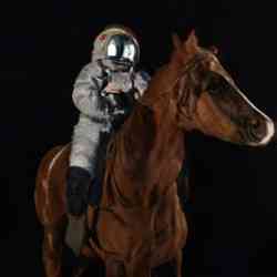
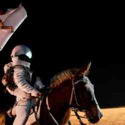
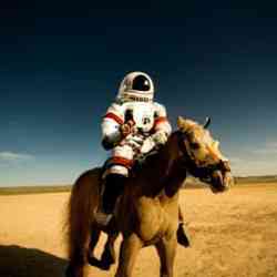
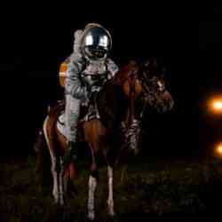
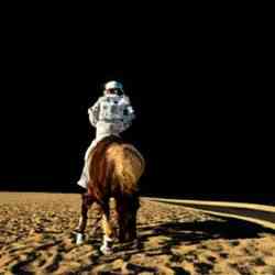
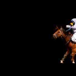
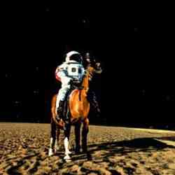
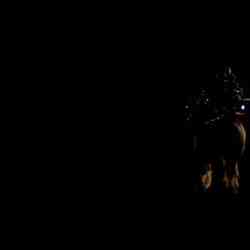
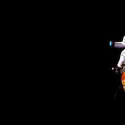
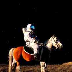
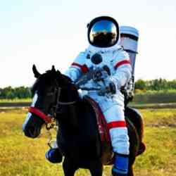
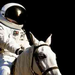
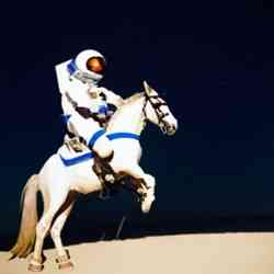
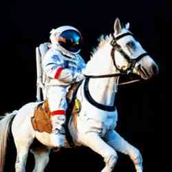
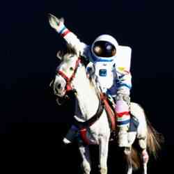
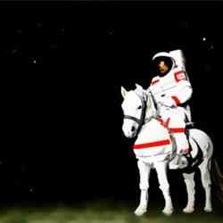
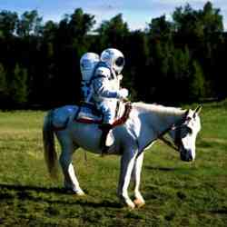
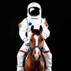
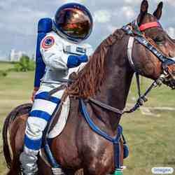
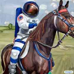
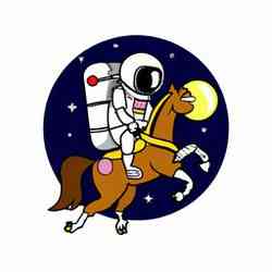
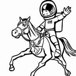
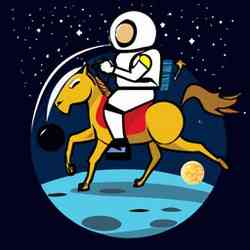
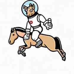
Conflicting	Ability to generate conflicting	“A horse riding an astronaut.”
	interactions b/w objects.	“A panda making latte art.”
DALL-E [53]	Subset of challenging prompts	“A triangular purple flower pot.”
	from [53].	“A cross-section view of a brain.”
Description	Ability to understand complex and long	“A small vessel propelled on water by oars, sails, or an engine.”
	text prompts describing objects.	“A mechanical or electrical device for measuring time.”
Marcus et al. [38]	Set of challenging prompts	“A pear cut into seven pieces arranged in a ring.”
	from [38].	“Paying for a quarter-sized pizza with a pizza-sized quarter.”
Misspellings	Ability to understand	“Rbefraigerator.”
	misspelled prompts.	“Tcennis rpacket.”
Positional	Ability to generate objects with	“A car on the left of a bus.”
	specified spatial positioning.	“A stop sign on the right of a refrigerator.”
Rare Words	Ability to understand rare words.	“Artophagous.”
		“Octothorpe.”
Reddit	Set of challenging prompts from	“A yellow and black bus cruising through the rainforest.”
	DALLE-2 Reddit.	“A medieval painting of the wifi not working.”
Text	Ability to generate quoted text.	“A storefront with ’Deep Learning’ written on it.”
		“A sign that says ’Text to Image’.”

Table A.1: Description and examples of the 11 categories in DrawBench.

Appendix D Imagen Detailed Abalations and Analysis

In this section, we perform ablations and provide a detailed analysis of Imagen.

D.1 Pre-trained Text Encoders

We explore several families of pre-trained text encoders: BERT [15], T5 [52], and CLIP [49]. There are several key differences between these encoders. BERT is trained on a smaller text-only corpus (approximately 20 GB, Wikipedia and BooksCorpus [84]) with a masking objective, and has relatively small model variants (upto 340M parameters). T5 is trained on a much larger C4 text-only corpus (approximately 800 GB) with a denoising objective, and has larger model variants (up to 11B parameters). The CLIP model is trained on an image-text corpus with an image-text contrastive objective. For T5 we use the encoder part for the contextual embeddings. For CLIP, we use the penultimate layer of the text encoder to get contextual embeddings. Note that we freeze the weights of these text encoders (i.e., we use off the shelf text encoders, without any fine-tuning on the text-to-image generation task). We explore a variety of model sizes for these text encoders.

We train a $64\times 64$, 300M parameter diffusion model, conditioned on the text embeddings generated from BERT (base, and large), T5 (small, base, large, XL, and XXL), and CLIP (ViT-L/14). We observe that scaling the size of the language model text encoders generally results in better image-text alignment as captured by the CLIP score as a function of number of training steps (see Fig. A.6). One can see that the best CLIP scores are obtained with the T5-XXL text encoder.

Since guidance weights are used to control image quality and text alignment, we also report ablation results using curves that show the trade-off between CLIP and FID scores as a function of the guidance weights (see Fig. 5(a)). We observe that larger variants of T5 encoder results in both better image-text alignment, and image fidelity. This emphasizes the effectiveness of large frozen text encoders for text-to-image models. Interestingly, we also observe that the T5-XXL encoder is on-par with the CLIP encoder when measured with CLIP and FID-10K on MS-COCO.

T5-XXL vs CLIP on DrawBench: We further compare T5-XXL and CLIP on DrawBench to perform a more comprehensive comparison of the abilities of these two text encoders. In our initial evaluations we observed that the 300M parameter models significantly underperformed on DrawBench. We believe this is primarily because DrawBench prompts are considerably more difficult than MS-COCO prompts.

In order to perform a meaningful comparison, we train 64$\times$64 1B parameter diffusion models with T5-XXL and CLIP text encoders for this evaluation. Fig. 5(b) shows the results. We find that raters are considerably more likely to prefer the generations from the model trained with the T5-XXL encoder over the CLIP text encoder, especially for image-text alignment. This indicates that language models are better than text encoders trained on image-text contrastive objectives in encoding complex and compositional text prompts. Fig. A.7 shows the category specific comparison between the two models. We observe that human raters prefer T5-XXL samples over CLIP samples in all 11 categories for image-text alignment demonstrating the effectiveness of large language models as text encoders for text to image generation.

(a) Pareto curves comparing various text encoders.

(b) Comparing T5-XXL and CLIP on DrawBench.

Figure A.5: Comparison between text encoders for text-to-image generation. For Fig. 5(a), we sweep over guidance values of $[1,1.25,1.5,1.75,2,3,4,5,6,7,8,9,10]$

Figure A.6: Training convergence comparison between text encoders for text-to-image generation.

(a) Alignment

(b) Fidelity

Figure A.7: T5-XXL vs. CLIP text encoder on DrawBench 7(a)) image-text alignment, and 7(b)) image fidelity.

D.2 Classifier-free Guidance and the Alignment-Fidelity Trade-off

Figure A.8: CLIP Score vs FID trade-off across various ${\widehat{𝐱}}_0$ thresholding methods for the 64$\times$64 model. We sweep over guidance values of $[1,1.25,1.5,1.75,2,3,4,5,6,7,8,9,10]$.

(a) No thresholding.

(b) Static thresholding.

(c) Dynamic thresholding.

Figure A.9: Thresholding techniques on $256\times 256$ samples for “A photo of an astronaut riding a horse.” Guidance weights increase from 1 to 5 as we go from top to bottom. No thresholding results in poor images with high guidance weights. Static thresholding is an improvement but still leads to oversaturated samples. Our dynamic thresholding leads to the highest quality images. See Fig. A.10 for more qualitative comparison.

(a) Samples using static thresholding.

(b) Samples using dynamic thresholding ($p=99.5$)

Figure A.10: Static vs. dynamic thresholding on non-cherry picked $256\times 256$ samples using a guidance weight of 5 for both the base model and the super-resolution model, using the same random seed. The text prompt used for these samples is “A photo of an astronaut riding a horse.” When using high guidance weights, static thresholding often leads to oversaturated samples, while our dynamic thresholding yields more natural looking images.

We observe that classifier-free guidance [27] is a key contributor to generating samples with strong image-text alignment, this is also consistent with the observations of [53, 54]. There is typically a trade-off between image fidelity and image-text alignment, as we iterate over the guidance weight. While previous work has typically used relatively small guidance weights, Imagen uses relatively large guidance weights for all three diffusion models. We found this to yield a good balance of sample quality and alignment. However, naive use of large guidance weights often produces relatively poor results. To enable the effective use of larger guidance we introduce several innovations, as described below.

Thresholding Techniques: First, we compare various thresholding methods used with classifier-free guidance. Fig. A.8 compares the CLIP vs. FID-10K score pareto frontiers for various thresholding methods of the base text-to-image $64\times 64$ model. We observe that our dynamic thresholding technique results in significantly better CLIP scores, and comparable or better FID scores than the static thresholding technique for a wide range of guidance weights. Fig. A.9 shows qualitative samples for thresholding techniques.

Guidance for Super-Resolution: We further analyze the impact of classifier-free guidance for our $64\times 64\to 256\times 256$ model. Fig. 11(a) shows the pareto frontiers for CLIP vs. FID-10K score for the $64\times 64\to 256\times 256$ super-resolution model. $\mathrm{aug}\mathrm{\_}\mathrm{level}$ specifies the level of noise augmentation applied to the input low-resolution image during inference ($\mathrm{aug}\mathrm{\_}\mathrm{level}=0$ means no noise). We observe that $\mathrm{aug}\mathrm{\_}\mathrm{level}=0$ gives the best FID score for all values of guidance weight. Furthermore, for all values of $\mathrm{aug}\mathrm{\_}\mathrm{level}$, we observe that FID improves considerably with increasing guidance weight upto around $7-10$. While generation using larger values of $\mathrm{aug}\mathrm{\_}\mathrm{level}$ gives slightly worse FID, it allows more varied range of CLIP scores, suggesting more diverse generations by the super-resolution model. In practice, for our best samples, we generally use $\mathrm{aug}\mathrm{\_}\mathrm{level}$ in $[0.1,0.3]$. Using large values of $\mathrm{aug}\mathrm{\_}\mathrm{level}$ and high guidance weights for the super-resolution models, Imagen can create different variations of a given $64\times 64$ image by altering the prompts to the super-resolution models (See Fig. A.12 for examples).

Impact of Conditioning Augmentation: Fig. 11(b) shows the impact of training super-resolution models with noise conditioning augmentation. Training with no noise augmentation generally results in worse CLIP and FID scores, suggesting noise conditioning augmentation is critical to attaining best sample quality similar to prior work [29]. Interestingly, the model trained without noise augmentation has much less variations in CLIP and FID scores across different guidance weights compared to the model trained with conditioning augmentation. We hypothesize that this is primarily because strong noise augmented training reduces the low-resolution image conditioning signal considerably, encouraging higher degree of dependence on conditioned text for the model.

(a) Comparison between different values of $\mathrm{aug}\mathrm{\_}\mathrm{level}$.

(b) Comparison between training with no noise augmentation “A” vs noise augmentation “B”

Figure A.11: CLIP vs FID-10K pareto curves showing the impact of noise augmentation on our $64\times 64\to 256\times 256$ model. For each study, we sweep over guidance values of $[1,3,5,7,8,10,12,15,18]$

Input	Unmodified	Oil Painting	Illustration

(a)

(b)

(c)

(d)

(e)

(f)

(g)

(h)

(i)

(j)

(k)

(l)

Figure A.12: Super-resolution variations for some $64\times 64$ generated images. We first generate the 64$\times$64 image using “A photo of … .”. Given generated $64\times 64$ images, we condition both the super-resolution models on different prompts in order to generate different upsampled variations. e.g. for oil painting we condition the super-resolution models on the prompt “An oil painting of … .”. Through a combination of large guidance weights and $\mathrm{aug}\mathrm{\_}\mathrm{level}=0.3$ for both super-res models we can generate different styles based on the style query through text.

D.3 Impact of Model Size

Fig. 13(b) plots the CLIP-FID score trade-off curves for various model sizes of the $64\times 64$ text-to-image U-Net model. We train each of the models with a batch size of 2048, and 400K training steps. As we scale from 300M parameters to 2B parameters for the U-Net model, we obtain better trade-off curves with increasing model capacity. Interestingly, scaling the frozen text encoder model size yields more improvement in model quality over scaling the U-Net model size. Scaling with a frozen text encoder is also easier since the text embeddings can be computed and stored offline during training.

D.3.1 Impact of Text Conditioning Schemas

We ablate various schemas for conditioning the frozen text embeddings in the base $64\times 64$ text-to-image diffusion model. Fig. 13(a) compares the CLIP-FID pareto curves for mean pooling, attention pooling, and cross attention. We find using any pooled embedding configuration (mean or attention pooling) performs noticeably worse compared to attending over the sequence of contextual embeddings in the attention layers. We implement the cross attention by concatenating the text embedding sequence to the key-value pairs of each self-attention layer in the base $64\times 64$ and $64\times 64\to 256\times 256$ models. For our $256\times 256\to 1024\times 1024$ model, since we have no self-attention layers, we simply added explicit cross-attention layers to attend over the text embeddings. We found this to improve both fidelity and image-text alignment with minimal computational costs.

(a) Comparison between different text encoders.

(b) Comparison between different model sizes.

Figure A.13: CLIP vs FID-10K pareto curves for different ablation studies for the base $64\times 64$ model. For each study, we sweep over guidance values of $[1,1.25,1.5,1.75,2,3,4,5,6,7,8,9,10]$

D.3.2 Comparison of U-Net vs Efficient U-Net

We compare the performance of U-Net with our new Efficient U-Net on the task of $64\times 64\to 256\times 256$ super-resolution task. Fig. A.14 compares the training convergence of the two architectures. We observe that Efficient U-Net converges significantly faster than U-Net, and obtains better performance overall. Our Efficient U-Net is also $\times 2-3$ faster at sampling.

Figure A.14: Comparison of convergence speed of U-Net vs Efficient U-Net on the $64\times 64\to 256\times 256$ super-resolution task.

Appendix E Comparison to GLIDE and DALL-E 2

Fig. A.15 shows category wise comparison between Imagen and DALL-E 2 [54] on DrawBench. We observe that human raters clearly prefer Imagen over DALL-E 2 in 7 out of 11 categories for text alignment. For sample fidelity, they prefer Imagen over DALL-E 2 in all 11 categories. Figures A.17, A.18, A.19, A.20 and A.21 show few qualitative comparisons between Imagen and DALL-E 2 samples used for this human evaluation study. Some of the categories where Imagen has a considerably larger preference over DALL-E 2 include Colors, Positional, Text, DALL-E and Descriptions. The authors in [54] identify some of these limitations of DALL-E 2, specifically they observe that DALLE-E 2 is worse than GLIDE [41] in binding attributes to objects such as colors, and producing coherent text from the input prompt (cf. the discussion of limitations in [54]). To this end, we also perform quantitative and qualitative comparison with GLIDE [41] on DrawBench. See Fig. A.16 for category wise human evaluation comparison between Imagen and GLIDE. See Figures A.22, A.23, A.24, A.25 and A.26 for qualitative comparisons. Imagen outperforms GLIDE on 8 out of 11 categories on image-text alignment, and 10 out of 11 categories on image fidelity. We observe that GLIDE is considerably better than DALL-E 2 in binding attributes to objects corroborating the observation by [54].

(a) Alignment

(b) Fidelity

Figure A.15: Imagen vs DALL-E 2 on DrawBench 15(a)) image-text alignment, and 15(b)) image fidelity.

(a) Alignment

(b) Fidelity

Figure A.16: Imagen vs GLIDE on DrawBench 16(a)) image-text alignment, and 16(b)) image fidelity.

Imagen (Ours)		DALL-E 2 [54]
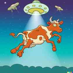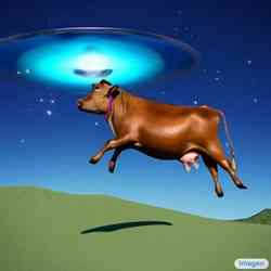
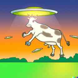
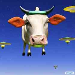
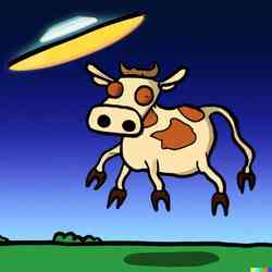
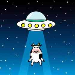
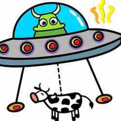
Hovering cow abducting aliens.
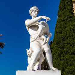
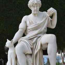
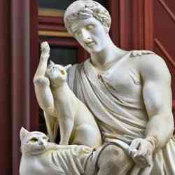
Greek statue of a man tripping over a cat.

Figure A.17: Example qualitative comparisons between Imagen and DALL-E 2 [54] on DrawBench prompts from Reddit category.

Imagen (Ours)		DALL-E 2 [54]
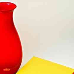
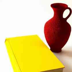
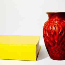
A yellow book and a red vase.
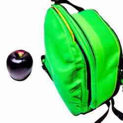
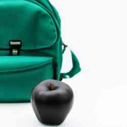
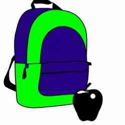
A black apple and a green backpack.

Figure A.18: Example qualitative comparisons between Imagen and DALL-E 2 [54] on DrawBench prompts from Colors category. We observe that DALL-E 2 generally struggles with correctly assigning the colors to the objects especially for prompts with more than one object.

Imagen (Ours)		DALL-E 2 [54]
A horse riding an astronaut.
A panda making latte art.

Figure A.19: Example qualitative comparisons between Imagen and DALL-E 2 [54] on DrawBench prompts from Conflicting category. We observe that both DALL-E 2 and Imagen struggle generating well aligned images for this category. However, Imagen often generates some well aligned samples, e.g. “A panda making latte art.”.

Imagen (Ours)		DALL-E 2 [54]
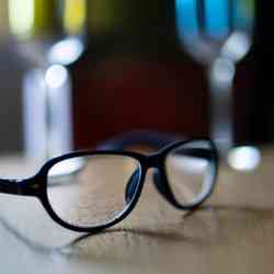
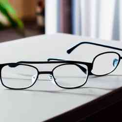
A couple of glasses are sitting on a table.
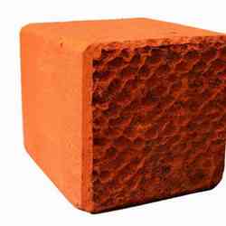
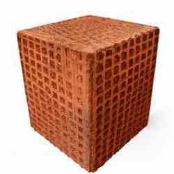
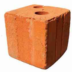
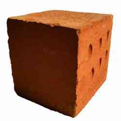
A cube made of brick. A cube with the texture of brick.

Figure A.20: Example qualitative comparisons between Imagen and DALL-E 2 [54] on DrawBench prompts from DALL-E category.

Imagen (Ours)		DALL-E 2 [54]
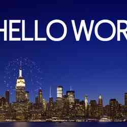
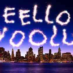
New York Skyline with Hello World written with fireworks on the sky.
A storefront with Text to Image written on it.

Figure A.21: Example qualitative comparisons between Imagen and DALL-E 2 [54] on DrawBench prompts from Text category. Imagen is significantly better than DALL-E 2 in prompts with quoted text.

Imagen (Ours)		GLIDE [41]
Hovering cow abducting aliens.
Greek statue of a man tripping over a cat.

Figure A.22: Example qualitative comparisons between Imagen and GLIDE [41] on DrawBench prompts from Reddit category.

Imagen (Ours)		GLIDE [41]
A yellow book and a red vase.
A black apple and a green backpack.

Figure A.23: Example qualitative comparisons between Imagen and GLIDE [41] on DrawBench prompts from Colors category. We observe that GLIDE is better than DALL-E 2 in assigning the colors to the objects.

Imagen (Ours)		GLIDE [41]
A horse riding an astronaut.
A panda making latte art.

Figure A.24: Example qualitative comparisons between Imagen and GLIDE [41] on DrawBench prompts from Conflicting category.

Imagen (Ours)		GLIDE [41]
A couple of glasses are sitting on a table.
A cube made of brick. A cube with the texture of brick.

Figure A.25: Example qualitative comparisons between Imagen and GLIDE [41] on DrawBench prompts from DALL-E category.

Imagen (Ours)		GLIDE [41]
New York Skyline with Hello World written with fireworks on the sky.
A storefront with Text to Image written on it.

Figure A.26: Example qualitative comparisons between Imagen and GLIDE [41] on DrawBench prompts from Text category. Imagen is significantly better than GLIDE too in prompts with quoted text.

Figure A.27: Efficient U-Net ResNetBlock. The ResNetBlock is used both by the DBlock and UBlock. Hyperparameter of the ResNetBlock is the number of channels channels: int.

Figure A.28: Efficient UNet DBlock. Hyperparameters of DBlock are: the stride of the block if there is downsampling stride: Optional[Tuple[int, int]], number of ResNetBlock per DBlock numResNetBlocksPerBlock: int, and number of channels channels: int. The dashed lined blocks are optional, e.g., not every DBlock needs to downsample or needs self-attention.

Figure A.29: Efficient U-Net UBlock. Hyperparameters of UBlock are: the stride of the block if there is upsampling stride: Optional[Tuple[int, int]], number of ResNetBlock per DBlock numResNetBlocksPerBlock: int, and number of channels channels: int. The dashed lined blocks are optional, e.g., not every UBlock needs to upsample or needs self-attention.

Figure A.30: Efficient U-Net architecture for ${64}^2\to {256}^2$.

def sample(): for t in reversed(range(T)): # Forward pass to get x0_t from z_t. x0_t = nn(z_t, t) # Static thresholding. x0_t = jnp.clip(x0_t, -1.0, 1.0) # Sampler step. z_tm1 = sampler_step(x0_t, z_t, t) z_t = z_tm1 return x0_t

(a) Implementation for static thresholding.

def sample(p: float): for t in reversed(range(T)): # Forward pass to get x0_t from z_t. x0_t = nn(z_t, t) # Dynamic thresholding (ours). s = jnp.percentile( jnp.abs(x0_t), p, axis=tuple(range(1, x0_t.ndim))) s = jnp.max(s, 1.0) x0_t = jnp.clip(x0_t, -s, s) / s # Sampler step. z_tm1 = sampler_step(x0_t, z_t, t) z_t = z_tm1 return x0_t

(b) Implementation for dynamic thresholding.

Figure A.31: Pseudo code implementation comparing static thresholding and dynamic thresholding.

def train_step( x_lr: jnp.ndarray, x_hr: jnp.ndarray): # Add augmentation to the low-resolution image. aug_level = jnp.random.uniform(0.0, 1.0) x_lr = apply_aug(x_lr, aug_level) # Diffusion forward process. t = jnp.random.uniform(0.0, 1.0) z_t = forward_process(x_hr, t) Optimize loss(x_hr, nn(z_t, x_lr, t, aug_level))

(a) Training using conditioning augmentation.

def sample(aug_level: float, x_lr: jnp.ndarray): # Add augmentation to the low-resolution image. x_lr = apply_aug(x_lr, aug_level) for t in reversed(range(T)): x_hr_t = nn(z_t, x_lr, t, aug_level) # Sampler step. z_tm1 = sampler_step(x_hr_t, z_t, t) z_t = z_tm1 return x_hr_t

(b) Sampling using conditioning augmentation.

Figure A.32: Pseudo-code implementation for training and sampling using conditioning augmentation. Text conditioning has not been shown for brevity.

Appendix F Implementation Details

F.1 $64\times 64$

Architecture: We adapt the architecture used in [16]. We use larger embed_dim for scaling up the architecture size. For conditioning on text, we use text cross attention at resolutions $[32,16,8]$ as well as attention pooled text embedding.

Optimizer: We use the Adafactor optimizer for training the base model. We use the default optax.adafactor parameters. We use a learning rate of 1e-4 with 10000 linear warmup steps.

Diffusion: We use the cosine noise schedule similar to [40]. We train using continuous time steps $t\sim 𝒰(0,1)$.

# 64 X 64 model. architecture = { "attn_resolutions": [32, 16, 8], "channel_mult": [1, 2, 3, 4], "dropout": 0, "embed_dim": 512, "num_res_blocks": 3, "per_head_channels": 64, "res_block_type": "biggan", "text_cross_attn_res": [32, 16, 8], "feature_pooling_type": "attention", "use_scale_shift_norm": True, } learning_rate = optax.warmup_cosine_decay_schedule( init_value=0.0, peak_value=1e-4, warmup_steps=10000, decay_steps=2500000, end_value=2500000) optimizer = optax.adafactor(lrs=learning_rate, weight_decay=0) diffusion_params = { "continuous_time": True, "schedule": { "name": "cosine", } }

F.2 $64\times 64\to 256\times 256$

Architecture: Below is the architecture specification for our $64\times 64\to 256\times 256$ super-resolution model. We use an Efficient U-Net architecture for this model.

Optimizer: We use the standard Adam optimizer with 1e-4 learning rate, and 10000 warmup steps.

Diffusion: We use the same cosine noise schedule as the base $64\times 64$ model. We train using continuous time steps $t\sim 𝒰(0,1)$.

architecture = { "dropout": 0.0, "feature_pooling_type": "attention", "use_scale_shift_norm": True, "blocks": [ { "channels": 128, "strides": (2, 2), "kernel_size": (3, 3), "num_res_blocks": 2, }, { "channels": 256, "strides": (2, 2), "kernel_size": (3, 3), "num_res_blocks": 4, }, { "channels": 512, "strides": (2, 2), "kernel_size": (3, 3), "num_res_blocks": 8, }, { "channels": 1024, "strides": (2, 2), "kernel_size": (3, 3), "num_res_blocks": 8, "self_attention": True, "text_cross_attention": True, "num_attention_heads": 8 } ] } learning_rate = optax.warmup_cosine_decay_schedule( init_value=0.0, peak_value=1e-4, warmup_steps=10000, decay_steps=2500000, end_value=2500000) optimizer = optax.adam( lrs=learning_rate, b1=0.9, b2=0.999, eps=1e-8, weight_decay=0) diffusion_params = { "continuous_time": True, "schedule": { "name": "cosine", } }

F.3 $256\times 256\to 1024\times 1024$

Architecture: Below is the architecture specification for our $256\times 256\to 1024\times 1024$ super-resolution model. We use the same configuration as the $64\times 64\to 256\times 256$ super-resolution model, except we do not use self-attention layers but rather have cross-attention layers (to the text embeddings).

Optimizer: We use the standard Adam optimizer with 1e-4 learning rate, and 10000 linear warmup steps.

Diffusion: We use the 1000 step linear noise schedule with start and end set to 1e-4 and 0.02 respectively. We train using continuous time steps $t\sim 𝒰(0,1)$.

"dropout": 0.0, "feature_pooling_type": "attention", "use_scale_shift_norm": true, "blocks"=[ { "channels": 128, "strides": (2, 2), "kernel_size": (3, 3), "num_res_blocks": 2, }, { "channels": 256, "strides": (2, 2), "kernel_size": (3, 3), "num_res_blocks": 4, }, { "channels": 512, "strides": (2, 2), "kernel_size": (3, 3), "num_res_blocks": 8, }, { "channels": 1024, "strides": (2, 2), "kernel_size": (3, 3), "num_res_blocks": 8, "text_cross_attention": True, "num_attention_heads": 8 } ]

References

- Aka et al. [2021] Osman Aka, Ken Burke, Alex Bauerle, Christina Greer, and Margaret Mitchell. Measuring Model Biases in the Absence of Ground Truth. In Proceedings of the 2021 AAAI/ACM Conference on AI, Ethics, and Society, 2021.
- Ba et al. [2016] Jimmy Lei Ba, Jamie Ryan Kiros, and Geoffrey E Hinton. Layer normalization. arXiv preprint arXiv:1607.06450, 2016.
-
Bender et al. [2021]
Emily M. Bender, Timnit Gebru, Angelina McMillan-Major, and Shmargaret
Shmitchell.
On the dangers of stochastic parrots: Can language models be too
big?
.
In Proceedings of FAccT 2021, 2021.
- Birhane et al. [2021] Abeba Birhane, Vinay Uday Prabhu, and Emmanuel Kahembwe. Multimodal datasets: misogyny, pornography, and malignant stereotypes. In arXiv:2110.01963, 2021.
- Bordia and Bowman [2017] Shikha Bordia and Samuel R. Bowman. Identifying and Reducing Gender Bias in Word-Level Language Models. In NAACL, 2017.
- Brock et al. [2018] Andrew Brock, Jeff Donahue, and Karen Simonyan. Large scale gan training for high fidelity natural image synthesis. arXiv preprint arXiv:1809.11096, 2018.
- Brown et al. [2020] Tom B. Brown, Benjamin Mann, Nick Ryder, Melanie Subbiah, Jared Kaplan, Prafulla Dhariwal, Arvind Neelakantan, Pranav Shyam, Girish Sastry, Amanda Askell, Sandhini Agarwal, Ariel Herbert-Voss, Gretchen Krueger, Tom Henighan, Rewon Child, Aditya Ramesh, Daniel M. Ziegler, Jeffrey Wu, Clemens Winter, Christopher Hesse, Mark Chen, Eric Sigler, Mateusz Litwin, Scott Gray, Benjamin Chess, Jack Clark, Christopher Berner, Sam McCandlish, Alec Radford, Ilya Sutskever, and Dario Amodei. Language Models are Few-Shot Learners. In NeurIPS, 2020.
- Buolamwini and Gebru [2018] Joy Buolamwini and Timnit Gebru. Gender shades: Intersectional accuracy disparities in commercial gender classification. In Conference on Fairness, Accountability and Transparency, FAT 2018, 23-24 February 2018, New York, NY, USA, Proceedings of Machine Learning Research. PMLR, 2018.
- Burns et al. [2018] Kaylee Burns, Lisa Hendricks, Trevor Darrell, and Anna Rohrbach. Women also snowboard: Overcoming bias in captioning models. In European Conference on Computer Vision (ECCV), 2018.
- Cho et al. [2022] Jaemin Cho, Abhay Zala, and Mohit Bansal. Dall-eval: Probing the reasoning skills and social biases of text-to-image generative transformers. arxiv:2202.04053, 2022.
- Chowdhery et al. [2022] Aakanksha Chowdhery, Sharan Narang, Jacob Devlin, Maarten Bosma, Gaurav Mishra, Adam Roberts, Paul Barham, Hyung Won Chung, Charles Sutton, Sebastian Gehrmann, Parker Schuh, Kensen Shi, Sasha Tsvyashchenko, Joshua Maynez, Abhishek Rao, Parker Barnes, Yi Tay, Noam Shazeer, Vinodkumar Prabhakaran, Emily Reif, Nan Du, Ben Hutchinson, Reiner Pope, James Bradbury, Jacob Austin, Michael Isard, Guy Gur-Ari, Pengcheng Yin, Toju Duke, Anselm Levskaya, Sanjay Ghemawat, Sunipa Dev, Henryk Michalewski, Xavier Garcia, Vedant Misra, Kevin Robinson, Liam Fedus, Denny Zhou, Daphne Ippolito, David Luan, Hyeontaek Lim, Barret Zoph, Alexander Spiridonov, Ryan Sepassi, David Dohan, Shivani Agrawal, Mark Omernick, Andrew M. Dai, Thanumalayan Sankaranarayana Pillai, Marie Pellat, Aitor Lewkowycz, Erica Moreira, Rewon Child, Oleksandr Polozov, Katherine Lee, Zongwei Zhou, Xuezhi Wang, Brennan Saeta, Mark Diaz, Orhan Firat, Michele Catasta, Jason Wei, Kathy Meier-Hellstern, Douglas Eck, Jeff Dean, Slav Petrov, and Noah Fiedel. PaLM: Scaling Language Modeling with Pathways. In arXiv:2001.08361, 2022.
- Crowson et al. [2022] Katherine Crowson, Stella Biderman, Daniel Kornis, Dashiell Stander, Eric Hallahan, Louis Castricato, and Edward Raff. Vqgan-clip: Open domain image generation and editing with natural language guidance. arXiv preprint arXiv:2204.08583, 2022.
- De Bortoli et al. [2021] Valentin De Bortoli, James Thornton, Jeremy Heng, and Arnaud Doucet. Diffusion schrödinger bridge with applications to score-based generative modeling. Advances in Neural Information Processing Systems, 34, 2021.
- Denton et al. [2015] Emily Denton, Soumith Chintala, Arthur Szlam, and Rob Fergus. Deep Generative Image Models using a Laplacian Pyramid of Adversarial Networks. In NIPS, 2015.
- Devlin et al. [2019] Jacob Devlin, Ming-Wei Chang, Kenton Lee, and Kristina Toutanova. BERT: Pre-training of Deep Bidirectional Transformers for Language Understanding. In NAACL, 2019.
- Dhariwal and Nichol [2022] Prafulla Dhariwal and Alex Nichol. Diffusion models beat gans on image synthesis. In NeurIPS, 2022.
- Ding et al. [2021] Ming Ding, Zhuoyi Yang, Wenyi Hong, Wendi Zheng, Chang Zhou, Da Yin, Junyang Lin, Xu Zou, Zhou Shao, Hongxia Yang, et al. Cogview: Mastering text-to-image generation via transformers. Advances in Neural Information Processing Systems, 34, 2021.
- Dulhanty, Chris [2020] Dulhanty, Chris. Issues in Computer Vision Data Collection: Bias, Consent, and Label Taxonomy. In UWSpace, 2020.
- Esser et al. [2021] Patrick Esser, Robin Rombach, and Bjorn Ommer. Taming transformers for high-resolution image synthesis. In Proceedings of the IEEE/CVF Conference on Computer Vision and Pattern Recognition, pages 12873–12883, 2021.
- Franks and Waldman [2019] Mary Anne Franks and Ari Ezra Waldman. Sex, lies and videotape: deep fakes and free speech delusions. Maryland Law Review, 78(4):892–898, 2019.
- Fu et al. [2021] Tsu-Jui Fu, Xin Eric Wang, and William Yang Wang. Language-Driven Image Style Transfer. arXiv preprint arXiv:2106.00178, 2021.
- Gafni et al. [2022] Oran Gafni, Adam Polyak, Oron Ashual, Shelly Sheynin, Devi Parikh, and Yaniv Taigman. Make-a-scene: Scene-based text-to-image generation with human priors. arXiv preprint arXiv:2203.13131, 2022.
- Gebru et al. [2020] Timnit Gebru, Jamie Morgenstern, Briana Vecchione, Jennifer Wortman Vaughan, Hanna Wallach, Hal Daumé III, and Kate Crawford. Datasheets for Datasets. arXiv:1803.09010 [cs], March 2020.
- Harvey and LaPlace [2019] Adam Harvey and Jules LaPlace. MegaPixels: Origins and endpoints of biometric datasets "In the Wild". https://megapixels.cc, 2019.
- Hessel et al. [2021] Jack Hessel, Ari Holtzman, Maxwell Forbes, Ronan Le Bras, and Yejin Choi. Clipscore: A reference-free evaluation metric for image captioning. arXiv preprint arXiv:2104.08718, 2021.
- Heusel et al. [2017] Martin Heusel, Hubert Ramsauer, Thomas Unterthiner, Bernhard Nessler, and Sepp Hochreiter. Gans trained by a two time-scale update rule converge to a local nash equilibrium. arXiv preprint arXiv:1706.08500, 2017.
- Ho and Salimans [2021] Jonathan Ho and Tim Salimans. Classifier-free diffusion guidance. In NeurIPS 2021 Workshop on Deep Generative Models and Downstream Applications, 2021.
- Ho et al. [2020] Jonathan Ho, Ajay Jain, and Pieter Abbeel. Denoising Diffusion Probabilistic Models. NeurIPS, 2020.
- Ho et al. [2022] Jonathan Ho, Chitwan Saharia, William Chan, David J Fleet, Mohammad Norouzi, and Tim Salimans. Cascaded diffusion models for high fidelity image generation. JMLR, 2022.
- Hughes et al. [2021] Rowan T. Hughes, Liming Zhu, and Tomasz Bednarz. Generative adversarial networks-enabled human-artificial intelligence collaborative applications for creative and design industries: A systematic review of current approaches and trends. Frontiers in artificial intelligence, 4, 2021.
- Jia et al. [2021] Chao Jia, Yinfei Yang, Ye Xia, Yi-Ting Chen, Zarana Parekh, Hieu Pham, Quoc Le, Yun-Hsuan Sung, Zhen Li, and Tom Duerig. Scaling up visual and vision-language representation learning with noisy text supervision. In International Conference on Machine Learning, pages 4904–4916. PMLR, 2021.
- Kadkhodaie and Simoncelli [2020] Zahra Kadkhodaie and Eero P Simoncelli. Solving linear inverse problems using the prior implicit in a denoiser. arXiv preprint arXiv:2007.13640, 2020.
- Kadkhodaie and Simoncelli [2021] Zahra Kadkhodaie and Eero P Simoncelli. Stochastic solutions for linear inverse problems using the prior implicit in a denoiser. Advances in Neural Information Processing Systems, 34, 2021.
- Kim and Ye [2021] Gwanghyun Kim and Jong Chul Ye. Diffusionclip: Text-guided image manipulation using diffusion models. arXiv preprint arXiv:2110.02711, 2021.
- Kingma et al. [2021] Diederik P Kingma, Tim Salimans, Ben Poole, and Jonathan Ho. Variational diffusion models. arXiv preprint arXiv:2107.00630, 2021.
- Lin et al. [2014] Tsung-Yi Lin, Michael Maire, Serge Belongie, Lubomir Bourdev, Ross Girshick, James Hays, Pietro Perona, Deva Ramanan, Lawrence Zitnick, and Piotr Dollár. Microsoft COCO: Common Objects in Context. In ECCV, 2014.
- Mansimov et al. [2016] Elman Mansimov, Emilio Parisotto, Jimmy Lei Ba, and Ruslan Salakhutdinov. Generating Images from Captions with Attention. In ICLR, 2016.
- Marcus et al. [2022] Gary Marcus, Ernest Davis, and Scott Aaronson. A very preliminary analysis of DALL-E 2. In arXiv:2204.13807, 2022.
- Menick and Kalchbrenner [2019] Jacob Menick and Nal Kalchbrenner. Generating High Fidelity Images with Subscale Pixel Networks and Multidimensional Upscaling. In ICLR, 2019.
- Nichol and Dhariwal [2021] Alex Nichol and Prafulla Dhariwal. Improved denoising diffusion probabilistic models. arXiv preprint arXiv:2102.09672, 2021.
- Nichol et al. [2021] Alex Nichol, Prafulla Dhariwal, Aditya Ramesh, Pranav Shyam, Bob McGrew Pamela Mishkin, Ilya Sutskever, and Mark Chen. GLIDE: Towards Photorealistic Image Generation and Editing with Text-Guided Diffusion Models. In arXiv:2112.10741, 2021.
- Parmar et al. [2022] Gaurav Parmar, Richard Zhang, and Jun-Yan Zhu. On Aliased Resizing and Surprising Subtleties in GAN Evaluation. In CVPR, 2022.
- Paullada et al. [2021] Amandalynne Paullada, Inioluwa Deborah Raji, Emily M. Bender, Emily Denton, and Alex Hanna. Data and its (dis)contents: A survey of dataset development and use in machine learning research. Patterns, 2(11):100336, 2021.
- Prabhu and Birhane [2020] Vinay Uday Prabhu and Abeba Birhane. Large image datasets: A pyrrhic win for computer vision? arXiv:2006.16923, 2020.
- Pushkarna et al. [2022] Mahima Pushkarna, Andrew Zaldivar, and Oddur Kjartansson. Data cards: Purposeful and transparent dataset documentation for responsible ai. In Proceedings of the 2021 ACM Conference on Fairness, Accountability, and Transparency, 2022.
- Radford et al. [2017] Alec Radford, Rafal Jozefowicz, and Ilya Sutskever. Learning to Generate Reviews and Discovering Sentiment. In arXiv:1704.01444, 2017.
- Radford et al. [2018] Alec Radford, Karthik Narasimhan, Tim Salimans, and Ilya Sutskever. Improving Language Understanding by Generative Pre-Training. In preprint, 2018.
- Radford et al. [2019] Alec Radford, Jeffrey Wu, Rewon Child, David Luan, Dario Amodei, and Ilya Sutskever. Language Models are Unsupervised Multitask Learners. In preprint, 2019.
- Radford et al. [2021] Alec Radford, Jong Wook Kim, Chris Hallacy, Aditya Ramesh, Gabriel Goh, Sandhini Agarwal, Girish Sastry, Amanda Askell, Pamela Mishkin, Jack Clark, Gretchen Krueger, and Ilya Sutskever. Learning Transferable Visual Models From Natural Language Supervision. In ICML, 2021.
- Rae et al. [2021] Jack Rae, Sebastian Borgeaud, Trevor Cai, Katie Millican, Jordan Hoffmann, Francis Song, John Aslanides, Sarah Henderson, Roman Ring, Susannah Young, Eliza Rutherford, Tom Hennigan, Jacob Menick, Albin Cassirer, Richard Powell, George Driessche, Lisa Hendricks, Maribeth Rauh, Po-Sen Huang, and Geoffrey Irving. Scaling language models: Methods, analysis & insights from training gopher. arXiv:2112.11446, 2021.
- Raffel et al. [2017] Colin Raffel, Minh-Thang Luong, Peter J. Liu, Ron J. Weiss, and Douglas Eck. Online and Linear-Time Attention by Enforcing Monotonic Alignments. In ICML, 2017.
- Raffel et al. [2020] Colin Raffel, Noam Shazeer, Adam Roberts, Katherine Lee, Sharan Narang, Michael Matena, Yanqi Zhou, Wei Li, and Peter J. Liu. Exploring the Limits of Transfer Learning with a Unified Text-to-Text Transformer. JMLR, 21(140), 2020.
- Ramesh et al. [2021] Aditya Ramesh, Mikhail Pavlov, Gabriel Goh, Scott Gray, Chelsea Voss, Alec Radford, Mark Chen, and Ilya Sutskever. Zero-Shot Text-to-Image Generation. In ICML, 2021.
- Ramesh et al. [2022] Aditya Ramesh, Prafulla Dhariwal, Alex Nichol, Casey Chu, and Mark Chen. Hierarchical Text-Conditional Image Generation with CLIP Latents. In arXiv, 2022.
- Razavi et al. [2019] Ali Razavi, Aaron van den Oord, and Oriol Vinyals. Generating diverse high-fidelity images with vq-vae-2. arXiv preprint arXiv:1906.00446, 2019.
- Reed et al. [2016] Scott Reed, Zeynep Akata, Xinchen Yan, Lajanugen Logeswaran, Bernt Schiele, and Honglak Lee. Generative adversarial text to image synthesis. In International conference on machine learning, pages 1060–1069. PMLR, 2016.
- Rombach et al. [2022] Robin Rombach, Andreas Blattmann, Dominik Lorenz, Patrick Esser, and Björn Ommer. High-Resolution Image Synthesis with Latent Diffusion Models. In CVPR, 2022.
- Saharia et al. [2021a] Chitwan Saharia, William Chan, Huiwen Chang, Chris A. Lee, Jonathan Ho, Tim Salimans, David J. Fleet, and Mohammad Norouzi. Palette: Image-to-Image Diffusion Models. In arXiv:2111.05826, 2021a.
- Saharia et al. [2021b] Chitwan Saharia, Jonathan Ho, William Chan, Tim Salimans, David J Fleet, and Mohammad Norouzi. Image super-resolution via iterative refinement. arXiv preprint arXiv:2104.07636, 2021b.
- Scheuerman et al. [2021] Morgan Klaus Scheuerman, Emily L. Denton, and A. Hanna. Do datasets have politics? disciplinary values in computer vision dataset development. Proceedings of the ACM on Human-Computer Interaction, 5:1 – 37, 2021.
- Schuhmann et al. [2021] Christoph Schuhmann, Richard Vencu, Romain Beaumont, Robert Kaczmarczyk, Clayton Mullis, Aarush Katta, Theo Coombes, Jenia Jitsev, and Aran Komatsuzaki. Laion-400m: Open dataset of clip-filtered 400 million image-text pairs. arXiv preprint arXiv:2111.02114, 2021.
- Sequeira et al. [2021] Lucas Sequeira, Bruno Moreschi, Amanda Jurno, and Vinicius Arruda dos Santos. Which faces can AI generate? Normativity, whiteness and lack of diversity in This Person Does Not Exist. In CVPR Workshop Beyond Fairness: Towards a Just, Equitable, and Accountable Computer Vision, 2021.
- Sohl-Dickstein et al. [2015] Jascha Sohl-Dickstein, Eric Weiss, Niru Maheswaranathan, and Surya Ganguli. Deep unsupervised learning using nonequilibrium thermodynamics. In International Conference on Machine Learning, pages 2256–2265. PMLR, 2015.
- Song et al. [2020] Jiaming Song, Chenlin Meng, and Stefano Ermon. Denoising diffusion implicit models. arXiv preprint arXiv:2010.02502, 2020.
- Song and Ermon [2019] Yang Song and Stefano Ermon. Generative Modeling by Estimating Gradients of the Data Distribution. NeurIPS, 2019.
- Song et al. [2021] Yang Song, Jascha Sohl-Dickstein, Diederik P Kingma, Abhishek Kumar, Stefano Ermon, and Ben Poole. Score-based generative modeling through stochastic differential equations. In ICLR, 2021.
- Srinivasan and Uchino [2021] Ramya Srinivasan and Kanji Uchino. Biases in generative art: A causal look from the lens of art history. In Proceedings of the 2021 ACM Conference on Fairness, Accountability, and Transparency, page 41–51, 2021.
- Steed and Caliskan [2021] Ryan Steed and Aylin Caliskan. Image representations learned with unsupervised pre-training contain human-like biases. In Proceedings of the 2021 ACM Conference on Fairness, Accountability, and Transparency, FAccT ’21, page 701–713. Association for Computing Machinery, 2021.
- Tao et al. [2020] Ming Tao, Hao Tang, Songsong Wu, Nicu Sebe, Xiao-Yuan Jing, Fei Wu, and Bingkun Bao. Df-gan: Deep fusion generative adversarial networks for text-to-image synthesis. arXiv preprint arXiv:2008.05865, 2020.
- Tzen and Raginsky [2019] Belinda Tzen and Maxim Raginsky. Neural Stochastic Differential Equations: Deep Latent Gaussian Models in the Diffusion Limit. In arXiv:1905.09883, 2019.
- Van Den Oord et al. [2017] Aaron Van Den Oord, Oriol Vinyals, et al. Neural discrete representation learning. Advances in neural information processing systems, 30, 2017.
- Vincent [2011] Pascal Vincent. A connection between score matching and denoising autoencoders. Neural Computation, 23(7):1661–1674, 2011.
- Wang et al. [2018] Ting-Chun Wang, Ming-Yu Liu, Jun-Yan Zhu, Andrew Tao, Jan Kautz, and Bryan Catanzaro. High-resolution image synthesis and semantic manipulation with conditional gans. In Proceedings of the IEEE conference on computer vision and pattern recognition, pages 8798–8807, 2018.
- Weston et al. [2011] Jason Weston, Samy Bengio, and Nicolas Usunier. Wsabie: Scaling up to large vocabulary image annotation. In Twenty-Second International Joint Conference on Artificial Intelligence, 2011.
- Whang et al. [2021] Jay Whang, Mauricio Delbracio, Hossein Talebi, Chitwan Saharia, Alexandros G Dimakis, and Peyman Milanfar. Deblurring via stochastic refinement. arXiv preprint arXiv:2112.02475, 2021.
- Xu et al. [2018a] Tao Xu, Pengchuan Zhang, Qiuyuan Huang, Han Zhang, Zhe Gan, Xiaolei Huang, and Xiaodong He. AttnGAN: Fine-Grained Text to Image Generation with Attentional Generative Adversarial Networks. In CVPR, 2018a.
- Xu et al. [2018b] Tao Xu, Pengchuan Zhang, Qiuyuan Huang, Han Zhang, Zhe Gan, Xiaolei Huang, and Xiaodong He. Attngan: Fine-grained text to image generation with attentional generative adversarial networks. In Proceedings of the IEEE conference on computer vision and pattern recognition, pages 1316–1324, 2018b.
- Ye et al. [2021] Hui Ye, Xiulong Yang, Martin Takac, Rajshekhar Sunderraman, and Shihao Ji. Improving text-to-image synthesis using contrastive learning. arXiv preprint arXiv:2107.02423, 2021.
- Yu et al. [2021] Jiahui Yu, Xin Li, Jing Yu Koh, Han Zhang, Ruoming Pang, James Qin, Alexander Ku, Yuanzhong Xu, Jason Baldridge, and Yonghui Wu. Vector-quantized image modeling with improved vqgan. arXiv preprint arXiv:2110.04627, 2021.
- Yu et al. [2022] Jiahui Yu, Zirui Wang, Vijay Vasudevan, Legg Yeung, Mojtaba Seyedhosseini, and Yonghui Wu. Coca: Contrastive captioners are image-text foundation models. arXiv preprint arXiv:2205.01917, 2022.
- Zhang et al. [2021] Han Zhang, Jing Yu Koh, Jason Baldridge, Honglak Lee, and Yinfei Yang. Cross-Modal Contrastive Learning for Text-to-Image Generation. In CVPR, 2021.
- Zhou et al. [2021] Yufan Zhou, Ruiyi Zhang, Changyou Chen, Chunyuan Li, Chris Tensmeyer, Tong Yu, Jiuxiang Gu, Jinhui Xu, and Tong Sun. Lafite: Towards language-free training for text-to-image generation. arXiv preprint arXiv:2111.13792, 2021.
- Zhu et al. [2019] Minfeng Zhu, Pingbo Pan, Wei Chen, and Yi Yang. Dm-gan: Dynamic memory generative adversarial networks for text-to-image synthesis. In Proceedings of the IEEE/CVF Conference on Computer Vision and Pattern Recognition, pages 5802–5810, 2019.
- Zhu et al. [2015] Yukun Zhu, Ryan Kiros, Rich Zemel, Ruslan Salakhutdinov, Raquel Urtasun, Antonio Torralba, and Sanja Fidler. Aligning books and movies: Towards story-like visual explanations by watching movies and reading books. In ICCV, 2015.