使用 Wi-Fi 进行无线传感实践：教程

Zheng Yang hmilyyz@gmail.com Tsinghua UniversityBeijingChina , Yi Zhang zhangyithss@gmail.com Tsinghua UniversityBeijingChina , Guoxuan Chi chiguoxuan@gmail.com Tsinghua UniversityBeijingChina and Guidong Zhang zhanggd18@gmail.com Tsinghua UniversityBeijingChina

摘要。

随着无线通信技术的快速发展，无线接入点（AP）和物联网（IoT）设备已在我们的周围广泛部署。各种类型的无线信号（例如 Wi-Fi、LoRa、LTE）正在充斥着我们的生活和工作空间。先前的研究揭示了无线电波在传播过程中受到空间结构的调制（例如反射、衍射和散射）并叠加在接收器上的事实。这种观察使我们能够根据接收到的无线信号重建周围环境，称为“无线传感”。无线传感是一项新兴技术，可实现广泛的应用，例如用于人机交互的手势识别、用于医疗保健的生命体征监测以及用于安全管理的入侵检测。与其他传感范例（例如基于视觉和基于IMU的传感）相比，无线传感解决方案具有独特的优势，例如高覆盖率、普遍性、低成本以及在不利光线和纹理场景下的鲁棒性。此外，无线传感解决方案在计算开销和设备尺寸方面通常都是轻量级的。本教程以 Wi-Fi 传感为例。既介绍了理论原理，又介绍了代码实现 ¹¹1代码和数据可在http://tns.thss.tsinghua.edu.cn/wst和http获取： //tns.thss.tsinghua.edu.cn/widar3.0。数据收集、信号处理、特征提取和模型设计。此外，本教程还重点介绍了最先进的深度学习模型（例如 CNN、RNN 和对抗性学习模型）及其在无线传感系统中的应用。我们希望本教程能够帮助其他研究领域的人们进入无线传感研究，更多地了解其理论、设计和实现技巧，促进无线传感研究领域的繁荣。

1. 无线传感背景

1.1. 什么是无线传感

各种传感器和传感器网络彻底扩展了人类对物理世界的感知。如今，已经部署了大量的传感器来完成各种传感任务，导致了巨大的部署和维护开销。当需要大传感规模时，这个问题变得越来越麻烦。以室内行人跟踪为例，专门的跟踪系统仅覆盖房间级别的区域，与人日常生活中的移动区域相比太小。需要多个跟踪系统来实现现实生活环境（例如房屋、校园、市场、机场和办公室）的实际传感覆盖，并且成本不可避免地增加。

考虑到传感器的成本限制，许多先驱者在过去十年中试图找出替代解决方案。如今，各种类型的信号（例如 Wi-Fi、LoRa、LTE）正在填充我们的生活和工作空间进行无线通信，可以利用这些信号来捕获环境变化，而不会造成额外的开销。根据电磁学理论，发射机（Tx）发出的无线电信号在传播过程中会经历反射、衍射、散射等各种物理现象，形成多条传播路径。这样，接收机采集到的叠加多径信号就携带了信号传播环境的空间信息。无线传感仅依赖于周围的无线信号和无处不在的通信设备，成为环境传感的一种新颖范式。

近年来，无线传感技术吸引了许多研究兴趣，通过提高传感粒度、提高系统鲁棒性和探索应用场景，将无线传感从想象变为现实。他们在无线传感方面的许多著作已发表在旗舰会议和期刊上，例如 ACM SIGCOMM、ACM MobiCom、ACM MobiSys、IEEE INFOCOM、USENIX NSDI、IEEE/ACM ToN、IEEE JSAC 和 IEEE TMC。此外，不少知名企业也在探索无传感器传感的产品化，推出各种用于人机交互、安防监控、医疗保健等的物联网设备。

1.2. 无线传感与计算机视觉的比较

典型的射频信号 (300 kHz - 300 GHz) 和可见光信号 (380 THz - 750 THz) 本质上是电磁 (EM) 波。当电磁波在我们的物理世界中传播时，会经历各种物理现象，例如反射、衍射和散射。多径信号最终叠加并被接收机接收。因此，接收到的叠加信号携带了信号传播空间的物理信息。

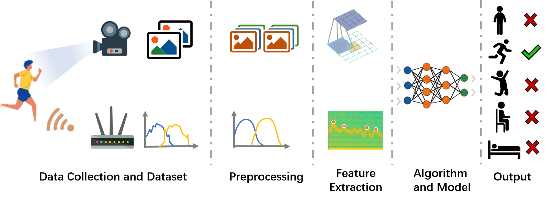
基于射频和基于视觉的传感算法都具有相似的过程。他们首先对接收到的信号（天线处的无线电信号或相机镜头处的可见光）进行分析，从中提取反映传播空间的特征，最后通过算法进行解析，从而实现对周围环境的感知。

与基于视觉的传感相比，无线传感解决方案具有独特的优势，例如高覆盖率（Chi等人，2021）、普遍性、低成本以及在不利光线和纹理场景下的鲁棒性（Chi等人，2021）。等人，2022）。

Refer to caption — 图1。基于视觉的传感和基于射频的传感过程的比较。

1.3. 无线传感应用

无线传感系统能够感知周围环境、物体和人体的变化。在本小节中，我们以被动人体感应应用程序为例，它是指以人为中心的感应应用程序，不需要用户携带任何设备。因此，这种传感应用也被称为无设备传感或非侵入式传感。被动人体感应可实现广泛的应用，包括智能家居、安全监控和医疗保健。

在智能家居应用中，被动人体感应根据用户的物理位置、手势和姿势来识别人的行为或意图。被动人体感应带来更好的用户体验，而不会对用户施加限制。例如，用户只需在空中做出手势就可以远程控制电视、电脑或洗衣机等电器设备（Zheng等人，2019；Abdelnasser等人，2015）。同样，在玩视频游戏时，用户可以通过执行不同的姿势来与计算机进行交互（Jiang等人，2020）。

在安全监控应用中，传统方法采用红外或RGB摄像机来监控非法入侵、保护贵重财产和处理紧急情况。然而，摄像机受到有限视野或不透明或金属物体遮挡的限制，当目标不在监控摄像机的视距 (LoS) 区域或隐藏在其他物体后面时，这些方法就会失败。与视觉监控相比，无线传感技术利用无线电信号，提供无线设备周围的全向覆盖，并且不易出现堵塞。例如，无线信号可用于检测非法入侵（吴等人，2015；钱等人，2014）。此外，它们还可以用于检测财产是否已从原来的位置移动。

在医疗保健应用中，可以利用被动人体传感来检测人体呼吸、心跳、步态和意外跌倒等生命信号。具体来说，一些研究人员利用 Wi-Fi 信号来检测人体呼吸（Wang 等人，2016）以进行睡眠监测。其他一些作品（Zhang 等人，2020；Wu 等人，2020）从 Wi-Fi 信号中提取步态模式来识别人类身份。最近，Wi-Fi 信号被进一步用于检测意外跌倒，以减轻对可穿戴传感器的需求（Hu 等人，2020；Palipana 等人，2019）。

2. 了解CSI

信道状态信息 (CSI) 为大多数无线传感技术奠定了基础，包括 Wi-Fi 传感、LTE 传感等。 CSI 提供子载波级粒度的物理信道测量，并且可以从商用 Wi-Fi 网络接口控制器 (NIC) 轻松访问。

CSI描述了无线信号的传播过程，因此包含了传播空间的几何信息。因此，理解CSI与空间几何参数之间的映射关系为特征提取和感知算法设计奠定了基础。

本节重点介绍两种主流的 CSI 模型：光线追踪模型和散射模型。这两个模型基于理解信号传播过程的两个视角。因此，它们具有独特的优势，适用于不同的场景。

2.1. 光线追踪模型

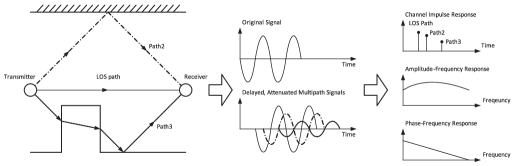
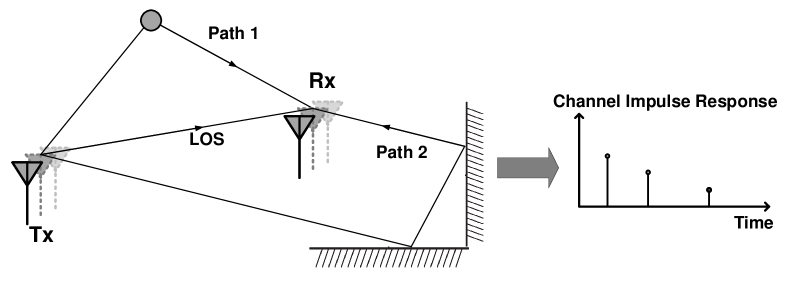
在典型的室内环境中，由于无线电波的反射，发射器发送的信号通过多条路径到达接收器。沿着每条路径，信号都会经历一定的衰减和相移。接收到的信号是发送信号的多个混叠版本的叠加。因此，接收端在特定时刻测得的复基带信号强度可写为（Yang等人，2013）：

(1)

V=\sum_{n=1}^{N}{\lVert V_{n}\rVert e^{-j\phi_{n}}},

其中 $V_{n}$ 和 $\phi_{n}$ 是 $n^{th}$ 多径分量的幅度和相位（注意隐式考虑了信号的调制方案）， $N$ 是组件总数。在此基础上，接收信号强度指标（RSSI）可以写成以分贝（dB）为单位的接收功率：

(2)

\mathrm{RSSI}=10\log_{2}\left(\lVert V\rVert^{2}\right).

由于多径分量的叠加，RSSI不仅随着传播距离以信号波长量级变化而快速变化，而且会随着时间的推移而波动，即使对于静态链路也是如此。特定多径分量的微小变化可能会导致显着的建设性或破坏性多径分量，从而导致 RSSI 出现相当大的波动。

RSSI的本质缺点是不能反映多径效应。无线信道被建模为线性时间滤波器，以充分表征各个路径，称为信道脉冲响应 (CIR)。在时不变假设下，CIR $h(t)$ 表示为：

(3)

h(t)=\sum_{n=1}^{N}{\alpha_{n}e^{-j\phi_{n}}\delta(t-\tau_{n})},

其中 $\alpha_{n}$ 、 $\phi_{n}$ 和 $\tau_{n}$ 分别是 $n^{th}$ 路径的复衰减、相位和时间延迟。 $N$ 是多径总数， $\delta(\cdot)$ 是Dirac delta函数。每个脉冲代表一个延迟的多径分量，乘以相应的幅度和相位。

在频域，多径引起频率选择性衰落，其特征是信道频率响应（CFR）。 CFR本质上是CIR的傅立叶变换。它由幅度响应和相位响应组成。图2演示了多径场景、发送信号、接收信号以及示例性信道响应。 CIR 和 CFR 都描述了小规模多径效应，用于细粒度信道测量。请注意，CIR 和 CFR 涉及复振幅和衰减，而信号功率方面的另一对参数是功率延迟分布 (PDP) 和功率谱密度 (PSD)。

CIR 和 CFR 通过将发送信号与接收信号解耦来测量。具体来说，在时域上，接收信号 $r(t)$ 是发射信号 $s(t)$ 与信道脉冲响应 $h(t)$ 的卷积：

(4)

r(t)=s(t)\otimes h(t),

这表明接收信号是从多径信道传播后的发射信号生成的。

类似地，在频域中，接收信号频谱 $R(f)$ 是发射信号频谱 $S(f)$ 与信道频率响应 $H(f)$ 的乘积：

(5)

R(f)=S(f)H(f).

请注意， $R(f)$ 和 $S(f)$ 分别是接收信号 $r(t)$ 和发射信号 $s(t)$ 的傅里叶变换。这样，方程。 4 和方程。 5形成了美丽的“对称”关系。

如方程式所示。 4 和方程。 5，CIR可以通过接收和发送信号的反卷积运算得到，CFR可以视为接收和发送频谱的比值。与乘法相比，卷积运算通常比较耗时。因此，在大多数情况下，设备重点计算CFR，并且可以使用傅里叶逆变换从CFR进一步推导出CIR（Patwari和Kasera，2007）：

(6)

h(t)=\frac{1}{P_{s}}\mathfrak{F}^{-1}\left\{S^{*}(f)R(f)\right\},

其中 $\mathfrak{F}^{-1}$ 表示傅里叶逆变换， $*$ 是共轭算子， $P_{s}$ 近似于发射信号功率。

尽管 CIR 和 CFR 的推导与调制方案无关，但在具有特定调制方案的商用设备上实现该过程可能会更方便。对于采用正交频分调制（OFDM）的无线标准（例如802.11a/g/n/ac/ax），在每个子载波上采样的幅度和相位可以被视为信号频谱的采样版本 $S(f)$ 。在此基础上，可以很容易地从OFDM接收器获得 $H(f)$ 的采样版本。

无线社区的最新进展使得从商用现成 (COTS) Wi-Fi NIC 获取 CFR 采样版本成为可能。提取的 CFR 通常被称为一系列复数，它描述了每个子载波的幅度和相位：

(7)

H(f_{j})=||H(f_{j})||e^{\angle H(f_{j})},

其中 $H(f_{j})$ 是 $j^{th}$ 子载波处的样本， $\angle H(f_{k})$ 表示其相位。大多数研究论文将不同子载波采样的CFR视为CSI数据，可以写为 ${\boldsymbol{H}}=\left\{H(f_{j})\ |\ j\in[1,J],j\in\mathbb{N}\right\}$ ，其中 $J$ 表示子载波总数。

射线追踪模型建立了信号传播空间的几何特性与 CSI 数据之间的关系。理论上，通过分析多径信号，可以得出各种类型的几何信息（例如传播距离、反射点）。因此，光线追踪模型在无线定位和跟踪任务中被广泛采用。此外，许多无线检测和传感系统还基于光线追踪模型提取几何特征，并进一步将其放入机器学习模型中进行回归或分类。

光线追踪模型的一个显着缺点是它基于简单的环境假设。因此，在信号发生衍射或受到各种噪声干扰的复杂环境下，仅通过有限的CSI数据来准确地恢复所有空间信息变得困难。

2.2. 散射模型

上述射线追踪模型描述了具有多个传播路径的信号，这可能不适用于丰富的散射环境。为了在更复杂的场景中实现无线传感，一些工作（Zhang等人，2018；Wu等人，2020）建立了Wi-Fi CSI测量的散射模型。

商用 Wi-Fi NIC 报告的 CSI 数据可以建模为：

(8)

H(f,t)=\sum_{n=1}^{N}{\alpha_{n}(f,t)e^{-j\phi_{n}(f,t)}},

其中 $N$ 为反射路径总数， $\alpha_{n}$ 为路径 $n$ 的幅度衰减， $\phi_{n}$ 为对应的相位。

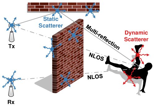
如图3所示，散射模型将室内环境中的所有物体视为散射体，将信号扩散到各个方向。接收器观察到的 CSI 与静态（家具、墙壁等）和动态（手臂、腿等）散射体贡献的部分相加。直观上，每个分散都被视为一个虚拟 Tx。这种建模可以应用于典型的室内场景，其中房间里挤满了家具，信号几乎可以向所有方向传播。在此基础上，我们可以忽略具体的信号传播路径，仅统计研究观测到的CSI与移动速度之间的关系。

我们将观察到的 CSI 分解为各个散射体贡献的部分：

(9)

H(f,t)=\sum_{o\in\Omega_{s}(t)}{H_{o}(f,t)}+\sum_{p\in\Omega_{d}(t)}{H_{p}(f,t)},

其中 $\Omega_{s}(t)$ 和 $\Omega_{d}(t)$ 是静态和动态散射体的集合， $H_{p}(f,t)$ 是由 $p^{th}$ 动态散射体贡献的观察到的CSI部分。对于每个散射体，扩散的分量经历匿名传播过程并最终在接收器处累加。尝试以 $p^{th}$ 散射体为原点，z轴与散射体运动方向一致的三维坐标，将 $H_{p}(f,t)$ 的表示进一步分解如下（张等人，2018）：

(10)

H_{p}(f,t)=\int_{0}^{2\pi}\int_{0}^{\pi}{h_{p}(\alpha,\beta,f,t)\exp(-jkv_{p}\cos(\alpha)t)\mathrm{d}\alpha\mathrm{d}\beta},

其中 $k=2\pi/\lambda$ 和 $\lambda$ 是信号波长， $v_{p}$ 是 $p^{th}$ 动态散射体的速度， $\alpha$ $\beta$ 为方位角和仰角， $\exp(-jkv_{i}\cos(\alpha)t)$ 表示信号在 $(\alpha,\beta)$ 方向上的相移。 $h_{p}(\alpha,\beta,f,t)$ 是 $p^{th}$ 散射体在 $(\alpha,\beta)$ 方向上贡献的观测到的 CSI 部分。继承于电磁波（Hill，2009）的物理特性， $h_{p}(\alpha,\beta,f,t)$ 可以被视为圆对称高斯随机变量。对于 $\forall p,q\in\Omega_{d}$ 和 $(\alpha_{1},\beta_{1})\neq(\alpha_{2},\beta_{2})$ , $h_{p}(\alpha_{1},\beta_{1},f,t)$ 独立于 $h_{q}(\alpha_{2},\beta_{2},f,t)$ 。

基于方程式。 9 和方程。 10，我们可以通过分析 $H(f,t)$ （Hill，2009）的自相关函数（ACF）得出统计特性：

(11)

\begin{split}\rho_{H}(f,\tau)&\triangleq\frac{\mathrm{Cov}[H(f,t),H(f,t+\tau)]}{\mathrm{Cov}[H(f,t),H(f,t)]}\\ &=\frac{\sum_{p\in\Omega_{d}}{\sigma_{p}^{2}(f)\mathrm{sinc}(kv\tau)}}{\sum_{p\in\Omega_{d}}{\sigma_{p}^{2}(f)}}\approx\mathrm{sinc}(kv\tau),\end{split}

其中 $\mathrm{Cov}[\cdot,\cdot]$ 是两个随机变量之间的协方差， $\sigma_{p}^{2}(f)$ 是 $h_{p}(\alpha,\beta,f,t)$ 、 $\mathrm{sinc}(kv\tau)=\frac{\sin(kv\tau)}{kv\tau}$ 和 $\tau$ 的方差> 是时间滞后。

对于一些人类活动，例如跌倒和行走，我们可以假设动态散射体主要位于躯干上，并且具有相似的速度 $v$ 。因此，等式。 11 近似为更简单的形式： $\rho_{H}(f,\tau)\approx\mathrm{sinc}(kv\tau)$ 。利用这个公式，我们定量地建立了 CSI 的人体速度和 ACF 之间的关系。实际上，速度 $v$ 是通过匹配 $\mathrm{sinc}(x)$ 函数的第一个峰值和ACF的第一个峰值来提取的：

(12)

v=\frac{x_{0}}{k\tau_{0}}=\frac{x_{0}\lambda}{2\pi\tau_{0}},

其中 $x_{0}$ 是代表 $\mathrm{sinc}(x)$ 函数第一个峰值位置的常数值， $\tau_{0}$ 是ACF第一个峰值对应的时间滞后。

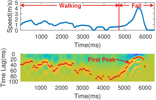
举一个简单的例子，我们让一名志愿者在一间布置齐全的房间里行走并摔倒，并使用从另一个房间的 Wi-Fi 链路收集的 CSI 来提取速度。如图4所示，即使存在非视距（NLoS）遮挡和多路径污染，步行速度和跌倒速度的估计也是一致的，证明了其对环境多样性的鲁棒性。

散射模型一般适用于各种面向速度的传感任务。散射模型一般适用于各种面向速度的传感任务，例如入侵检测和跌倒检测。作为一种统计模型，它在复杂场景下具有独特的优势。

然而，散射模型无法直接构建CSI和几何参数之间的对应关系，因此通常不适用于精确定位和跟踪任务。

3. CSI数据收集

CSI 数据收集是实现实用无线传感系统的第一步。本节介绍最著名的Wi-Fi传感数据集之一Widar3数据集，以便初学者可以以最小的努力快速开始无线传感。本节还介绍了三种最著名的 CSI 收集工具，研究人员可以使用它们尝试使用 COTS NIC 收集 CSI 数据。

3.1. Widar3 数据集

开放数据集对于提供模型训练的全面知识和模型比较的统一基准至关重要。在无线传感领域，开放数据集更加必要，因为射频信号对设备和部署环境更加敏感。然而，高质量、大规模数据集的缺乏成为阻碍无线传感技术进步的瓶颈。 2019年我们开始构建Widar3数据集时，现有的无线传感数据集规模较小，场景有限。 Widar3²²2http://tns.thss.tsinghua.edu.cn/widar3.0是用于人类活动识别的无线传感数据集。它以 RSSI 和 CSI 的形式从商用 Wi-Fi NIC 收集。它由来自 75 个领域的 258,000 个手势实例组成，持续时间为 8,620 分钟。 Widar3是迄今为止该领域最大、最全面的数据集，受到全世界研究人员的广泛关注。 Widar3 数据集在 IEEE DataPort（官方数据存储库）上公开提供，并不断发展以包含更多类型的活动。

3.2. PicoScenes 平台

PicoScenes (Jiang 等人, 2021) 是一款多功能且功能强大的中间件，用于基于 CSI 的 Wi-Fi 传感研究。它是极少数支持最新 802.11ac/ax 协议的工具之一。它支持许多流行的商用网卡，包括 Qualcomm Atheros AR9300 (QCA9300)、Intel Wireless Link 5300 (IWL5300)、Intel AX200 和 Intel AX210。 PicoScenes 支持最多 27 个 NIC 并发工作，以进行数据包注入和 CSI 测量。

PicoScenes 在架构上具有通用性和灵活性。它将所有低级功能封装成统一且独立于硬件的API，并将它们公开给上层插件层。因此，用户可以快速构建自己的测量插件原型。

PicoScenes 报告的数据可以在 MATLAB 中解析为结构体，其中包含不同数据包、子载波和天线的 CSI 数据。该结构还包括其他有用的信息，例如时间戳、RSSI 和信噪比 (SNR)。

首页³³3https://ps.zpj.io 以获取更多详细信息。

3.3. Intel 5300 NIC CSI 工具

此 CSI 工具（Halperin 等人，2011）基于 Intel WiFi Wireless Link 5300 802.11n MIMO 无线电构建，使用修改后的固件和开源 Linux 无线驱动程序。它包括收集、读取和解析 CSI 所需的所有软件和脚本。

IWL5300 提供 30 个子载波组的 802.11n CSI。每组包含 2 个给定 20 MHz 带宽的相邻子载波或 4 个给定 40 MHz 带宽的相邻子载波。每个 CSI 样本都是一个复数，实部和虚部均具有带符号的 8 位分辨率。一条CSI记录是一个 $A\times 30$ 矩阵，其中 $M$ 是发射和接收天线的对数。

首页⁴⁴4https://dhalperi.github.io/linux-80211n-csitool可以访问此工具以获取详细信息。

3.4. Atheros CSI 工具

Atheros CSI Tool (Xie 等人, 2018) 是一款开源 802.11n 测量和实验工具。它能够从 Atheros WiFi NIC 中提取详细的 PHY 无线通信信息，包括通道状态信息 (CSI)、接收到的数据包有效负载和其他信息（时间戳、每个天线的 RSSI、数据速率等）。）。 Atheros-CSI-Tool 构建于 ath9k 之上，ath9k 是一款支持 Atheros 802.11n PCI/PCI-E 芯片的开源 Linux 内核驱动程序。因此，该工具理论上支持所有类型的 Atheros 802.11n WiFi 芯片组。我们已在 Atheros AR9580、AR9590、AR9344 和 QCA9558 上进行了测试。此外，Atheros CSI Tool 是开源的，所有功能均以软件形式实现，无需对固件进行任何修改。因此，人们可以在 GPL 许可下使用自己的代码扩展 Atheros CSI Tool 的功能。

Atheros-CSI-Tool 适用于各种 Linux 发行版，例如 Ubuntu、OpenWRT、Linino 等。不同的 Linux 发行版适用于不同的硬件。 Ubuntu 适用于笔记本电脑或台式机等个人计算机。 OpenWRT 适用于 WiFi 路由器等嵌入式设备。 Linino 适用于 IoT 设备，例如 Arduino YUN。官网提供了Atheros CSI工具的Ubuntu版本和OpenWRT版本的源代码。

主页⁵⁵5https://wands.sg/research/WiFi/AtherosCSI以获取详细信息。

4. CSI特征提取

CSI 特性为无线传感奠定了基础。特别是，针对不同的传感任务，选择最合适的特征可以有效提高系统性能。此外，提取特征的质量决定了传感系统的有效性。

为了便于说明，下面提供了用于特征提取的代码实现，它是一个 main 函数，用于调用以下小节中的不同函数。

⬇

CSI Feature Extraction for Wi-Fi sensing.

- Input: csi data used for calibration, and csi data that need to be sanitized.

- Output: sanitized csi data.

To use this script, you need to:

1. Make sure the csi data have been saved as .mat files.

2. Check the .mat file to make sure they are in the correct form.

3. Set the parameters.

Note that in this algorithm, the csi data should be a 4-D tensor with the size of [T S A L]:

- T indicates the number of csi packets;

- S indicates the number of subcarriers;

- A indicates the number of antennas (i.e., the STS number in a MIMO system);

- L indicates the number of HT-LTFs in a single PPDU;

Say if we collect a 10 seconds csi data steam at 1 kHz sample rate (T = 10 * 1000), from a 3-antenna AP (A = 3), with 802.11n standard (S = 57 subcarrier), without any extra spatial sounding (L = 1), the data size should be [10000 57 3 1].

clear all;

addpath(genpath(pwd));

%% 0. Set parameters.

% Path of the raw CSI data.

src_file_name = ’./data/csi_src_test.mat’;

% Speed of light.

global c;

c = physconst(’LightSpeed’);

% Bandwidth.

global bw;

bw = 20e6;

% Subcarrier frequency.

global subcarrier_freq;

subcarrier_freq = linspace(5.8153e9, 5.8347e9, 57);

% Subcarrier wavelength.

global subcarrier_lambda;

subcarrier_lambda = c ./ subcarrier_freq;

% Antenna arrangement.

antenna_loc = [0, 0, 0; 0.0514665, 0, 0; 0, 0.0514665, 0]’;

% Set the linear range of the CSI phase, which varies with NIC types.

linear_interval = (20:38)’;

%% 1. Read the csi data for calibration and sanitization.

% Load the raw CSI data.

csi_src = load(src_file_name).csi; % Raw CSI.

%% 2. Perform various wireless sensing tasks.

% Test example 1: angle/direction estimation with imperfect CSI.

[packet_num, subcarrier_num, antenna_num, ~] = size(csi_src);

aoa_mat = naive_aoa(csi_src, antenna_loc, zeros(3, 1));

aoa_gt = [0; 0; 1];

error = mean(acos(aoa_gt’ * aoa_mat));

disp("Angle estimation error: " + num2str(error));

% Test example 2: distance estimation with CSI.

tof_mat = naive_tof(csi_src);

est_dist = mean(tof_mat * c, ’all’);

disp("The ground truth distance is: 10 m");

disp("The estimated distance is: " + num2str(est_dist) + " m");

4.1. 飞行时间

ToF 是信号沿特定路径从发射器传播到接收器的持续时间。给定频率 $f$ ，ToF $\tau$ 引入的相移为：

(13)

\phi_{\mathrm{ToF}}=-2\pi f\tau

CSI作为多径信号的叠加，可以基于射线追踪模型来表示：

(14)

H(f)=\sum_{n=1}^{N}\alpha_{n}e^{-j2\pi f\tau_{n}}

其中 $N$ 是多径总数， $\alpha_{n}$ 和 $\tau_{n}$ 是 $n^{th}$ 理论上，所有路径的ToF都可以在CIR中识别，CIR可以通过对所有子载波的CSI样本进行傅里叶逆变换来计算。然而，由于发射器和接收器缺乏同步，CIR 中存在非零时间偏移，并且绝对 ToF 通常不够准确。有限的带宽也限制了时间分辨率，导致米级ToF模糊度。信号传播路径、ToF和CIR之间的关系如图5所示。

下面的函数naive_tof旨在基于傅里叶逆变换提取最强路径（通常是最短路径）的ToF。

⬇

function [tof_mat] = naive_tof(csi_data)

% naive_tof

% Input:

% - csi_data is the CSI used for ranging; [T S A E]

% - ifft_point and bw are the IFFT and bandwidth parameters;

% Output:

% - tof_mat is the rough time-of-flight estimation result; [T A]

global c, bw;

[pakcet_num, subcarrier_num, antenna_num, extra_num] = size(csi_data);

ifft_point = power(2, ceil(log2(subcarrier_num)));

% Get CIR from each packet and each antenna by ifft(CFR);

cir_sequence = zeros(packet_num, antenna_num, extra_num, ifft_point);

for p = 1:packet_num

for a = 1:antenna_num

for e = 1:extra_num

cir_sequence(p, a, e, :) = ifft(csi_data(p, :, a, e), ifft_point);

end

cir_sequence = squeeze(mean(cir_sequence, 4)); % [T ifft_point A]

half_point = ifft_point / 2;

half_sequence = cir_sequence(:, 1:half_point, :); % [T half_point A]

peak_indices = zeros(packet_num, antenna_num); % [T A]

for p = 1:pakcet_num

for a = 1:antenna_num

[~, peak_indices(p, a)] = max(half_sequence, [], 2);

end

% Calculate ToF;

tof_mat = peak_indices .* subcarrier_num ./ (ifft_point .* bw); % [T A]

end

4.2. 到达角和出发角

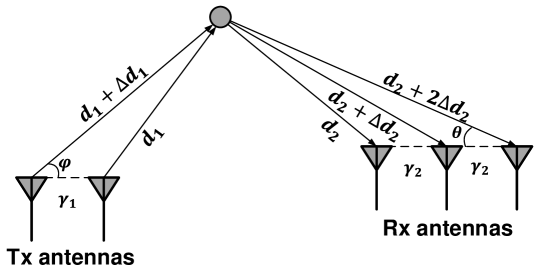
当网卡配备多个天线时，可以在设备上创建本地坐标。如图6所示，对于发射机来说，出发角（AoD） $\varphi$ 表示本地坐标中发射信号的发射方向。对于接收器而言，到达角 (AoA) $\theta$ 表示捕获接收信号时沿本地坐标的方向。由于天线在空间上分离，因此在天线之间引入非零相移。相移取决于 AoA/AoD。具体来说，假设两天线之间的相对位置为 ${\boldsymbol{\Delta{l}}}=(\Delta_{x},\Delta_{y})$ ，迎角单位方向向量为 ${\boldsymbol{e}}=(cos\theta,\sin\theta)$ ，则两天线之间的相移为：

(15)

\phi_{\mathrm{AoA}}=\frac{2\pi}{\lambda}{\boldsymbol{\Delta{l}}}\cdot{\boldsymbol{e}}

那么 CSI 可以建模为：

(16)

H(k)=\sum_{n=1}^{N}\alpha_{n}e^{-j\frac{2\pi}{\lambda}{\boldsymbol{\Delta{l}}}\cdot{\boldsymbol{e}}}

其中 $k$ 表示接收器处的 $k^{th}$ 天线。相同的模型适用于发射机侧的 AoD 以及具有方位角和仰角的 3D 空间。

在实践中，Capon （Capon，1969）和MUSIC （Schmidt，1986）等算法可用于根据信道的CSI估计多条路径的AoA/AoD。天线阵列。

MUSIC 分析多个天线上的入射信号，找出每个信号的迎角。具体来说，假设 $D$ 信号 $F_{1},\cdots,F_{D}$ 从 $\theta_{1},\cdots,\theta_{D}$ 方向到达 $M>D$ 天线。 $k^{th}$ 天线元件处的接收信号表示为 $X_{k}$ ，是 $D$ 入射波前和噪声 $W_{k}$ 的线性组合：

\left[\begin{array}[]{c}X_{1}\\ X_{2}\\ \vdots\\ X_{M}\end{array}\right]=\left[\begin{array}[]{llll}{\boldsymbol{a}}(\theta_{1})&{\boldsymbol{a}}(\theta_{2})&\ldots&{\boldsymbol{a}}(\theta_{D})\end{array}\right]\left[\begin{array}[]{c}F_{1}\\ F_{2}\\ \vdots\\ F_{D}\end{array}\right]+\left[\begin{array}[]{c}W_{1}\\ W_{2}\\ \vdots\\ W_{M}\end{array}\right]

或者

(17)

{\boldsymbol{X}}={\boldsymbol{AF}}+{\boldsymbol{W}}

其中 $\mathbf{a}(\theta_{k})$ 是阵列导向矢量，表征 $k^{th}$ 天线处每个接收组件的附加相位（相对于第一天线）。 ${\boldsymbol{A}}$ 是转向向量矩阵。如图6所示，对于阵元同步良好的线性天线阵列，

(18)

{\boldsymbol{a}}(\theta)=\left[\begin{array}[]{c}1\\ e^{-j\frac{2\pi}{\lambda}{\boldsymbol{\Delta{l(1)}}}\cdot{\boldsymbol{e}}}\\ e^{-j\frac{2\pi}{\lambda}{\boldsymbol{\Delta{l(2)}}}\cdot{\boldsymbol{e}}}\\ \vdots\\ e^{-j\frac{2\pi}{\lambda}{\boldsymbol{\Delta{l(M-1)}}}\cdot{\boldsymbol{e}}}\end{array}\right]

假设 $W_{k}\sim N(0,\sigma^{2})$ 、 $F_{k}$ 是均值为零的广义平稳过程，则接收信号向量 ${\boldsymbol{X}}$ 的 $M\times M$ 协方差矩阵> 是：

(19)	$\displaystyle{\boldsymbol{S}}$	$\displaystyle=\overline{{\boldsymbol{XX}}^{\mathrm{H}}}$
		$\displaystyle={\boldsymbol{A}}\overline{{\boldsymbol{FF}}^{\mathrm{H}}}{\boldsymbol{A}}^{\mathrm{H}}+\overline{{\boldsymbol{WW}}^{\mathrm{H}}}$
		$\displaystyle={\boldsymbol{APA}}^{\mathrm{H}}+\sigma^{2}{\boldsymbol{I}}$

其中 ${\boldsymbol{P}}$ 是传输向量 ${\boldsymbol{F}}$ 的协方差矩阵。符号 $(\cdot)^{\mathrm{H}}$ 表示共轭转置， $\overline{(\cdot)}$ 表示期望。

协方差矩阵 ${\boldsymbol{S}}$ 具有与 $M$ 特征向量 ${\boldsymbol{e}}_{1},{\boldsymbol{e}}_{2},\cdots,{\boldsymbol{e}}_{M}$ 关联的 $M$ 特征值 $\lambda_{1},\cdots,\lambda_{M}$ 。按非降序排序，最小的 $M-D$ 特征值对应于噪声，而其余的 $D$ 对应于 $D$ 事件信号。换句话说， $M$ 维空间可以分为两个正交子空间，由特征向量 ${\boldsymbol{e}}_{1},\cdots,{\boldsymbol{e}}_{M-D}$ 扩展的噪声子空间 ${\boldsymbol{E}}_{N}$ 和信号子空间 ${\boldsymbol{E}}_{S}$ 由特征向量 ${\boldsymbol{e}}_{M-D+1},\cdots,{\boldsymbol{e}}_{M}$ 扩展（或等效的 $D$ 数组导向向量 ${\boldsymbol{a}}(\theta_{1}),\cdots,{\boldsymbol{a}}(\theta_{D})$ )。

为了求解阵列转向矢量（即 AoA），MUSIC 绘制了沿 $\theta$ 继续到噪声子空间的点的平方距离 $Q(\theta)$ 的倒数，作为 $\theta$

(20)

Q(\theta)=\frac{1}{{\boldsymbol{a}}^{\mathrm{H}}(\theta){\boldsymbol{E}}_{N}{\boldsymbol{E}}_{N}^{\mathrm{H}}{\boldsymbol{a}}(\theta)}

这会在入射信号的方位处产生 $Q(\theta)$ 峰值。与应用MUSIC算法进行AoD频谱估计类似。

下面的函数naive_aoa旨在根据相位差估计3D AoA，这与等式1类似。 15. 请注意，以下算法仅考虑一条路径，因此不能应用于多路径信号。

⬇

function [aoa_mat] = naive_aoa(csi_data, antenna_loc, est_rco)

% naive_aoa

% Input:

% - csi_data is the CSI used for angle estimation; [T S A E]

% - antenna_loc is the antenna location arrangement with the first antenna as a reference; [3 A]

% - est_rco is the estimated radio chain offset; [A 1]

% Output:

% - aoa_mat is the angle estimation result; [3 T]

global subcarrier_lambda;

[packet_num, subcarrier_num, antenna_num, extra_num] = size(csi_data);

csi_phase = unwrap(angle(csi_data), [], 2); % [T S A E]

% Get the antenna vector and its length.

ant_diff = antenna_loc(:, 2:end) - antenna_loc(:, 1); % [3 A-1]

ant_diff_length = vecnorm(ant_diff); % [1 A-1]

ant_diff_normalize = ant_diff ./ ant_diff_length; % [3 A-1]

% Calculate the phase difference.

phase_diff = csi_phase(:, :, 2:end, :) - csi_phase(:, :, 1, :) - permute(est_rco(2:end, :), [4 3 1 2]); % [T S A-1 E]

phase_diff = unwrap(phase_diff, [], 2);

phase_diff = mod(phase_diff + pi, 2 * pi) - pi;

% Broadcasting is performed, get the value of cos(theta) for each packet and each antenna pair.

cos_mat = subcarrier_lambda .* phase_diff ./ (2 .* pi .* permute(ant_diff_length, [3 1 2])); % [T S A-1 E]

cos_mat_mean = squeeze(mean(cos_mat, [2 4])); % [T A-1]

% Symbolic nonlinear optimization are performed.

syms x y

% aoa_sol = [x;y;(1-sqrt(x^2 + y^2))];

aoa_init = [sqrt(1/3);sqrt(1/3);sqrt(1/3)];

aoa_mat_sol = zeros(3, packet_num);

options = optimoptions(’lsqnonlin’, ’Algorithm’, ’levenberg-marquardt’, ’Display’, ’none’);

parfor p = 1:packet_num

cur_nonlinear_func = @(aoa_sol)ant_diff_normalize’ * aoa_sol - cos_mat_mean(p, :)’;

cur_aoa_sol = lsqnonlin(cur_nonlinear_func, aoa_init, [], [], options);

aoa_mat_sol(:, p) = cur_aoa_sol;

end

aoa_mat = aoa_mat_sol ./ vecnorm(aoa_mat_sol); % [3 T]

end

4.3. 相移频谱

不同数据包之间的非零相移 $\Delta\phi$ 是由信号传播路径中的发射器、接收器或物体的相对运动引起的。它等于信号路径长度的变化率。当依次接收到多个数据包时， $i^{th}$ 接收到的数据包对应的CSI为：

(21)

H(i)=\sum_{n=1}^{N}\alpha_{n}(i)e^{j\phi_{n}(i)},

其中 $\phi_{n}$ 是 $n^{th}$ 路径 (Chi 等人, 2022) 的阶段。分别提取数据包 $i$ 和 $i+1$ 中 $n^{th}$ 路径的相位，并计算相移为：

(22)

\Delta\phi_{n}(i)=\phi_{n}(i+1)-\phi_{n}(i).

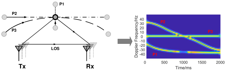
直观上，相位差表示两个连续数据包 $\Delta d_{n}(i)=\frac{\Delta\phi_{n}(i)}{2\pi}\lambda$ 之间 $n^{th}$ 路径的距离变化。

更进一步，在滑动窗口内应用短时傅立叶变换（STFT），我们可以得到如图7所示的频谱。频率轴揭示了连续CSI数据的变化率，并且隐含地包含路径长度变化率。图7展示了三个不同移动路径的相移频谱（或多普勒频谱）。

以下函数naive_stft计算一系列CSI数据的短时傅立叶变换。生成的频谱可有效用于许多无线传感任务，例如手势识别和跌倒检测。

⬇

function stft_mat = naive_spectrum(csi_data, sample_rate, visable)

% naive_spectrum

% Input:

% - csi_data is the CSI used for STFT spectrum generation; [T S A L]

% - sample_rate determines the resolution of the time-domain and

% frequency-domain;

% Output:

% - stft_mat is the generated STFT spectrum; [sample_rate/2 T]

% Conjugate multiplication.

csi_data = mean(csi_data .* conj(csi_data), [2 3 4]);

% Calculate the STFT and visualization.

stft_mat = stft(csi_data, sample_rate);

% Visualization (optional).

if visable

stft(csi_data, sample_rate);

end

4.4. 身体坐标速度曲线

上述频谱的局限性在于，当用户相对于Wi-Fi链路移动到不同的位置或方向时，即使是相同的活动对应的频谱也会不同。为了解决这个问题，Widar3.0（Zheng等人，2019）提出了一种与域无关的信号特征BVP（身体坐标速度剖面）来表征人类活动。

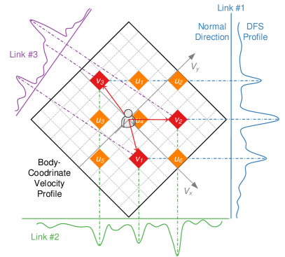
BVP的基本思想如图8所示。 BVP ${\boldsymbol{V}}$ 被量化为离散矩阵，其维度为沿身体坐标的每个轴分解的速度分量。为了方便起见，我们建立局部身体坐标，其原点是人的位置，正 x 轴与人的方向对齐。应手动提供人员的位置和方向。目前，假设人的全球位置和方向可用。然后，可以将无线收发器的已知全球位置转换为局部身体坐标。因此，为了更清楚起见，以下推导中使用的所有位置和方向均采用局部身体坐标。假设 $i^{th}$ 链路的发射器和接收器的位置分别为 $\vec{l}_{t}^{(i)}=(x_{t}^{(i)},y_{t}^{(i)})$ 、 $\vec{l}_{r}^{(i)}=(x_{r}^{(i)},y_{r}^{(i)})$ ，则周围的任何速度分量 $\vec{v}=(v_{x},v_{y})$ 人体（即原点）会将其信号功率贡献给 $i^{th}$ 链路的多普勒频谱中的某个频率分量，记为 $f^{(i)}(\vec{v})$ （Qian 等人，2017）：

(23)

f^{(i)}(\vec{v})=a_{x}^{(i)}v_{x}+a_{y}^{(i)}v_{y}.

$a_{x}^{(i)}$ 和 $a_{y}^{(i)}$ 是由发射器和接收器的位置确定的系数：

(24)		$\displaystyle a_{x}^{(i)}=\frac{1}{\lambda}(\frac{x_{t}^{(i)}}{\\|\vec{l}_{t}^{(i)}\\|_{2}}+\frac{x_{r}^{(i)}}{\\|\vec{l}_{r}^{(i)}\\|_{2}}),$
(24)		$\displaystyle a_{y}^{(i)}=\frac{1}{\lambda}(\frac{y_{t}^{(i)}}{\\|\vec{l}_{t}^{(i)}\\|_{2}}+\frac{y_{r}^{(i)}}{\\|\vec{l}_{r}^{(i)}\\|_{2}}),$

其中 $\lambda$ 是Wi-Fi信号的波长。由于在计算多普勒频谱之前滤除具有零多普勒频谱的静态分量（例如，视线信号和静态物体的主要反射），因此仅保留人反射的信号。此外，当人靠近Wi-Fi链路时，只有一次性反射的信号才会具有显着的幅度（Qian等人，2018）。因此，等式。 23 对于手势识别场景有效。从几何角度来看，方程。 23表示二维速度矢量 $\vec{v}$ 投影在方向矢量为 ${\boldsymbol{d}}^{(i)}=(-a_{y}^{(i)},a_{x}^{(i)})$ 的线上。假设人位于椭圆曲线上，其焦点是 $i^{th}$ 链路的发射器和接收器，则 $d^{(i)}$ 确实是人所在位置的椭圆的平均方向。图8显示了人生成三个速度分量 $\vec{v}_{j},j=1,2,3$ 的示例，以及速度分量在三个链路的多普勒频谱上的投影。

由于系数 $a_{x}^{(i)}$ 和 $a_{y}^{(i)}$ 仅取决于 $i^{th}$ 链接的位置，因此BVP在 $i^{th}$ 链接上的投影关系是固定的。具体来说，可以定义一个赋值矩阵 ${\boldsymbol{A}}^{(i)}_{F\times N^{2}}$ ：

(25)

A^{(i)}_{j,k}=\left\{\begin{array}[]{ll}1&f_{j}=f^{(i)}(\vec{v}_{k})\\ 0&{\rm else}\end{array}\right.,

其中 $f_{j}$ 是多普勒频谱中的 $j^{th}$ 频率采样点， $\vec{v}_{k}$ 是矢量化向量的 $k^{th}$ 元素对应的速度分量。 BVP ${\boldsymbol{V}}$ 。因此， $i^{th}$ 链路的多普勒频谱轮廓与BVP之间的关系可以建模为：

(26)

{\boldsymbol{D}}^{(i)}=c^{(i)}{\boldsymbol{A}}^{(i)}{\boldsymbol{V}}

其中 $c^{(i)}$ 是由于反射信号的传播损失而产生的缩放因子。

由于BVP的稀疏性，可以采用压缩感知（Donoho，2006）技术将BVP的估计表示为 $l_{0}$ 优化问题：

(27)

{\rm min}_{V}\sum_{i=1}^{M}|{\rm EMD}({\boldsymbol{A}}^{(i)}{\boldsymbol{V}},{\boldsymbol{D}}^{i})|+\eta\|V\|_{0},

其中 $M$ 是 Wi-Fi 链接的数量。速度分量数量的稀疏性由术语 $\eta\|V\|_{0}$ 强制，其中 $\eta$ 表示稀疏系数， $\|\cdot\|_{0}$ 是非零速度的数量成分。

${\rm EMD}(\cdot,\cdot)$ 是两个分布之间的推土机距离（Rubner 和 Tomasi，2001）。选择 EMD 而不是欧氏距离主要有两个原因。首先，BVP 的量化引入了近似误差，即速度分量到多普勒频谱箱的投影可能与真实的投影相邻。这种量化误差可以通过 EMD 来缓解，EMD 考虑了 bin 之间的距离。其次，BVP 和多普勒频谱之间存在未知的缩放因子，使得欧几里得距离不适用。

5. CSI 清理

前面几节中描述的无线传感模型和特征与电磁传播理论和几何结构一致。然而，他们没有考虑由于收发器硬件实现不完善而导致的各种类型的噪声（Xie等人，2018；Xie等人，2019）。本节重点介绍各种 CSI 错误源以及相应的错误消除算法。

为了便于说明，提供了清理的代码实现，它是一个 main 函数，用于调用不同的错误取消函数并测试其性能。

⬇

CSI Sanitization Algorithm for Wi-Fi sensing.

- Input: csi data used for calibration, and csi data that need to be sanitized.

- Output: sanitized csi data.

To use this script, you need to:

1. Make sure the csi data have been saved as .mat files.

2. Check the .mat file to make sure they are in the correct form.

3. Set the parameters.

Note that in this algorithm, the csi data should be a 4-D tensor with the size of [T S A L]:

- T indicates the number of csi packets;

- S indicates the number of subcarriers;

- A indicates the number of antennas (i.e., the STS number in a MIMO system);

- L indicates the number of HT-LTFs in a single PPDU;

Say if we collect a 10 seconds csi data steam at 1 kHz sample rate (T = 10 * 1000), from a 3-antenna AP (A = 3), with 802.11n standard (S = 57 subcarrier), without only one spatial stream (L = 1), the data size should be [10000 57 3 1].

clear all;

addpath(genpath(pwd));

%% 0. Set parameters.

% Path of the calibration data;

calib_file_name = ’./data/csi_calib_test.mat’;

% Path for storing the generated calibration templated.

calib_template_name = ’./data/calib_template_test.mat’;

% Path of the raw CSI data.

src_file_name = ’./data/csi_src_test.mat’;

% Path for storing the sanitized CSI data.

dst_file_name = ’./data/csi_dst_test.mat’;

% Speed of light.

global c;

c = physconst(’LightSpeed’);

% Bandwidth.

global bw;

bw = 20e6;

% Subcarrier frequency.

global subcarrier_freq;

subcarrier_freq = linspace(5.8153e9, 5.8347e9, 57);

% Subcarrier wavelength.

global subcarrier_lambda;

subcarrier_lambda = c ./ subcarrier_freq;

% Antenna arrangement.

antenna_loc = [0, 0, 0; 0.0514665, 0, 0; 0, 0.0514665, 0]’;

% Set the linear range of the CSI phase, which varies with NIC types.

linear_interval = (20:38)’;

%% 1. Read the csi data for calibration and sanitization.

% Load the calibration data.

csi_calib = load(calib_file_name).csi; % CSI for calibration.

% Load the raw CSI data.

csi_src = load(src_file_name).csi; % Raw CSI.

%% 2. Choose different functions according to your task.

% Use cases:

% Make calibration template.

csi_calib_template = set_template(csi_calib, linear_interval, calib_template_name);

% Directly load the generated template.

csi_calib_template = load(calib_template_name).csi;

% Remove the nonlinear error.

csi_remove_nonlinear = nonlinear_calib(csi_src, csi_calib_template);

% Remove the STO (a.k.a SFO and PBD) by conjugate mulitplication.

csi_remove_sto = sto_calib_mul(csi_src);

% Remove the STO (a.k.a SFO and PBD) by conjugate division.

csi_remove_sto = sto_calib_div(csi_src);

% Estimate the CFO by frequency tracking.

est_cfo = cfo_calib(csi_src);

% Estimate the RCO.

est_rco = rco_calib(csi_calib);

%% 3. Save the sanitized data as needed.

csi = csi_remove_sto;

save(dst_file_name, ’csi’);

%% 4. Perform various wireless sensing tasks.

% Test example 1: angle/direction estimation with imperfect CSI.

[packet_num, subcarrier_num, antenna_num, ~] = size(csi_src);

est_rco = rco_calib(csi_calib);

zero_rco = zeros(antenna_num, 1);

aoa_mat_error = naive_aoa(csi_src, antenna_loc, zero_rco);

aoa_mat = naive_aoa(csi_src, antenna_loc, est_rco);

aoa_gt = [0; 0; 1];

error_1 = mean(acos(aoa_gt’ * aoa_mat_error));

error_2 = mean(acos(aoa_gt’ * aoa_mat));

disp("Angle estimation error (in deg) without RCO removal: " + num2str(error_1));

disp("Angle estimation error (in deg) with RCO removal: " + num2str(error_2));

% Test example 2: intrusion detection with CSI.

csi_sto_calib = sto_calib_div(csi_src);

intrusion_flag_raw = naive_intrusion(csi_src, 3);

intrusion_flag_sanitized = naive_intrusion(csi_sto_calib, 3);

disp("Intrusion detection result without SFO/PDD removal: " + num2str(intrusion_flag_raw));

disp("Intrusion detection result with SFO/PDD removal: " + num2str(intrusion_flag_sanitized));

5.1. 非线性幅度和相位

非线性幅度和相位误差是由硬件内部不完善的模拟域滤波器实现引起的。具体来说，它使得提取的CSI幅度和相位被非线性函数等效地处理。令 $f(\cdot)$ 和 $g(\cdot)$ 分别为CSI幅度和相位的非线性模式，则错误CSI可写为：

(28)

\tilde{H}(i,j,k)=\sum_{n=1}^{N}{f(\alpha_{n})e^{-jg(\phi_{n}(i,j,k))}}+N(i,j,k).

具体地，在OFDM调制过程中，每个子载波应该具有相同的增益。换句话说，当使用同轴电缆连接收发器端口时，CSI的幅频特性应该是一条水平直线。但实际测量表明，即使没有多径无线信道，仍然存在类似的“频率选择性衰落”特性，即各个频段的增益不同，呈现M形幅频特性曲线。同样，当使用同轴电缆连接收发端口时，NIC获得的CSI相频特性也不是一条带有斜率的理想直线，而是一条具有一定非线性的S形曲线。

经过广泛的研究和实验，我们观察到两个事实。

•

首先，对于特定类型的NIC，CSI的非线性幅度/相位误差是固定的。这意味着如果我们使用连接到收发器端口的已知长度的同轴电缆就可以完成校正任务。在执行感知任务之前，测量一组代表性的CSI幅度和相位，记录非线性特征，并在后续步骤中消除非线性。
•

其次，我们观察到子载波的中间部分没有非线性误差，并且两侧的非线性特性也是固定的。

因此，代码下面的函数执行以下步骤来解决 CSI 非线性问题：

(1)

读入使用同轴电缆测量的一组 CSI 数据。
(2)

获取其幅度和相位。
(3)

对其幅度进行归一化并将其记录为幅度模板。
(4)

展开相位，然后对其子载波的中间部分执行线性拟合。减去线性拟合结果即可得到非线性相位误差模板。

最后将非线性幅度和非线性相位分量以 $\alpha e^{j\phi}$ 的形式保存，表示特定类型网卡的非线性误差模板。

⬇

function [csi_calib_template] = set_template(csi_calib, linear_interval, calib_template_name)

% set_template

% Input:

% - csi_calib is the reference csi at given distance and angle; [T S A L]

% - linear_interval is the linear range of the csi phase, which varies across different types of NICs;

% - calib_template_name is the saved path of the generated template;

% Output:

% - csi_calib_template is the generated template for csi calibration; [1 S A L]

[packet_num, subcarrier_num, antenna_num, extra_num] = size(csi_calib);

csi_amp = abs(csi_calib); % [T S A L]

csi_phase = unwrap(angle(csi_calib), [], 2); % [T S A L]

csi_amp_template = mean(csi_amp ./ mean(csi_amp, 2), 1); % [1 S A L]

nonlinear_phase_error = zeros(size(csi_calib)); % [T S A L]

for p = 1:packet_num

for a = 1:antenna_num

for e = 1:extra_num

linear_model = fit(linear_interval, squeeze(csi_phase(p, linear_interval, a, e))’, ’poly1’);

nonlinear_phase_error(p, :, a, e) = csi_phase(p, :, a, e) - linear_model(1:subcarrier_num)’;

end

csi_phase_template = mean(nonlinear_phase_error, 1); % [1 S A L]

csi_phase_template(1, linear_interval, :, :) = 0;

csi_calib_template = csi_amp_template .* exp(1i * csi_phase_template); % [1 S A L]

csi = csi_calib_template;

save(calib_template_name, ’csi’); % [1 S A L]

end

获得非线性误差模板后，净化过程开始。对于实时收集的原始CSI数据csi_data，我们将其除以误差模板csi_calib。这个操作相当于“原始幅度除以归一化非线性幅度”和“非线性相位减去原始相位”，这样返回的CSI数据csi_proc就已经净化了幅度和相位。

⬇

function [csi_remove_nonlinear] = nonlinear_calib(csi_calib, csi_calib_template)

% nonlinear_calib

% Input:

% - csi_src is the raw csi which needs to be calibrated; [T S A L]

% - csi_calib_template is the reference csi for calibration; [1 S A L]

% Output:

% - csi_remove_nonlinear is the csi data in which the nonlinear error has been eliminated; [T S A L]

csi_amp = abs(csi_calib); % [T S A L]

csi_phase = unwrap(angle(csi_calib), [], 2); % [T S A L]

csi_unwrap = csi_amp .* exp(1i * csi_phase); % [T S A L]

% Broadcasting is performed.

csi_remove_nonlinear = csi_unwrap ./ csi_calib_template;

end

5.2. 自动增益控制不确定度

自动增益控制 (AGC) 在每个接收到的 CSI 数据包中引入随机增益 $\beta$ 。

(29)

\tilde{H}(i,j,k)=\sum_{n=1}^{N}{\beta_{i}\alpha_{n}e^{-j\phi_{n}(i,j,k)}}+N(i,j,k).

消除AGC误差的方法有两种： 1）禁用无线驱动的AGC功能； 2) 根据报告的AGC 补偿测量的CSI 的幅度。

⬇

function [csi_remove_agc] = agc_calib(csi_src, csi_agc)

% rco_calib

% Input:

% - csi_src is the raw csi which needs to be calibrated; [T S A L]

% - csi_agc is the AGC amplitude reported by the NIC; [T, 1]

% Output:

% - csi_remove_agc is the csi data in which the AGC uncertainty has been eliminated; [T S A L]

% Broadcasting is performed.

csi_remove_agc = csi_src ./ csi_agc;

end

5.3. 无线电链偏移

无线电链偏移 (RCO) 是不同 Tx/Rx 链（收发器天线对）之间引入的随机相位变化 $\epsilon_{\phi}$ 。每次 NIC 通电时，RCO 都会重置。

(30)

\tilde{\phi}_{n}(i,j,k)=2\pi(f_{c}+\Delta f_{j}+f_{D})\tau_{n}(i,j,k)+\epsilon_{\phi},

RCO 会引起相频特性曲线的偏差。它会降低 AoA 或 ToF 等特征的准确性。幸运的是，我们发现这种类型的相位偏差在发送的每个连续数据包之间是一致的，因此不会影响时间跟踪或感测的性能，并且可以通过以下步骤消除这种类型的错误：

(1)

NIC 上电后，使用已知长度的同轴电缆连接收发器端口并记录相位信息calib_phase。
(2)

在后续测量期间，从测量的相位csi_phase中减去该相位信息。

⬇

function [est_rco] = rco_calib(csi_calib)

% rco_calib

% Input:

% - csi_calib is the reference csi at given distance and angle; [T S A L]

% Output:

% - est_rco is the estimated RCO; [A 1]

antenna_num = size(csi_calib, 3);

csi_phase = unwrap(angle(csi_calib), [], 1); % [T S A L]

avg_phase = zeros(antenna_num, 1);

for a = 1:antenna_num

avg_phase(a, 1) = mean(csi_phase(:, :, a, 1), ’all’);

end

est_rco = avg_phase - avg_phase(1, 1);

end

5.4. 中心频率偏移

中心频率偏移（CFO）是由收发器两侧频率不同步引起的，导致每个接收到的CSI出现随机频移 $\epsilon_{f}$ 。

(31)

\tilde{\phi}_{n}(i,j,k)=2\pi(f_{c}+\Delta f_{j}+f_{D}+\epsilon_{f})\tau_{n}(i,j,k)=\phi_{n}(i,j,k)+\epsilon_{f}\tau_{n}(i,j,k).

CFO 会引起相频特性曲线的额外偏差（即整体上移和下移）。

为了消除CFO，我们需要在同一个PPDU（Wi-Fi数据帧）中插入多个HT-LTF，从而获得多个CSI测量。由于根据802.11协议，多个HT-LTF之间的时间间隔被严格控制在 $4\mu s$ ，因此两个HT-LTF之间的相位差是由CFO在 $\Delta t=4\mu s$ 内引起的。这样就可以恢复出CFO的近似值。

⬇

function [est_cfo] = cfo_calib(csi_src)

% cfo_calib

% Input:

% - csi_src is the csi data with two HT-LTFs; [T S A L]

% Output:

% - est_cfo is the estimated frequency offset;

delta_time = 4e-6;

phase_1 = angle(csi_src(:, :, :, 1));

phase_2 = angle(csi_src(:, :, :, 2));

phase_diff = mean(phase_2 - phase_1, 3); % [T S A 1]

est_cfo = mean(phase_diff ./ delta_time, 2);

end

5.5. 采样频率偏移和数据包检测延迟

采样频率偏移（SFO）在频域中表现为一个误差，通常被认为是由于频率异步导致的等效时移。数据包检测延迟（PDD）是时间延迟。因此，尽管它们的原因不同，但它们经常被一起讨论为“时间偏移”。

(32)

\tilde{\phi}_{n}(i,j,k)=2\pi(f_{c}+\Delta f_{j}+f_{D})(\tau_{n}(i,j,k)+\epsilon_{t})=\phi_{n}(i,j,k)+2\pi(f_{c}+\Delta f_{j}+f_{D})\epsilon_{t}.

这种类型的误差非常严重，因为时间延迟可能与真实的 ToF 混淆，从而影响测距精度。具体地，该偏差在相频特性曲线中将被表征为斜率的变化，因为该时间偏差对于不同的子带 $\Delta f_{j}$ 造成不同的相位变化。

目前，还没有“完美的算法”来解决此类错误。共轭乘法和除法是消除 SFO 和 PDD 的唯一两种方法。下面列出了它们的代码。通过应用共轭乘法或除法， $\epsilon_{t}$ 被消除，但代价是失去绝对 ToF 测量。

⬇

function [csi_remove_sto] = sto_calib_mul(csi_src)

% sto_calib_mul

% Input:

% - csi_src is the csi data with sto; [T S A L]

% Output:

% - csi_remove_sto is the csi data without sto; [T S A L]

antenna_num = size(csi_src, 3);

csi_remove_sto = zeros(size(csi_src));

for a = 1:antenna_num

a_nxt = mod(a, antenna_num) + 1;

csi_remove_sto(:, :, a, :) = csi_src(:, :, a, :) .* conj(csi_src(:, :, a_nxt, :));

end

⬇

function [csi_remove_sto] = sto_calib_div(csi_src)

% sto_calib_div

% Input:

% - csi_src is the csi data with sto; [T S A L]

% Output:

% - csi_remove_sto is the csi data without sto; [T S A L]

antenna_num = size(csi_src, 3);

csi_remove_sto = zeros(size(csi_src));

for a = 1:antenna_num

a_nxt = mod(a, antenna_num) + 1;

csi_remove_sto(:, :, a, :) = csi_src(:, :, a, :) ./ csi_src(:, :, a_nxt, :);

end

综上所述，Wi-Fi CSI 测量中存在多种形式的误差，包括固定偏差和随机误差。它们每个对定位、跟踪和传感任务都有不同的影响。错误的CSI形式最终可以写成：

(33)

\tilde{H}(i,j,k)=\sum_{n=1}^{N}{\beta_{i}f(\alpha_{n})e^{-jg(\phi_{n}(i,j,k))}}+N(i,j,k),\\ \tilde{\phi}_{n}(i,j,k)=2\pi(f_{c}+\Delta f_{j}+f_{D}+\epsilon_{f})(\tau_{n}(i,j,k)+\epsilon_{t})+\epsilon_{\phi}.

6. 深度学习无线传感

本节介绍一系列学习算法，特别是当前流行的深度神经网络模型，如CNN和RNN，及其在无线传感中的应用。本节还提出了一种复值神经网络来有效地完成基于无线特征的学习和推理。

6.1. 卷积神经网络

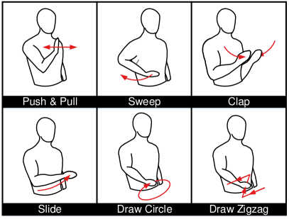
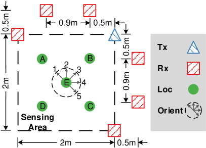
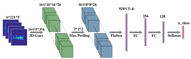
卷积神经网络 (CNN) 有助于理解图像、视频和音频方面的最新进展。一些工作（Zhao等人，2018；Zheng等人，2019；Jiang等人，2020）利用CNN在无线传感任务中进行无线信号理解，并取得了可喜的性能。本节将提供一个工作示例来演示如何将 CNN 应用于无线传感。具体来说，我们使用商用 Wi-Fi 来识别六种人类手势。手势如图9所示。我们在一个典型的教室中部署了一个 Wi-Fi 发射器和六个接收器，设备设置如图10所示。用户被要求在五个标记位置和五个方向上执行手势。数据样本可以在我们发布的数据集（Yang等人，2020）中找到。我们从原始 CSI 信号中提取 DFS，并将其输入 CNN 网络。网络架构如图11所示。

现在我们详细介绍一下实现代码。

首先导入一些必要的包。我们使用 Keras (Chollet 等人, 2015) API 和 TensorFlow 作为后端来演示如何实现神经网络。

⬇

import os,sys

import numpy as np

import scipy.io as scio

import tensorflow as tf

import keras

from keras.layers import Input, GRU, Dense, Flatten, Dropout, Conv2D, Conv3D, MaxPooling2D, MaxPooling3D, TimeDistributed, Bidirectional, Multiply, Permute, RepeatVector, Concatenate, Dot, Lambda

from keras.models import Model, load_model

import keras.backend as K

from sklearn.metrics import confusion_matrix

from keras.backend.tensorflow_backend import set_session

from sklearn.model_selection import train_test_split

然后我们定义一些参数，包括超参数和数据路径。测试数据的分数定义为0.1。为了简化问题，我们只使用 widar3.0 数据集中的六种手势类型。

⬇

# Parameters

fraction_for_test = 0.1

data_dir = ’widar30dataset/DFS/20181130/’

ALL_MOTION = [1,2,3,4,5,6]

N_MOTION = len(ALL_MOTION)

T_MAX = 0

n_epochs = 200

f_dropout_ratio = 0.5

n_gru_hidden_units = 64

n_batch_size = 32

f_learning_rate = 0.001

该程序首先使用预定义函数load_data加载数据。通过调用API函数train_test_split将加载的数据分为训练和测试。使用预定义函数 onehot_encoding 将训练数据的标签编码为 one-hot 格式。

⬇

# Load data

data, label = load_data(data_dir)

print(’\nLoaded dataset of ’ + str(label.shape[0]) + ’ samples, each sized ’ + str(data[0,:,:,:,:].shape) + ’\n’)

# Split train and test

[data_train, data_test, label_train, label_test] = train_test_split(data, label, test_size=fraction_for_test)

print(’\nTrain on ’ + str(label_train.shape[0]) + ’ samples\n’ +\

’Test on ’ + str(label_test.shape[0]) + ’ samples\n’)

# One-hot encoding for train data

label_train = onehot_encoding(label_train, N_MOTION)

加载并格式化训练和测试数据后，我们使用预定义函数 build_model 定义模型。之后，我们通过调用API函数fit来训练模型。输入数据和标签在参数中指定。验证数据的分数指定为 0.1。

⬇

# Train Model

model = build_model(input_shape=(T_MAX, 6, 121, 1), n_class=N_MOTION)

model.summary()

model.fit({’name_model_input’: data_train},{’name_model_output’: label_train},

batch_size=n_batch_size,

epochs=n_epochs,

verbose=1,

validation_split=0.1, shuffle=True)

训练过程结束后，我们使用测试数据集评估模型。预测从 one-hot 格式转换为整数，并用于计算混淆矩阵和准确性。

⬇

# Testing...

print(’Testing...’)

label_test_pred = model.predict(data_test)

label_test_pred = np.argmax(label_test_pred, axis = -1) + 1

# Confusion Matrix

cm = confusion_matrix(label_test, label_test_pred)

print(cm)

cm = cm.astype(’float’)/cm.sum(axis=1)[:, np.newaxis]

cm = np.around(cm, decimals=2)

print(cm)

# Accuracy

test_accuracy = np.sum(label_test == label_test_pred) / (label_test.shape[0])

print(test_accuracy)

预定义的 onehot_encoding 函数将标签转换为 one-hot 格式。

⬇

def onehot_encoding(label, num_class):

# label(ndarray)=>_label(ndarray): [N,]=>[N,num_class]

label = np.array(label).astype(’int32’)

label = np.squeeze(label)

_label = np.eye(num_class)[label-1]

return _label

预定义的load_data函数用于从目录加载所有数据样本和标签。目录中的每个文件对应一个数据样本。每个数据样本都使用预定义的 normalize_data 函数进行标准化。值得注意的是，数据样本具有不同的持续时间。我们使用预定义的 zero_padding 函数来使它们的持续时间与最长的持续时间相同。

⬇

def load_data(path_to_data):

global T_MAX

data = []

label = []

for data_root, data_dirs, data_files in os.walk(path_to_data):

for data_file_name in data_files:

file_path = os.path.join(data_root,data_file_name)

try:

data_1 = scio.loadmat(file_path)[’doppler_spectrum’] # [6,121,T]

label_1 = int(data_file_name.split(’-’)[1])

location = int(data_file_name.split(’-’)[2])

orientation = int(data_file_name.split(’-’)[3])

repetition = int(data_file_name.split(’-’)[4])

# Downsample

data_1 = data_1[:,:,0::10]

# Select Motion

if (label_1 not in ALL_MOTION):

continue

# Normalization

data_normed_1 = normalize_data(data_1)

# Update T_MAX

if T_MAX < np.array(data_1).shape[2]:

T_MAX = np.array(data_1).shape[2]

except Exception:

continue

# Save List

data.append(data_normed_1.tolist())

label.append(label_1)

# Zero-padding

data = zero_padding(data, T_MAX)

# Swap axes

data = np.swapaxes(np.swapaxes(data, 1, 3), 2, 3) # [N,6,121,T_MAX]=>[N,T_MAX,6,121]

data = np.expand_dims(data, axis=-1) # [N,T_MAX,6,121]=>[N,T_MAX,6,121,1]

# Convert label to ndarray

label = np.array(label)

# data(ndarray): [N,T_MAX,6,121,1], label(ndarray): [N,]

return data, label

normalize_data 函数用于对加载的数据样本进行标准化。每个数据样本的维度为 $[6,121,T]$ ，其中数字“6”代表Wi-Fi接收器的数量，数字“121”代表频率仓，“T”代表持续时间。为了标准化样本，我们将每个时间快照的数据缩放到 $[0,1]$ 范围内。

⬇

def normalize_data(data_1):

# data(ndarray)=>data_norm(ndarray): [6,121,T]=>[6,121,T]

data_1_max = np.amax(data_1,(0,1),keepdims=True) # [6,121,T]=>[1,1,T]

data_1_min = np.amin(data_1,(0,1),keepdims=True) # [6,121,T]=>[1,1,T]

data_1_max_rep = np.tile(data_1_max,(data_1.shape[0],data_1.shape[1],1)) # [1,1,T]=>[6,121,T]

data_1_min_rep = np.tile(data_1_min,(data_1.shape[0],data_1.shape[1],1)) # [1,1,T]=>[6,121,T]

data_1_norm = (data_1 - data_1_min_rep) / (data_1_max_rep - data_1_min_rep + sys.float_info.min)

return data_1_norm

zero_padding 函数用于将所有数据样本对齐以具有相同的持续时间。填充长度由参数T_MAX指定。

⬇

def zero_padding(data, T_MAX):

# data(list)=>data_pad(ndarray): [6,121,T1/T2/...]=>[6,121,T_MAX]

data_pad = []

for i in range(len(data)):

t = np.array(data[i]).shape[2]

data_pad.append(np.pad(data[i], ((0,0),(0,0),(T_MAX - t,0)), ’constant’, constant_values = 0).tolist())

return np.array(data_pad)

在这个函数中，我们定义了网络结构。输入层通过 API 函数 Input 指定，该函数具有定义输入形状、数据类型和层名称的参数。在输入层之后，我们使用三维卷积层、最大池层和两个全连接层。输出层由 API 函数 Output 指定，该函数具有定义激活函数、维度和名称的参数。最后，我们使用 API 函数 Model 和 compile 完成模型。优化器指定为RMSprop，损失指定为categorical_crossentropy。

⬇

def build_model(input_shape, n_class):

model_input = Input(shape=input_shape, dtype=’float32’, name=’name_model_input’) # (@,T_MAX,6,121,1)

# CNN

x = Conv3D(16,kernel_size=(5,3,6),activation=’relu’,data_format=’channels_last’,\

input_shape=input_shape)(model_input) # (@,T_MAX-4,6,121,1)=>(@,T_MAX-4,4,116,16)

x = MaxPooling3D(pool_size=(2,2,2))(x) # (@,T_MAX-4,4,116,16)=>(@,T_MAX-4,2,58,16)

x = Flatten()(x) # (@,T_MAX-4,2,58,16)=>(@,(T_MAX-4)*2*58*16)

x = Dense(256,activation=’relu’)(x) # (@,(T_MAX-4)*2*58*16)=>(@,256)

x = Dropout(f_dropout_ratio)(x)

x = Dense(128,activation=’relu’)(x) # (@,256)=>(@,128)

x = Dropout(f_dropout_ratio)(x)

model_output = Dense(n_class, activation=’softmax’, name=’name_model_output’)(x) # (@,128)=>(@,n_class)

# Model compiling

model = Model(inputs=model_input, outputs=model_output)

model.compile(optimizer=keras.optimizers.RMSprop(lr=f_learning_rate),

loss=’categorical_crossentropy’,

metrics=[’accuracy’]

)

return model

6.2. 循环神经网络

递归神经网络 (RNN) 旨在对序列的时间动态进行建模，通常用于语音识别和自然语言处理等时间序列数据分析。无线信号随时间高度相关，可以使用 RNN 进行处理。一些工作（Zheng等人，2019；Jiang等人，2020）展示了RNN在无线传感任务中的潜力。在本节中，我们将展示一个结合 CNN 和 RNN 通过 Wi-Fi 执行手势识别的工作示例。实验设置与第 2 节中的相同。 6.1。我们还从原始 CSI 中提取 DFS 作为网络的输入特征。网络架构如图12所示。

现在我们详细介绍一下实现代码。

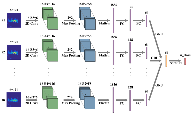
大部分代码与第 2 节中的相同。 6.1 除了模型定义。为了定义模型，我们在数据的时间维度之外的维度上使用二维卷积层和最大池化层。我们采用 GRU 层作为循环层。

⬇

def build_model(input_shape, n_class):

model_input = Input(shape=input_shape, dtype=’float32’, name=’name_model_input’) # (@,T_MAX,6,121,1)

# CNN+RNN

x = TimeDistributed(Conv2D(16,kernel_size=(3,6),activation=’relu’,data_format=’channels_last’,\

input_shape=input_shape))(model_input) # (@,T_MAX,6,121,1)=>(@,T_MAX,4,116,16)

x = TimeDistributed(MaxPooling2D(pool_size=(2,2)))(x) # (@,T_MAX,4,116,16)=>(@,T_MAX,2,58,16)

x = TimeDistributed(Flatten())(x) # (@,T_MAX,2,58,16)=>(@,T_MAX,2*58*16)

x = TimeDistributed(Dense(128,activation=’relu’))(x) # (@,T_MAX,2*58*16)=>(@,T_MAX,128)

x = TimeDistributed(Dropout(f_dropout_ratio))(x)

x = TimeDistributed(Dense(64,activation=’relu’))(x) # (@,T_MAX,128)=>(@,T_MAX,64)

x = GRU(n_gru_hidden_units,return_sequences=False)(x) # (@,T_MAX,64)=>(@,64)

x = Dropout(f_dropout_ratio)(x)

model_output = Dense(n_class, activation=’softmax’, name=’name_model_output’)(x) # (@,64)=>(@,n_class)

# Model compiling

model = Model(inputs=model_input, outputs=model_output)

model.compile(optimizer=keras.optimizers.RMSprop(lr=f_learning_rate),

loss=’categorical_crossentropy’,

metrics=[’accuracy’]

)

return model

6.3. 对抗性学习

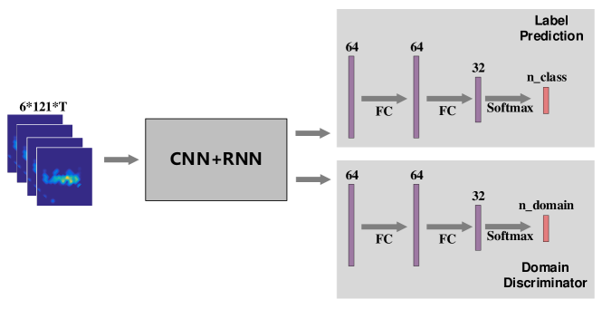
除了基本的神经网络组件之外，一些高级网络架构在无线传感中也发挥着重要作用。与计算机视觉任务类似，无线传感也面临域错位问题。无线信号在传播过程中可能会被周围物体反射，并且会充斥着与目标无关的信号分量。在一种部署环境中训练的传感系统很难在不进行适应的情况下直接应用于其他环境。一些作品（Jiang等人，2018）尝试采用对抗性学习技术来解决这个问题并取得了可喜的性能。本节将举例说明如何在无线传感任务中应用该技术。具体来说，我们使用 Wi-Fi 构建了一个手势识别系统，类似于第 2 节中的系统。 6.1。我们尝试在不同的人员位置和方向上实现一致的性能。网络架构如图13所示。

现在我们详细介绍一下实现代码。

在Widar3.0数据集（Yang等人，2020）中，我们收集用户站在不同位置时的手势数据。正如第 2 节中所讨论的。 4.3，人体位置对DFS测量有显着影响。为了减轻这种影响，我们将人类位置视为不同的领域，并构建一个对抗性学习网络来识别手势，而不管领域如何。在程序中，我们首先从数据集中加载数据、标签和域，并将它们拆分为训练和测试。标签和域都被编码为 one-hot 格式。

⬇

# Load data

data, label, domain = load_data(data_dir)

print(’\nLoaded dataset of ’ + str(label.shape[0]) + ’ samples, each sized ’ + str(data[0,:,:,:,:].shape) + ’\n’)

# Split train and test

[data_train, data_test, label_train, label_test, domain_train, domain_test] = train_test_split(data, label, domain, test_size=fraction_for_test)

print(’\nTrain on ’ + str(label_train.shape[0]) + ’ samples\n’ +\

’Test on ’ + str(label_test.shape[0]) + ’ samples\n’)

# One-hot encoding for train data

label_train = onehot_encoding(label_train, N_MOTION)

domain_train = onehot_encoding(domain_train, N_LOCATION)

加载和格式化数据后，我们构建了网络并从头开始训练它。训练数据、标签和域被传递给 API 函数 fit 进行训练。

⬇

# Train Model

model = build_model(input_shape=(T_MAX, 6, 121, 1), n_class=N_MOTION, n_domain=N_LOCATION)

model.summary()

model.fit({’name_model_input’: data_train},{’name_model_output_label’: label_train, ’name_model_output_domain’: domain_train},

batch_size=n_batch_size,

epochs=n_epochs,

verbose=1,

validation_split=0.1, shuffle=True)

训练过程完成后，我们用测试样本评估网络。请注意，对抗网络具有标签和域预测输出。我们仅使用标签输出来进行准确性评估。

⬇

# Testing...

print(’Testing...’)

[label_test_pred,_] = model.predict(data_test)

label_test_pred = np.argmax(label_test_pred, axis = -1) + 1

# Confusion Matrix

cm = confusion_matrix(label_test, label_test_pred)

print(cm)

cm = cm.astype(’float’)/cm.sum(axis=1)[:, np.newaxis]

cm = np.around(cm, decimals=2)

print(cm)

# Accuracy

test_accuracy = np.sum(label_test == label_test_pred) / (label_test.shape[0])

print(test_accuracy)

与第二节不同。 6.1，我们在load_data函数中加载数据、标签和域。域被定义为嵌入在文件名中的人类位置。

⬇

def load_data(path_to_data):

global T_MAX

data = []

label = []

domain = []

for data_root, data_dirs, data_files in os.walk(path_to_data):

for data_file_name in data_files:

file_path = os.path.join(data_root,data_file_name)

try:

data_1 = scio.loadmat(file_path)[’doppler_spectrum’] # [6,121,T]

label_1 = int(data_file_name.split(’-’)[1])

location_1 = int(data_file_name.split(’-’)[2])

orientation_1 = int(data_file_name.split(’-’)[3])

repetition_1 = int(data_file_name.split(’-’)[4])

# Downsample

data_1 = data_1[:,:,0::10]

# Select Motion

if (label_1 not in ALL_MOTION):

continue

# Normalization

data_normed_1 = normalize_data(data_1)

# Update T_MAX

if T_MAX < np.array(data_1).shape[2]:

T_MAX = np.array(data_1).shape[2]

except Exception:

continue

# Save List

data.append(data_normed_1.tolist())

label.append(label_1)

domain.append(location_1)

# Zero-padding

data = zero_padding(data, T_MAX)

# Swap axes

data = np.swapaxes(np.swapaxes(data, 1, 3), 2, 3) # [N,6,121,T_MAX]=>[N,T_MAX,6,121]

data = np.expand_dims(data, axis=-1) # [N,T_MAX,6,121]=>[N,T_MAX,6,121,1]

# Convert label and domain to ndarray

label = np.array(label)

domain = np.array(domain)

# data(ndarray): [N,T_MAX,6,121,1], label(ndarray): [N,], domain(ndarray): [N,]

return data, label, domain

为了定义网络，我们使用 CNN 层和 RNN 层作为特征提取器，这与第 2 节中的类似。 6.2。在手势识别器和域鉴别器中，我们分别使用两个全连接层和一个由 softmax 函数激活的输出层。我们对标签预测和域预测输出使用分类交叉熵损失。域预测损失用 loss_weight_domain 进行加权，并从标签预测损失中减去。

⬇

def build_model(input_shape, n_class, n_domain):

model_input = Input(shape=input_shape, dtype=’float32’, name=’name_model_input’) # (@,T_MAX,6,121,1)

# CNN+RNN+Adversarial

x = TimeDistributed(Conv2D(16,kernel_size=(3,6),activation=’relu’,data_format=’channels_last’,\

input_shape=input_shape))(model_input) # (@,T_MAX,6,121,1)=>(@,T_MAX,4,116,16)

x = TimeDistributed(MaxPooling2D(pool_size=(2,2)))(x) # (@,T_MAX,4,116,16)=>(@,T_MAX,2,58,16)

x = TimeDistributed(Flatten())(x) # (@,T_MAX,2,58,16)=>(@,T_MAX,2*58*16)

x = TimeDistributed(Dense(128,activation=’relu’))(x) # (@,T_MAX,2*58*16)=>(@,T_MAX,128)

x = TimeDistributed(Dropout(f_dropout_ratio))(x)

x = TimeDistributed(Dense(64,activation=’relu’))(x) # (@,T_MAX,128)=>(@,T_MAX,64)

x = GRU(n_gru_hidden_units,return_sequences=False)(x) # (@,T_MAX,64)=>(@,64)

x_feat = Dropout(f_dropout_ratio)(x)

# Label prediction part

x_1 = Dense(64, activation=’relu’)(x_feat) # (@,64)=>(@,64)

x_1 = Dense(32, activation=’relu’)(x_1) # (@,64)=>(@,32)

model_output_label = Dense(n_class, activation=’softmax’, name=’name_model_output_label’)(x_1) # (@,32)=>(@,n_class)

# Domain prediction part

x_2 = Dense(64, activation=’relu’)(x_feat) # (@,64)=>(@,64)

x_2 = Dense(32, activation=’relu’)(x_2) # (@,64)=>(@,32)

model_output_domain = Dense(n_domain, activation=’softmax’, name=’name_model_output_domain’)(x_2) # (@,32)=>(@,n_domain)

model = Model(inputs=model_input, outputs=[model_output_label, model_output_domain])

model.compile(optimizer=keras.optimizers.RMSprop(lr=f_learning_rate),

loss = {’name_model_output_label’:custom_loss_label(), ’name_model_output_domain’:custom_loss_domain()},

loss_weights={’name_model_output_label’:1, ’name_model_output_domain’:-1*loss_weight_domain},

metrics={’name_model_output_label’:’accuracy’, ’name_model_output_domain’:’accuracy’}

)

return model

预定义的 custom_loss_label 和 custom_loss_domain 是标签预测和域预测的分类交叉熵损失。

⬇

def custom_loss_label():

def lossfn(y_true, y_pred):

myloss_batch = -1 * K.sum(y_true*K.log(y_pred+K.epsilon()), axis=-1, keepdims=False)

myloss = K.mean(myloss_batch, axis=-1, keepdims=False)

return myloss

return lossfn

⬇

def custom_loss_domain():

def lossfn(y_true, y_pred):

myloss_batch = -1 * K.sum(y_true*K.log(y_pred+K.epsilon()), axis=-1, keepdims=False)

myloss = K.mean(myloss_batch, axis=-1, keepdims=False)

return myloss

return lossfn

6.4. 复值神经网络

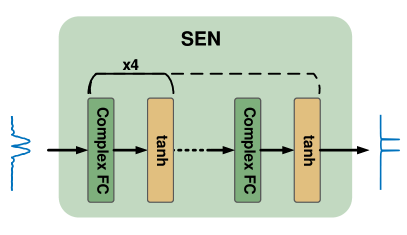
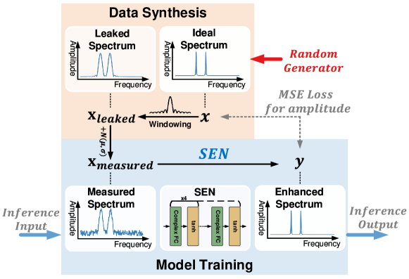
在本节中，我们将通过深度学习提出更复杂的无线传感任务。许多无线传感方法对射频数据的时间序列采用快速傅立叶变换 (FFT)，以获得人类活动的时频频谱图。当数据块不是周期性的（实践中最常见的情况）时，FFT 会因泄漏效应而出现错误，这会导致原始信号的频谱模糊，并进一步导致基于学习的数据表示误导传感。经典方法通过加窗来减少泄漏，但这不能完全消除泄漏。考虑到深度神经网络显着的拟合能力，我们可以设计一个信号处理网络来学习最优函数，以最小化或几乎消除泄漏并增强频谱，我们将其称为信号增强网络（SEN）。

信号处理网络将通过 STFT 从无线信号转换而来的频谱图作为输入，消除频谱图中的频谱泄漏，并恢复底层的实际频率分量。图16展示了网络的训练过程。如图16上半部分所示，我们随机生成具有1到5个频率分量的理想频谱，其幅度、相位和频率统一从其感兴趣的范围中抽取。然后，按照以下方程的过程将理想频谱转换为泄漏频谱，以模拟加窗效应和随机复噪声：

(34)

\hat{\mathbf{s}}=\mathbf{A}\mathbf{s}+\mathbf{n},

其中 $\mathbf{s}$ 和 $\hat{\mathbf{s}}$ 分别是理想频谱和估计频谱， $\mathbf{n}$ 表示加性高斯噪声向量， $\mathbf{A}$ 是频域加窗函数的卷积矩阵。 $\mathbf{A}$ 的 $i^{th}$ 列是：

(35)

\mathbf{A_{(:,i)}}={\rm FFT}(\mathbf{\varpi})*\delta(i).

其中 $\mathbf{\varpi}$ 表示时域FFT的加窗函数。

噪声的幅度服从高斯分布，其相位服从 $[0,2\pi]$ 中的均匀分布。该网络将泄漏的频谱作为输入，并输出接近理想频谱的增强频谱。因此，我们可以最大限度地减少训练期间的 $L_{2}$ 损失 $L=||{\rm SEN}(\hat{\mathbf{s}})-\mathbf{s}||_{2}$ 。在推理过程中，从现实场景中测量的频谱被归一化为 $[0,1]$ 并馈入网络以获得增强的频谱。

现在我们详细介绍一下实现代码。

与前面几节不同的是，我们使用PyTorch平台来实现网络。 PyTorch提供了实现自定义层的接口，这使得CVNN的实现更加方便。我们首先导入一些必要的包，如下所示。

⬇

import os,sys,math,scipy,imp

import numpy as np

import scipy.io as scio

import torch, torchvision

import torch.nn as nn

from scipy import signal

from math import sqrt,log,pi

from torch.fft import fft,ifft

from torch.nn.functional import relu, softmax, cross_entropy

from torch import sigmoid,tanh

from torch.nn import MSELoss as MSE

本部分定义了一些参数。

⬇

# Definition

wind_len = 125

wind_type = ’gaussian’

n_max_freq_component = 3

AWGN_amp = 0.01

str_modelname_prefix = ’./SEN_Results/SEN_’ + wind_type + ’_W’ + str(wind_len)

str_model_name_pretrained = str_modelname_prefix + ’_E1000.pt’

feature_len = 121

padded_len = 1000

crop_len = feature_len

blur_matrix_left = []

# Hyperparameters

n_begin_epoch = 1

n_epoch = 10000

n_itr_per_epoch = 500

n_batch_size = 64

n_test_size = 200

f_learning_rate = 0.001

该程序以以下代码开始。我们首先生成加窗函数的卷积矩阵（方程： 35)与预定义函数generate_blur_matrix_complex，该函数很快就会介绍。然后我们定义SEN模型并使用API函数cuda将其移动到GPU处理器。模型定义后，我们使用合成频谱图训练模型，在此过程中，我们每 500 个时期保存训练后的模型。训练和保存的模型可以直接加载并用于增强频谱图。

⬇

if __name__ == "__main__":

# Generate blur matrix

blur_matrix_right = generate_blur_matrix_complex(wind_type=wind_type, wind_len=wind_len, padded_len=padded_len, crop_len=crop_len)

# Define model

print(’Model building...’)

model = SEN(feature_len=feature_len)

model.cuda()

# Train model

print(’Model training...’)

train(model=model, blur_matrix_right=blur_matrix_right, feature_len=feature_len, n_epoch=n_epoch, n_itr_per_epoch=n_itr_per_epoch, n_batch_size=n_batch_size, optimizer=torch.optim.RMSprop(model.parameters(), lr=f_learning_rate))

这个generate_blur_matrix_complex函数用于生成加窗函数的卷积矩阵。该函数背后的核心思想是枚举所有频率，对正弦信号应用窗函数，并通过 FFT 生成相应的频谱。获得卷积矩阵后，我们可以用方程（1）弥补理想谱图和泄漏谱图之间的差距。 34. 换句话说，我们可以通过将想法谱图与卷积矩阵相乘来直接得到泄漏的谱图。

⬇

def generate_blur_matrix_complex(wind_type, wind_len=251, padded_len=1000, crop_len=121):

# Generate matrix used to introduce spec leakage in complex domain

# ret: (ndarray.complex128) [crop_len, crop_len](row first)

# Row first: each row represents the spectrum of one single carrier

# Steps: carrier/windowing/pad/fft/crop/unwrap/norm

# Parameters offloading

fs = 1000

n_f_bins = crop_len

f_high = int(n_f_bins/2)

f_low = -1 * f_high

init_phase = 0

# Carrier

t_ = np.arange(0,wind_len).reshape(1,wind_len)/fs # [1,wind_len] (0~wind_len/fs seconds)

freq = np.arange(f_low,f_high+1,1).reshape(n_f_bins,1) # [n_f_bins,1] (f_low~f_high Hz)

phase = 2 * pi * freq * t_ + init_phase # [n_f_bins,wind_len]

signal = np.exp(1j*phase) # [n_f_bins,wind_len]~[121,251]

# Windowing

if wind_type == ’gaussian’:

window = scipy.signal.windows.gaussian(wind_len, (wind_len-1)/sqrt(8*log(200)), sym=True) # [wind_len,]

else:

window = scipy.signal.get_window(wind_type, wind_len)

sig_wind = signal * window # [n_f_bins,wind_len]*[wind_len,]=[n_f_bins,wind_len]~[121,251]

# Pad/FFT

sig_wind_pad = np.concatenate((sig_wind, np.zeros((n_f_bins,padded_len-wind_len))),axis=1) # [n_f_bins,wind_len]=>[n_f_bins,padded_len]

sig_wind_pad_fft = np.fft.fft(sig_wind_pad, axis=-1) # [n_f_bins,padded_len]~[121,1000]

# Crop

n_freq_pos = f_high + 1

n_freq_neg = abs(f_low)

sig_wind_pad_fft_crop = np.concatenate((sig_wind_pad_fft[:,:n_freq_pos],\

sig_wind_pad_fft[:,-1*n_freq_neg:]), axis=1) # [n_f_bins,crop_len]~[121,121]

# Unwrap

n_shift = n_freq_neg

sig_wind_pad_fft_crop_unwrap = np.roll(sig_wind_pad_fft_crop, shift=n_shift, axis=1) # [n_f_bins,crop_len]~[121,121]

# Norm (amp_max=1)

_sig_amp = np.abs(sig_wind_pad_fft_crop_unwrap)

_sig_ang = np.angle(sig_wind_pad_fft_crop_unwrap)

_max = np.tile(_sig_amp.max(axis=1,keepdims=True), (1,crop_len))

_min = np.tile(_sig_amp.min(axis=1,keepdims=True), (1,crop_len))

_sig_amp_norm = _sig_amp / _max

sig_wind_pad_fft_crop_unwrap_norm = _sig_amp_norm * np.exp(1j*_sig_ang)

# Return

ret = sig_wind_pad_fft_crop_unwrap_norm

return ret

该功能是生成一批泄漏形式和想法形式的频谱图。该过程与方程式中所示的相同。 34.

⬇

def syn_one_batch_complex(blur_matrix_right, feature_len, n_batch):

# Syn. HiFi, blurred and AWGN signal in complex domain

# ret: (ndarray.complex128) [@,feature_len]

# blur_matrix_right: Row first (each row represents the spectrum of one single carrier)

# Syn. x [@,feature_len]

x = np.zeros((n_batch, feature_len))*np.exp(1j*0)

for i in range(n_batch):

num_carrier = int(np.random.randint(0,n_max_freq_component,1))

idx_carrier = np.random.permutation(feature_len)[:num_carrier]

x[i,idx_carrier] = np.random.rand(1,num_carrier) * np.exp(1j*( 2*pi*np.random.rand(1,num_carrier) - pi ))

# Syn. x_blur [@,feature_len]

x_blur = x @ blur_matrix_right

# Syn. x_tilde [@,feature_len]

x_tilde = x_blur + 2*AWGN_amp*(np.random.random(x_blur.shape)-0.5) *\

np.exp(1j*( 2*pi*np.random.random(x_blur.shape) - pi ))

return x, x_blur, x_tilde

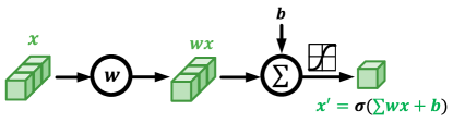
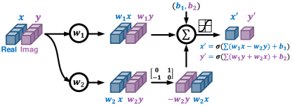
这部分演示了如何实现SEN网络的代码。根据PyTorch的API，__init__和forward接口都应该使用自定义算法来实现。在__init__函数中，我们定义了五个复值全连接层。在forward函数中，我们通过连接五个FC层并指定输入和输出层来定义网络结构。

⬇

class SEN(nn.Module):

def __init__(self, feature_len):

super(SEN, self).__init__()

self.feature_len = feature_len

self.fc_1 = m_Linear(feature_len, feature_len)

self.fc_2 = m_Linear(feature_len, feature_len)

self.fc_3 = m_Linear(feature_len, feature_len)

self.fc_4 = m_Linear(feature_len, feature_len)

self.fc_out = m_Linear(feature_len, feature_len)

def forward(self, x):

h = x # (@,*,2,H)

h = tanh(self.fc_1(h)) # (@,*,2,H)=>(@,*,2,H)

h = tanh(self.fc_2(h)) # (@,*,2,H)=>(@,*,2,H)

h = tanh(self.fc_3(h)) # (@,*,2,H)=>(@,*,2,H)

h = tanh(self.fc_4(h)) # (@,*,2,H)=>(@,*,2,H)

output = tanh(self.fc_out(h)) # (@,*,2,H)=>(@,*,2,H)

return output

这个m_Linear类利用PyTorch的接口来定义定制的复值全连接层，它是图14所示网络结构的实现。

⬇

class m_Linear(nn.Module):

def __init__(self, size_in, size_out):

super().__init__()

self.size_in, self.size_out = size_in, size_out

# Creation

self.weights_real = nn.Parameter(torch.randn(size_in, size_out, dtype=torch.float32))

self.weights_imag = nn.Parameter(torch.randn(size_in, size_out, dtype=torch.float32))

self.bias = nn.Parameter(torch.randn(2, size_out, dtype=torch.float32))

# Initialization

nn.init.xavier_uniform_(self.weights_real, gain=1)

nn.init.xavier_uniform_(self.weights_imag, gain=1)

nn.init.zeros_(self.bias)

def swap_real_imag(self, x):

# [@,*,2,Hout]

# [real, imag] => [-1*imag, real]

h = x # [@,*,2,Hout]

h = h.flip(dims=[-2]) # [@,*,2,Hout] [real, imag]=>[imag, real]

h = h.transpose(-2,-1) # [@,*,Hout,2]

h = h * torch.tensor([-1,1]).cuda() # [@,*,Hout,2] [imag, real]=>[-1*imag, real]

h = h.transpose(-2,-1) # [@,*,2,Hout]

return h

def forward(self, x):

# x: [@,*,2,Hin]

h = x # [@,*,2,Hin]

h1 = torch.matmul(h, self.weights_real) # [@,*,2,Hout]

h2 = torch.matmul(h, self.weights_imag) # [@,*,2,Hout]

h2 = self.swap_real_imag(h2) # [@,*,2,Hout]

h = h1 + h2 # [@,*,2,Hout]

h = torch.add(h, self.bias) # [@,*,2,Hout]+[2,Hout]=>[@,*,2,Hout]

return h

这个loss_function定义了SEN网络的损失函数。损失被定义为想法谱与网络预测谱之间的欧几里德距离。仅考虑频谱的幅度。

⬇

def loss_function(x, y):

# x,y: [@,*,2,H]

x = torch.linalg.norm(x,dim=-2) # [@,*,2,H]=>[@,*,H]

y = torch.linalg.norm(y,dim=-2) # [@,*,2,H]=>[@,*,H]

# MSE loss for Amp

loss_recon = MSE(reduction=’mean’)(x, y)

return loss_recon

在这个训练函数中，我们实现了如图16所示的SEN训练过程。在每个时期，我们都会通过多次迭代来生成和训练网络。对于每次迭代，我们都会生成一批泄漏格式的合成光谱。每个泄露的频谱都有一个想法频谱作为标签。

⬇

def train(model, blur_matrix_right, feature_len, n_epoch, n_itr_per_epoch, n_batch_size, optimizer):

for i_epoch in range(n_begin_epoch, n_epoch+1):

model.train()

total_loss_this_epoch = 0

for i_itr in range(n_itr_per_epoch):

x, _, x_tilde = syn_one_batch_complex(blur_matrix_right=blur_matrix_right, feature_len=feature_len, n_batch=n_batch_size)

x = complex_array_to_bichannel_float_tensor(x)

x_tilde = complex_array_to_bichannel_float_tensor(x_tilde)

x = x.cuda()

x_tilde = x_tilde.cuda()

optimizer.zero_grad()

y = model(x_tilde)

loss = loss_function(x, y)

loss.backward()

optimizer.step()

total_loss_this_epoch += loss.item()

if i_itr % 10 == 0:

print(’--------> Epoch: {}/{} loss: {:.4f} [itr: {}/{}]’.format(

i_epoch+1, n_epoch, loss.item() / n_batch_size, i_itr+1, n_itr_per_epoch), end=’\r’)

# Validate

model.eval()

x, _, x_tilde = syn_one_batch_complex(blur_matrix_right=blur_matrix_right, feature_len=feature_len, n_batch=n_batch_size)

x = complex_array_to_bichannel_float_tensor(x)

x_tilde = complex_array_to_bichannel_float_tensor(x_tilde)

x = x.cuda()

x_tilde = x_tilde.cuda()

y = model(x_tilde)

total_valid_loss = loss_function(x, y)

print(’========> Epoch: {}/{} Loss: {:.4f}’.format(i_epoch+1, n_epoch, total_valid_loss) + ’ ’ + wind_type + ’_’ + str(wind_len) + ’ ’*20)

if i_epoch % 500 == 0:

torch.save(model, str_modelname_prefix+’_E’+str(i_epoch)+’.pt’)

该函数将复值数组转换为双通道实值数组。这是因为GPU只支持实数的计算。我们使用一个小技巧，通过将实部和虚部分成两个实数数组来实现复值网络。

⬇

def complex_array_to_bichannel_float_tensor(x):

# x: (ndarray.complex128) [@,*,H]

# ret: (tensor.float32) [@,*,2,H]

x = x.astype(’complex64’)

x_real = x.real # [@,*,H]

x_imag = x.imag # [@,*,H]

ret = np.stack((x_real,x_imag), axis=-2) # [@,*,H]=>[@,*,2,H]

ret = torch.tensor(ret)

return ret

该函数将双通道实值数组转换为复值数组。

⬇

def bichannel_float_tensor_to_complex_array(x):

# x: (tensor.float32) [@,*,2,H]

# ret: (ndarray.complex64) [@,*,H]

x = x.numpy()

x = np.moveaxis(x,-2,0) # [@,*,2,H]=>[2,@,*,H]

x_real = x[0,:]

x_imag = x[1,:]

ret = x_real + 1j*x_imag

return ret

在使用足够的 epoch 训练 SEN 网络后，我们使用从 Wi-Fi 收集的频谱图来测试性能。

首先，我们定义一些参数。 STFT窗口宽度设置为125，窗口类型设置为“高斯”。选择预训练模型和 CSI 文件的路径。

⬇

W = 125

wind_type = ’gaussian’

str_model_name = ’./SEN_Results/SEN_’ + wind_type + ’_W’ + str(W) + ’_E500.pt’

file_path_csi = ’Widar3_data/20181130/user1/user1-1-1-1-1.mat’

该程序首先加载预先训练的模型。然后，使用预定义函数csi_to_spec加载CSI数据并将其转换为频谱图。之后，将复值频谱图转换为双实值通道张量并使用 SEN 模型进行处理。结果和原始频谱图存储在文件中。

⬇

if __name__ == "__main__":

# Load trained model

print(’Loading model...’)

model = torch.load(str_model_name)

print(’Testing model...’)

model.eval()

with torch.no_grad():

# Import raw spectrogram

data_1 = csi_to_spec()

# Enhance spectrogram

x_tilde = complex_array_to_bichannel_float_tensor(data_1) # [6,121,T]=>[6,121,2,T]

x_tilde = x_tilde.permute(0,3,2,1) # [6,121,2,T]=>[6,T,2,121]

y = model(x_tilde.cuda()).cpu() # [6,T,2,121]

y = bichannel_float_tensor_to_complex_array(y) # [6,T,121]

y = np.transpose(y,(0,2,1)) # [6,T,121]=>[6,121,T]

scio.savemat(’SEN_test_x_tilde_complex_W’ + str(W) + ’.mat’, {’x_tilde’:data_1})

scio.savemat(’SEN_test_y_complex_W’ + str(W) + ’.mat’, {’y’:y})

该函数首先将 CSI 数据转换为频谱图，并裁剪 $[-60,60]$ Hz 之间的相关频率范围。然后，它解开频率仓并执行归一化。

⬇

def csi_to_spec():

global file_path_csi

global W

signal = scio.loadmat(file_path_csi)[’csi_mat’].transpose() # [6,T] complex

# STFT

_, spec = STFT(signal, fs=1000, stride=1, wind_wid=W, dft_wid=1000, window_type=’gaussian’) # [6,1000,T]j

# Crop

spec_crop = np.concatenate((spec[:,:61], spec[:,-60:]), axis=1) # [1,1000,T]j=>[1,121,T]j

# Unwrap

spec_crop_unwrap = np.roll(spec_crop, shift=60, axis=1) # [1,121,T]j

# Normalize

spec_crop_unwrap_norm = normalize_data(spec_crop_unwrap) # [6,121,T] complex

if np.sum(np.isnan(spec_crop_unwrap_norm)):

print(’>>>>>>>>> NaN detected!’)

ret = spec_crop_unwrap_norm

return ret

该函数使用 API 函数 scipy.signal.stft 将时域 CSI 数据转换为频域频谱图。

⬇

def STFT(signal, fs=1, stride=1, wind_wid=5, dft_wid=5, window_type=’gaussian’):

assert dft_wid >= wind_wid and wind_wid > 0 and stride <= wind_wid and stride > 0\

and isinstance(stride, int) and isinstance(wind_wid, int) and isinstance(dft_wid, int)\

and isinstance(fs, int) and fs > 0

if window_type == ’gaussian’:

window = scipy.signal.windows.gaussian(wind_wid, (wind_wid-1)/sqrt(8*log(200)), sym=True)

elif window_type == ’rect’:

window = np.ones((wind_wid,))

else:

window = scipy.signal.get_window(window_type, wind_wid)

f_bins, t_bins, stft_spectrum = scipy.signal.stft(x=signal, fs=fs, window=window, nperseg=wind_wid, noverlap=wind_wid-stride, nfft=dft_wid,\

axis=-1, detrend=False, return_onesided=False, boundary=’zeros’, padded=True)

return f_bins, stft_spectrum

此函数缩放频谱图以将值标准化为 $[0,1]$ 。

⬇

def normalize_data(data_1):

# max=1

# data(ndarray.complex)=>data_norm(ndarray.complex): [6,121,T]=>[6,121,T]

data_1_abs = abs(data_1)

data_1_max = data_1_abs.max(axis=(1,2),keepdims=True) # [6,121,T]=>[6,1,1]

data_1_max_rep = np.tile(data_1_max,(1,data_1_abs.shape[1],data_1_abs.shape[2])) # [6,1,1]=>[6,121,T]

data_1_norm = data_1 / data_1_max_rep

return data_1_norm

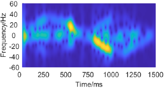
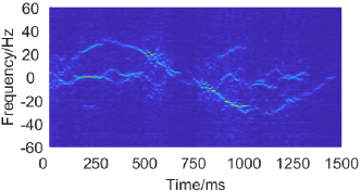
图17展示了推拉手势的原始频谱图和增强频谱图。

参考

(1)
Abdelnasser et al. (2015) Heba Abdelnasser, Moustafa Youssef, and Khaled A Harras. 2015. Wigest: A ubiquitous wifi-based gesture recognition system. In Proceedings of the IEEE INFOCOM.
Capon (1969) J. Capon. 1969. High-resolution frequency-wavenumber spectrum analysis. Proc. IEEE (1969).
Chi et al. (2021) Guoxuan Chi, Jingao Xu, Jialin Zhang, Qian Zhang, Qiang Ma, and Zheng Yang. 2021. Locate, Tell, and Guide: Enabling Public Cameras to Navigate the Public. IEEE Transactions on Mobile Computing (2021).
Chi et al. (2022) Guoxuan Chi, Zheng Yang, Jingao Xu, Chenshu Wu, Jialin Zhang, Jianzhe Liang, and Yunhao Liu. 2022. Wi-drone: Wi-Fi-based 6-DoF Tracking for Indoor Drone Flight Control. In Proceedings of the ACM MobiSys.
Chollet et al. (2015) François Chollet et al. 2015. Keras. https://github.com/fchollet/keras.
Donoho (2006) David L Donoho. 2006. Compressed sensing. IEEE Transactions on information theory (2006).
Halperin et al. (2011) Daniel Halperin, Wenjun Hu, Anmol Sheth, and David Wetherall. 2011. Tool release: Gathering 802.11 n traces with channel state information. ACM SIGCOMM computer communication review (2011).
Hill (2009) David A. Hill. 2009. Electromagnetic fields in cavities: deterministic and statistical theories. John Wiley & Sons (2009).
Hu et al. (2020) Yuqian Hu, Feng Zhang, Chenshu Wu, Beibei Wang, and K. J. Ray Liu. 2020. A WiFi-Based Passive Fall Detection System. In Proceedings of the IEEE ICASSP.
Jiang et al. (2018) Wenjun Jiang, Chenglin Miao, Fenglong Ma, Shuochao Yao, Yaqing Wang, Ye Yuan, Hongfei Xue, Chen Song, Xin Ma, Dimitrios Koutsonikolas, Wenyao Xu, and Lu Su. 2018. Towards Environment Independent Device Free Human Activity Recognition. In Proceedings of ACM MobiCom.
Jiang et al. (2020) Wenjun Jiang, Hongfei Xue, Chenglin Miao, Shiyang Wang, Sen Lin, Chong Tian, Srinivasan Murali, Haochen Hu, Zhi Sun, and Lu Su. 2020. Towards 3D Human Pose Construction Using Wifi. In Proceedings of the ACM MobiCom.
Jiang et al. (2021) Zhiping Jiang, Tom H Luan, Xincheng Ren, Dongtao Lv, Han Hao, Jing Wang, Kun Zhao, Wei Xi, Yueshen Xu, and Rui Li. 2021. Eliminating the Barriers: Demystifying Wi-Fi Baseband Design and Introducing the PicoScenes Wi-Fi Sensing Platform. IEEE Internet of Things Journal (2021).
Palipana et al. (2019) Sameera Palipana, David Rojas, Piyush Agrawal, and Dirk Pesch. 2019. FallDeFi: Ubiquitous Fall Detection Using Commodity Wi-Fi Devices. In Proceedings of the ACM IMWUT.
Patwari and Kasera (2007) Neal Patwari and Sneha K. Kasera. 2007. Robust Location Distinction Using Temporal Link Signatures. In Proceedings of the ACM MobiCom.
Qian et al. (2017) Kun Qian, Chenshu Wu, Zheng Yang, Yunhao Liu, and Kyle Jamieson. 2017. Widar: Decimeter-Level Passive Tracking via Velocity Monitoring with Commodity Wi-Fi. In Proceedings of the ACM MobiHoc.
Qian et al. (2014) Kun Qian, Chenshu Wu, Zheng Yang, Yunhao Liu, and Zimu Zhou. 2014. PADS: Passive detection of moving targets with dynamic speed using PHY layer information. In Proceedings of the IEEE ICPADS.
Qian et al. (2018) Kun Qian, Chenshu Wu, Yi Zhang, Guidong Zhang, Zheng Yang, and Yunhao Liu. 2018. Widar2.0: Passive human tracking with a single wi-fi link. Proceedings of the ACM MobiSys (2018).
Rubner and Tomasi (2001) Yossi Rubner and Carlo Tomasi. 2001. The earth mover’s distance. In Perceptual Metrics for Image Database Navigation. Springer.
Schmidt (1986) R. Schmidt. 1986. Multiple emitter location and signal parameter estimation. IEEE Transactions on Antennas and Propagation (1986).
Wang et al. (2016) Hao Wang, Daqing Zhang, Junyi Ma, Yasha Wang, Yuxiang Wang, Dan Wu, Tao Gu, and Bing Xie. 2016. Human Respiration Detection with Commodity Wifi Devices: Do User Location and Body Orientation Matter?. In Proceedings of the ACM Ubicomp.
Wu et al. (2015) Chenshu Wu, Zheng Yang, Zimu Zhou, Xuefeng Liu, Yunhao Liu, and Jiannong Cao. 2015. Non-Invasive Detection of Moving and Stationary Human With WiFi. IEEE Journal on Selected Areas in Communications (2015).
Wu et al. (2020) Chenshu Wu, Feng Zhang, Yuqian Hu, and K. J. Ray Liu. 2020. GaitWay: Monitoring and Recognizing Gait Speed Through the Walls. IEEE Transactions on Mobile Computing (2020).
Xie et al. (2018) Yaxiong Xie, Zhenjiang Li, and Mo Li. 2018. Precise power delay profiling with commodity Wi-Fi. IEEE Transactions on Mobile Computing (2018).
Xie et al. (2019) Yaxiong Xie, Jie Xiong, Mo Li, and Kyle Jamieson. 2019. mD-Track: Leveraging multi-dimensionality for passive indoor Wi-Fi tracking. In Proceedings of the ACM MobiCom.
Yang et al. (2020) Zheng Yang, Yi Zhang, Guidong Zhang, and Yue Zheng. 2020. Widar 3.0: WiFi-based Activity Recognition Dataset. https://doi.org/10.21227/7znf-qp86
Yang et al. (2013) Zheng Yang, Zimu Zhou, and Yunhao Liu. 2013. From RSSI to CSI: Indoor Localization via Channel Response. ACM Comput. Surv. (November 2013), 25:1–25:32.
Zhang et al. (2018) Feng Zhang, Chen Chen, Beibei Wang, and K. J. Ray Liu. 2018. WiSpeed: A Statistical Electromagnetic Approach for Device-Free Indoor Speed Estimation. IEEE Internet of Things Journal (2018).
Zhang et al. (2020) Yi Zhang, Yue Zheng, Guidong Zhang, Kun Qian, Chen Qian, and Zheng Yang. 2020. GaitID: Robust Wi-Fi Based Gait Recognition. In Proceedings of the Springer WASA.
Zhao et al. (2018) Mingmin Zhao, Yonglong Tian, Hang Zhao, Mohammad Abu Alsheikh, Tianhong Li, Rumen Hristov, Zachary Kabelac, Dina Katabi, and Antonio Torralba. 2018. RF-Based 3D Skeletons. In Proceedings of the ACM SIGCOMM.
Zheng et al. (2019) Yue Zheng, Yi Zhang, Kun Qian, Guidong Zhang, Yunhao Liu, Chenshu Wu, and Zheng Yang. 2019. Zero-Effort Cross-Domain Gesture Recognition with Wi-Fi. In Proceedings of the ACM MobiSys.