生成扩散模型综述

摘要

深度生成模型开启了人类创造力的另一个深刻领域。 通过捕获和概括数据中的模式，我们已经进入了全方位人工智能促进通用创造力（AIGC）的时代。 值得注意的是，扩散模型被认为是最重要的生成模型之一，它将人类的观念具体化为跨不同领域的有形实例，包括图像、文本、语音、生物学和医疗保健。 为了提供对扩散的先进和全面的见解，本综述从三个不同的角度全面阐明了扩散的发展轨迹和未来方向：扩散的基本公式、算法增强以及扩散的多种应用。 每一层都经过精心探索，以提供对其演变的深刻理解。 此处介绍了结构化和概括的方法。

1 简介

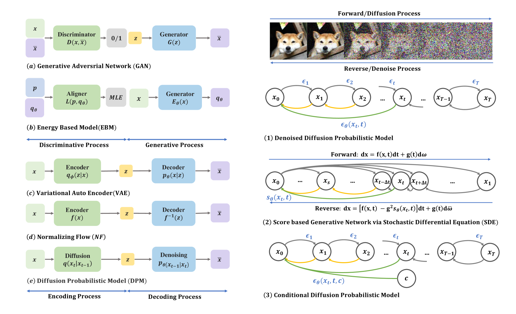
如何让机器拥有像人类一样的想象力？ 深度生成模型，包括变分自动编码器 (VAE) [1, 2]、基于能量的模型 (EBM) [3, 4]、生成对抗网络 (GAN) [5, 6]、归一化流 (NF) [7, 8] 和扩散模型 [9, 10, 11] 已证明在生成真实样本方面具有巨大的潜力。 在本次调查中，我们的重点在于扩散模型，它集中体现了该领域的前沿进展。 这些模型有效地克服了在 VAE 中对齐后验分布所带来的障碍，减轻了 GAN 对抗性目标固有的不稳定性，解决了 EBM 训练期间与马尔可夫链蒙特卡罗 (MCMC) 方法相关的计算负担，并强制执行类似于 NF 的网络约束。 因此，扩散模型在各个领域获得了广泛的关注，包括计算机视觉[12,13,14]、自然语言处理[15,16]、时间序列[17, 18]、音频处理[19, 20]、图形生成[21, 22]和生物信息学[23, 24 ]。 尽管扩散模型引起了人们的极大兴趣和关注，但仍然明显缺乏包含该领域研究进展的最新且全面的分类法和分析。

扩散模型包含两个相互关联的过程：一个预定义的前向过程，将数据分布映射到更简单的先验分布（通常是高斯分布），以及相应的反向过程，该过程采用经过训练的神经网络，通过模拟普通或随机分布来逐渐逆转前向过程的影响。随机微分方程 (ODE/SDE) [11, 25]。 前向过程类似于具有时变系数[25]的简单布朗运动。 神经网络经过训练，利用去噪得分匹配目标[26]来估计得分函数。 因此，与 GAN 中使用的对抗性目标相比，扩散模型提供了更稳定的训练目标，并且与 VAE、EBM 和 NF 相比表现出卓越的生成质量[27, 11]。

然而，必须承认，与 GAN 和 VAE 相比，扩散模型本质上需要更耗时的采样过程。 这源于通过利用 ODE/SDE（常微分方程/随机微分方程）或马尔可夫过程将先验分布迭代转换为复杂的数据分布，在逆过程中需要进行大量的函数评估。 此外，其他挑战包括逆过程的不稳定性、与高维欧几里德空间中的训练相关的计算需求和约束，以及似然优化中涉及的复杂性。 为了应对这些挑战，研究人员提出了多种解决方案。 例如，提出了先进的 ODE/SDE 求解器来加快采样过程[28, 29, 30]，同时采用了模型蒸馏策略[31, 14]以达到同样的目标。 此外，还引入了新颖的前向过程来增强采样稳定性[32,33,34]或促进降维[35,36]。 此外，最近的一系列研究致力于利用扩散模型来有效地桥接任意分布[37, 38]。 为了提供系统概述，我们将这些进步分为四个主要领域：采样加速、扩散过程设计、似然优化和桥接分布。 此外，这项调查将全面研究扩散模型在不同领域的多样化应用，包括计算机视觉、自然语言处理、医疗保健等。 它将探讨扩散模型如何成功应用于图像合成、视频生成、3D生成、医学分析<等任务/t3>、文本生成、语音合成、时间序列生成、分子设计和图形一代。 通过强调这些应用，我们的目标是展示扩散模型在现实场景中的实用性和变革潜力。

其余部分的结构如下：2 部分概述了扩散模型的基本公式和理论。 3部分探讨了该领域的算法改进，而4部分则介绍了基于生成机制的分类应用程序。 最后，在5节中，我们总结了内容，讨论了与其他扩散调查的联系，并确定了扩散模型的局限性和未来方向。

2 预赛

2.1 概念和定义

2.1.1 时间和状态

在扩散模型中，该过程在时间轴上展开，该时间轴可以是连续的也可以是离散的。 该时间线内的状态代表描述模型进展的数据分布。 噪声逐渐添加到初始分布中，表示为起始状态$x_0$，它是从数据分布$p_0$中采样的。 该分布逐渐向已知的噪声分布（通常是高斯分布）收敛，称为先前状态$x_T$。 起始状态和先前状态之间的状态是中间状态$x_t$，每个状态都与边际分布$p_t$相关联。 这使得扩散模型能够探索数据分布随时间的演变，并生成近似先前状态$x_T$的样本。 该进展通过一系列中间状态发生，每个状态映射到扩散过程中的特定时间点。

2.1.2 正向/反向过程和转换内核

在扩散模型中，前向过程$F$将起始状态转换为先验高斯噪声，而反向过程$R$使用转换核将先验状态去噪回到起始状态。 遵循DDPM[10]，通过定义扩散和去噪过程之间的转移核来推广扩散模型的离散公式。

$$F(x_0,\sigma )=F_T(x_{T-1},{\sigma }_T)\mathrm{\cdots }\circ F_t(x_{t-1},{\sigma }_t)\mathrm{\cdots }\circ F_1(x_0,{\sigma }_1)$$ (1)

$$R(x_T,\sigma )=R_1(x_1,{\sigma }_1)\mathrm{\cdots }\circ R_t(x_t,{\sigma }_t)\mathrm{\cdots }\circ R_T(x_T,{\sigma }_T)$$ (2)

其中 $F_t$ 和 $R_t$ 表示时间 $t$ 时的正向和反向转换内核，噪声尺度 ${\sigma }_t$ 来自噪声集 $\sigma$。 与归一化流模型不同，扩散模型包含可变噪声，逐渐细化分布以实现向目标分布的受控转变，从而提供更广泛的生成空间和可控生成。 离散框架提供了连续扩散过程的离散时间近似，允许实际实现和高效计算。

2.1.3 从离散到连续

当扰动核足够小时，离散过程（方程(1)和方程(2)）可以推广为连续过程。 [11] 表明，具有离散马尔可夫链 [9, 10] 的扩散模型可以合并到连续随机微分方程 (SDE) 框架中，其中生成过程反转固定前向扩散过程。 还导出了与逆 SDE 稍等价的储备 ODE[11]。 连续过程享有更好的理论支持，并为将 ODE/SDE 社区中的现有技术应用于扩散模型打开了大门。

2.2 背景

在本小节中，我们介绍三个基础公式去噪扩散概率模型、评分SDE公式和条件扩散概率模型，建立联系到第 3 部分和第 4 部分。 下面的数学公式可以看作2.1.2节中总体框架的具体形式。

图1： 扩散模型概述。 （左）生成模型简介。 GAN 和 EBM 首先利用生成器来捕获数据分布。 通过从训练数据中采样，根据真实分布来校正估计分布。 分布捕获过程以及区分标准有所不同。 VAE、NF和DPM通过编码过程直接将真实分布投影到预定义的分布中。 实例是通过对预定义分布的样本进行解码来获得的。 它们应用不同的预定义分布$𝐳$和编码解码过程。 （右） 扩散模型的简化公式。 一般程序如下右上图所示。 数据分布扩散为随机高斯噪声，并通过去噪反转。 (1) DDPM（第2.2.1节）沿着离散时间线实现逐步扩散和去噪过程。 (2)SDE（第2.2.2节）建立连续时间线，通过基于函数的随机微分方程（SDE）实现状态间转换。 (3)CDPM(第2.3节)在DPM的每个采样步骤中采用条件$c$来实现可控生成。

2.2.1去噪扩散概率模型（DDPM）

DDPM转发过程： 在 DDPM 框架中，选择马尔可夫转移核的噪声系数 ${\beta }_1,{\beta }_2,\mathrm{\dots },{\beta }_T$ 序列，遵循常数、线性或余弦计划等模式，从而提高样本质量。 根据[10]，前向步骤定义为：

$$F_t(x_{t-1},{\beta }_t):=q(x_t|x_{t-1}):=𝒩(x_t;\sqrt{1-{\beta }_t}{x}_{t-1},{\beta }_t\text{𝐈})$$ (3)

由$x_0$到$x_T$的前向转移核组成，即前向扩散过程，通过马尔可夫核$q(x_t|x_{t-1})$给数据添加高斯噪声：

$$F(x_0,{\{{\beta }_i\}}_{i=1}^T):=q\left(x_{1:T}\mid x_0\right):=\prod _{t=1}^{T}q\left(x_t\mid x_{t-1}\right)$$ (4)

DDPM逆向过程： 具有由 $\theta$ 参数化的可学习高斯核的逆过程定义为：

$$R_t(x_t,{\mathrm{\Sigma }}_{\theta }):=p_{\theta }(x_{t-1}|x_t):=𝒩(x_{t-1};{\mu }_{\theta }(x_t,t),{\mathrm{\Sigma }}_{\theta }(x_t,t))$$ (5)

${\mu }_{\theta }$和${\mathrm{\Sigma }}_{\theta }$是反向高斯核的可学习均值和方差，由反向步分布$p_{\theta }$确定。 从$x_T$到$x_0$的反向步骤的顺序是：

$$R(x_T,{\mathrm{\Sigma }}_{\theta }):=p_{\theta }\left(x_{0:T}\right):=p\left(x_T\right)\prod _{t=1}^T{p}_{\theta }\left(x_{t-1}\mid x_t\right)$$ (6)

DDPM旨在通过联合概率分布$p_{\theta }(x_0)=\int p_{\theta }(x_{0:T})𝑑x_{1:T}$来近似数据分布$p_0$。

扩散训练目标： 训练目标相当于通过引入 KL-Divergence $D_{\mathrm{KL}}$ 来最小化负对数似然的变分界限：

$𝔼\left[-\log p_{\theta }\left({\mathrm{x}}_0\right)\right]$ $\le {𝔼}_q[\underset{L_T}{\underbrace{D_{\mathrm{KL}}\left(q\left(x_T\mid x_0\right)\parallel p\left(x_T\right)\right)}}$ (7)

$+{\displaystyle \sum _{t>1}}\underset{L_{t-1}}{\underbrace{D_{\mathrm{KL}}(q(x_{t-1}\mid x_t,x_0)\parallel p_{\theta }(x_{t-1}\mid x_t))}}$

$\underset{L_0}{\underbrace{-\log p_{\theta }\left(x_0\mid x_1\right)}}]$

其中$L_T$和$L_0$表示先验损失和重建损失； $L_{1:T-1}$表示同时向前和向后步骤的后验之间的散度和。 简化$L_{t-1}$，我们根据后验$q(x_{t-1}|x_t,x_0)$获得名为$L_{simple}$的简化训练目标：

$$q\left(x_{t-1}\mid x_t,x_0\right)=𝒩(x_{t-1};{\widetilde{𝝁}}_t(x_t,x_0),{\tilde{\beta }}_{t}I)$$ (8)

其中 $\widetilde{{\beta }_t}$ 取决于 ${\beta }_t$。 保持上述参数化并将 $x_t$ 重新参数化为 $x_t(x_0,\sigma )$,$L_{t-1}$ 表示为 ${\mathrm{\ell }}_2$ 的期望 - 两个平均系数之间的损失：

$$L_{t-1}={𝔼}_q\left[\frac{1}{2{\sigma }_t^2}{\Vert {\widetilde{𝝁}}_t({\mathrm{x}}_t,{\mathrm{x}}_0)-{𝝁}_{\theta }({\mathrm{x}}_t,t)\Vert }^2\right]+C$$ (9)

这与下一段中讨论的去噪分数匹配相关。 通过重新参数化 ${\mu }_{\theta }$ w.r.t ${ϵ}_{\theta }$ 来简化 $L_{t-1}$，简化的训练目标名为 $L_{simple}$：

$$L_{simple}:={𝔼}_{x_0,ϵ}\left[\frac{\beta _t^{}{}_{}{}^2}{2\sigma _T^{}{}_{}{}^2{\alpha }_t(1-{\overline{\alpha }}_t)}\right]{\Vert ϵ-{\mathit{ϵ}}_{\theta }(\sqrt{{\overline{\alpha }}_t}{x}_0+\sqrt{1-{\overline{\alpha }}_t}ϵ)\Vert }^2$$ (10)

大多数扩散模型使用 DDPM 训练策略。 然而，改进的DDPM建议将$Lsimple$与其他目标结合起来。 训练后，预测网络${\mathit{ϵ}}_{\theta }$用于逆向过程中进行祖先采样。

2.2.2 对SDE公式进行评分

Score SDE [11]将DDPM中的离散时间方案扩展到基于随机微分方程的连续时间框架。 此外，它还提出了基于 ODE 公式的附加确定性采样框架。

转发SDE： ScoreSDE [11]连接了连续扩散过程和随机微分方程。 相反的过程与 Itô SDE [39] 的解相关，由均值漂移的漂移项和附加噪声的布朗运动组成：

$$dx=f(x,t)dt+g(t)dw,t\in [0,T]$$ (11)

其中 $w_t$ 是标准的维纳过程，$f(\cdot ,t)$ 是 $x(t)$ 的漂移系数，$g(\cdot )$ 是与 $x$ 无关的简化扩散系数。$p_t(x)$ 和 $p_T$ 分别表示边际分布和先验分布。 如果系数是分段连续的，则正向 SDE 方程有唯一解[40]。 提出了两种类型的前向过程：变异保持（VP）和变异爆炸（VE）SDE。 VP对应DDPM框架的不断扩展：

VP: $\mathrm{d}x=-{\displaystyle \frac{1}{2}}\beta (t)xdt+\sqrt{\beta (t)}\mathrm{d}w$

VE: $\mathrm{d}x=\sqrt{{\displaystyle \frac{\mathrm{d}\left[{\sigma }^2(t)\right]}{\mathrm{d}t}}}\mathrm{d}w$

逆向 SDE： 扩散模型的采样是通过前向过程的相应逆时 SDE 完成的（方程 (11)）[41]：

$$\mathrm{d}x=\left[f(x,t)-g{(t)}^2{\nabla }_x\log p_t(x)\right]\mathrm{d}\overline{t}+g(t)\mathrm{d}\overline{w},t\in [0,T]$$ (12)

其中$w_t$是标准维纳过程，$f(\cdot ,t)$是$x(t)$的漂移系数，$g(\cdot )$是简化的扩散系数。 $p_t(x)$ 和 $p_T$ 是边际分布和先验分布。 如果系数是分段连续的，则正向 SDE 方程存在唯一解。 [42]：

$L:={𝔼}_t$ $\{\lambda (t){𝔼}_{x_0}{𝔼}_{q(x_t|x_0)}[\parallel s_{𝜽}(x_{t}t)-{\nabla }_{x_t}\log p(x_t|x_0){\parallel }_2^2]\}$ (13)

其中 $x_0$ 是从分布 $p_0$ 中采样的，$\lambda (t)$ 是正权重函数，用于将时间相关损失保持在相同的量级 [11]. $q(x_t|x_0)$ 是与式（1）中的前向过程相关的高斯转移核。 (11)。 例如，$q(x_t|x_0)=𝒩(x_t;x_0,{\sigma }^2(t)\text{𝐈})$。 可以证明，对于几乎所有 $x,t$，去噪得分匹配目标（方程 (13)）中的最优解等于真实得分函数 ${\nabla }_x\log p_t(x)$ 。 此外，评分函数$s_{\theta }$可以看作是DDPM目标中神经预测${\mathit{ϵ}}_{\theta }$的重新参数化（方程(10)）。 [43]进一步表明，扩散模型前向过程中的得分函数可以分解为三个阶段。 当从近场移动到远场时，扰动数据会受到数据分布中更多模式的影响。

概率流常微分方程： 概率流 ODE [11] 支持与 SDE 具有相同边际概率密度的确定性过程。 受 Maoutsa et al. [44] 和 Chen et al. [45] 的启发，任何类型的扩散过程可以导出为一种特殊形式的 ODE。 方程相应的概率流 ODE。 (12) 是

$$dx=\{f(x,t)-\frac{1}{2}g{(t)}^2{\nabla }_x\log p_t(x)\}dt$$ (14)

与 SDE 相比，概率流 ODE 可以用更大的步长求解，因为它们不具有随机性。 因此，PNDMs[46]和DPM-Solver[47]等一些工作基于先进的ODE求解器获得了更快的采样速度。

2.3 条件扩散概率模型

扩散模型是通用的，能够从无条件 $p_0$ 和条件 $p_0(x|c)$ 分布生成数据样本，以 $c$ 作为给定条件，例如类标签或文本链接到数据$x$[36]。 评分网络$s_{\theta }(x,t,c)$在训练期间整合了这个条件。 各种采样算法，包括无分类器指导[48]和分类器指导[27]，都是为条件生成而设计的。

标记条件 使用标记条件采样指导每个采样步骤的梯度。 它通常需要具有 UNet 编码器架构的附加分类器来生成特定标签的条件梯度，这些标签可以是文本、分类、二进制或提取的特征 [27, 49, 28, 50, 51, 52, 53, 54 , 55, 12]。 该方法首先由[27]提出，支撑了当前的条件采样技术。

无标签条件 无标签条件采样使用自我信息作为指导，通常以自我监督的方式应用[56, 57]。 它通常用于去噪[58]、绘制图像[59]和修复任务[17]。

表一： 扩散算法改进的分类（第 3 节）

for tree= grow=east, reversed=true,anchor=base west, parent anchor=east, child anchor=west, base=left, rectangle, draw=black, rounded corners,align=left, minimum width=3em, edge+=darkgray, line width=1pt, inner xsep=4pt, inner ysep=1pt, , where level=1text width=5em,fill=orange!10, where level=2text width=5em,fill=blue!10, where level=3yshift=0.26pt,fill=pink!30, where level=4yshift=0.26pt,fill=yellow!20, where level=5yshift=0.26pt, [Diffusion
Algorithm
Improvement, text width=8em, fill=green!20, [Sampling
Acceleration, text width=7em [Knowledge
Distillation, text width=5em, [ODE Trajectory, text width=6.6em [Progressive Distill [31]/TRACT [60]
Denoising Student [61]/DSNO [62]
Consistency Model [14]/RCFD [63]
Recfied Flow [64]/SFT-PG [65]
MMD-DDM [66]/ [67, 68] ] ] [SDE Trajectory, text width=6.6em [Recfied Flow [37]/I2SB [69]
Stochastic interpolant [38]/DDIB [70] ] ] ] [Training
Scheme ,text width=4.5em [Diffusion Scheme
Learning ,text width=8em [TDPM[71]/Blurring Diffusion[72]
ES-DDPM[73]/Soft Diffusion[74]
CCDF[58]/[75, 76] ] ] [Noise Scale Design, text width=8.4em [VDM [77]/Improved DDPM [78]
FastDPM [79]/[80] ] ] ] [Training-Free
Sampling ,text width=6.6em [ODE, text width=3em [DDIM [26]/gDDIM [81]/EDM [25]
DEIS [29]/PNDM [46]/DPM-Solver [47] ] ] [SDE, text width=3em [Gotta Go Fast [29] EDM [25]/Restart [30] ] ] [Analytical, text width=4.4em [Analytic-DPM [82]/SN&PNR-DDPM [83] ] ] [Dynamic
Programming, text width=6em [DDSS [84]/Efficient Sampling[85] ] ] ] [Model
Merging, text width=4.5em [GAN-based, text width=5em [TDPM [71]/Denoising GAN [86] ] ] [VAE-based, text width=5em [DiffuseVAE[87]/ES-DDPM[73] ] ] ] ] [Diffusion
Process Design, text width=7em [Latent Space, text width=6em [LSGM [35]/INDM [88]/Latent Diffusion [36]/DVDP [89] ] ] [Innovative
Forward
Processes, text width=6em [PFGM [32]/PFGM++ [33]/Cold Diffusion[90]
Flow-Matching [91]/EDM [25]/CLD [34] ] ] [Non-Euclidean, text width=6.5em [Discrete, text width=4em, [D3PM [16]/Argmax [92]/ARDM [93]
VQ-diffusion[94]/VQ-Diffusion+[95]/[96] ] ] [Manifold, text width=5em [RGSM [97]/PNDM [46]/RDM [98]
Boomerang [99]/[100] ] ] [Graphs, text width=5em [EDP-GNN [22]/Graph GDP [21]
NVDiff [101]/[102] ] ] ] ] [Likelihood
Optimization, text width=7em [MLE Training, text width=7.5em [ScoreFlow [103]/VDM [77]/[104] ] ] [Hybrid Loss, text width=7.5em [improved-DDPM [49]/[105] ] ] ] [Bridging
Distributions, text width=7em [$\alpha$-blending [106]/Recfied Flow [37]/I2SB [69]
Stochastic interpolant [38]/DDIB [70], text width=22em ] ] ]

3 算法改进

尽管跨不同数据模式生成了高质量的扩散模型，但它们的实际应用仍有待改进。 与 GAN 和 VAE 等其他生成模型不同，它们需要缓慢的迭代采样过程，并且它们的前向过程在高维像素空间中运行。 本节重点介绍增强扩散模型的四个最新进展：(1) 采样加速技术（第3.1节），以加速标准 ODE/SDE 模拟； (2) 新的前向过程（第 3.2 节），用于改进像素空间中的布朗运动； (3) 似然优化技术（第3.3节），用于增强扩散 ODE 似然； (4) 桥接分布技术（第3.4

3.1 采样加速

尽管具有高保真度，但扩散模型的实际用途因其采样速度慢而受到限制。 本节简要概述了提高采样速度的四种先进技术：蒸馏、训练计划优化、免训练加速以及扩散模型与更快的生成模型的集成。

3.1.1 知识蒸馏

知识蒸馏是一种将“知识”从较大模型转移到更简单模型的技术，正变得越来越流行[107, 108]。 在扩散模型中，目标是通过对齐和最小化原始样本和生成样本之间的差异，使用更少的步骤或更小的网络来生成样本。 作为跨分布的轨迹优化，蒸馏提供了最佳映射，以实现经济高效且更快的可控发电。

ODE 轨迹 使用 ODE 公式从教师模型到学生模型的知识蒸馏，通过分布领域的有效路径将先验分布映射到目标分布。 [31]首先应用这一原理通过逐步提炼采样轨迹、每两步拉直潜在映射来改进扩散模型。 TRACT [60]、Denoising Student [61] 和一致性模型 [14] 扩展了这种效果，将加速度提高到 64 和 1024，通过直接从时间 $T$ 的噪声样本中估计干净数据。 RFCD [63] 通过在训练期间对齐样本特征来增强学生模型的性能。

通过最优传输[109]可以获得最优轨迹。 通过流匹配最小化分布之间的传输成本，ReFlow [64]和[67]实现了一步生成。 DSNO [62]提出了一种用于直接时间路径建模的神经算子。 一致性模型[14]、SFT-PG [65]和MMD-DDM [66]使用LPIPS、IPA和分别是MMD。

SDE 轨迹 提取随机轨迹仍然具有挑战性。 提出的工作很少（参见3.4节）。

3.1.2培训日程

改进训练计划涉及修改与采样无关的传统训练设置，例如扩散方案和噪声方案。 最近的研究强调了训练方案中影响学习模式和模型性能的关键因素。 在本小节中，我们将训练增强分为两个主要领域：扩散方案学习和噪声尺度设计。

扩散方案学习扩散模型将数据投影到像变分自动编码器（VAE）这样的潜在空间中，由于其更高的表达能力而更加复杂。 这些模型中的逆解码方法可以分为两种方法：编码度优化和投影方法。

编码度优化方法，例如 CCDF [58] 和 Franzese 等人 [75]，通过将扩散步骤数视为多变的。 截断是另一种方法，它通过以一步方式从分散程度较低的数据中进行采样来平衡生成速度和样本保真度。 TDPM [71] 和 ES DDPM [73] 使用 GAN 和 CT [110] 进行截断。 投影方法，如软扩散[74]和模糊扩散模型[72]，使用模糊和掩模等线性损坏来探索扩散核的多样性。

噪声尺度设计 在传统的扩散过程中，每个过渡步骤都是由注入的噪声决定的，相当于在正向和反向轨迹上随机游走。 设计噪声尺度可以导致合理的生成和快速收敛。 与传统的 DDPM 不同，现有方法将噪声尺度视为整个过程中可学习的参数。

VDM [77] 等前向噪声设计方法将噪声尺度参数化为信噪比，并将其与训练损失和模型类型联系起来。 FastDPM [79] 使用离散时间变量或方差标量将噪声设计与 ELBO 优化联系起来。 对于反向噪声设计，改进的 DDPM [78] 通过训练混合损失来隐式学习反向噪声尺度，而 San Roman et al. 使用噪声预测网络来更新在祖先采样之前反转噪声尺度。

3.1.3 免训练采样

免训练方法旨在利用先进的采样器来加速预训练扩散模型的采样过程，从而消除模型重新训练的需要。 本小节将这些方法分为几个方面：扩散 ODE 和 SDE 采样器的加速、分析方法和动态规划。

ODE 加速 [11] 证明 DDPM 中的随机采样过程具有边际等效概率 ODE，它定义了数据分布之前的确定性采样轨迹。 鉴于 ODE 采样器产生的离散化误差比随机采样器 [11, 30] 更小，因此之前大多数有关采样加速的工作都是以 ODE 为中心的。 例如，广泛使用的采样器DDIM [26]可以被视为概率流ODE [11]：

$$\mathrm{d}\overline{x}(t)={ϵ}_{\theta }^{(t)}\left(\frac{\overline{x}(t)}{\sqrt{{\sigma }^2+1}}\right)\mathrm{d}\sigma (t)$$ (15)

其中${\sigma }_t$由$\sqrt{1-{\alpha }_t}/\sqrt{{\alpha }_t}$参数化，$\overline{x}$由$x/\sqrt{{\alpha }_t}$参数化。 后来的作品[29, 47]将DDIM解释为在保方差（VP）扩散[11]的ODE上应用指数积分器的产物。 先进的 ODE 求解器已用于 PNDM [46]、EDM [25]、DEIS [29]、gDDIM 等方法[81] 和 DPM 求解器[47]。 例如，EDM 采用 Heun 的 $2^{\text{nd}}$ 阶 ODE 求解器，DEIS/DPM 求解器通过在每个离散时间间隔内对分数函数进行数值近似来改进 DDIM。 与原始 DDPM 采样器相比，这些方法显着加快了采样速度（减少了函数评估或 NFE 的数量），同时仍然产生高质量的样本。

SDE 加速 基于 ODE 的采样器速度更快，但达到性能限制，而基于 SDE 的采样器尽管速度较慢，但​​提供更好的样本质量。 有几项工作专注于加快随机采样器的速度。 Gotta Go Fast [111] 使用自适应步长来实现更快的 SDE 采样，而 EDM [25] 将高阶 ODE 与类似 Langevin 动力学的噪声添加和去除相结合，证明他们提出的随机采样器在 ImageNet-64 上明显优于 ODE 采样器。 最近的一项工作[30]表明，尽管 ODE 采样器涉及较小的离散化误差，但 SDE 中的随机性有助于缩小累积误差。 这导致了重新启动采样算法[30]，它融合了两个领域的最佳方面。 该采样方法交替通过额外的前向步骤添加显着噪声和严格遵循后向 ODE，在标准基准和稳定扩散模型[36]上超越了以前的 SDE 和 ODE 采样器，无论是在速度还是在准确性。

分析方法 现有的免训练采样方法将逆协方差尺度视为手工制作的噪声序列，而不动态考虑它们。 从KL散度优化开始，分析方法使用蒙特卡罗方法设置反向均值和协方差。 Analytic-DPM [82] 和扩展 Analytic-DPM [83] 联合提出每个状态校正下的最优逆解。 解析方法对近似误差有理论上的保证，但由于其预先假设，它们仅限于特定的分布。

动态规划调整 动态规划（DP）通过记忆技术[112]实现对所有选择的遍历，在更短的时间内找到最优解。 假设从一种状态到另一种状态的每条路径与其他状态共享相同的 KL 散度，动态规划算法会探索沿轨迹的最佳遍历。 当前基于DP的方法[85, 113]通过优化ELBO损失的总和来降低$𝒪\left(T^2\right)$计算成本。

3.1.4 合并扩散和其他生成模型

扩散模型可以与其他生成模型（例如生成对抗网络（GAN）或变分自动编码器（VAE））协同作用，以简化采样过程。 例如，原始数据$x_0$可以通过在中间阶段从噪声样本获得的VAE[87]或GAN[86]直接预测扩散采样过程。 此外，VAE [73] 或 GAN [71] 可以在中间扩散时间步生成样本，然后通过扩散模型对其进行去噪，直到时间 $t=0$ 更快的时间穿越。

3.2 扩散工艺设计

扩散模型中的传统前向过程通常被视为像素空间中的布朗运动[10, 25]，对于生成建模来说可能不是最佳的。 因此，研究工作致力于创建新的扩散过程，以简化和增强神经网络的相关后向过程。 这条路径分为开发为扩散模型设计的潜在空间（第3.2.1节）和用像素空间中的改进版本取代传统的前向过程（第3.2.2节） 。 还特别关注专门为非欧几里得空间（如流形、离散空间、函数空间和图）定制的扩散过程（第 3.2.3 节）。

3.2.1 潜在空间

研究人员在学习的潜在空间中探索训练扩散模型，以增强神经网络并建立更直接的后向过程。 这种方法以 LSGM [35] 和 INDM [114] 为例，它们联合训练扩散模型和 VAE 或归一化流模型。 两个模型都有一个共同的目标，即加权去噪得分匹配损失（方程(13)中的$L_{DSM}$)，以优化编码器-解码器和扩散模型对。

$$L:=L_{Enc}(z_0|x)+L_{Dec}(x|z_0)+L_{DSM}\left(\left({\left\{z_t\right\}}_{t=0}^T\right)\right)$$ (16)

这里，$z_0$表示原始数据$x$的潜在形式，而$z_t$是其扰动的对应物。 值得注意的是，$z_t$是编码器的函数，因此$L_{DSM}$损失也会更新编码器的参数。 联合目标是优化 ELBO 或对数似然 [35, 114]。 这导致了一个更容易学习和采样的潜在空间。 Stable Diffusion [36] 等有影响力的工作将过程分为两个阶段：学习 VAE 的潜在空间和以文本作为条件输入训练扩散模型。 另一方面，DVDP [89] 将像素空间分解为正交分量，并在图像扰动期间动态调整每个分量的衰减，类似于动态图像下采样和上采样。

3.2.2 新兴的前沿进程

潜在空间扩散具有优点，但也增加了框架的复杂性和计算负担。 为了解决这个问题，当代研究探索了正向过程设计，以获得更稳健和更复杂的生成模型。 例如，泊松场生成模型 (PFGM)[32] 将数据视为增广空间中的电荷，引导沿电场线的简单分布朝向数据分布。 该模型中的前向过程是在电场线方向上定义的，表现出比扩散模型更稳健的后向采样。 PFGM++ [33] 使用更高维度的增强变量扩展了 PFGM，这些模型之间的插值揭示了最佳点，从而生成最先进的图像。 PFGM 和 PFGM++ 还在抗体 [115] 和医学图像 [116] 生成中得到应用。

Dockhorn 等人[34]引入了临界阻尼朗之万扩散（CLD）模型，该模型结合了通过哈密顿动力学相互作用的“速度”变量。 与直接学习数据的得分函数相比，该模型简化了条件速度分布得分函数的学习。 鉴于扩散模型和 PFGM 等受物理启发的生成模型的成功，最近的一项工作[117]提供了一种将物理过程转化为生成模型的系统方法。

其他研究探索替代的腐败过程。 例如，冷扩散[90]使用任意图像变换（例如前向过程中的模糊），而[118]在像素空间中应用散热。 此外，还努力使用高级高斯扰动内核[25, 91]来增强训练和采样。

3.2.3 非欧空间上的扩散模型

离散空间深度生成模型在自然语言处理[119, 120]、多模态学习[49, 121]等各个领域取得了长足的进步，以及科学人工智能[122, 123]。 一项关键成就是离散数据的处理，包括句子、残差、原子和矢量量化数据。 扩散模型通常用于这些应用程序，重点关注文本、分类数据和矢量量化数据。 D3PM [16] 定义了离散空间中的前向过程，使用转换内核 $Q_t$ 处理文本或原子类型等数据：

$$q\left(x_t\mid x_{t-1}\right)=\mathrm{Cat}(x_t;p=x_{t-1}{𝑸}_t)$$ (17)

其中 $\mathrm{Cat}()$ 表示分类分布。 这种方法已扩展到生成语言文本、分段图和无损压缩[92, 93]。

对于文本到图像生成和文本到 3d 生成等多模态问题，矢量量化（VQ）数据将数据转换为代码，在自回归编码器中实现了优异的性能[124]。 [94]首先将扩散技术应用于VQ数据，解决了VQ-VAE中的单向偏差和累积预测误差。 这一核心思想已在进一步的文本到图像、文本到姿势和文本到多模态工作[125,95,126,127,128,129]中得到利用。 前向过程由概率转移矩阵$Q$和分类表示向量$v$定义：

$$q\left(x_t\mid x_{t-1}\right)={𝒗}^{\top }\left(x_t\right){𝑸}_t𝒗\left(x_{t-1}\right)$$ (18)

流形 图像和视频等数据结构通常位于欧几里得空间中。 然而，机器人学 [130]、地球科学 [131] 和蛋白质建模 [132] 等领域的某些数据是在黎曼流形内定义的[133]。 标准欧几里得方法可能不适用于此环境。 为了解决这个问题，最近的方法，如 RDM [98]、RGSM [97] 和 Boomerang [99] 已将扩散采样纳入到黎曼流形，扩展分数SDE框架[11]。 理论著作[100, 46]为流形采样提供了进一步的支持。

图 基于图的神经网络因其在人体姿势 [127]、分子 [134] 和蛋白质 [135] [136]。 当前的方法将扩散理论应用于图。 EDP​​-GNN [22]、Pan 等人 [102]和 GraphGDP [21] 等方法通过邻接矩阵处理图数据以捕获排列不变性。 NVDiff [101] 使用反向 SDE 重建节点位置。

函数 Dutordoir 等人、[137]引入了第一个在函数空间中采样的扩散模型，通过联合后验采样捕获无限维分布。

3.3 似然优化

虽然扩散模型[10]优化了ELBO以克服对数似然的棘手问题，但似然优化被忽略，这对于连续时间扩散模型[11]来说是一个挑战>。 包括 MLE 训练（第 3.3.1 节）和混合损失（第 3.3.2 节）在内的两种方法旨在增强训练的可能性。

3.3.1 MLE训练

三个并行工作——ScoreFlow [103]、VDM [77] 和 [104] 在 MLE 训练和加权去噪之间建立联系扩散模型中的分数匹配（DSM）目标，主要通过使用吉尔萨诺夫定理。 例如，ScoreFlow [103] 表明，在特定的加权方案下，DSM 目标提供了负对数似然的上限。 这一发现使得基于分数的 MLE 能够实现与神经网络参数无关的近似。

3.3.2 混合损失

某些方法不是仅仅依赖最大似然训练，而是引入混合损失设计来提高 DSM 中的模型似然。 其中一种方法是改进的 DDPM [78]，它提出使用简单的重新参数化技术和结合变分下界和 DSM 的混合学习目标来学习逆过程的方差。 此外，[105] 表明，合并高阶分数匹配损失有助于增强对数似然。

3.4 桥接分布

扩散模型擅长转换简单的高斯分布，但在桥接任意分布时面临挑战，特别是在图像到图像转换和细胞分布传输等领域。 已经提出了各种方法来解决这个问题。 一种方法称为$\alpha$-混合[106]，涉及迭代混合和去混合以创建确定性桥。 当一端分布为高斯分布时，扩散模型被视为特殊情况。 另一种方法是整流流[37]，它包含额外的步骤来拉直桥梁。 其他方法（例如 [38] 中提出的方法）建议使用两个分布之间的通用插值函数构造 ODE。 此外，其他人探索利用薛定谔桥[69]或高斯分布作为连接点来连接两个扩散ODE[70]。

表二： 基于扩散的模型应用分类（第4节）

对于树=生长=东，反向=真，锚点=基西，父锚点=东，子锚点=西，基=左，矩形，绘制=黑色，圆角，对齐=左，最小宽度= 2.5em，内部xsep=4pt，内部 ysep=1pt，，其中 level=1text width=5em，fill=blue！6，其中 level=2text width=5em，fill=pink！30，其中 level=3yshift=0.26pt，fill=yellow！ 20，其中 level=4yshift=0.26pt，其中 level=5yshift=0.26pt，[扩散

应用，fill=orange!10，[图片

生成，文本宽度=5em [无条件和

类条件，文本宽度=7.5em [DDPM[10]/ Imagen [138]/diffuisonbeats gan [27] ] ] [Text

条件，文字宽度=5em [Imagen[138]1>/稳定扩散 [36]2>/DALL-E 2 [121]3>/ [139, 140, 141]4> ] ] [图像

条件，文字宽度=5em [Instructpix2pix[142]6>/[143]7> ] ] ] [3D8>

生成0>，文本宽度=5em [3D条件，文本宽度=6em [PDR[144]1>/Shape-E [145]2>/Point-E [146]3>/PVD[147]4>

0-1-3 [148]6>/One-2-3-45 [149]7>/[150, 151]8>] ] [二维条件，文本宽度=6em [DreamFusion[152]9>/Magic3d[ 153]0>] ] ] [视频1>

世代3>，文字宽度=5em [世代，文字宽度=5em [VDM[12] 4>/制作视频[154]5>/MCVD[155]6>/FDM[156]7>

RVD[157]9>/RaMViD[158]0>/AnimatedDiff [159]1> ] ] [医疗2>

分析4>，文本宽度=5em [分布中，文本宽度=6em [MCG [160]5>/Score-MRI [161]6>/Diff- MIC [162]7>

OCT-DDPM [163]9>/CCDF[58]0>] ] [跨-

分布，文本宽度=6em [AnoDDPM [164]2>/FNDM [165]3>/DifuseMorph [166]4>

R2D2+ [ 167]6>/3D-DDPM-Med [168]7>/ [169, 170]8> ] ] ] [文字9>
生成1>，文本宽度=5em [离散[D3PM[16]2>/Argmax[92]3>/DiffusionBERT[171]4> ] ] [潜在[扩散-LM[15]5>/Seqdiffuseq [172]6>/GENIE [173]7>/LIVE[ 174]8>

DiffuSeq [175]0>/AR-Diffusion [176]1>/Difformer [177]2>/SED [178]3>/ [179]4> ] ] ] [时间序列5>

世代7>，文字宽度=5.4 em [插补，文本宽度=5em [TSGM [180]8>/CSDI[17]9>/PriSTI [181]0>/SSSD [ 182]1>/TransFusion[183]​​2> ] ] [预测，文本宽度=5em [TimeGrad[184]3>/ScoreGrad [18]4>/DiffSTG [185]5> ] ] ] [音频6> &

语音8>

生成0> ，文字宽度=5em [转换&

分离，文字宽度=6em [WaveGrad[19]2>/DiffWave[186]3>/DiffSinger[187] 4>

ProDiff[188]6>/BinauralGrad[189]7>/DiffSVC[190]8>/[191] 9> ] ] [内容

条件，文本宽度=6em [EdiTTS[192]1>/Diff-TTS[193]2>/SpecGrad[ 194]3>/ [195]4>

引导式 TTS[196]6>/DiffSound [197]7>/DiffSinger [187]8> ] ] ] [分子9>

世代
1>，文本宽度=5em [无条件，文本宽度=6.4em [GeoDiff [23]2>/EDM[198]3>/ProteinSGM[199]4>

扭转[200]6>/SE3Diffusion [201]7>/FoldingDIff [202]8>

] ] [多模态，文本宽度=6.4em [DiffDock [203]0>/DiffAb [24]1>/协同设计[135]2>

RFDiffusion [204]4>/ProteinGenerator [205]5> ] ] ] [图表6>

生成8>，文本宽度=5em [无条件，文本宽度=6.4em [GraphGDP [21]9> /DiGress [206]0>/EDP-GNN [22]1>] ] [有条件，文本宽度=6.4em [PCFI [207]2>/EDGE [208]3>/DiffFormer [209]4>/D4Explainer [210]5> ] ] ]

4 申请

受益于生成真实样本的强大能力，扩散模型已广泛应用于各个领域。 在实际应用中，发挥扩散模型威力的关键在于使扩散过程、去噪过程和条件采样适应各种数据的本质。 受这个想法的启发，扩散的应用概括为图像生成、3D生成、视频生成、医学分析、文本生成、时间序列生成、音频生成、分子设计和图形生成.

4.1 图像生成

扩散模型在图像生成方面取得了显着的性能，无论是在传统的类条件或无条件生成[27,10,138]上，还是在更复杂的文本或图像条件[36, 143]上，或其组合[142]。 今后我们的讨论将集中于模仿现实场景的应用程序设置，根据条件输入对应用程序进行分类。

4.1.1 文本条件

扩散模型在文本到图像生成方面表现出卓越的性能，不仅能够创建逼真的图像，而且能够创建紧密遵循用户提供的文本输入的样本。 著名的例子包括 Imagen [138]、Stable Diffusion [36] 和 DALL-E 2 [121]。 这些方法建立在现有的扩散架构之上，添加了交叉注意层，将文本嵌入序列注入扩散模型中。 实验结果表明，这种调节机制有效地将文本信息融合到生成的图像中。

此外，交叉注意条件机制通过利用和操作交叉注意层中的键、值或注意矩阵，可以实现许多免训练的图像编辑。 例如，[139]通过交换或添加新的特征图到交叉注意层的输出来改变源图像中的概念； [140] 通过学习新的文本嵌入作为交叉注意层的输入，可以定制新概念。 [141] 强制交叉注意力来关注文本提示中的所有主题标记并扩大它们的激活，从而鼓励模型忠实地生成文本提示中描述的所有主题。

4.1.2 图像条件

除了文本条件之外，扩散模型还支持图像条件作为条件输入，例如要编辑的图像、深度图或人体骨骼。 基本概念保持不变，涉及将编码图像特征合并到扩散主干中。 [142] 的工作将源图像中的编码特征引入到第一个卷积层中以实现图像调节，从而允许使用文本提示进行图像到图像的编辑。 类似地，[143]利用深度图、Canny边缘或人体骨骼来控制生成图像的空间布局。

4.2 3D生成

一般来说，通过扩散模型生成 3D 的主要方法有两种。 第一种方法侧重于直接使用 3D 数据训练这些模型。 然而，由于 3D 数据的可用性有限，第二种方法强调通过 2D 扩散先验生成 3D 内容。

4.2.1 3D数据条件

鉴于 3D 表示的多样性，例如 NeRF、点云、体素、高斯分布等，扩散模型已有效地应用于这些不同的 3D 表示。 例如，[151, 147, 150]等作品直接生成3D物体的点云。 为了实现高效采样，PDR[144]采用混合点体素表示进行形状处理，引入了点云补全的新范式。 在此研究的基础上，Point-E [146] 进一步将图像合成作为点云扩散模型的附加条件输入。

相比之下，Shape-E [145] 利用扩散模型来表示 3D 对象的 NeRF。 Zero-1-to-3 [148] 采用不同的方法，通过训练视点条件扩散模型来实现新颖的视图合成。 然后，它根据从不同相机视点生成的样本来优化 NeRF。 基于这项工作，[149]通过合并姿态估计阶段进一步扩展了 Zero-1-to-3。

4.2.2 二维扩散先验

另一个有趣的作品系列旨在 从 2D 扩散模型中提取 3D 模型。 Dreamfusion [152] 巧妙地使用分数蒸馏采样 (SDS) 目标从预先训练的文本到图像模型中提取 NeRF。 他们通过梯度下降优化随机初始化的 NeRF，从而使不同角度的渲染图像实现低损失。 [153]将DreamFusion扩展为两阶段从粗到细的优化框架，以加速生成过程。

4.3 视频生成

视频扩散模型通过附加时间轴增强了用于图像生成的 2D 扩散模型。 总体思路是添加一个时间层来显式建模现有 2D 扩散结构中的跨帧依赖性。 代表作品包括Video Diffusion Models [12]、Make-A-Video [154]、AnimatedDiff [159]、RVD [ 157]、FDM [156]、MCVD [155]。 RaMViD [158] 使用 3D 卷积神经网络将图像扩散模型扩展到视频，并设计了用于视频预测、填充和上采样的调节技术。

4.4 医学分析

扩散模型为医学分析中遇到的挑战提供了解决方案，在医学分析中获取大规模、高质量的带注释数据集具有挑战性。 这些模型在与分布内分析和跨分布生成相关的任务中表现出了卓越的性能。

4.4.1 分布内分析

扩散模型在各种医学成像任务中都很有效，利用其准确捕获具有强大先验信息的医学图像的能力。 它们已成功应用于超分辨率[160, 58]、分类[162]和噪声鲁棒性[161, 163]。 例如，Score-MRI [161] 使用像素引导 SDE 采样加速 MRI 重建，而 Diff-MIC [162] 通过双粒度引导实现跨多种模态的准确分类和最大均值差异。 此外，MCG[160]提出了CT超分辨率采样期间的流形校正，减少了误差并提高了加速度。

4.4.2 跨发行版生成

多模式指导显着提高了医学分析的生成能力。 通过集成特定类别的指导[165, 164]和像素级指导[166,165,169]，无条件去噪网络可以跨不同类型的稀缺图像执行图像转换图像，包括高质量格式图像、健康图像和无偏差图像。 著名的例子包括 FNDM [165]，它能够通过具有混合条件指导的非马尔可夫框架准确检测大脑异常，以及 DiffuseMorph [166]，它执行 MR使用以移动和固定图像对为条件的连续扩散采样进行图像配准。 此外，还有一些有前途的方法可以利用少量高质量样本[170,167,168]生成的真实医学图像来丰富训练数据集。 例如，在 31,740 个样本上训练的潜在扩散模型已用于合成具有 100,000 个实例的高质量且语义丰富的数据集，取得了令人印象深刻的 0.0076 [170] FID 分数。

4.5 文本生成

文本生成通过生成自然且连贯的语言，在缩小人类与先进人工智能之间的差距方面发挥着至关重要的作用。 自回归语言模型按顺序生成文本，确保高语义一致性，但生成速度较慢[211]。 另一方面，扩散模型可以实现并行文本生成，速度更快，但语义一致性相对较弱[212, 213]。 两种主要方法，即离散生成和潜在生成，通常用于解决生成离散 Token 的挑战。

4.5.1 离散生成

离散生成方法涉及以离散词作为输入的模型，并利用先进的技术、参数化和预训练模型。 D3PM [16] 和 Argmax [92] 等典型作品开创了扩散模型和离散生成之间的联系，将单词视为分类向量。 他们使用离散转移矩阵建立前向和后向过程，并将生成的数据视为平稳分布。 DiffusionBERT [171] 将扩散模型与预训练的语言模型相结合，展示了改进的文本生成性能。 此外，它还引入了一种新颖的噪声调度，并探索了将时间步合并到 BERT 中以实现反向扩散过程。

4.5.2 潜在一代

第二种方法侧重于在标记的潜在空间中生成文本，捕捉扩散过程的连续性。 它融合了增强的损失函数[172, 176, 177]、多样化的生成类型[175, 178]和先进的模型架构[15, 173] t2>。 例如，LM-Diffusion [15] 引入了基于 Transformer 的图形模型用于可控生成，在各种文本生成任务中展示了卓越的性能。 GENIE [173] 提出了一种基于扩散框架的大规模语言模型，结合了一种新颖的连续段落去噪（CPD）损失，以改进去噪和段落级连贯性。 它展示了基于扩散的解码器在文本生成方面的潜力，并为未来的研究提供了坚实的基础。 除了先进的条件采样、标记级捕获和后细化之外，NLP 中的扩散模型有望增强嵌入空间 [178, 213] 的建模，与大型预训练数据建立连接语言模型，并支持跨模态生成[174,179,212]。

4.6 时间序列生成

准确的时间序列建模对于趋势预测、决策和实时分析至关重要。 扩散模型通过时间序列数据模块增强了这一过程，从而实现卓越的分析和多样化的生成[214]。 根据不同类型的掩蔽策略，先验条件可以分为修复任务和预测任务。 在修复任务中，观察到的状态被用作先验条件[17,182,181,180]，与基于上下文的模块相结合。 CSDI提出了一种基于双向CNN模块的自监督训练框架，在医疗保健和环境数据的连续生成方面取得了显着的改进[17]。 对于预测任务，先验状态被转换为用户定义的特征和潜在嵌入，作为自条件[184,18,185]。 DiffSTG和TimeGrad结合Graph UNet、RNN等时空模块，成功实现了时间序列[185, 184]的时空概率学习。 时间序列生成的成功取决于时间相关序列的准确建模以及采样过程中稳健的自条件指导的结合。 这些方面预示着该领域未来有望取得进展[183,214,185]。

4.7 音频生成

合成高质量的模拟语音在音乐创作、虚拟现实、游戏开发、语音助手等领域有着广泛的应用，提供个性化、沉浸式的音频体验，改善人机交互。 扩散模型非常适合处理音频数据的独特特征，利用强先验并有效管理高维、时间相关的信息。 语音生成依赖于混合条件，结合文本和控制标签来实现特定的语义或声音特征。 WaveGrad [19]、DiffSinger [187] 和 DiffSVC [190] 等技术使用 Mel-Spectrogram 作为条件指导，而 BinualGrad [189] 基于单声道音频输入分离音频。 这些方法构成了一般波形生成的基础，而响度、旋律和语音后验图等附加功能可实现可控风格生成[190,191,187,215]。 基于文本和基于音乐的生成，包括文本到语音和声学生成，依赖于频谱图特征。 扩散模型将文本和节奏作为潜在变量，在采样过程中利用频谱图特征和多视图标签。 Guided-TTS [196] 和 Diff-TTS [193] 采用说话者文本编码器、持续时间预测器和音素分类器等组件来生成内容和语音风格指导。 Guide-TTS2 [195] 使用无分类器说话人编码器将此方法扩展到非转录语音生成。 其他指导因素包括情绪、噪音水平和音乐风格[192,194,187,197]。

4.8 分子设计

分子作为生命的基本组成部分，在许多生物过程中发挥着至关重要的作用。 功能分子的设计长期以来一直是一个具有挑战性且持久的问题[216]。 生成模型为传统、费力的计数和实验验证方法提供了更有效的替代方法，彻底改变了分子设计。 通过表征特定的模态分布和功能域，生成模型可以产生新颖有效的药物分子结构，扩大药物设计的可能性[217]。 在药物发现领域，扩散模型有效地探索广阔的化合物空间，加速寻找潜在候选药物。 这提高了药物发现过程的整体效率，并揭示了复杂的化合物关系，有助于更好地理解药物机制。 分子设计中观察到的模式可大致分为无条件生成和跨模式生成。

4.8.1 无条件生成

无条件分子生成侧重于使用扩散模型生成分子结构，该模型提供速度和高质量的建模功能。 一种方法是生成分子在三维空间中的位置，捕获分子在空间中的构象[198,23,135]。 然而，由于分子三维结构的不均匀和不规则分布，这种方法可能会导致多样性较低和误差较大。 或者，生成捕获多个特征和高维空间中结构特征分布的模型可以导致更加多样化的分布和可解释性[199,201,202,200]。 [218]进一步引入样本之间的排斥力以促进多样性。

4.8.2 跨模态生成

在分子设计中，跨模式生成侧重于合并功能作为条件。 基于扩散的方法擅长结合条件并利用基于不同模态的去噪模型来增强建模能力。 基于序列的跨模态生成方法利用蛋白质序列和多重序列比对（MSA）序列来训练去噪模型，结合特定的蛋白质结构信息和功能标签来指导生成[205, 219]。 基于结构的跨模态方法利用结构预测模型的先验知识来协助精确引导生成，结合蛋白质序列和功能信息[204]。 分子对接和抗体设计方法利用目标分子的结构先验来指导对接过程并识别有利的结合构型[203, 24]。 这些方法利用目标结构的先验知识来增强生成并获得有希望的构象。

4.9 图生成

采用扩散模型生成图的动机源于研究和模拟不同的现实世界网络和传播过程的目的。 通过这样做，它可以提高对现实问题的理解和解决问题的能力。 这种方法使研究人员能够深入研究复杂系统内的相互作用和信息传播机制，揭示隐藏的模式和相关性，并预测潜在结果。 该方法的应用包括社交网络分析、生物神经系统分析以及图数据集的生成和评估。 在3.2.3节中，我们之前提到过传统的图生成方法，包括通过离散扩散生成邻接矩阵或节点特征[21, 206, 22] 。 然而，这些无条件生成的图的可扩展性有限并且缺乏实际适用性。 因此，图生成的主要方法是根据特定条件和要求生成图。 基于扩散的图生成，在各种指定条件的指导下，有利于图规模的扩展、图特征的细化以及数据集特定问题的解决。 PCFI [207]利用部分图特征并利用最短路径距离来预测伪置信度，作为生成过程中的指导因素。 另一方面，EDGE [208] 和 DiffFormer [209] 分别利用节点度和能量约束作为条件，以实现离散和连续生成邻接矩阵和潜在嵌入，从而扩大了生成可能性的范围。 此外，D4Explainer [210]将图数据的分布作为条件，结合分布损失和反事实损失来探索反事实实例。

5 结论与讨论

5.1 结论

扩散模型对于深度学习领域变得越来越重要。 为了利用扩散模型的力量，本文通过对各种态度的详细见解，包括基础理论、改进算法和应用，对扩散模型的几个方面进行了全面且最新的回顾。 我们希望这项调查能够为读者提供全面的指南，阐明扩散模型增强的进展并为其实际应用提供有价值的见解。

5.2 与现有调查的比较

扩散模型领域已有多项调查，包括一般调查[157]、视觉等不同领域的调查[220]、语言处理[212 , 213]、音频[221]、时间序列[214]、医学分析[222]和生物信息学[223, 224]，以及不同数据结构的调查[225, 226]。 与现有的调查相比，我们进行了全面的审查，并提供了广泛的见解，包括算法增强和广泛的应用。 此外，我们保持该领域的最新更新，以跟踪最新改进，并每月维护我们的 GitHub 存储库以进行长期分析。

5.3 局限性和未来方向

5.3.1 数据限制下的挑战

除了推理速度慢之外，扩散模型在从低质量数据中辨别模式和规律时常常遇到困难，导致它们无法推广到新的场景或数据集。 此外，处理大规模数据集会带来计算挑战，例如训练时间延长、内存使用过多或无法收敛到所需状态，从而限制了模型的规模和复杂性。 此外，有偏见或不均匀的数据采样可能会限制模型生成适应不同领域或人口统计数据的输出的能力。

5.3.2可控分布式发电

提高模型理解和生成特定分布内样本的能力对于利用有限数据实现更好的泛化至关重要。 通过专注于识别数据中的模式和相关性，该模型可以生成与训练数据紧密匹配并满足特定要求的样本。 这需要有效的数据采样、利用技术以及优化模型参数和结构。 最终，这种增强的理解可以实现更受控和更精确的生成，从而提高泛化性能。

5.3.3 利用大语言模型的高级多模态生成

扩散模型的未来方向需要通过集成大语言模型（大语言模型）来推进多模态生成。 这种集成使模型能够生成包含文本、图像和其他模式组合的输出。 通过纳入大语言模型，模型对不同模态之间相互作用的理解得到增强，从而产生更加多样化和现实的输出。 此外，大语言模型通过有效利用文本与其他模态之间的联系，显着提高了基于提示的生成效率。 此外，大语言模型还可以作为提高扩散模型生成能力的催化剂，扩大其生成模态的领域范围。

5.3.4 与机器学习领域的整合

将扩散模型与传统机器学习理论相结合，为提高各种任务的性能提供了新的机会。 半监督学习在解决扩散模型的固有挑战（例如泛化）以及即使在数据有限的情况下也能实现有效的条件生成方面特别有价值。 通过利用未标记的数据，它增强了扩散模型在特定条件下生成样本时的泛化能力并实现理想的性能。

此外，强化学习通过采用微调算法在模型采样过程中提供有针对性的指导而发挥着至关重要的作用。 该指南确保集中勘探并促进受控发电。 此外，纳入额外的反馈可以丰富强化学习，从而提高模型的可控条件生成能力。

致谢

本文描述的这项工作部分得到了中国香港特别行政区研究资助局的资助（项目编号：T45-401/22-N）和香港创新及科技基金的资助（项目编号：ITS/241/21）。 该工作得到国家重点研发计划（No. 2022YFE0200700），国家自然科学基金（No. 2022YFE0200700） 62006219和62376254），广东省自然科学基金（No. 2022A1515011579）。 该工作还得到科技创新2030重大项目（编号：2030）的部分支持。 2021ZD0150100）和国家自然科学基金（No. U21A20427）。

附录A采样算法

在本节中，我们提供当前主流采样方法的简要指南。 我们将它们分为两部分：无条件采样和条件采样。 对于无条件采样，我们提出了三个地标的原始采样算法。 对于条件采样，我们将其分为标记条件和未标记条件。

A.1 无条件采样

A.1.1 祖先采样

算法1 祖先采样[10]

$x_T\sim 𝒩(0,I)$

for $t=T,\mathrm{\dots },1$ do

$z\sim 𝒩(0,I)$

$x_{t-1}=\frac{1}{\sqrt{{\alpha }_t}}\left(x_t-\frac{1-{\alpha }_t}{\sqrt{1-{\overline{\alpha }}_t}}{ϵ}_{\theta }(x_t,t)\right)+{\sigma }_{t}z$

end for

return $x_0$

A.1.2 退火朗之万动力学采样

算法2 退火朗之万动力学采样[227]

Initialize $x_0$

for $i=1,\mathrm{\dots },L$ do

${\alpha }_i$ $\leftarrow$ $ϵ\cdot {\sigma }_i^2/{\sigma }_L^2$

for $t=1,\mathrm{\dots },L$ do

$z_t\sim 𝒩(0,I)$

${\tilde{\mathrm{x}}}_t={\tilde{\mathrm{x}}}_{t-1}+\frac{{\alpha }_i}{2}{\mathrm{s}}_{𝜽}({\tilde{\mathrm{x}}}_{t-1},{\sigma }_i)+\sqrt{{\alpha }_i}{\mathrm{z}}_t$

end for

${\tilde{x}}_0$ $\leftarrow$ ${\tilde{x}}_T$

end for

return ${\tilde{x}}_T$

A.1.3 预测校正采样

算法3 预测校正器采样[11]

$x_N\sim 𝒩(0,{\sigma }_{\max }^{2}I)$

for $i=N-1$ to $0$ do

$z\sim 𝒩(0,I)$

if Variance Exploding SDE then

$x_i^{\prime }\leftarrow x_{i+1}+\left({\sigma }_{i+1}^2-{\sigma }_i^2\right)s_{𝜽}*(x_{i+1},{\sigma }_{i+1})$

$x_i\leftarrow x_i^{\prime }+\sqrt{{\sigma }_{i+1}^2-{\sigma }_i^2}z$

else if Variance Preserving SDE then

$x_i^{\prime }\leftarrow \left(2-\sqrt{1-{\beta }_{i+1}}\right)x_{i+1}+{\beta }_{i+1}{s}_{𝜽}*(x_{i+1},i+1)$

$x_i\leftarrow x_i^{\prime }+\sqrt{{\beta }_{i+1}}z$

end if

for $j=1$ to $M$ do

$z\sim 𝒩(0,I)$

$x_i\leftarrow x_i+{ϵ}_i{s}_{𝜽}*(x_i,{\sigma }_i)+\sqrt{2{ϵ}_i}z$

end for

end for

return $x_0$

A.2 条件采样

A.2.1 标记条件

算法4 分类器引导的扩散采样[27]

Input: class label $y$, gradient scale $s$

$x_T\sim 𝒩(0,I)$

for $t=T,\mathrm{\dots },1$ do

if DDPM Sampling then

$\mu ,\mathrm{\Sigma }\leftarrow {\mu }_{\theta }(x_t),{\mathrm{\Sigma }}_{\theta }(x_t)$

$x_{t-q}\leftarrow$ sample from $𝒩(\mu +s\mathrm{\Sigma }{\nabla }_{x_t}\log p_{\varphi }\left(y\mid x_t\right),\mathrm{\Sigma })$

end if

if DDIM Sampling then

$\widehat{ϵ}\leftarrow {ϵ}_{\theta }\left(x_t\right)-\sqrt{1-{\overline{\alpha }}_t}{\nabla }_{x_t}\log p_{\varphi }\left(y\mid x_t\right)$

$x_{t-1}\leftarrow \sqrt{{\overline{\alpha }}_{t-1}}\left(\frac{x_t-\sqrt{1-{\overline{\alpha }}_t}\widehat{ϵ}}{\sqrt{{\overline{\alpha }}_t}}\right)+\sqrt{1-{\overline{\alpha }}_{t-1}}\widehat{ϵ}$

end if

end for

return $x_0$

算法5 无分类器指导采样[48]

Input: guidance $w$, conditioning $c$, SNR ${\lambda }_1,\mathrm{\dots },{\lambda }_T$

$z\sim 𝒩(0,I)$

for $t=1,\mathrm{\dots },T$ do

${\widetilde{\mathit{ϵ}}}_t=(1+w){\mathit{ϵ}}_{\theta }({𝐳}_t,𝐜)-w{\mathit{ϵ}}_{\theta }\left({𝐳}_t\right)$

${\widetilde{𝐱}}_t=\left({𝐳}_t-{\sigma }_{{\lambda }_t}{\widetilde{\mathit{ϵ}}}_t\right)/{\alpha }_{{\lambda }_t}$

${𝐳}_{t+1}\sim 𝒩({\widetilde{𝝁}}_{{\lambda }_{t+1}\mid {\lambda }_t}({𝐳}_t,{\widetilde{𝐱}}_t),{\left({\tilde{\sigma }}_{{\lambda }_{t+1}\mid {\lambda }_t}\right)}^{1-v}{\left({\sigma }_{{\lambda }_t\mid {\lambda }_{t+1}}^2\right)}^v)$

end for

return $z_{T+1}$

A.3 未标记的情况

算法6 自引导条件采样[56]

Input: guidance $w$, annotation map $f_{\psi },g_{\varphi }$, dataset $𝒟$, label $𝐤$, segmentation label ${𝐤}_s$, image guidance $\widehat{𝐤}$

$x_T\sim 𝒩(0,I)$

for $t=T,\mathrm{\dots },1$ do

$z\sim 𝒩(0,I)$

if Self Guidance then

$\widetilde{ϵ}\leftarrow (1-w){\mathit{ϵ}}_{\theta }({𝐱}_t,t)+w{\mathit{ϵ}}_{\theta }({𝐱}_t,t;f_{\psi }(g_{\varphi }(𝐱;𝒟);𝒟))$

else if Self-Labeled Guidance then

$\widetilde{ϵ}\leftarrow {\mathit{ϵ}}_{\theta }({𝐱}_t,\mathrm{concat}[t,𝐤])$

else if Self-Boxed Guidance then

$\widetilde{ϵ}\leftarrow {\mathit{ϵ}}_{\theta }(\mathrm{concat}[{𝐱}_t,{𝐤}_s],\mathrm{concat}[t,𝐤])$

else if Self-Segmented Guidance then

$\widetilde{ϵ}\leftarrow {\mathit{ϵ}}_{\theta }(\mathrm{concat}[{𝐱}_t,{𝐤}_s],\mathrm{concat}[t,\widehat{𝐤}])$

end if

$x_{t-1}=\frac{1}{\sqrt{{\alpha }_t}}\left(x_t-\frac{1-{\alpha }_t}{\sqrt{1-{\overline{\alpha }}_t}}\widetilde{ϵ}\right)+{\sigma }_{t}z$

end for

return $x_0$

附录 B评估指标

B.1 初始分数 (IS)

初始分数是基于对基于 ImageNet 数据集 [228, 229] 生成图像的多样性和分辨率进行评估而建立的。 它可以分为两部分：多样性测量和质量测量。 由 $p_{IS}$ 表示的多样性测量是根据 w.r.t 计算的。 生成样本的类熵：熵越大，样本越多样化。 $q_{IS}$ 表示的质量度量是通过使用熵来计算样本与相关类图像之间的相似度。 这是因为如果样本更接近 ImageNet 数据集中特定类别的图像，那么它们将享有高分辨率。 因此，为了降低 $q_{IS}$ 和提高 $p_{IS}$，KL 散度 [230] 应用于初始分数计算：

$IS$ $=D_{KL}(p_{IS}\parallel q_{IS})$ (19)

$={𝔼}_{x\sim p_{IS}}\left[\log {\displaystyle \frac{p_{IS}}{q_{IS}}}\right]$

$={𝔼}_{x\sim p_{IS}}[\log (p_{IS})-\log (p_{IS})]$

B.2 弗雷切​​起始距离（FID）

尽管Inception Score中有合理的评估技术，但其建立是基于具有1000个类别的特定数据集和由初始权重等随机性和代码框架组成的经过训练的网络。 因此，ImageNet 和真实世界图像之间的偏差可能会导致不准确的结果。

FID 的提出是为了解决特定参考数据集的偏差。 该分数使用均值和协方差显示真实世界数据分布与生成样本之间的距离。

$$\mathrm{FID}={\Vert {\mu }_r-{\mu }_g\Vert }^2+\mathrm{Tr}\left({\mathrm{\Sigma }}_r+{\mathrm{\Sigma }}_g-2{\left({\mathrm{\Sigma }}_r{\mathrm{\Sigma }}_g\right)}^{1/2}\right)$$ (20)

其中 ${\mu }_g,{\mathrm{\Sigma }}_g$ 是生成样本的均值和协方差，${\mu }_r,{\mathrm{\Sigma }}_r$ 是真实世界数据的均值和协方差。

B.3 负对数似然（NLL）

根据 Razavi 等人 的说法，[231] 负对数似然被视为描述所有数据分布模式的通用评估指标。 一些扩散模型如改进的DDPM[78]将NLL视为分布匹配的度量。

$$\mathrm{NLL}=𝔼\left[-\log p_{\theta }\left(x\right)\right]$$ (21)

附录 C基准

在包括 CIFAR-10 在内的各种数据集上提供了地标模型的基准以及与 FID 分数、Inception Score 和 NLL 相对应的改进技术[232]、ImageNet[233] 和 CelebA-64 [234]。 所选性能按照 NFE 降序排列，以便比较以便于访问。

C.1 CelebA-64 上的基准

表三： CelebA-64 的基准测试

Method	NFE	FID	NLL
NPR-DDIM [83]	1000	3.15	-
SN-DDIM [83]	1000	2.90	-
NCSN [227]	1000	10.23	-
NCSN ++ [11]	1000	1.92	1.97
DDPM ++ [11]	1000	1.90	2.10
DiffuseVAE [87]	1000	4.76	-
Analytic DPM [82]	1000	-	2.66
ES-DDPM [73]	200	2.55	-
PNDM [46]	200	2.71	-
ES-DDPM [73]	100	3.01	-
PNDM [46]	100	2.81	-
Analytic DPM [82]	100	-	2.66
NPR-DDIM [83]	100	4.27	-
SN-DDIM [83]	100	3.04	-
ES-DDPM [73]	50	3.97	-
PNDM [46]	50	3.34	-
NPR-DDIM [83]	50	6.04	-
SN-DDIM [83]	50	3.83	-
DPM-Solver Discrete [47]	36	2.71	-
ES-DDPM [73]	20	4.90	-
PNDM [46]	20	5.51	-
DPM-Solver Discrete [47]	20	2.82	-
ES-DDPM [73]	10	6.44	-
PNDM [46]	10	7.71	-
Analytic DPM [82]	10	-	2.97
NPR-DDPM [83]	10	28.37	-
SN-DDPM [83]	10	20.60	-
NPR-DDIM [83]	10	14.98	-
SN-DDIM [83]	10	10.20	-
DPM-Solver Discrete [47]	10	6.92	-
ES-DDPM [73]	5	9.15	-
PNDM [46]	5	11.30	-

C.2 ImageNet-64 基准

表四： ImageNet-64 的基准测试

Method	NFE	FID	IS	NLL
MCG [160]	1000	25.4	-	-
Analytic DPM [82]	1000	-	-	3.61
ES-DDPM [73]	900	2.07	55.29	-
Restart [30]	623	1.36	-	-
Efficient Sampling [85]	256	3.87	-	-
Analytic DPM [82]	200	-	-	3.64
NPR-DDPM [83]	200	16.96	-	-
SN-DDPM [83]	200	16.61	-	-
ES-DDPM [73]	100	3.75	48.63	-
DPM-Solver Discrete [47]	57	17.47	-	-
Restart [30]	39	2.38	-	-
ES-DDPM [73]	25	3.75	48.63	-
GGDM [84]	25	18.4	18.12	-
Analytic DPM [82]	25	-	-	3.83
NPR-DDPM [83]	25	28.27	-	-
SN-DDPM [83]	25	27.58	-	-
DPM-Solver Discrete [47]	20	18.53	-	-
ES-DDPM [73]	10	3.93	48.81	-
GGDM [84]	10	37.32	14.76	-
DPM-Solver Discrete [47]	10	24.4	-	-
ES-DDPM [73]	5	4.25	48.04	-
GGDM [84]	5	55.14	12.9	-

C.3 CIFAR-10 数据集的基准

表五： CIFAR-10 基准 (NFE $\ge$ 1000)

Method	NFE	FID	IS	NLL
Improved DDPM [78]	4000	2.90	-	-
VE SDE [11]	2000	2.20	9.89	-
VP SDE [11]	2000	2.41	9.68	3.13
sub-VP SDE [11]	2000	2.41	9.57	2.92
DDPM [10]	1000	3.17	9.46	3.72
NCSN [227]	1000	25.32	8.87	-
SSM [235]	1000	54.33	-	-
NCSNv2 [236]	1000	10.87	8.40	-
D3PM [16]	1000	7.34	8.56	3.44
Efficient Sampling [111]	1000	2.94	-	-
NCSN++ [11]	1000	2.33	10.11	3.04
DDPM++ [11]	1000	2.47	9.78	2.91
TDPM [71]	1000	3.07	9.24	-
VDM [77]	1000	4.00	-	-
DiffuseVAE [87]	1000	8.72	8.63	-
Analytic DPM [82]	1000	-	-	3.59
NPR-DDPM [83]	1000	4.27	-	-
SN-DDPM [83]	1000	4.07	-	-
Gotta Go Fast VP [29]	1000	2.49	-	-
Gotta Go Fast VE [29]	1000	3.14	-	-
INDM [88]	1000	2.28	-	3.09

表六： CIFAR-10 基准 (NFE 1000)

Method	NFE	FID	IS	NLL
Diffusion Step [75]	600	3.72	-	-
ES-DDPM [73]	600	3.17	-	-
Diffusion Step [75]	400	14.38	-	-
Diffusion Step [75]	200	5.44	-	-
NPR-DDPM [83]	200	4.10	-	-
SN-DDPM [83]	200	3.72	-	-
Gotta Go Fast VP [29]	180	2.44	-	-
Gotta Go Fast VE [29]	180	3.40	-	-
LSGM [35]	138	2.10	-	-
PFGM [32]	110	2.35	-	-
DDIM [26]	100	4.16	-	-
FastDPM [79]	100	2.86	-	-
TDPM [71]	100	3.10	9.34	-
NPR-DDPM [83]	100	4.52	-	-
SN-DDPM [83]	100	3.83	-	-
DiffuseVAE [87]	100	11.71	8.27	-
DiffFlow [237]	100	14.14	-	3.04
Analytic DPM [82]	100	-	-	3.59
Efficient Sampling [111]	64	3.08	-	-
DPM-Solver [47]	51	2.59	-	-
DDIM [26]	50	4.67	-	-
FastDPM [79]	50	3.2	-	-
NPR-DDPM [83]	50	5.31	-	-
SN-DDPM [83]	50	4.17	-	-
Improved DDPM [78]	50	4.99	-	-
TDPM [71]	50	3.3	9.22	-
DEIS [111]	50	2.57	-	-
gDDIM [81]	50	2.28	-	-
DPM-Solver Discrete [47]	44	3.48	-	-
STF [43]	35	1.90	-	-
EDM [25]	35	1.79	-	-
PFGM++ [33]	35	1.74	-	-
Improved DDPM [78]	25	7.53	-	-
GGDM [84]	25	4.25	9.19	-
NPR-DDPM [83]	25	7.99	-	-
SN-DDPM [83]	25	6.05	-	-
DDIM [26]	20	6.84	-	-
FastDPM [79]	20	5.05	-	-
DEIS [111]	20	2.86	-	-
DPM-Solver [47]	20	2.87	-	-
DPM-Solver Discrete [47]	20	3.72	-	-
Efficient Sampling [111]	16	3.41	-	-
NPR-DDPM [83]	10	19.94	-	-
SN-DDPM [83]	10	16.33	-	-
DDIM [26]	10	13.36	-	-
FastDPM [79]	10	9.90	-	-
GGDM [84]	10	8.23	8.90	-
Analytic DPM [82]	10	-	-	4.11
DEIS [111]	10	4.17	-	-
DPM-Solver [47]	10	6.96	-	-
DPM-Solver Discrete [47]	10	10.16	-	-
Progressive Distillation [31]	8	2.57	-	-
Denoising Diffusion GAN [86]	8	4.36	9.43	-
GGDM [84]	5	13.77	8.53	-
DEIS [111]	5	15.37	-	-
Progressive Distillation [31]	4	3.00	-	-
TDPM [71]	4	3.41	9.00	-
Denoising Diffusion GAN [86]	4	3.75	9.63	-
Progressive Distillation [31]	2	4.51	-	-
TDPM [71]	2	4.47	8.97	-
Denoising Diffusion GAN [86]	2	4.08	9.80	-
Denoising student [61]	1	9.36	8.36	-
Progressive Distillation [31]	1	9.12	-	-
TDPM [71]	1	8.91	8.65	-

表七： 改进扩散方法的详细信息

Method	Year	Data	Model	Framework	Training	Sampling	Code
Landmark Works
DPM [9]	2015	RGB Image	Discrete	Diffusion	$L_{simple}$	Ancestral	[code]
DDPM [10]	2020	RGB Image	Discrete	Diffusion	$L_{simple}$	Ancestral	[code]
NCSN [227]	2019	RGB Image	Discrete	Score	$L_{DSM}$	Langevin dynamics	[code]
NCSNv2 [236]	2020	RGB Image	Discrete	Score	$L_{DSM}$	Langevin dynamics	[code]
Score SDE [11]	2020	RGB Image	Continuous	SDE	$L_{DSM}$	PC-Sampling	[code]
Improved Works
Progressive Distill [31]	2022	RGB Image	Discrete	Diffusion	$L_{simple}$	DDIM Sampling	[code]
Denoising Student [61]	2021	RGB Image	Discrete	Diffusion	$L_{Distill}$	DDIM Sampling	[code]
TDPM [71]	2022	RGB Image	Discrete	Diffusion		Ancestral	-
ES-DDPM [73]	2022	RGB Image	Discrete	Diffusion		Conditional Sampling	[code]
CCDF [58]	2021	RGB Image	Discrete	SDE	$L_{simple}$	Langevin dynamics	[code]
Franzese’s Model [75]	2022	RGB Image	Continuous	SDE	$L_{DSM}$	DDIM Sampling	-
FastDPM [79]	2021	RGB Image	Discrete	Diffusion	$L_{simple}$	DDIM Sampling	[code]
Improved DDPM [78]	2021	RGB Image	Discrete	Diffusion	$L_{hybrid}$	Ancestral	[code]
VDM [77]	2022	RGB Image	Both	Diffusion	$L_{simple}$	Ancestral	[code]
San-Roman’s Model [80]	2021	RGB Image	Discrete	Diffusion		Ancestral	-
Analytic-DPM [82]	2022	RGB Image	Discrete	Score	$L_{Trajectory}$	Ancestral	[code]
NPR-DDPM [83]	2022	RGB Image	Discrete	Diffusion		Ancestral	[code]
SN-DDPM [83]	2022	RGB Image	Discrete	Score	$L_{square}$	Ancestral	[code]
DDIM [26]	2021	RGB Image	Discrete	Diffusion	$L_{simple}$	DDIM Sampling	[code]
gDDIM [81]	2022	RGB Image	Continuous	SDE&ODE	$L_{DSM}$	PC-Sampling	[code]
INDM [88]	2022	RGB Image	Continuous	SDE		PC-Sampling	-
Gotta Go Fast [29]	2021	RGB Image	Continuous	SDE	$L_{DSM}$	Improved Euler	[code]
DPM-Solver [47]	2022	RGB Image	Continuous	ODE	$L_{DSM}$	Higher ODE solvers	[code]
Restart [30]	2023	RGB Image	Continuous	SDE	$L_{DSM}$	$2^{nd}$ Order Heun	[code]
EDM [25]	2022	RGB Image	Continuous	ODE	$L_{DSM}$	$2^{nd}$ Order Heun	[code]
PFGM [32]	2022	RGB Image	Continuous	ODE	$L_{DSM}$	ODE-Solver	[code]
PFGM++ [33]	2023	RGB Image	Continuous	ODE	$L_{DSM}$	$2^{nd}$ Order Heun	[code]
PNDM [46]	2022	Manifold	Discrete	ODE	$L_{simple}$	Multi-step & Runge-Kutta	[code]
DDSS [84]	2021	RGB Image	Discrete	Diffusion	$L_{simple}$	Dynamic Programming	-
GGDM [85]	2022	RGB Image	Discrete	Diffusion	$L_{KID}$	Dynamic Programming	-
Diffusion GAN [86]	2022	RGB Image	Discrete	Diffusion		Ancestral	[code]
DiffuseVAE [87]	2022	RGB Image	Discrete	Diffusion		Ancestral	[code]
DiffFlow [237]	2021	RGB Image	Discrete	SDE	$L_{DSM}$	Langevin & Flow Sampling	[code]
LSGM [35]	2021	RGB Image	Continuous	ODE		ODE-Slover	[code]
Score-flow [103]	2021	Dequantization	Continuous	SDE	$L_{DSM}$	PC-Sampling	[code]
PDM [114]	2022	RGB Image	Continuous	SDE	$L_{Gap}$	PC-Sampling	-
ScoreEBM [238]	2021	RGB Image	Discrete	Score	$L_{Recovery}$	Langevin dynamics	[code]
Song’s Model [239]	2021	RGB Image	Discrete	Score	$L_{DSM}$	Langevin dynamics	-
Huang’s Model [104]	2021	RGB Image	Continuous	SDE	$L_{DSM}$	SDE-Solver	[code]
De Bortoli’s Model [240]	2021	RGB Image	Continuous	SDE	$L_{DSM}$	Importance Sampling	[code]
PVD [241]	2021	Point Cloud	Discrete	Diffusion	$L_{simple}$	Ancestral	[code]
Luo’s Model [151]	2021	Point Cloud	Discrete	Diffusion	$L_{simple}$	Ancestral	[code]
Lyu’s Model [144]	2022	Point Cloud	Discrete	Diffusion	$L_{simple}$	Farthest Point Sampling	[code]
D3PM [16]	2021	Categorical Data	Discrete	Diffusion	$L_{hybrid}$	Ancestral	[code]
Argmax [92]	2021	Categorical Data	Discrete	Diffusion		Gumbel sampling	[code]
ARDM [93]	2022	Categorical Data	Discrete	Diffusion	$L_{simple}$	Ancestral	[code]
Campbell’s Model [96]	2022	Categorical Data	Continuous	Diffusion	$L_{simple}^{CT}$	PC-Sampling	[code]
VQ-diffusion [94]	2022	Vector-Quantized	Discrete	Diffusion	$L_{simple}$	Ancestral	[code]
Improved VQ-Diff [95]	2022	Vector-Quantized	Discrete	Diffusion	$L_{simple}$	Purity Prior Sampling	[code]
Cohen’s Model [125]	2022	Vector-Quantized	Discrete	Diffusion	$L_{simple}$	Ancestral & VAE Sampling	[code]
Xie’s Model [126]	2022	Vector-Quantized	Discrete	Diffusion		Ancestral VAE Sampling	-
RGSM [97]	2022	Manifold	Continuous	SDE	$L_{DSM}$	Geodesic Random Walk	-
RDM [98]	2022	Manifold	Continuous	SDE	$L_{simple}^{CT}$	Importance Sampling	-
EDP-GNN [22]	2020	Graph	Discrete	Score	$L_{DSM}$	Langevin dynamics	[code]

表八： 扩散应用的详细信息

Method	Year	Data	Framework	Downstream Task	Code
Computer Vision
CMDE [13]	2021	RGB-Image	SDE	Inpainting, Super-Resolution, Edge to image translation	[code]
DDRM [242]	2022	RGB-Image	Diffusion	Super-Resolution, Deblurring, Inpainting, Colorization	[code]
Palette [243]	2022	RGB-Image	Diffusion	Colorization, Inpainting, Uncropping, JPEG Restoration	[code]
DiffC [244]	2022	RGB-Image	SDE	Compression	-
SRDiff [245]	2021	RGB-Image	Diffusion	Super-Resolution -
RePaint [246]	2022	RGB-Image	Diffusion	Inpainting, Super-resolution, Edge to Image Translation	[code]
FSDM [247]	2022	RGB-Image	Diffusion	Few-shot Generation	-
CARD [248]	2022	RGB-Image	Diffusion	Conditional Generation	[code]
GLIDE [49]	2022	RGB-Image	Diffusion	Conditional Generation	[code]
LSGM [35]	2022	RGB-Image	SDE	UnConditional & Conditional Generation	[code]
SegDiff [249]	2022	RGB-Image	Diffusion	Segmentation	-
VQ-Diffusion [94]	2022	VQ Data	Diffusion	Text-to-Image Synthesis	[code]
DreamFusion [152]	2023	VQ Data	Diffusion	Text-to-Image Synthesis	[code]
Text-to-Sign VQ [126]	2022	VQ Data	Diffusion	Conditional Pose Generation	-
Improved VQ-Diff [95]	2022	VQ Data	Diffusion	Text-to-Image Synthesis	-
Luo’s Model [151]	2021	Point Cloud	Diffusion	Point Cloud Generation	[code]
PVD [147]	2022	Point Cloud	Diffusion	Point Cloud Generation, Point-Voxel representation	[code]
PDR [144]	2022	Point Cloud	Diffusion	Point Cloud Completion	[code]
Cheng’s Model [250]	2022	Point Cloud	Diffusion	Point Cloud Generation	[code]
Luo’s Model[150]	2022	Point Cloud	Score	Point Cloud Denoising	[code]
VDM [12]	2022	Video	Diffusion	Text-Conditioned Video Generation	[code]
RVD [157]	2022	Video	Diffusion	Video Forecasting, Video compression	[code]
FDM [156]	2022	Video	Diffusion	Video Forecasting, Long-range Video modeling	-
MCVD [155]	2022	Video	Diffusion	Video Prediction, Video Generation, Video Interpolation	[code]
RaMViD [158]	2022	Video	SDE	Conditional Generation	-
Score-MRI [161]	2022	MRI	SDE	MRI Reconstruction	[code]
Song’s Model [251]	2022	MRI, CT	SDE	MRI Reconstruction, CT Reconstruction	[code]
R2D2+ [167]	2022	MRI	SDE	MRI Denoising	-
Sequence Modeling
Diffusion-LM [15]	2022	Text	Diffusion	Conditional Text Generation	[code]
Bit Diffusion [252]	2022	Text	Diffusion	Image-Conditional Text Generation	[code]
D3PM [16]	2021	Text	Diffusion	Text Generation	-
Argmax [92]	2021	Text	Diffusion	Test Segmantation, Text Generation	[code]
CSDI [17]	2021	Time Series	Diffusion	Series Imputation	[code]
SSSD [253]	2022	Time Series	Diffusion	Series Imputation	[code]
CSDE [254]	2022	Time Series	SDE	Series Imputation, Series Predicton	-
Audio & Speech
WaveGrad [19]	2020	Audio	Diffusion	Conditional Wave Generation	[code]
DiffWave [186]	2021	Audio	Diffusion	Conditional & Unconditional Wave Generation	[code]
GradTTS [20]	2021	Audio	SDE	Wave Generation	[code]
Diff-TTS [193]	2021	Audio	Diffusion	non-AR mel-Spectrogram Generation, Speech Synthesis	-
DiffVC [215]	2022	Audio	SDE	Voice conversion	[code]
DiffSVC [190]	2022	Audio	Diffusion	Voice Conversion	[code]
DiffSinger [187]	2022	Audio	Diffusion	Singing Voice Synthesis	[code]
Diffsound [197]	2021	Audio	Diffusion	Text-to-sound Generation tasks	[code]
EdiTTS [192]	2022	Audio	SDE	fine-grained pitch, content editing	[code]
Guided-TTS [196]	2022	Audio	SDE	Conditional Speech Generation	-
Guided-TTS2 [195]	2022	Audio	SDE	Conditional Speech Generation	-
Levkovitch’s Model [255]	2022	Audio	SDE	Spectrograms-Voice Generation	[code]
SpecGrad [194]	2022	Audio	Diffusion	Spectrograms-Voice Generation	[code]
ItoTTS [191]	2022	Audio	SDE	Spectrograms-Voice Generation	-
ProDiff [188]	2022	Audio	Diffusion	Text-to-Speech Synthesis	[code]
BinauralGrad [189]	2022	Audio	Diffusion	Binaural Audio Synthesis	-
AI For Science
ConfGF [256]	2021	Molecular	Score	Conformation Generation	[code]
DGSM [257]	2022	Molecular	Score	Conformation Generation, Sidechain Generation	-
GeoDiff [23]	2022	Molecular	Diffusion	Conformation Generation	[code]
EDM [198]	2022	Molecular	SDE	Conformation Generation	[code]
Torsional Diff [200]	2022	Molecular	Diffusion	Molecular Generation	[code]
DiffDock [203]	2022	Molecular&protein	Diffusion	Conformation Generation, molecular docking	[code]
CDVAE [258]	2022	Protein	Score	Periodic Material Generation	[code]
Luo’s Model [24]	2022	Protein	Diffusion	CDR Generation	-
Anand’s Model [135]	2022	Protein	Diffusion	Protein Sequence and Structure Generation	-
ProteinSGM [199]	2022	Protein	SDE	de novo protein design	-
DiffFolding [202]	2022	Protein	Diffusion	Protein Inverse Folding	[code]

附录D改进算法详细信息

附录E符号表

表九： 扩散系统中的概念

Notations Descriptions T Discrete total time steps t Random time t $z_t$ Random noise with normal distribution $ϵ$ Random noise with normal distribution $𝒩$ Normal distribution $\beta$ Generalized process noise scale ${\beta }_t$ Variance scale coefficients $\beta (t)$ Continuous-time ${\beta }_t$ $\sigma$ Generalized process noise scale ${\sigma }_t$ Noise scale of perturbation $\sigma (t)$ Continuous-time ${\sigma }_t$ ${\alpha }_t$ Mean coefficient defined as 1 - ${\beta }_t$ $\alpha (t)$ Continuous-time ${\alpha }_t$ ${\overline{\alpha }}_t$ Cumulative product of ${\alpha }_t$ $\gamma (t)$ Signal-to-Noise ratio ${\eta }_t$ Step size of annealed Langevin dynamics $x$ Unperturbed data distribution $\tilde{x}$ Perturbed data distribution $x_0$ Starting distribution of data $x_t$ Diffused data at time t $x_t^{{}^{\prime }}$ Partly diffused data at time t $x_T$ Random noise after diffusion $F(x,\sigma )$ Forward/Diffusion process $R(x,\sigma )$ Reverse/Denoised process $F_t(x_t,{\sigma }_t)$ Forward/Diffusion step at time t $R_t(x_t,{\sigma }_t)$ Reverse/Denoised step at time t $q(x_t|x_{t-1})$ DDPM forward step at time t $p(x_{t-1}|x_t)$ DDPM reverse step at time t $f(x,t)$ Drift coefficient of SDE $g(t)$ Simplified diffusion coefficient of SDE $𝒟(x,t)$ Degrader at time t in Cold Diffusion $ℛ(x,t)$ Reconstructor at time t in Cold Diffusion $w,\overline{w}$ Standard Wiener process ${\nabla }_x\log p_t(x)$ Score function w.r.t $x$ ${\mu }_{\theta }(x_t,t)$ Mean coefficient of reversed step ${\mathrm{\Sigma }}_{\theta }(x_t,t)$ Variance coefficient of reversed step ${ϵ}_{\theta }(x_t,t)$ Noise prediction model $s_{\theta }(x)$ Score network model $L_0,L_{t-1},L_T$ Forward loss, reversed loss, decoder loss $L_{vlb}$ Evidence Lower Bound $L_{vlb}^{CT}$ Continuous evidence lower bound $L_{simple}$ Simplified denoised diffusion loss $L_{simple}^{CT}$ Continuous $L_{simple}$ $L_{Gap}$ Variational gap $L_{KID}$ Kernel inception distance $L_{Recovery}$ Recovery likelihood loss $L_{hybrid}$ Hybrid diffusion loss DPM ELBO and GAN hybrid loss DPM ELBO and VAE hybrid loss DPM ELBO and normalizing flow hybrid loss $L_{DSM}$ Loss of denoised score matching $L_{ISM}$ Loss of implicit score matching $L_{SSM}$ Loss of sliced score matching $L_{Distill}$ Diffusion distillation loss DPM ELBO and reverse noise hybrid loss $L_{Square}$ Noise square loss $L_{Trajectory}$ Process optimization loss DPM ELBO and classification hybrid loss $\theta$ learnable parameters $\varphi$ learnable parameters