VRA：用于分布外检测的变分校正激活

摘要

分布外 (OOD) 检测对于在开放世界中构建可靠的机器学习系统至关重要。 研究人员提出了各种策略来减少模型对 OOD 数据的过度自信。 其中，ReAct是处理模型过度自信的典型且有效的技术，它截断高激活以增加分布内和OOD之间的差距。 尽管其结果很有希望，但这种技术是最好的选择吗？ 为了回答这个问题，我们利用变分方法来寻找最优操作，并验证了 OOD 检测中抑制异常低和高激活以及放大中间激活的必要性，而不是像 ReAct 那样只关注高激活。 这促使我们提出一种称为“变分整流激活（VRA）”的新技术，该技术使用分段函数模拟这些抑制和放大操作。 多个基准数据集的实验结果表明，我们的方法优于现有的事后策略。 同时，VRA兼容不同的评分函数和网络架构。 我们的代码可以在补充材料中找到。

1简介

现实世界中部署的系统经常遇到分布外（OOD）数据，即来自不相关分布的样本，其标签集与训练数据没有交互。 大多数现有系统往往会对 OOD 数据产生过度自信的估计，严重影响其可靠性[1]。 因此，研究人员提出了OOD检测任务，旨在确定样本是来自分布内（ID）还是OOD。 该任务允许模型在面对不熟悉的样本时拒绝识别。 考虑到其重要性，OOD检测越来越受到研究人员的关注，并已应用于自动驾驶[2]和医疗诊断[3]等许多安全要求较高的领域。 >。

在OOD检测中，现有的方法可以大致分为两类：需要训练的方法和事后策略的方法。 第一类通过训练时正则化[4, 5]或外部OOD样本[6, 7]来识别OOD数据。 但它们需要更多的计算资源并且在实际应用中不方便。 为此，研究人员提出了直接使用预训练模型进行 OOD 检测的事后策略。 由于易于实施，这些方法近年来引起了越来越多的关注。 其中，React[8]是一种典型的事后策略，它通过截断异常高的激活来增加ID和OOD之间的差距，从而提高检测性能。 但这样的操作是拉开差距的最佳选择吗？

为了回答这个问题，我们使用变分法来求解最优操作。 基于此操作，我们揭示了 OOD 检测中抑制异常低和高激活以及放大中间激活的必要性。 然后，我们提出了一种简单而有效的策略，称为“变分整流激活（VRA）”，它使用分段函数模拟抑制和放大操作。 为了验证其有效性，我们在多个基准数据集上进行了实验，包括 CIFAR-10、CIFAR-100 以及更具挑战性的 ImageNet。 实验结果表明，我们的方法优于现有的事后策略，创造了新的最先进记录。 本文的主要贡献可概括如下：

• (理论)从变分法的角度来看，我们找到了最大化ID和OOD之间差距的最佳操作。 该操作验证了抑制异常低和高激活以及放大中间激活的必要性。

• (方法)我们提出了一种简单而有效的事后策略，称为 VRA。 我们的方法与各种评分函数和网络架构兼容。

• (性能)基准数据集上的实验结果证明了我们方法的有效性。 VRA 优于 OOD 检测中现有的事后策略。

2方法论

2.1问题定义

令 $𝒳$ 为输入空间，$𝒴$ 为具有 $c$ 不同类别的标签空间。 考虑对包含 $N$ 标记样本 $\{\text{x},y\}$ 的数据集进行监督分类任务，其中 $y\in 𝒴$ 是样本 $\text{x}\in 𝒳$ 的真实标签。 理想情况下，所有测试样本都来自与训练数据相同的分布。 但实际上，测试样本可能来自未知的分布，例如标签集与$𝒴$没有交集的不相关分布。 在本文中，我们使用$p_{\text{in}}$表示$𝒳$的边际分布，使用$p_{\text{out}}$表示OOD数据的分布。 在本文中，我们的目标是确定样本是来自 ID 还是 OOD。

2.2动机

在所有方法中，ReAct 是一种典型且有效的事后策略[8]。 假设$h(\text{x})={\{z_i\}}_{i=1}^m$是倒数第二层的特征向量，$m$表示特征维度。 为了方便起见，我们使用 $z$ 作为 $z_i$ 的简写。 对于每个 $z$，ReAct 会截断高于阈值 $c$ 的激活：

$g(z)=\min (z,c),$ (1)

其中 $c=\mathrm{\infty }$ 相当于没有截断的模型。 ReAct 已经证明这种截断操作可以增加 ID 和 OOD [8] 之间的差距：

${𝔼}_{\text{in}}[g(z)]-{𝔼}_{\text{out}}[g(z)]\ge {𝔼}_{\text{in}}[z]-{𝔼}_{\text{out}}[z].$ (2)

尽管其结果令人鼓舞，但该策略是否是扩大 ID 和 OOD 之间差距的最佳选择？ 在本文中，我们尝试借助变分法来回答这个问题。

2.3VRA框架

为了找到最佳操作，我们应该优化以下目标：

• 最大化 ID 和 OOD 之间的差距。

• 最小化操作带来的修改，最大限度地保留输入。

最终目标函数计算如下：

$\underset{g}{\min }ℒ(g)={𝔼}_{\text{in}}[{(g(z)-z)}^2]-2\lambda \left({𝔼}_{\text{in}}[g(z)]-{𝔼}_{\text{out}}[g(z)]\right),$ (3)

其中 $\lambda$ 控制两个损失之间的权衡。 求解方程。 3，我们首先做出一个温和的假设，以确保函数空间$𝒢$足够复杂。

假设1

我们假设 ${𝔼}_{\text{in}}[|z|]$、${𝔼}_{\text{out}}[|z|]$、${𝔼}_{\text{in}}[z^2]$ 和 ${𝔼}_{\text{out}}[z^2]$ 存在。 令 $𝒢$ 为希尔伯特空间：

(4)

这个空间足够复杂，包含大多数函数，例如恒等函数、常数函数和所有有界连续函数。 然后，我们定义$𝒢$的内积如下：

(5)

结合这个假设，方程的等效方程。 3 是：

$\underset{g\in 𝒢}{\min }ℒ(g)={\displaystyle \int {\left(g(z)-z\right)}^2{p}_{\text{in}}(z)}-2\lambda g(z)(p_{\text{in}}(z)-p_{\text{out}}(z))dz.$ (6)

然后，我们利用变分法来求解函数极值。 我们将$g^{\ast }(\cdot )$标记为最优解。 $\forall f(\cdot )\in 𝒢$ 和 $\forall ϵ\in ℝ$，然后我们有：

$ℒ(g^{\ast })\le ℒ(g^{\ast }+ϵf).$ (7)

它可以转换为：

${\displaystyle \int {\left(g^{\ast }(z)-z\right)}^2{p}_{\text{in}}(z)}-2\lambda g^{\ast }(z)(p_{\text{in}}(z)-p_{\text{out}}(z))dz$ (8)

$\le {\displaystyle \int {\left(g^{\ast }(z)+ϵf(z)-z\right)}^2{p}_{\text{in}}(z)}-2\lambda (g^{\ast }(z)+ϵf(z))(p_{\text{in}}(z)-p_{\text{out}}(z))dz.$ (9)

然后，我们有：

${ϵ}^2{\displaystyle \int f^2(z)p_{\text{in}}(z)𝑑z}+2ϵ{\displaystyle \int f(z)\left(g^{\ast }(z)-z-\lambda \left(1-\frac{p_{\text{out}}(z)}{p_{\text{in}}(z)}\right)\right)p_{\text{in}}(z)𝑑z}\ge 0.$ (10)

结合假设1和$ϵ$的任意性，我们可以得到：

${\displaystyle \int f(z)\left(g^{\ast }(z)-z-\lambda \left(1-\frac{p_{\text{out}}(z)}{p_{\text{in}}(z)}\right)\right)p_{\text{in}}(z)𝑑z}=0.$ (11)

考虑到假设1和$f(z)$的任意性，我们有：

$g^{\ast }(z)-z-\lambda \left(1-{\displaystyle \frac{p_{\text{out}}(z)}{p_{\text{in}}(z)}}\right)=0.$ (12)

因此，最优激活函数为：

$g^{\ast }(z)=z+\lambda \left(1-{\displaystyle \frac{p_{\text{out}}(z)}{p_{\text{in}}(z)}}\right).$ (13)

为了验证其有效性，我们将最优函数 $g^{\ast }(\cdot )$ 与未校正函数 $g(z)=z$ 进行比较。 由于 $g^{\ast }(\cdot )$ 是最优解，因此在式（1）中应该得到较小的值。 3：

${𝔼}_{\text{in}}[{(g^{\ast }(z)-z)}^2]-2\lambda \left({𝔼}_{\text{in}}[g^{\ast }(z)]-{𝔼}_{\text{out}}[g^{\ast }(z)]\right)\le {𝔼}_{\text{in}}[{(z-z)}^2]-2\lambda \left({𝔼}_{\text{in}}[z]-{𝔼}_{\text{out}}[z]\right).$ (14)

方程的等效方程。 14 是：

$\left({𝔼}_{\text{in}}[g^{\ast }(z)]-{𝔼}_{\text{out}}[g^{\ast }(z)]\right)-\left({𝔼}_{\text{in}}[z]-{𝔼}_{\text{out}}[z]\right)\ge {\displaystyle \frac{1}{2\lambda }}{𝔼}_{\text{in}}[{(g^{\ast }(z)-z)}^2].$ (15)

它表明$g^{\ast }(\cdot )$将ID和OOD之间的差距扩大了至少$\frac{1}{2\lambda }{𝔼}_{\text{in}}[{(g^{\ast }(z)-z)}^2]\ge 0$。

(a) empirical PDF on iNaturalist

(b) empirical PDF on SUN

(c) empirical PDF on Places

(d) activation functions on iNaturalist

(e) activation functions on SUN

(f) activation functions on Places

图1： $p_{\text{in}}(\cdot )$ 和 $p_{\text{out}}(\cdot )$ 的经验 PDF，以及不同激活函数的可视化。 我们将 ImageNet 视为 ID 数据，并选择多个 OOD 数据集进行可视化。

2.4实际实现

通过理论分析，我们找到了可以最大化ID和OOD之间差距的最优操作$g^{\ast }(\cdot )$。 但实际上，这个操作取决于$p_{\text{in}}$和$p_{\text{out}}$的具体表达。 鉴于 OOD 数据来自未知分布[9]，估计这些表达式是一项具有挑战性的任务。 这促使我们寻找更实际的实现。

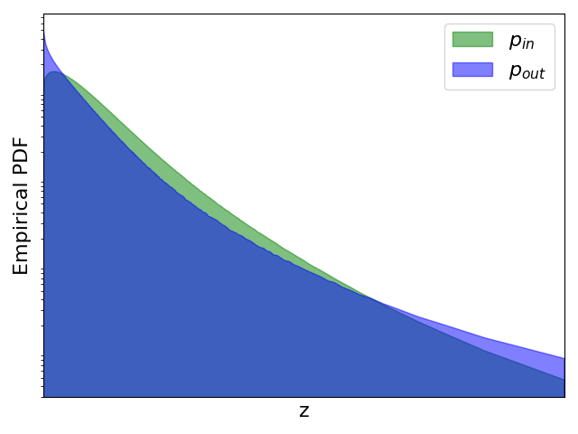
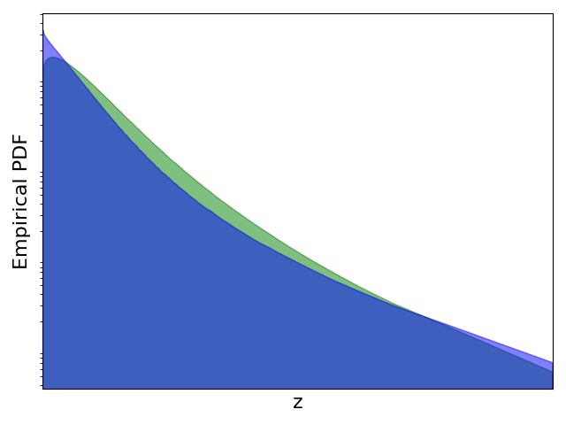
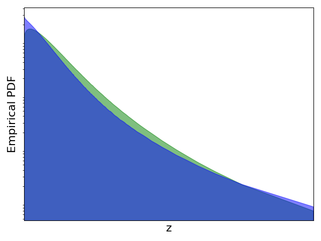
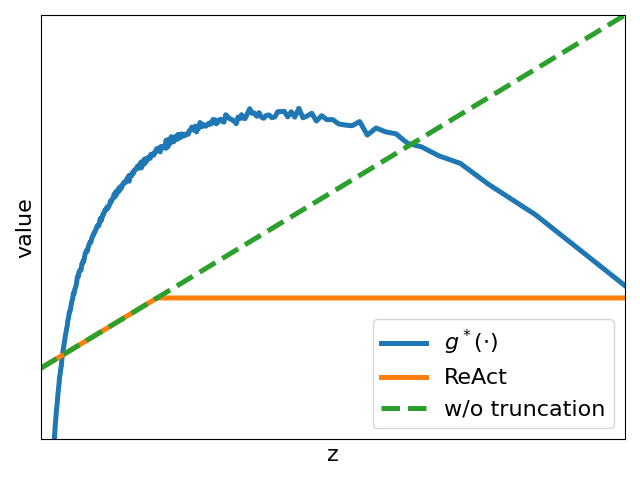
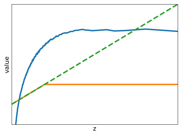
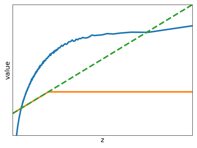
为此，我们将 ImageNet 视为 ID 数据并选择多个 OOD 数据集。 我们首先使用直方图来近似$p_{\text{in}}$和$p_{\text{out}}$的概率密度函数。 然后，我们计算 $g^{\ast }(\cdot )$ 并将其与 ReAct 进行比较，ReAct 的阈值设置为根据 ID 数据估计的激活的第 90^th 百分位，与原始论文 [8 一致]。 实验结果如图1所示。 与没有截断的模型相比，我们观察到 ReAct 抑制了高激活（见图1(d)$\sim$1(f))。 与ReAct不同，最优操作$g^{\ast }(\cdot )$进一步证明了在OOD检测中抑制异常低激活的必要性。 为了模拟此类操作，我们设计了一个名为 VRA 的分段函数：

其中 $\alpha$ 和 $\beta$ 是确定低激活和高激活的两个阈值。 显然，$\alpha =0$和$\beta =\mathrm{\infty }$代表没有激活截断的模型； $\alpha =0$和$\beta >0$表示相当于ReAct的模型。 因此，我们的方法是一个更通用的操作。 由于不同的特征具有不同的分布，因此我们提出了一种自适应调整策略来确定$\alpha$和$\beta$。 具体来说，我们预定义满足的${\eta }_{\alpha }$和${\eta }_{\beta }$。 然后，我们将 ID 数据上估计的激活的 ${\eta }_{\alpha }$-分位数（或 ${\eta }_{\beta }$-分位数）视为 $\alpha$（或 $\beta$) 。 同时，我们观察到$g^{\ast }(\cdot )$放大了图1(d)$\sim$1(f)中的中间激活。 因此，我们提出了 VRA 的另一种变体 VRA+，它进一步引入了一个超参数 $\gamma$ 来控制放大程度：

3实验

3.1实验设置

语料库描述

与之前的工作一致，我们针对不同的 ID 数据集 [8, 10] 考虑不同的 OOD 数据集。 对于 CIFAR 基准测试 [11] 作为 ID 数据，我们使用官方/测试分割作为 ID 数据，并选择六个数据集作为 OOD 数据：纹理 [12]、SVHN [13]、Places365 [14]、LSUN 裁剪 [15]、LSUN 调整大小 [15]、和 iSUN [16]；对于 ImageNet [17] 作为 ID 数据，由于更大的标签空间和更高分辨率的图像，它比 CIFAR 基准更具挑战性。 为了确保ID和OOD之间的类别不重叠，我们从四个数据集中选择一个子集作为OOD数据，与之前的工作[8, 10]一致：iNaturalist [18]、SUN [19]、地点 [14] 和纹理 [12]。

基线

为了验证我们方法的有效性，我们实现了以下最先进的事后策略作为基线：1）MSP [20] 是直接利用最大 softmax 的最基本方法识别 OOD 数据的概率； 2）ODIN [21]使用温度缩放和输入扰动来增加ID和OOD之间的差距； 3）Mahalanobis[22]计算距离最近的类中心的距离作为指标； 4）Energy[23]用理论上保证的Energy分数代替最大softmax概率； 5) ReAct [8] 应用激活截断来去除异常高的激活； 6）KNN [24]利用非参数最近邻距离进行OOD检测； 7) DICE [10] 利用稀疏化来选择最显着的权重； 8) SHE [25]使用现代Hopfield网络[26]中定义的能量函数。

实施细节

我们的方法包含三个用户特定的参数：阈值${\eta }_{\alpha }$和${\eta }_{\beta }$，以及放大程度$\gamma$。 我们从$\{0.5,0.6,0.65,0.7\}$中选择${\eta }_{\alpha }$，从$\{0.8,0.85,0.9,0.95,0.99\}$中选择${\eta }_{\beta }$，从$\{0.2,0.3,0.4,0.5,0.6,0.7\}$中选择$\gamma$ 。 与之前的工作[8]一致，我们使用高斯噪声图像作为超参数调整的验证集。 默认情况下，我们对 CIFAR 使用 DenseNet-101 [27]，对 ImageNet 使用 ResNet-50 [28]。 所有实验均使用 PyTorch [29] 实现，并使用 NVIDIA Tesla V100 GPU 进行。 为了比较不同方法的性能，我们利用了两种广泛使用的 OOD 检测指标：FPR95 和 AUROC。 其中，FPR95衡量ID数据真阳性率为95%时OOD数据的假阳性率； AUROC 测量接受者操作特征曲线下的面积。

3.2实验结果与讨论

主要结果

为了验证我们方法的有效性，我们将基于 VRA 的方法与竞争性事后策略进行比较。 实验结果如表1和表2所示。 我们观察到，我们的方法通常在不同数据集上达到 Top3 性能，并且总体表现最好。 与这些基线不同，我们尝试通过抑制异常低和高激活并放大中间激活来最大化 ID 和 OOD 之间的差距。 这些结果证明了 OOD 检测中此类抑制和放大操作的有效性。 同时，我们观察到 VRA+ 通常优于 VRA，这表明更接近理论最优解的操作通常可以获得更好的性能。

我们还与需要训练的方法进行比较。 MOS [4] 通过训练时正则化解决 OOD 检测问题。 表2中的实验结果表明，我们的方法优于具有相同主干的MOS。 同时，VOS [5] 是一种最新的先进策略，可以合成虚拟异常值以规范训练过程中的决策边界。 根据他们的原始论文，它在 CIFAR-10 上的 AUROC 中达到了 95.33%，在 FPR95 中达到了 22.47%。 在相同的ID数据、OOD数据和网络架构下，我们的方法优于VOS（见表1)。 因此，基于VRA的方法不需要昂贵的训练过程，但可以在OOD检测中获得更好的性能。

表格1： CIFAR 基准测试的主要结果。 在此表中，我们将检测性能与竞争性事后策略进行了比较。 所有方法均根据 ID 数据进行预训练。 我们报告每个数据集的结果以及所有数据集的平均结果。 “FR。”和“非盟”。是 FPR95 和 AUROC 的缩写。 Top3 结果用红色标记，颜色越深表示性能越好。

Method	SVHN		LSUN-C		LSUN-R		iSUN		Textures		Places365		Average
	FR. $\downarrow$	AU. $\uparrow$	FR. $\downarrow$	AU. $\uparrow$	FR. $\downarrow$	AU. $\uparrow$	FR. $\downarrow$	AU. $\uparrow$	FR. $\downarrow$	AU. $\uparrow$	FR. $\downarrow$	AU. $\uparrow$	FR. $\downarrow$	AU. $\uparrow$
ID Dataset: CIFAR-10; Backbone: DenseNet-101 [27]
MSP [20]	47.27	93.48	33.57	95.54	42.10	94.51	42.31	94.52	64.15	88.15	63.02	88.57	48.74	92.46
ODIN [21]	25.29	94.57	04.70	98.86	03.09	99.02	03.98	98.90	57.50	82.38	52.85	88.55	24.57	93.71
Mahalanobis [22]	06.42	98.31	56.55	86.96	09.14	97.09	09.78	97.25	21.51	92.15	85.14	63.15	31.42	89.15
Energy [23]	40.61	93.99	03.81	99.15	09.28	98.12	10.07	98.07	56.12	86.43	39.40	91.64	26.55	94.57
ReAct [8]	41.64	93.87	05.96	98.84	11.46	97.87	12.72	97.72	43.58	92.47	43.31	91.03	26.45	95.30
KNN [24]	13.51	96.68	30.95	93.82	11.37	97.72	10.79	97.91	24.50	95.19	63.88	85.00	25.83	94.39
DICE [10]	25.99	95.90	00.26	99.92	03.91	99.20	04.36	99.14	41.90	88.18	48.59	89.13	20.84	95.25
SHE [25]	28.12	94.72	00.76	99.84	09.73	98.15	10.99	97.95	51.98	83.07	59.35	84.16	26.82	92.98
VRA	18.75	96.68	01.32	99.63	05.80	98.69	05.70	98.69	34.89	93.42	39.98	91.69	17.74	96.47
VRA+	13.54	97.45	02.03	99.56	06.37	98.72	06.15	98.71	27.07	95.03	39.97	91.96	15.85	96.91
ID Dataset: CIFAR-100; Backbone: DenseNet-101 [27]
MSP [20]	81.70	75.40	60.49	85.60	85.24	69.18	85.99	70.17	84.79	71.48	82.55	74.31	80.13	74.36
ODIN [21]	41.35	92.65	10.54	97.93	65.22	84.22	67.05	83.84	82.34	71.48	82.32	76.84	58.14	84.49
Mahalanobis [22]	22.44	95.67	68.90	86.30	23.07	94.20	31.38	89.28	62.39	79.39	92.66	61.39	50.14	84.37
Energy [23]	87.46	81.85	14.72	97.43	70.65	80.14	74.54	78.95	84.15	71.03	79.20	77.72	68.45	81.19
ReAct [8]	83.81	81.41	25.55	94.92	60.08	87.88	65.27	86.55	77.78	78.95	82.65	74.04	65.86	83.96
KNN [24]	23.96	93.99	70.98	73.37	76.34	76.69	70.88	78.58	37.75	87.48	95.20	59.70	62.52	78.30
DICE [10]	54.65	88.84	00.93	99.74	49.40	91.04	48.72	90.08	65.04	76.42	79.58	77.26	49.72	87.23
SHE [25]	41.89	90.61	01.06	99.68	78.18	73.97	72.73	76.14	61.49	76.57	85.33	70.53	56.78	81.25
VRA	70.91	87.46	10.73	98.04	38.52	93.49	38.53	93.42	47.64	90.17	76.39	78.66	47.12	90.21
VRA+	62.64	88.70	19.82	96.33	28.44	95.47	28.72	95.18	40.62	91.57	79.78	76.42	43.34	90.61

表2： ImageNet 上的主要结果。 所有方法均在 ImageNet 上进行预训练。

Method	iNaturalist		SUN		Places		Textures		Average
	FR. $\downarrow$	AU. $\uparrow$	FR. $\downarrow$	AU. $\uparrow$	FR. $\downarrow$	AU. $\uparrow$	FR. $\downarrow$	AU. $\uparrow$	FR. $\downarrow$	AU. $\uparrow$
Backbone: ResNet-50 [28]
MSP [20]	54.99	87.74	70.83	80.86	73.99	79.76	68.00	79.61	66.95	81.99
ODIN [21]	47.66	89.66	60.15	84.59	67.89	81.78	50.23	85.62	56.48	85.41
Mahalanobis [22]	97.00	52.65	98.50	42.41	98.40	41.79	55.80	85.01	87.43	55.47
Energy [23]	55.72	89.95	59.26	85.89	64.92	82.86	53.72	85.99	58.40	86.17
ReAct [8]	20.38	96.22	24.20	94.20	33.85	91.58	47.30	89.80	31.43	92.95
KNN [24]	59.08	86.20	69.53	80.10	77.09	74.87	11.56	97.18	54.32	84.59
DICE [10]	25.63	94.49	35.15	90.83	46.49	87.48	31.72	90.30	34.75	90.78
SHE [25]	34.22	90.18	54.19	84.69	45.35	90.15	45.09	87.93	44.71	88.24
VRA	15.70	97.12	26.94	94.25	37.85	91.27	21.47	95.62	25.49	94.57
VRA+	15.48	97.08	23.50	94.91	34.62	91.79	19.66	96.08	23.31	94.97
Backbone: ResNetv2-101 [28]
MSP [20]	63.69	87.59	79.98	78.34	81.44	76.76	82.73	75.45	76.96	79.54
ODIN [21]	62.69	89.36	71.67	83.92	76.27	80.67	81.31	76.30	72.99	82.56
Mahalanobis [22]	96.34	46.33	88.43	65.20	89.75	64.46	52.23	72.10	81.69	62.02
Energy [23]	64.91	88.48	65.33	85.32	73.02	81.37	80.87	75.79	71.03	82.74
ReAct [8]	49.97	89.80	65.30	87.40	73.12	85.34	80.82	70.53	67.30	83.27
MOS [4]	09.28	98.15	40.63	92.01	49.54	89.06	60.43	81.23	39.97	90.11
VRA	27.26	95.68	34.53	93.27	47.31	90.19	30.69	94.22	34.95	93.34
VRA+	20.81	97.70	32.89	92.68	45.83	90.01	23.88	95.43	30.85	93.71

与评分功能的兼容性

在表 3 中，我们研究了基于 VRA 的方法与不同评分函数（MSP、Energy 和 ODIN）的兼容性。 实验结果表明，我们的方法为所有评分函数带来了性能改进，并且通常比竞争性事后策略获得更好的性能。 这些结果验证了我们的方法在 OOD 检测中的兼容性和有效性。

表3： 与不同评分函数的兼容性。 对于每个 ID 数据集，我们报告其 OOD 数据集的平均结果。 我们对 CIFAR 使用 DenseNet-101 [27]，对 ImageNet 使用 ResNet-50 [28]。

Method	CIFAR-10		CIFAR-100		ImageNet		Average
	FPR95 $\downarrow$	AUROC $\uparrow$	FPR95 $\downarrow$	AUROC $\uparrow$	FPR95 $\downarrow$	AUROC $\uparrow$	FPR95 $\downarrow$	AUROC $\uparrow$
MSP [20]	48.73	92.46	80.13	74.36	66.95	81.99	65.27	82.94
MSP + ReAct	48.00	92.77	77.69	76.22	55.63	87.85	60.44	85.61
MSP + DICE	43.72	92.92	76.86	76.39	67.41	82.24	62.66	83.85
MSP + VRA	42.31	93.50	79.69	75.94	47.09	89.62	56.36	86.35
Energy [23]	26.55	94.57	68.45	81.19	58.41	86.17	51.14	87.31
Energy + ReAct	26.45	94.67	62.27	84.47	31.43	92.95	40.05	90.70
Energy + DICE	20.83	95.24	49.72	87.23	34.75	90.77	35.10	91.08
Energy + VRA	17.74	96.47	53.24	88.74	25.49	94.57	32.16	93.26
ODIN [21]	24.57	93.71	58.14	84.49	56.48	85.41	46.40	87.87
ODIN + ReAct	21.00	95.98	54.17	88.62	42.21	91.28	39.13	91.96
ODIN + DICE	26.05	94.62	61.39	83.83	62.89	84.48	50.11	87.64
ODIN + VRA	17.38	96.52	47.12	90.21	32.75	93.39	32.42	93.37

性能上限分析

我们提出 VRA 和 VRA+ 来近似 OOD 检测的最佳操作。 但是否有必要设计其他函数以获得更好的近似值？ 为了回答这个问题，我们需要揭示$g^{\ast }(\cdot )$是否能够达到上限性能。 估计$g^{\ast }(\cdot )$的核心是估计$p_{\text{in}}$和$p_{\text{out}}$的概率密度函数。 为此，我们考虑两种理想情况：VRA-True和VRA-Fake-True。 在第一种情况下，我们假设所有ID和OOD数据都是预先已知的；在第二种情况下，我们从整个数据集中随机选择 1% 的 ID 和 OOD 数据。 这两种情况都利用直方图来估计 $p_{\text{in}}$ 和 $p_{\text{out}}$ 并使用等式： 13 计算$g^{\ast }(\cdot )$。 考虑到直方图提供了$g^{\ast }(\cdot )$的分段形式，我们直接使用分段函数来表示$g^{\ast }(\cdot )$。 在表4中，我们观察到两种理想情况都可以达到近乎完美的结果。 因此，增加ID和OOD之间差距的$g^{\ast }(\cdot )$可以为OOD检测生成更具区分性的特征。 将来，我们将探索其他可以更好地描述最佳操作以获得更好性能的函数。

表 4： 性能上限分析。 对于每个 ID 数据集，我们报告多个 OOD 数据集的平均结果。 我们对 CIFAR 使用 DenseNet-101 [27]，对 ImageNet 使用 ResNet-50 [28]。

ID	Energy [23]		VRA		VRA-Fake-True		VRA-True
	FPR95 $\downarrow$	AUROC $\uparrow$	FPR95 $\downarrow$	AUROC $\uparrow$	FPR95 $\downarrow$	AUROC $\uparrow$	FPR95 $\downarrow$	AUROC $\uparrow$
CIFAR-10	26.55	94.57	17.74	96.47	13.27	97.75	00.96	99.81
CIFAR-100	68.45	81.19	47.12	90.21	23.62	94.20	01.58	99.69
ImageNet	58.41	86.17	25.49	94.57	13.09	96.89	03.50	99.31

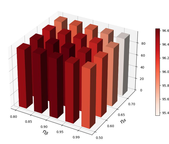
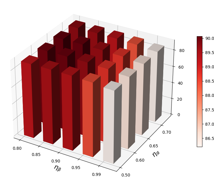
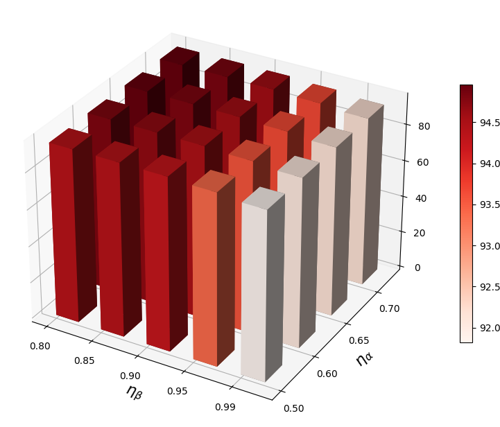
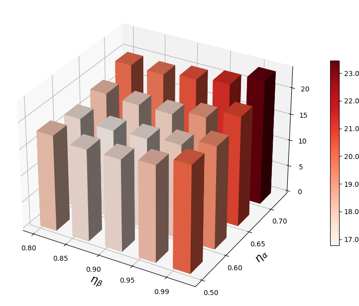
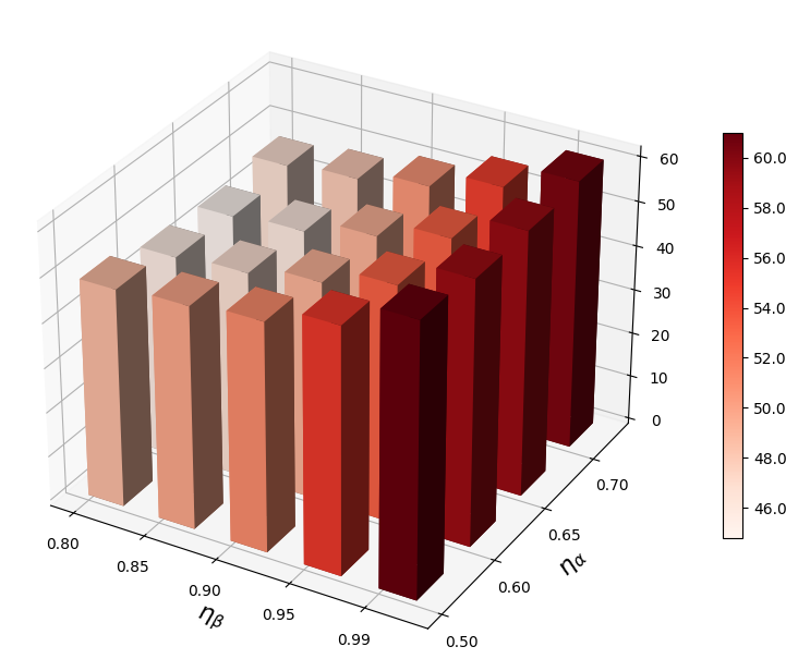
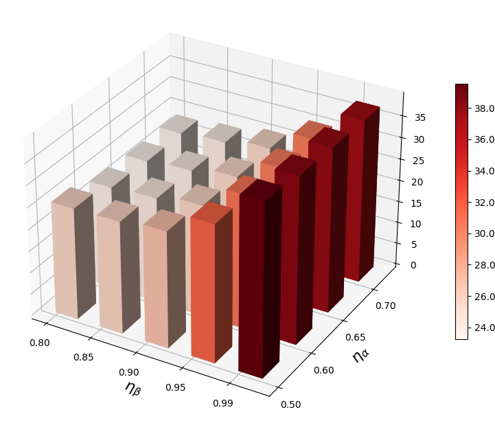
参数敏感性分析

VRA 使用两个超参数(${\eta }_{\alpha }$ 和 ${\eta }_{\beta }$)来自适应调整低激活和高激活的阈值。 在本节中，我们进行参数敏感性分析并揭示它们对 OOD 检测的影响。 在图2中，我们观察到当${\eta }_{\alpha }$和${\eta }_{\beta }$不合适时，我们的方法表现不佳。 较大的 ${\eta }_{\alpha }$ 会抑制太多的低激活，而较大的 ${\eta }_{\beta }$ 则会抑制太少的高激活。 因此，需要为VRA选择合适的${\eta }_{\alpha }$和${\eta }_{\beta }$。

(a) AUROC on CIFAR-10

(b) AUROC on CIFAR-100

(c) AUROC on ImageNet

(d) FPR95 on CIFAR-10

(e) FPR95 on CIFAR-100

(f) FPR95 on ImageNet

图2： 参数敏感性分析。 对于每个 ID 数据集，我们报告多个 OOD 数据集的平均结果。 我们对 CIFAR 使用 DenseNet-101 [27]，对 ImageNet 使用 ResNet-50 [28]。

自适应调整策略的作用

在本文中，我们采用自适应策略来自动确定$\alpha$和$\beta$。 为了验证其有效性，我们将此自适应策略与另一种针对不同特征使用固定 $\alpha$ 和 $\beta$ 的策略进行比较。 为了确定这些超参数，我们使用高斯噪声图像作为验证集，与之前的工作[8]一致。 表5中的实验结果表明我们的自适应策略优于该固定策略。 原因在于不同的特征具有不同的统计分布。 对不同的特征使用固定的阈值会限制OOD检测的性能。

表 5： 自适应调整策略的作用。 我们使用 DenseNet-101 [27] 进行 CIFAR。

ID	Strategy	Hyper-parameters				OOD Performance
		$\alpha$	$\beta$	${\eta }_{\alpha }$	${\eta }_{\beta }$	FPR95 $\downarrow$	AUROC $\uparrow$
CIFAR-10	assign $\alpha$, $\beta$	0.50	1.50	–	–	19.44	96.34
	assign ${\eta }_{\alpha }$, ${\eta }_{\beta }$	–	–	0.60	0.95	17.74	96.47
CIFAR-100	assign $\alpha$, $\beta$	0.50	1.50	–	–	56.35	86.09
	assign ${\eta }_{\alpha }$, ${\eta }_{\beta }$	–	–	0.60	0.95	47.12	90.21

与骨干网的兼容性

在本节中，我们进一步验证我们的方法与不同骨干网的兼容性。 为了公平比较，所有方法都在 ImageNet 上进行预训练，并且我们报告了 ImageNet 的四个 OOD 数据集的平均结果。 与竞争性事后策略相比，表6中的实验结果表明，我们的方法可以在不同网络架构下实现最佳性能。 这些结果验证了我们方法的有效性和兼容性。 同时，我们在表6中观察到一些有趣的现象。 ReAct [8] 指出 ID 和 OOD 之间不匹配的 BatchNorm [30] 统计信息导致模型对 OOD 数据过度自信。 表6中，VGG-16和VGG-16-BN分别指没有和有BatchNorm的模型。 我们观察到，无论有没有 BatchNorm，ReAct 都无法实现比 Energy 更好的性能，这与之前的发现一致[31]。 因此，BatchNorm可能不是模型过度自信的唯一原因，网络架构也很重要。 此外，除了 EfficientNetV2 之外，Energy [23] 总体性能优于 MSP [20]，这也暴露了其兼容性方面的局限性。 未来我们将进行深入分析，揭示这些现象背后的原因。

表 6： 与不同骨干网的兼容性。 所有方法均在 ImageNet 上进行预训练。

Backbone	MSP		Energy		ReAct+Energy		VRA+Energy
	FPR95 $\downarrow$	AUROC $\uparrow$	FPR95 $\downarrow$	AUROC $\uparrow$	FPR95 $\downarrow$	AUROC $\uparrow$	FPR95 $\downarrow$	AUROC $\uparrow$
ResNet-18 [28]	69.70	80.61	58.59	80.40	36.36	92.17	34.87	92.58
ResNet-34 [28]	68.84	81.19	57.20	86.84	32.23	93.08	30.63	93.46
ResNet-50 [28]	66.95	81.99	58.40	86.17	31.43	92.95	25.49	94.57
ResNet-101 [28]	64.70	82.47	54.84	87.29	31.68	93.03	25.80	94.36
ResNet-152 [28]	61.35	83.74	50.39	88.61	26.57	94.22	22.21	95.20
VGG-16 [32]	67.94	81.60	54.33	88.17	67.81	83.68	32.99	92.59
VGG-16-BN [32]	65.92	82.00	50.49	89.03	59.02	86.34	35.12	92.05
EfficientNetV2 [33]	57.57	83.96	75.29	71.10	48.28	88.01	43.81	89.76
RegNet [34]	65.37	82.85	59.46	85.51	34.65	92.53	26.18	94.55
MobileNetV3 [35]	67.99	82.14	60.49	87.80	60.72	87.82	56.65	89.30

4进一步分析

将特征与 logit 输出相结合可以在 OOD 检测中获得更好的性能[36]。 因此，我们设计了VRA的另一种变体VRA++，其评分函数定义为：

${\lambda }_v{\displaystyle \sum _{i=1}^m}g(z_i)+\log {\displaystyle \sum _{i=1}^c}{e}^{l_i},$ (16)

其中 $z_i,i\in [1,m]$ 表示第 $i$ 个特征，$l_i,i\in [1,c]$ 表示第 $i$ 个 logit 输出。 这个评分函数由两项组成：（1）由于我们已经最大化了ID和OOD${𝔼}_{\text{in}}[g(z_i)]-{𝔼}_{\text{out}}[g(z_i)]$之间的差距，因此我们直接使用所有校正特征的总和${\sum }_{i=1}^{m}g(z_i)$作为指标； (2) 我们还计算了 OOD 检测的 logit 输出的能量得分。 这些项目使用平衡因子${\lambda }_v$组合。 与使用分段函数的 VRA 不同，我们进一步测试二次函数 $g(z)=-z^2+{\alpha }_{v}z$ 的性能。 通过选择适当的${\alpha }_v$，该二次函数还可以模拟抑制和放大操作。 最后，我们的评分函数定义为：

$-{\lambda }_v{\displaystyle \sum _{i=1}^m}(z_i^2-{\alpha }_v{z}_i)+\log {\displaystyle \sum _{i=1}^c}{e}^{l_i}.$ (17)

在所有方法中，ViM [36] 是一种结合了特征和 logit 输出的强大策略。 为了与 ViM 进行公平比较，我们使用相同的 ID 数据 (ImageNet)、OOD 数据 (OpenImage-O [36]、Texture [12]、iNaturalist [18]、ImageNet-O [37])和网络架构（BiT [38])。 表7中的实验结果表明VRA++取得了比ViM更好的性能，验证了我们方法的可扩展性和巨大潜力。 同时，VRA++ 通常在所有变体中实现了最佳性能（见表8)。 这些结果进一步证明了在 OOD 检测中结合特征和 logit 输出的必要性。

表 7： VRA++的性能。 所有方法均基于 BiT [38] 并在 ImageNet 上进行预训练。

Method	OpenImage-O		Texture		iNaturalist		ImageNet-O		Average
	FR. $\downarrow$	AU. $\uparrow$	FR. $\downarrow$	AU. $\uparrow$	FR. $\downarrow$	AU. $\uparrow$	FR. $\downarrow$	AU. $\uparrow$	FR. $\downarrow$	AU. $\uparrow$
MSP [20]	73.72	84.16	76.65	79.80	64.09	87.92	96.85	57.12	77.83	77.25
ODIN [21]	72.83	85.64	74.07	81.60	70.75	86.73	96.85	63.00	78.63	79.24
Mahalanobis [22]	64.32	83.10	14.05	97.33	64.95	85.70	70.05	80.37	53.34	86.63
Energy [23]	73.42	84.77	73.91	81.09	74.98	84.47	96.40	63.59	79.68	78.48
ReAct [8]	54.97	88.94	50.25	90.64	48.60	91.45	91.70	67.07	61.38	84.52
ViM [36]	43.96	91.54	04.69	98.92	55.71	89.30	61.50	83.87	41.47	90.91
VRA++	34.94	93.55	05.02	98.76	22.25	96.37	60.45	84.21	30.67	93.22

表8： VRA 变体的比较。 “Net1”和“Net2”指的是ResNet-50和ResNetv2-101。

Method	CIFAR-10		CIFAR-100		ImageNet (Net1)		ImageNet (Net2)
	FPR95 $\downarrow$	AUROC $\uparrow$	FPR95 $\downarrow$	AUROC $\uparrow$	FPR95 $\downarrow$	AUROC $\uparrow$	FPR95 $\downarrow$	AUROC $\uparrow$
VRA	17.74	96.47	47.12	90.21	25.49	94.57	34.95	93.34
VRA+	15.89	96.90	43.31	90.61	23.32	94.96	30.85	93.78
VRA++	15.52	96.87	35.20	91.80	18.63	95.75	25.92	94.60

5相关工作

事后法

事后策略是 OOD 检测的一个重要分支。 由于其易于实施，它们越来越受到研究人员的关注。 其中，MSP[20]是最基本的事后策略，直接利用后验分布的最大值作为指标。 从那时起，研究人员提出了各种事后方法。 例如，ODIN [21] 使用温度缩放和输入扰动来提高 ID 和 OOD 数据的可分离性。 Energy [23] 用理论上保证的能量分数替换了 MSP [20] 中的 softmax 置信度分数。 Mahalanobis [22] 使用距类中心的最小距离来识别 OOD 数据。 KNN [24] 是一种探索 K 最近邻的非参数方法。 最近，研究人员发现模型对 OOD 数据过度自信的原因在于少数神经元的异常高激活。 为了解决这个问题，Dice [10] 使用权重稀疏化，而 ReAct [8] 利用激活截断。 与这些工作不同的是，我们进一步证明异常低的激活也会影响 OOD 检测性能。 这促使我们提出 VRA 来纠正激活函数。

激活函数

激活函数是神经网络的重要组成部分[39, 40]。 此前，研究人员发现，具有 ReLU 激活函数的神经网络对远离训练数据的输入产生异常高的激活，从而损害了已部署系统的可靠性[41]。 为了解决这个问题，ReAct 使用截断操作来纠正激活函数。 在本文中，我们提出了一种更强大的用于 OOD 检测的修正激活函数。 多个基准数据集的实验结果证明了我们方法的有效性。

变分法

变分法常用于求解函数极值。 它在神经网络中最著名的应用是变分自动编码器[42]，它通过权衡重建损失和 Kullback-Leibler 散度来解决函数极值。 它还被应用于其他复杂场景[43]和多模态任务[44]。 在本文中，我们使用变分方法来寻找可以最大化ID和OOD之间差距的操作。

6结论

本文提出了一种称为 VRA 的事后 OOD 检测策略。 从变分方法的角度来看，我们找到了理论上最优的操作来最大化ID和OOD之间的差距。 该操作揭示了在 OOD 检测中抑制异常低和高激活以及放大中间激活的必要性。 因此，我们建议 VRA 来模拟这些抑制和放大操作。 实验结果表明，我们的方法优于现有的事后策略，并且与不同的评分函数和网络架构兼容。 在了解一小部分 OOD 样本的理想情况下，我们可以实现近乎完美的性能，展示了我们方法的强大潜力。 同时，我们验证了自适应调整策略的有效性并揭示了不同超参数的影响。

在本文中，我们将${\max }_g{𝔼}_{\text{in}}[g(z)]-{𝔼}_{\text{out}}[g(z)]$视为从ReAct导出的核心目标函数，将${\min }_g{𝔼}_{\text{in}}[{(g(z)-z)}^2]$视为正则化项。 然而，可能存在更好的正则化项，既能保证最优解的存在，又能保证最优解的表达易于实现，并具有良好的可解释性。 因此，我们将探索 OOD 检测的其他正则化项。 同时，本文使用简单的分段函数来逼近复杂的最优操作。 未来，我们将探索其他能够更好地描述最优操作的函数形式。 我们还将进行深入分析，揭示 BatchNorm 和不同主干网对 OOD 检测的影响。