通过跨模态特征映射进行多模态工业异常检测
摘要
本文探讨了工业多模式异常检测 (AD) 任务,该任务利用点云和 RGB 图像来定位异常。 我们引入了一种新颖的轻量级快速框架,该框架学习将标称样本上的特征从一种模态映射到另一种模态。 在测试时,通过查明观察到的特征和映射的特征之间的不一致来检测异常。 大量实验表明,我们的方法在 MVTec 3D-AD 数据集的标准和少样本设置中实现了最先进的检测和分割性能,同时比以前的多模态 AD 方法实现更快的推理并占用更少的内存。 此外,我们提出了一种层剪枝技术来提高内存和时间效率,同时稍微牺牲性能。
1简介
工业异常检测 (AD) 旨在识别产品中的异常特征或缺陷,是质量检查流程中的重要组成部分。 由于异常现象的稀有性和不可预测性,收集数据来举例说明异常现象具有挑战性。 因此,大多数工作都集中在无监督方法,即。,仅在没有缺陷的样本(也称为标称样本)上训练的算法。 目前,大多数现有的 AD 方法都是针对分析 RGB 图像。 然而,在许多工业环境中,仅根据彩色图像很难有效识别异常,例如。,因为不同的光照条件容易导致错误检测,并且表面偏差可能会导致错误检测。不会出现不太可能的颜色。 部署 3D 传感器获取的彩色图像和表面信息可以解决上述问题并显着改善 AD。
最近,由于引入了 3D 异常检测基准数据集,例如 MVTec 3D-AD [5] 和 Eyecandies [6],研究人员开始探索新的途径。 事实上,两者都为所有数据样本提供 RGB 图像以及像素配准的 3D 信息,从而促进了新的多模态 AD 方法的开发[42,17,36]。 BTF [17] 和 M3DM [42] 等无监督多模态 AD 方法依赖于多模态特征的大型存储库。 它们实现了出色的性能(图 1中的 AUPRO@30% 指标),但代价是大量内存需求和缓慢的推理 ( 图 1)。 特别是,M3DM 通过利用在大型数据集(i.e.、ImageNet 和 Shapenet)上进行自监督训练的冻结特征提取器(分别针对 2D 和 3D 特征)而优于 BTF。
另一种最近的多模态方法 AST [36] 遵循有利于更快架构的师生范式(图 1)。 然而,AST 并未利用 3D 数据的空间结构,而是将此信息用作 2D 网络架构中的附加输入通道。 与 M3DM 和 BTF 相比,这导致性能较差(图 1)。
在本文中,我们提出了一种新的范式来利用从不同模态提取的特征之间的关系并改进多模态 AD。 图2中描述的我们方法背后的核心思想是学习两个crossmodal映射函数, 和 ,分别位于冻结 2D 和 3D 特征提取器 和 的潜在空间之间。 因此,给定 2D 提取器计算的 2D 特征, 学习预测 3D 提取器计算的相应 3D 特征,同样, 学习预测 2D 特征给定的 3D 特征。 当我们学习标称数据上的两个映射函数时,我们期望它们能够捕获好样本特有的跨模态关系,而异常,就其本质而言,实现了当时看不见的映射,例如从未与某个特定特征结合观察到的二维特征3D 特征,反之亦然。 因此,在推理时,我们通过估计和聚合两个冻结提取器提供的实际特征与跨模态映射函数预测的特征之间的差异来计算异常图。
该框架能够有效且高效地实现多模式自动驾驶。 事实上,没有明显的、琐碎的解决方案可以导致跨模式映射网络泛化到有缺陷的样本。 例如,由于输入和输出特征是从不同的模态中提取的,网络无法学习恒等映射,这可能发生在以前基于重建的 AD 方法[23]中。 此外,正如我们将在Sec. 3中讨论的那样,对标称数据中的 2D 和 3D 特征之间的关系进行建模可以对各种异常。 最后,特征映射函数可以实现为轻量级神经网络,例如小型且浅层的 MLP。 这可以在有限的内存占用下产生非常快速的推理。
如图图1所示,我们基于跨模态映射函数的新颖AD方法在MVTec 3D上实现了最先进的性能- AD,优于基于内存库的最佳资源密集型方法(我们的方法与 M3DM),同时提供更快的推理速度。 此外,我们还观察到,学习来自冻结提取器的较浅层的特征之间的映射可以在内存需求和推理速度方面产生巨大的收益,而对我们方法的有效性的影响相对有限。 因此,我们可以修剪 2D 和 3D 特征提取器的最深层,以获得我们框架的 Small 和 Tiny 变体(图 5)。 t3> 1:Ours-S、Ours-T),需要更少的内存并且运行速度更快。 值得注意的是,Small 架构仍然在 MVTec 3D-AD 上提供最先进的性能,同时与完整模型相比,所需内存不到一半,而 Tiny 架构运行速度几乎是 BTF 和 AST 的两倍,并且性能优于 BTF 和 AST。 最后,我们指出,即使使用一些标称样本,我们的方法也可以进行训练。 为了在这种具有挑战性的场景中正确评估我们的方法,我们从 MVTec 3D-AD 构建了第一个少样本多模态 AD 基准,我们注意到我们的方法实现了最先进的异常分割性能。
代码将在发布后发布。 我们的贡献可概括如下:
-
•
我们提出了一种基于跨模态映射特征的无监督多模态 AD 的新颖框架;
-
•
通过使用冻结 2D 和 3D 提取器提取的特定模态特征,我们在 MVTec 3D-AD 上获得了最先进的检测和分割性能,同时达到了与 Eyecandies 上最先进的性能相当的性能。
-
•
我们的方法能够进行非常快速的推理,并且比最先进的解决方案需要更少的内存。
-
•
我们在建立在 MVTec 3D-AD 之上的拟议少样本 AD 基准上达到了最先进的性能;
-
•
我们制定了一种在不过度影响性能的情况下修剪网络的策略。 通过这种方式,我们可以实现显着更快的推理并节省大量内存。
2相关工作
无监督图像异常检测。 分析 RGB 图像的无监督 AD 方法[23]可以分为两大类。 第一个背后的总体思想是学习如何使用自动编码器 [2, 49, 18, 33] 重建标称样本的图像,修复 [28] ,或扩散模型[43]。 然后,在测试时,由于训练的模型无法正确重建异常图像,因此可以通过分析输入图像和重建图像之间的差异来计算每像素异常图。 第二类方法侧重于深度神经网络定义的特征空间[31, 46, 50, 40, 47, 22, 45, 24, 48, 35, 32, 15, 10, 12]. 在这些技术中,师生[4,41,7,38,13]是AD的典型策略之一。 在训练过程中,教师模型从名义样本中提取特征,并将知识提炼到学生模型中。 在测试时,通过分析教师和学生计算的特征之间的差异来检测异常。 不同的是,深度特征重建(DFR)[44]根据从标称样本中提取的特征来训练自动编码器。 然后,与图像重建方法类似,它通过分析重建特征与原始特征之间的差异来识别测试样本中的异常。 有效的通用特征提取器[8,25,16](也称为基础模型)的可用性不断增加,引起了人们对部署特征的异常检测方法的兴趣由冻结模型[34,11,1]提取。 在训练时,由冻结提取器根据标称样本计算出的特征存储在存储器中。 在推理时,将冻结模型从输入图像中提取的特征与存储在库中的特征进行比较,以识别异常。 这些方法实现了卓越的性能,但代价是推理速度较慢(因为从输入图像中提取的每个特征向量都必须与存储在存储体中的所有标称特征向量进行比较)以及显着的内存占用(因为较大的存储体可以更好地捕获可变性)名义特征。
多模式 RGB-3D 异常检测。 多模态方法利用 RGB 图像和 3D 数据来增强异常检测的稳健性和有效性。 继基于图像的 AD 基准测试 [3] 方面颇具影响力的工作之后,最近的一篇论文 [5] 介绍了 MVTec 3D-AD 数据集,以及包括多个基线的实验验证,例如基于 GAN 和变分模型(即.、VAE)的分布映射技术,以及自动编码器。 这些基线模型在由体素网格或深度图表示的 3D 数据上进行训练,并将 RGB 信息合并为附加输入通道。 [36]中提出的方法由旨在处理RGB-D数据的非对称学生-教师方法(AST)组成,其中两个网络具有不同的架构以防止对异常样本的过度泛化。 受 PatchCore [34] 的启发,BTF [17] 研究了使用内存库进行 3D 异常检测。 作者建议将 3D 特征添加到冻结卷积模型 (Wide ResNet-50) 提供的 2D 特征中,以增强异常检测性能。 他们测试了多个 3D 特征,并使用从点云[37]中提取的手工制作的描述符获得了最佳结果。 M3DM [42] 通过采用丰富且独特的 2D 和 3D 特征来改进 BTF,这些特征是通过在大型数据集上进行自我监督训练的基于 Transformer 的冻结基础模型提取的。 特别是,他们使用 DINO [8] 和 Point-MAE [26] 分别提取 2D 和 3D 特征。 作者还提出了一种学习函数,将 2D 和 3D 特征融合为存储在内存库中的多模态特征以及根据各个模态计算的特征。 由于强大的 2D、3D 和多模态功能的联合部署,它们实现了卓越的性能,为 MVTec 3D-AD 设定了最高标准。 然而,对大型功能库的依赖使得 M3DM 在内存和时间方面过于昂贵(图 1)。 与 M3DM [42] 类似,我们的方法部署了由基于 Transformer 的冻结模型计算得出的引人注目的 2D 和 3D 特征。 然而,我们没有使用任何存储库,而是提出了一种新颖的跨模式特征映射范例,可以通过两个轻量级神经网络来实现。 使用与 M3DM [42] 相同的特征提取器,我们在 MVTec 3D-AD 上实现了更好的性能,同时需要更少的内存并且运行速度显着加快(图 1)。
3方法
我们的多模态 AD 方法依赖于学习从标称样本中提取的特征之间的跨模态映射,以根据预测和观察到的特征之间的差异查明异常。 如图图 2所示,这是通过(i)一对冻结特征提取器; (ii) 一对特征映射网络; (iii) 聚合模块。
3.1特征提取
我们管道中的第一步涉及提取 2D 图像中表示为 的每个像素以及表示为 的 3D 点云中每个点的特征。 正如Sec. 1中所解释的,在我们的框架中,两个特征提取器都在大型外部数据集上进行训练并冻结,即.,它们的权重永远不会更新。
2D 特征提取和插值。 给定尺寸为 的图像 ,我们使用 2D 特征提取器对其进行处理,表示为 ,生成尺寸为 由于尺寸和小于原始和,我们应用双线性上采样操作来获得,这是维度为的特征图,从而获得每个像素位置的特征向量。
3D 特征提取和插值。 给定一个尺寸为 的点云,我们使用 3D 特征提取器 对其进行处理,得到一组尺寸为 的 特征向量。 每个特征向量 都与原始点云 内的特定点相关联。 事实上,许多 3D 特征提取器(例如。、[26])不会估计每个输入点的特征,而只会估计其中的一个子集,即。,。因此,为了获得云中每个点 的特征向量 ,我们遵循类似于 [42] 的过程。 这里,被计算为三个特征向量的加权和,这三个特征向量在提取的中与 这样,我们就获得了,一组大小为的插值特征向量。
特征对齐。 根据多模态 AD [5, 6] 中的标准设置,我们假设像素配准的 3D 数据和图像。 因此,我们知道与每个 3D 点相关的相应像素位置。 由于和已经被插值以匹配原始图像和点云分辨率,我们可以将投影到2D图像平面,获得,维度的特征图。 在此过程中,我们将没有相应 3D 特征的像素位置处的矢量设置为零。 最后,我们在 上应用 平滑内核。 在此过程结束时,我们获得 和 ,两个在像素级别对齐的特征图。
3.2 跨模态特征映射
获得 和 后,我们部署两个特征映射函数,作为轻量级 MLP 实现, 和 。 将大小为 的特征向量映射到另一个大小为 的特征向量,而 则相反。 每个网络预测一种模态的特征与另一种模态的特征,独立处理每个像素位置。 因此,给定像素位置 以及相应的 2D 和 3D 特征 和 ,我们可以获得另一种模态的预测特征:
| (1) |
当处理没有关联 3D 点的像素位置时,我们将相应的预测特征设置为零。 通过处理所有像素,我们分别获得维度为 和 的预测特征图 。
训练。 在训练时,通过最小化根据两种模态的输入数据计算出的特征图之间的余弦距离,对数据集的所有标称样本联合优化 和 那些。 因此,每像素损失为:
| (2) |
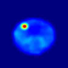
基本原理。 正如Sec.1中所指出的,这种新颖的范式对各种异常现象提供了高度的敏感性。 让我们用图3中提供的玩具示例来概念化这个属性。 在训练时(左上),我们观察到平坦 3D 表面上的红色 2D 图案和弯曲 3D 表面上的蓝色 2D 图案: 和 学习预测提取的特征之间的关系从这些数据中。 在推理时,如果曲面(右上角)上出现异常(例如。、黄色 2D 图案), 会预测 2D 特征对应于蓝色图案,而观察到的 2D 特征涉及黄色图案。 此外, 接收训练时未见过的输入特征,这不太可能产生实际曲面的 3D 特征作为输出。 因此,我们的方法感知 2D 和 3D 特征的预测和观察之间的差异。 类似的考虑也适用于异常 3D 表面上的标称 2D 图案(左下):两种预测均与观察结果不一致。 当两种模态都表现出异常时也是这种情况(未在图 3中显示):两个输入在训练时都看不见,因此两个跨模式预测不太可能与观察结果相符。 最后,我们强调强制执行多模态 AD 的情况:各个模态符合名义分布,但它们的共现是异常的。 这可以通过曲面上的红色图案(右下)来举例说明:同样, 输出平坦面片的 3D 特征, 输出蓝色面片的 2D 特征,两个预测都与观察结果不一致。
值得指出的是,由于标称样本的可变性,2D 和 3D 特征之间的映射可能不唯一。 例如,在图3中,可能同时存在红色的平面和曲面,并且这个一对一许多映射使得很难学习与红色斑块的2D特征相关联的正确3D特征。 因此,当出现红色补丁时, 可能会预测错误的 3D 特征或不太可能的 3D 特征,从而导致预测的 3D 特征与观察到的 3D 特征之间存在差异。 然而,由于映射是多对一,可以预测红色斑块的2D特征。 因此,只有当两个预测与观察结果不一致时,我们才可以通过查明异常来避免错误检测。 当然,由于标称样本的变异性更高,我们还可能面临一对多映射,例如。,再次考虑图3,弯曲3D块上的蓝色和红色图像块。 在这种情况下,当在曲面上呈现红色斑块时,可能会错误地预测平坦斑块的特征,而可能会错误地预测蓝色斑块的特征,最终导致由于两个预测与观察结果不一致而导致错误的异常检测。
尽管如此,在我们的框架中,我们可以通过利用 Transformer 架构提供的高度上下文化的 2D 和 3D 特征来解决跨模式的潜在一对多特征映射问题[8, 26 ]。 事实上,上下文化 2D 特征,例如.,描述了被蓝色和紫色斑块包围的红色斑块,往往对应于特定的上下文化 3D 特征,例如.,表示位于波纹表面区域右侧的平坦斑块。 换句话说,Transformers 提取的高度上下文化的 2D 和 3D 特征不太容易实现一对多跨模态映射。 出于上述原因,我们为 和 使用 Transformer。
3.3聚合
在推理时,测试样本被转发到特征提取和映射网络以获得两对提取和预测的特征图。 在对所有单独的特征向量进行归一化之后,通过差异函数逐像素比较提取的图和预测的图,以获得特定于模态的异常图:
| (3) |
我们使用欧几里德距离作为差异。
然后使用聚合函数组合上述异常图,得到最终的异常图。 正如Sec. 3.2在Fig. 3的帮助下讨论的>,只有当两个预测与观察结果不一致时才精确定位异常,可以对各种异常提供高灵敏度,并对错误检测具有良好的鲁棒性。 因此,我们使用逐像素乘积作为聚合函数:,它可以被认为是逻辑与:只有当模态和模态都如此时,任何像素位置的异常分数才很高。具体分数,即。,异常检测必须通过两种方式得到证实。
聚合异常图最终通过 的高斯核进行平滑,类似于常见做法 [42, 34, 11]。 获得执行样本级异常检测所需的全局异常分数作为异常图的最大值。
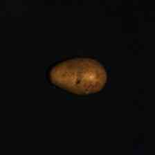
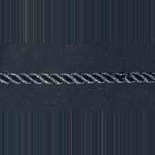
| Method | Bagel | Cable Gland | Carrot | Cookie | Dowel | Foam | Peach | Potato | Rope | Tire | Mean | |
|---|---|---|---|---|---|---|---|---|---|---|---|---|
| I-AUROC | DepthGAN [5] | 0.538 | 0.372 | 0.580 | 0.603 | 0.430 | 0.534 | 0.642 | 0.601 | 0.443 | 0.577 | 0.532 |
| DepthAE [5] | 0.648 | 0.502 | 0.650 | 0.488 | 0.805 | 0.522 | 0.712 | 0.529 | 0.540 | 0.552 | 0.595 | |
| DepthVM [5] | 0.513 | 0.551 | 0.477 | 0.581 | 0.617 | 0.716 | 0.450 | 0.421 | 0.598 | 0.623 | 0.555 | |
| VoxelGAN [5] | 0.680 | 0.324 | 0.565 | 0.399 | 0.497 | 0.482 | 0.566 | 0.579 | 0.601 | 0.482 | 0.517 | |
| VoxelAE [5] | 0.510 | 0.540 | 0.384 | 0.693 | 0.446 | 0.632 | 0.550 | 0.494 | 0.721 | 0.413 | 0.538 | |
| VoxelVM [5] | 0.553 | 0.772 | 0.484 | 0.701 | 0.751 | 0.578 | 0.480 | 0.466 | 0.689 | 0.611 | 0.609 | |
| BTF [17] | 0.918 | 0.748 | 0.967 | 0.883 | 0.932 | 0.582 | 0.896 | 0.912 | 0.921 | 0.886 | 0.865 | |
| AST [36] | 0.983 | 0.873 | 0.976 | 0.971 | 0.932 | 0.885 | 0.974 | 0.981 | 1.000 | 0.797 | 0.937 | |
| M3DM [42] | 0.994 | 0.909 | 0.972 | 0.976 | 0.960 | 0.942 | 0.973 | 0.899 | 0.972 | 0.850 | 0.945 | |
| Ours | 0.994 | 0.888 | 0.984 | 0.993 | 0.980 | 0.888 | 0.941 | 0.943 | 0.980 | 0.953 | 0.954 | |
| AUPRO@30% | DepthGAN [5] | 0.421 | 0.422 | 0.778 | 0.696 | 0.494 | 0.252 | 0.285 | 0.362 | 0.402 | 0.631 | 0.474 |
| DepthAE [5] | 0.432 | 0.158 | 0.808 | 0.491 | 0.841 | 0.406 | 0.262 | 0.216 | 0.716 | 0.478 | 0.481 | |
| DepthVM [5] | 0.388 | 0.321 | 0.194 | 0.570 | 0.408 | 0.282 | 0.244 | 0.349 | 0.268 | 0.331 | 0.335 | |
| VoxelGAN [5] | 0.664 | 0.620 | 0.766 | 0.740 | 0.783 | 0.332 | 0.582 | 0.790 | 0.633 | 0.483 | 0.639 | |
| VoxelAE [5] | 0.467 | 0.750 | 0.808 | 0.550 | 0.765 | 0.473 | 0.721 | 0.918 | 0.019 | 0.170 | 0.564 | |
| VoxelVM [5] | 0.510 | 0.331 | 0.413 | 0.715 | 0.680 | 0.279 | 0.300 | 0.507 | 0.611 | 0.366 | 0.471 | |
| BTF [17] | 0.976 | 0.969 | 0.979 | 0.973 | 0.933 | 0.888 | 0.975 | 0.981 | 0.950 | 0.971 | 0.959 | |
| AST [36] | 0.970 | 0.947 | 0.981 | 0.939 | 0.913 | 0.906 | 0.979 | 0.982 | 0.889 | 0.940 | 0.944 | |
| M3DM [42] | 0.970 | 0.971 | 0.979 | 0.950 | 0.941 | 0.932 | 0.977 | 0.971 | 0.971 | 0.975 | 0.964 | |
| Ours | 0.979 | 0.972 | 0.982 | 0.945 | 0.950 | 0.968 | 0.980 | 0.982 | 0.975 | 0.981 | 0.971 |
| Method | Bagel | Cable Gland | Carrot | Cookie | Dowel | Foam | Peach | Potato | Rope | Tire | Mean |
|---|---|---|---|---|---|---|---|---|---|---|---|
| BTF [17] | 0.428 | 0.365 | 0.452 | 0.431 | 0.370 | 0.244 | 0.427 | 0.470 | 0.298 | 0.345 | 0.383 |
| AST [36] | 0.388 | 0.322 | 0.470 | 0.411 | 0.328 | 0.275 | 0.474 | 0.487 | 0.360 | 0.474 | 0.398 |
| M3DM [42] | 0.414 | 0.395 | 0.447 | 0.318 | 0.422 | 0.335 | 0.444 | 0.351 | 0.416 | 0.398 | 0.394 |
| Ours | 0.459 | 0.431 | 0.485 | 0.469 | 0.394 | 0.413 | 0.468 | 0.487 | 0.464 | 0.476 | 0.455 |
3.4层剪枝
我们的解决方案[8, 26]中使用的特征提取器基于由层组成的Transformer编码器。 不同层特征之间的区别因素在于应用于原始输入的自注意力处理程度不同。 随着输入特征下降到编码器层,它们表现出更强的上下文化。 我们观察到,学习冻结提取器较浅层的特征之间的映射可以在内存需求和推理速度方面产生显着的收益,而对有效性的影响有限。 因此,如图图4所示,我们在特定层修剪两个特征提取器的层以获取需要更少内存且运行速度更快的变体。
4实验设置
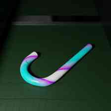
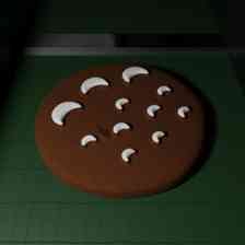
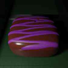
数据集和指标。 我们在两个多模式 AD 基准上评估我们的框架。 MVTec 3D-AD [5] 包含 类工业对象,总共 个训练样本、 个验证样本和 测试样本。 Eyecandies [6] 是一个合成数据集,具有工业传送带场景中 类食品的逼真图像。 它包含 训练样本、 验证样本和 测试样本。 两个数据集都提供每个样本的 RGB 图像以及像素配准的 3D 信息。 因此,我们在每个像素位置都有与 坐标配对的 RGB 信息。 我们采用 MVTec 3D-AD 提出的评估指标。 因此,我们通过根据全局异常得分计算的接收器算子曲线下面积(I-AUROC)来评估图像异常检测性能。 我们通过接收器算子曲线下的像素级面积(P-AUROC)和每区域重叠下的面积(AUPRO)来估计异常分割性能。 之前的所有工作都采用 作为误报率(FPR)积分阈值来计算 AUPRO。 我们认为对于实际工业应用来说,这样的值通常可能过于宽松,从而导致过多的误报。 因此,我们还根据更严格的阈值来计算AUPRO。 我们将积分阈值 和 的 AUPRO 分别表示为 AUPRO@30% 和 AUPRO@1%。 我们在补充材料中报告了带有附加阈值的结果。
实施细节。 我们采用与 M3DM [42] 相同的冻结 Transformer 来实现 和 特征提取器,即。,DINO ViT-B/8 [21, 8] 在 ImageNet [14] 和 Point-MAE [26] 上训练> 分别在 ShapeNet [9] 上进行训练。 因此,处理 RGB图像并输出特征图,这些特征图在馈送到之前被双线性上采样到 的功能。 处理通过 FPS [29] 获得的 组 点,产生维度为 如 Sec. 3.1所述,这些特征在输入到 之前,会被内插并对齐到 中。
和 都仅包含三个线性层,除了最后一层之外,每个层都后面跟着 GeLU 激活。 每层的单元数为 的 和 的 。 使用 Adam [19] 联合训练两个网络 纪元,学习率为 。
如 [17, 42, 36] 中所做的那样,我们在 3D 点云上使用 RANSAC 拟合平面,如果到平面的距离小于 ,则将点视为背景>。 输入中的点云中的背景点被丢弃。 此过程可加速训练和推理期间 3D 特征的处理,并减轻异常地图中的背景噪声。
此外,如Sec.3.4中所述,为了获得框架的更轻版本,我们在层修剪了两个特征提取器等于、、,获得Tiny、Small和Medium 架构称为 Ours-T、Ours-S 和 Ours-M。
我们使用我们的代码和其他多模式 AD 方法作者的原始代码在单个 NVIDIA GeForce RTX 4090 上进行了实验。
5实验
我们在这里报告评估我们提案的实验。
| Method | I-AUROC | P-AUROC | AUPRO@30% | AUPRO@1% |
|---|---|---|---|---|
| AST [36] | 0.758 | 0.902 | 0.878 | 0.224 |
| M3DM [42] | 0.897 | 0.977 | 0.882 | 0.331 |
| Ours | 0.881 | 0.974 | 0.887 | 0.335 |
|
|
|
|
|
|||||||||||||||||||||||||||||||||||||||||||||||||||||||||||||||||||||||||||||||||||||||||||||||||||||
|---|---|---|---|---|---|---|---|---|---|---|---|---|---|---|---|---|---|---|---|---|---|---|---|---|---|---|---|---|---|---|---|---|---|---|---|---|---|---|---|---|---|---|---|---|---|---|---|---|---|---|---|---|---|---|---|---|---|---|---|---|---|---|---|---|---|---|---|---|---|---|---|---|---|---|---|---|---|---|---|---|---|---|---|---|---|---|---|---|---|---|---|---|---|---|---|---|---|---|---|---|---|---|---|---|---|
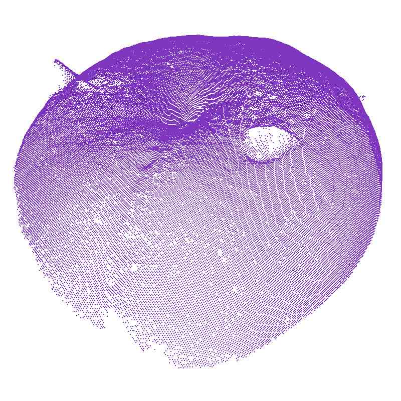
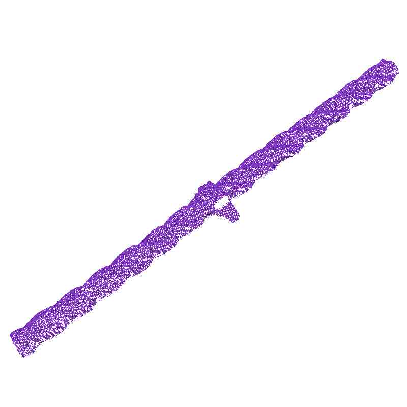
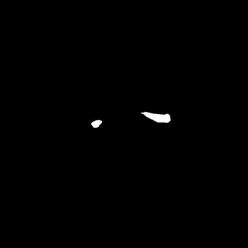
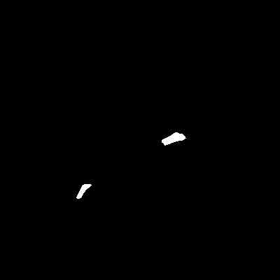
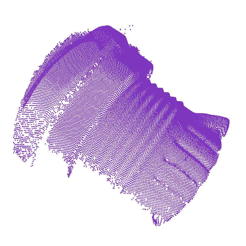
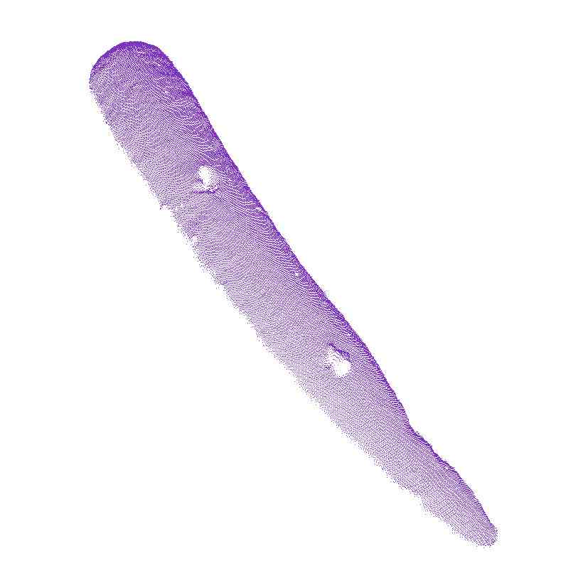
| Bagel | Carrot | Dowel | Peach | Rope | |
|---|---|---|---|---|---|
|
RGB |
 |
 |
 |
 |
 |
|
PC |
 |
 |
 |
 |
 |
|
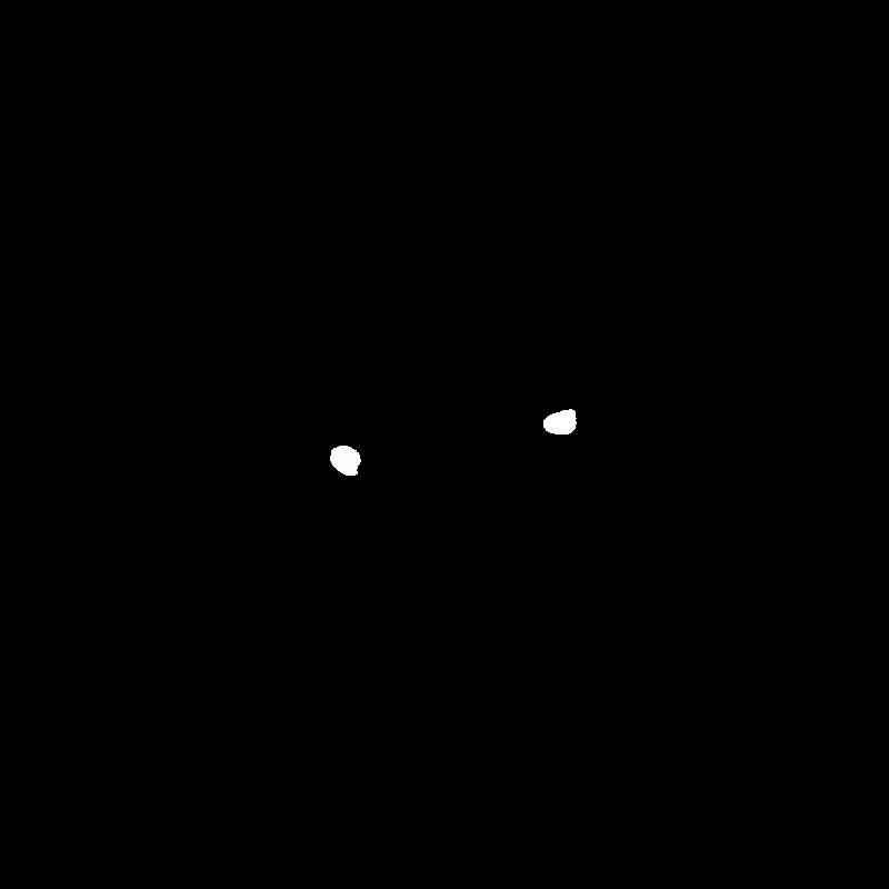
GT |
 |
 |
 |
 |
 |
|
M3DM |
 |
 |
 |
 |
 |
|
Ours |
 |
 |
 |
 |
 |
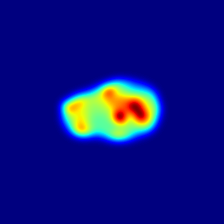
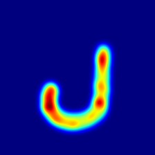
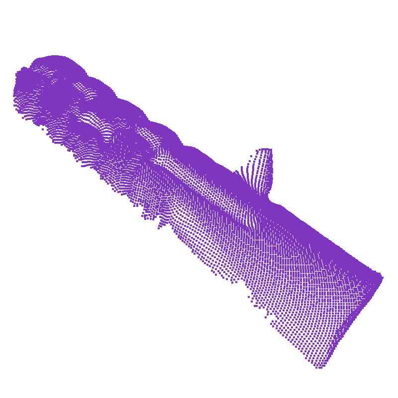
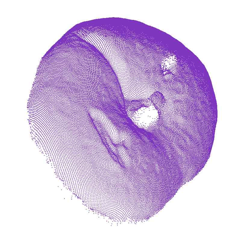
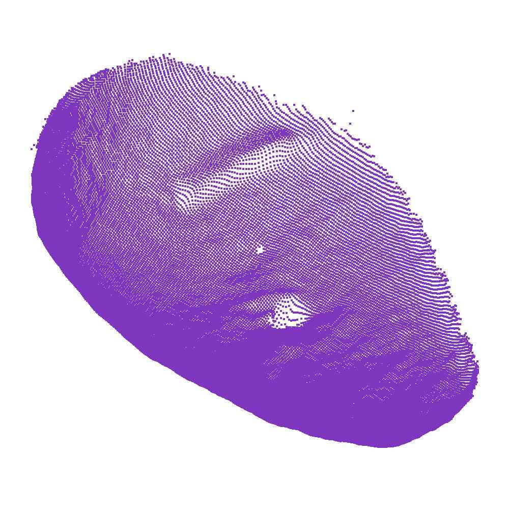
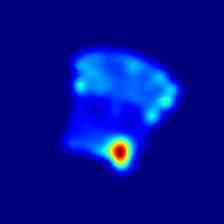
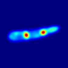
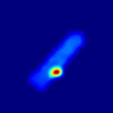
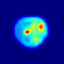
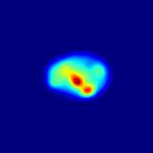
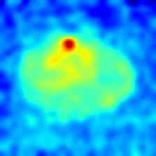
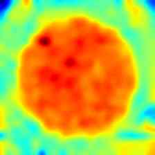
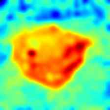
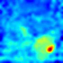
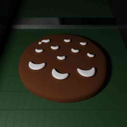
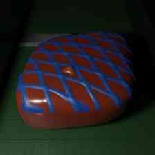
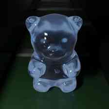
异常检测和分段。 按照[42]的设置,我们评估了 MVTec 3D-AD 和 Eyecandies 上的提案,并在 选项卡。 1, 选项卡。 2 和 选项卡。 3. 我们的方法在 MVTec 3D-AD 上的检测和分割方面取得了最佳结果,在所有三个平均指标(即 I-AUROC、AUPRO@30% 和 AUPRO@1)上均优于之前最先进的方法 M3DM %,以及大多数单独类别。 之间的比较 选项卡。 1 和 选项卡。 2 展示了当评估在可容忍的 FPR 方面设定了更具挑战性的标准时,当前 AD 方法的性能如何显着下降。 正如Sec. 4中提到的,我们相信这样的挑战更符合许多实际工业AD应用的要求。 因此,我们认为 MVTec 3D-AD 基准远未饱和,多模态 AD 还存在巨大的改进空间。 至于养眼糖果, 选项卡。 3,我们实现了与 M3DM 相当的性能,每种方法都有两个获胜指标。 此外,我们强调 P-AUROC 指标似乎几乎饱和,而在 Eyecandies 中,AUPRO@1% 指标也有很大的改进空间。 在图 5中,我们展示了 MVTec 3D-AD 数据集的一些定性结果。 与 M3DM 相比,我们的方法提供了非常清晰的异常图,相对于地面实况缺陷分割定位良好,从而在 AUPRO@1% 方面产生了更大的性能差距。 补充材料中报告了更广泛的定性结果。
| Method | Frame Rate | Memory | I-AUROC | P-AUROC | AUPRO@30% | AUPRO@1% |
|---|---|---|---|---|---|---|
| BTF [17] | 3.197 | 381.06 | 0.865 | 0.992 | 0.959 | 0.383 |
| AST [36] | 4.966 | 463.94 | 0.937 | 0.976 | 0.944 | 0.398 |
| M3DM [42] | 0.514 | 6526.12 | 0.945 | 0.992 | 0.964 | 0.394 |
| Ours | 21.755 | 437.91 | 0.954 | 0.993 | 0.971 | 0.455 |
| Ours-M | 24.146 | 295.81 | 0.960 | 0.994 | 0.972 | 0.459 |
| Ours-S | 24.527 | 211.09 | 0.948 | 0.994 | 0.972 | 0.451 |
| Ours-T | 42.818 | 48.12 | 0.899 | 0.990 | 0.961 | 0.419 |
异常检测和分割样本较少。 在相关工业场景中,收集大量名义样本的成本极其昂贵,甚至不可行。 因此,AD 方法的一个理想特性是能够仅通过少数样本对标称数据的分布进行建模。 为了解决这种情况,我们基于 MVTec 3D-AD 数据集定义了少样本多模态 AD 的第一个基准。 我们从每个类别中随机选择 5、10 和 50 个训练图像作为数据。 我们在这些样本上训练了最好的多模态方法,BTF [17]、M3DM [42] 和 AST [36],并进行测试将它们放在整个 MVTec 3D-AD 测试集上,报告结果 选项卡。 4. 至于检测,我们的方法实现了与 M3DM [42] 相当的 I-AUROC,同时优于其他方法。 我们在所有少样本设置中获得了所有指标(P-AUROC、AUPRO@1% 和 AUPRO@30%)的最佳分割性能,显着改善了最具挑战性的分割指标(5 次拍摄时+0.052 AUPRO@1%) )。 这些结果表明,我们的框架甚至可以从一些名义样本中学习一般的跨模式关系。
帧速率和内存占用。 计算效率是工业自动驾驶的关键。 因此,我们研究了内存占用和推理速度。 最佳多模态方法 BTF [17]、M3DM [42] 和 AST [36] 以及我们的方法的 AD 性能。 此外,我们通过使用 Sec. 3.4 中描述的技术修剪各个级别的特征提取器来报告我们框架的性能。 结果报告于 选项卡。 5. 我们在配备 NVIDIA 4090 和 Pytorch 1.13 的同一台机器上计算推理速度(以每秒帧数为单位),报告 MVTec 3D-AD 所有测试样本的平均值。 对于每种方法,我们都包含其推理管道中每个步骤的时间,从输入预处理到异常分数的计算,在估计总推理时间之前同步所有GPU线程。 我们不包括仅训练的步骤,例如创建内存库。 关于推理期间的内存占用,我们考虑网络参数、激活和内存库。 正如预期的那样,内存库方法(BTF [17] 和 M3DM [42])表现出最低的帧速率和最高的内存占用。 AST [36] 仅比我们的模型多 26 MB,因为它基于两个前馈网络。 然而,它仍然相对较慢( fps),因为它基于标准化流[27]。 我们的方法具有最高的帧速率 ( fps) 和最低的内存占用 ( MB),同时在所有指标上都优于竞争对手。 修剪后的模型 Ours-M、Ours-S 和 Ours-T 效率更高,但精度略有牺牲。 例如,Ours-S 占用了完整模型的一半内存,但在 MVTec 3D-AD 的所有指标上均取得了最先进的结果。 值得注意的是,Ours-T 在实时运行时 () 根据最具挑战性的指标 (AUPRO@1%=) 获得了最先进的异常分割性能帧率)。
聚合分析。 我们研究了第3.3中讨论的基于产品的聚合的影响。 在 选项卡。 6,我们通过使用聚合前的异常图 和 来报告在 MVTec 3D-AD 上获得的结果,或者使用不同的函数进行组合,例如逐像素求和 ,逐像素最大值,以及逐像素乘积。 可以注意到产品如何在检测和分割方面表现最佳。 事实上,仅将 和 都具有高分的点视为异常点,可以丢弃当 RGB 和 3D 特征之间的标称关系不唯一时可能出现的误报,如所讨论的在秒3.2。
| Anomaly Map | I-AUROC | P-AUROC | AUPRO@30% | AUPRO@1% |
|---|---|---|---|---|
| 0.895 | 0.985 | 0.950 | 0.401 | |
| 0.885 | 0.987 | 0.956 | 0.403 | |
| + | 0.939 | 0.988 | 0.959 | 0.430 |
| , | 0.895 | 0.985 | 0.950 | 0.400 |
| 0.954 | 0.993 | 0.971 | 0.455 |
| Modality | Anomaly Map | I-AUROC | P-AUROC | AUPRO@30% | AUPRO@1% |
|---|---|---|---|---|---|
| Intra | 0.860 | 0.980 | 0.932 | 0.361 | |
| Intra | 0.816 | 0.970 | 0.900 | 0.348 | |
| Intra | 0.898 | 0.989 | 0.963 | 0.426 | |
| Cross | 0.865 | 0.982 | 0.944 | 0.382 | |
| Cross | 0.885 | 0.985 | 0.952 | 0.391 | |
| Cross | 0.944 | 0.993 | 0.970 | 0.450 |
| I-AUROC | P-AUROC | AUPRO@30% | AUPRO@1% | |
|---|---|---|---|---|
| DINO [8] | 0.949 | 0.992 | 0.968 | 0.445 |
| SAM [20] | 0.792 | 0.973 | 0.906 | 0.311 |
| CLIP [30] | 0.833 | 0.984 | 0.942 | 0.346 |
| DINO-v2 [25] | 0.958 | 0.992 | 0.964 | 0.437 |
跨模式映射与模式内重建。 DFR [44] 的作者认为,从标称样本中学习特征空间中的重建网络使得通过分析重建误差来检测 RGB 图像中的异常成为可能。 由于我们的方法可能被认为是在特征空间中执行跨模态重建,因此我们研究了学习跨模态与模内特征映射函数的影响。 选项卡。 7 将我们的方法(Cross)的结果与通过修改两个映射网络的输入层获得的结果进行比较,以便学习在相同模态(Intra)内重建特征。 通过独立重建每种模态获得的结果表明,我们提出的跨模态特征映射提出了更有效的特定模态学习目标。 模态内特征重建(第 1 行与第 4 行、第 2 行与第 5 行)。 通过逐像素乘积(第 3 行与第 6 行)获得的聚合图也能产生更好的结果。
不同的 2D 特征提取器。 在大数据语料库上训练的基于 Transformer 的冻结 RGB 特征提取器的可用性不断增加,这促使我们探索 DINO ViT-B/8 的替代方案,例如 SAM 中使用的 ViT-B/16 [20]、CLIP[30]中使用的ViT-B/16、DINO-v2[25]中使用的ViT-B/14 。 使用不同 2D 特征提取器在 MVTec 3D-AD 上获得的结果报告于 选项卡。 8. 有趣的是,DINO 和 DINO-v2 表现出比其他特征提取器更好的性能,这暗示并可能促进对工业 AD 中通过自监督对比学习训练的基础模型的好处的进一步研究。
6 结论和局限性
我们开发了一个有效且高效的多模态 AD 框架,其核心思想是跨模态映射 Transformer 架构提取的特征。 这种新颖的范例在 MVTec 3D-AD 基准上优于以前的资源密集型方法,同时提供更快的推理速度。 此外,我们还为冻结的 Transformer 编码器提出了一种层修剪策略,该策略可以大大减少内存占用,并在不影响 AD 性能的情况下产生更快的推理。 最后,我们还在具有挑战性的少样本场景中超越了竞争对手,在拟议的多模式少样本 AD 基准上实现了最先进的性能。 我们方法的局限性在于其仅限多模态性质,即。,我们的范例不能应用于 2D AD 或 3D AD,因为它要求在训练和测试时提供两种模式的数据。 在未来的工作中,我们计划通过部署基于坐标的网络(例如[39])来扩展我们的范式以追求高分辨率异常检测,以实现跨模式映射功能。
参考
- Bergman et al. [2020] Liron Bergman, Niv Cohen, and Yedid Hoshen. Deep nearest neighbor anomaly detection. arXiv preprint arXiv:2002.10445, 2020.
- Bergmann et al. [2018] Paul Bergmann, Sindy Löwe, Michael Fauser, David Sattlegger, and Carsten Steger. Improving unsupervised defect segmentation by applying structural similarity to autoencoders. arXiv preprint arXiv:1807.02011, 2018.
- Bergmann et al. [2019] Paul Bergmann, Michael Fauser, David Sattlegger, and Carsten Steger. Mvtec ad – a comprehensive real-world dataset for unsupervised anomaly detection. In Proceedings of the IEEE/CVF Conference on Computer Vision and Pattern Recognition (CVPR), 2019.
- Bergmann et al. [2020] Paul Bergmann, Michael Fauser, David Sattlegger, and Carsten Steger. Uninformed students: Student-teacher anomaly detection with discriminative latent embeddings. In Proceedings of the IEEE/CVF conference on computer vision and pattern recognition, pages 4183–4192, 2020.
- Bergmann et al. [2022] Paul Bergmann, Jin Xin, David Sattlegger, and Carsten Steger. The mvtec 3d-ad dataset for unsupervised 3d anomaly detection and localization. In Proceedings of the 17th International Joint Conference on Computer Vision, Imaging and Computer Graphics Theory and Applications, pages 202–213, 2022.
- Bonfiglioli et al. [2022] Luca Bonfiglioli, Marco Toschi, Davide Silvestri, Nicola Fioraio, and Daniele De Gregorio. The eyecandies dataset for unsupervised multimodal anomaly detection and localization. In Proceedings of the 16th Asian Conference on Computer Vision (ACCV2022, 2022. ACCV.
- Cao et al. [2022] Yunkang Cao, Qian Wan, Weiming Shen, and Liang Gao. Informative knowledge distillation for image anomaly segmentation. Knowledge-Based Systems, 248:108846, 2022.
- Caron et al. [2021] Mathilde Caron, Hugo Touvron, Ishan Misra, Hervé Jégou, Julien Mairal, Piotr Bojanowski, and Armand Joulin. Emerging properties in self-supervised vision transformers. In Proceedings of the International Conference on Computer Vision (ICCV), 2021.
- Chang et al. [2015] Angel X. Chang, Thomas Funkhouser, Leonidas Guibas, Pat Hanrahan, Qixing Huang, Zimo Li, Silvio Savarese, Manolis Savva, Shuran Song, Hao Su, Jianxiong Xiao, Li Yi, and Fisher Yu. ShapeNet: An Information-Rich 3D Model Repository. Technical Report arXiv:1512.03012 [cs.GR], Stanford University — Princeton University — Toyota Technological Institute at Chicago, 2015.
- Chiu and Lai [2023] Li-Ling Chiu and Shang-Hong Lai. Self-supervised normalizing flows for image anomaly detection and localization. In Proceedings of the IEEE/CVF Conference on Computer Vision and Pattern Recognition, pages 2926–2935, 2023.
- Cohen and Hoshen [2020] Niv Cohen and Yedid Hoshen. Sub-image anomaly detection with deep pyramid correspondences. ArXiv, 2020.
- Defard et al. [2021] Thomas Defard, Aleksandr Setkov, Angelique Loesch, and Romaric Audigier. Padim: a patch distribution modeling framework for anomaly detection and localization. In International Conference on Pattern Recognition, pages 475–489. Springer, 2021.
- Deng and Li [2022] Hanqiu Deng and Xingyu Li. Anomaly detection via reverse distillation from one-class embedding. In Proceedings of the IEEE/CVF Conference on Computer Vision and Pattern Recognition, pages 9737–9746, 2022.
- Deng et al. [2009] Jia Deng, Wei Dong, Richard Socher, Li-Jia Li, Kai Li, and Li Fei-Fei. Imagenet: A large-scale hierarchical image database. In 2009 IEEE conference on computer vision and pattern recognition, pages 248–255. Ieee, 2009.
- Gudovskiy et al. [2022] Denis Gudovskiy, Shun Ishizaka, and Kazuki Kozuka. Cflow-ad: Real-time unsupervised anomaly detection with localization via conditional normalizing flows. In Proceedings of the IEEE/CVF Winter Conference on Applications of Computer Vision, pages 98–107, 2022.
- He et al. [2022] Kaiming He, Xinlei Chen, Saining Xie, Yanghao Li, Piotr Dollár, and Ross Girshick. Masked autoencoders are scalable vision learners. In Proceedings of the IEEE/CVF conference on computer vision and pattern recognition, pages 16000–16009, 2022.
- Horwitz and Hoshen [2023] Eliahu Horwitz and Yedid Hoshen. Back to the feature: classical 3d features are (almost) all you need for 3d anomaly detection. In Proceedings of the IEEE/CVF Conference on Computer Vision and Pattern Recognition, pages 2967–2976, 2023.
- Hou et al. [2021] Jinlei Hou, Yingying Zhang, Qiaoyong Zhong, Di Xie, Shiliang Pu, and Hong Zhou. Divide-and-assemble: Learning block-wise memory for unsupervised anomaly detection. In Proceedings of the IEEE/CVF International Conference on Computer Vision, pages 8791–8800, 2021.
- Kingma and Ba [2015] Diederik P. Kingma and Jimmy Ba. Adam: A method for stochastic optimization. In The International Conference on Learning Representations (ICLR), 2015.
- Kirillov et al. [2023] Alexander Kirillov, Eric Mintun, Nikhila Ravi, Hanzi Mao, Chloe Rolland, Laura Gustafson, Tete Xiao, Spencer Whitehead, Alexander C. Berg, Wan-Yen Lo, Piotr Dollar, and Ross Girshick. Segment anything. In Proceedings of the IEEE/CVF International Conference on Computer Vision (ICCV), pages 4015–4026, 2023.
- Kolesnikov et al. [2021] Alexander Kolesnikov, Alexey Dosovitskiy, Dirk Weissenborn, Georg Heigold, Jakob Uszkoreit, Lucas Beyer, Matthias Minderer, Mostafa Dehghani, Neil Houlsby, Sylvain Gelly, Thomas Unterthiner, and Xiaohua Zhai. An image is worth 16x16 words: Transformers for image recognition at scale. In International Conference on Learning Representations, 2021.
- Li et al. [2021] Chun-Liang Li, Kihyuk Sohn, Jinsung Yoon, and Tomas Pfister. Cutpaste: Self-supervised learning for anomaly detection and localization. In Proceedings of the IEEE/CVF conference on computer vision and pattern recognition, pages 9664–9674, 2021.
- Liu et al. [2023] Jiaqi Liu, Guoyang Xie, Jingbao Wang, Shangnian Li, Chengjie Wang, Feng Zheng, and Yaochu Jin. Deep industrial image anomaly detection: A survey. arXiv preprint arXiv:2301.11514, 2, 2023.
- Massoli et al. [2021] Fabio Valerio Massoli, Fabrizio Falchi, Alperen Kantarci, Şeymanur Akti, Hazim Kemal Ekenel, and Giuseppe Amato. Mocca: Multilayer one-class classification for anomaly detection. IEEE Transactions on Neural Networks and Learning Systems, 33(6):2313–2323, 2021.
- Oquab et al. [2023] Maxime Oquab, Timothée Darcet, Theo Moutakanni, Huy V. Vo, Marc Szafraniec, Vasil Khalidov, Pierre Fernandez, Daniel Haziza, Francisco Massa, Alaaeldin El-Nouby, Russell Howes, Po-Yao Huang, Hu Xu, Vasu Sharma, Shang-Wen Li, Wojciech Galuba, Mike Rabbat, Mido Assran, Nicolas Ballas, Gabriel Synnaeve, Ishan Misra, Herve Jegou, Julien Mairal, Patrick Labatut, Armand Joulin, and Piotr Bojanowski. Dinov2: Learning robust visual features without supervision, 2023.
- Pang et al. [2022] Yatian Pang, Wenxiao Wang, Francis EH Tay, Wei Liu, Yonghong Tian, and Li Yuan. Masked autoencoders for point cloud self-supervised learning. In Computer Vision–ECCV 2022: 17th European Conference, Tel Aviv, Israel, October 23–27, 2022, Proceedings, Part II, pages 604–621. Springer, 2022.
- Papamakarios et al. [2021] George Papamakarios, Eric Nalisnick, Danilo Jimenez Rezende, Shakir Mohamed, and Balaji Lakshminarayanan. Normalizing flows for probabilistic modeling and inference. The Journal of Machine Learning Research, 22(1):2617–2680, 2021.
- Pirnay and Chai [2022] Jonathan Pirnay and Keng Chai. Inpainting transformer for anomaly detection. In International Conference on Image Analysis and Processing, pages 394–406. Springer, 2022.
- Qi et al. [2017] Charles Ruizhongtai Qi, Li Yi, Hao Su, and Leonidas J Guibas. Pointnet++: Deep hierarchical feature learning on point sets in a metric space. In Advances in Neural Information Processing Systems. Curran Associates, Inc., 2017.
- Radford et al. [2021] Alec Radford, Jong Wook Kim, Chris Hallacy, Aditya Ramesh, Gabriel Goh, Sandhini Agarwal, Girish Sastry, Amanda Askell, Pamela Mishkin, Jack Clark, et al. Learning transferable visual models from natural language supervision. In International conference on machine learning, pages 8748–8763. PMLR, 2021.
- Reiss et al. [2021] Tal Reiss, Niv Cohen, Liron Bergman, and Yedid Hoshen. Panda: Adapting pretrained features for anomaly detection and segmentation. In Proceedings of the IEEE/CVF Conference on Computer Vision and Pattern Recognition, pages 2806–2814, 2021.
- Rippel et al. [2021] Oliver Rippel, Patrick Mertens, and Dorit Merhof. Modeling the distribution of normal data in pre-trained deep features for anomaly detection. In 2020 25th International Conference on Pattern Recognition (ICPR), pages 6726–6733. IEEE, 2021.
- Ristea et al. [2022] Nicolae-Cătălin Ristea, Neelu Madan, Radu Tudor Ionescu, Kamal Nasrollahi, Fahad Shahbaz Khan, Thomas B Moeslund, and Mubarak Shah. Self-supervised predictive convolutional attentive block for anomaly detection. In Proceedings of the IEEE/CVF conference on computer vision and pattern recognition, pages 13576–13586, 2022.
- Roth et al. [2022] Karsten Roth, Latha Pemula, Joaquin Zepeda, Bernhard Schölkopf, Thomas Brox, and Peter Gehler. Towards total recall in industrial anomaly detection. In Proceedings of 2022 IEEE Conference on Computer Vision and Pattern Recognition, pages 14298–14308, 2022.
- Rudolph et al. [2021] Marco Rudolph, Bastian Wandt, and Bodo Rosenhahn. Same same but differnet: Semi-supervised defect detection with normalizing flows. In Proceedings of the IEEE/CVF winter conference on applications of computer vision, pages 1907–1916, 2021.
- Rudolph et al. [2023] Marco Rudolph, Tom Wehrbein, Bodo Rosenhahn, and Bastian Wandt. Asymmetric student-teacher networks for industrial anomaly detection. In Winter Conference on Applications of Computer Vision (WACV), 2023.
- Rusu et al. [2009] Radu Bogdan Rusu, Nico Blodow, and Michael Beetz. Fast point feature histograms (fpfh) for 3d registration. In 2009 IEEE International Conference on Robotics and Automation, pages 3212–3217, 2009.
- Salehi et al. [2021] Mohammadreza Salehi, Niousha Sadjadi, Soroosh Baselizadeh, Mohammad H Rohban, and Hamid R Rabiee. Multiresolution knowledge distillation for anomaly detection. In Proceedings of the IEEE/CVF conference on computer vision and pattern recognition, pages 14902–14912, 2021.
- Sitzmann et al. [2020] Vincent Sitzmann, Julien N.P. Martel, Alexander W. Bergman, David B. Lindell, and Gordon Wetzstein. Implicit neural representations with periodic activation functions. In Proc. NeurIPS, 2020.
- Sohn et al. [2021] Kihyuk Sohn, Chun-Liang Li, Jinsung Yoon, Minho Jin, and Tomas Pfister. Learning and evaluating representations for deep one-class classification. In International Conference on Learning Representations, 2021.
- Wang et al. [2021] Guodong Wang, Shumin Han, Errui Ding, and Di Huang. Student-teacher feature pyramid matching for anomaly detection. In The British Machine Vision Conference (BMVC), 2021.
- Wang et al. [2023] Yue Wang, Jinlong Peng, Jiangning Zhang, Ran Yi, Yabiao Wang, and Chengjie Wang. Multimodal industrial anomaly detection via hybrid fusion. In Proceedings of the IEEE/CVF Conference on Computer Vision and Pattern Recognition, pages 8032–8041, 2023.
- Wyatt et al. [2022] Julian Wyatt, Adam Leach, Sebastian M Schmon, and Chris G Willcocks. Anoddpm: Anomaly detection with denoising diffusion probabilistic models using simplex noise. In Proceedings of the IEEE/CVF Conference on Computer Vision and Pattern Recognition, pages 650–656, 2022.
- Yang et al. [2020] Jie Yang, Yong Shi, and Zhiquan Qi. Dfr: Deep feature reconstruction for unsupervised anomaly segmentation. arXiv preprint arXiv:2012.07122, 2020.
- Yang et al. [2023] Minghui Yang, Peng Wu, and Hui Feng. Memseg: A semi-supervised method for image surface defect detection using differences and commonalities. Engineering Applications of Artificial Intelligence, 119:105835, 2023.
- Yi and Yoon [2020] Jihun Yi and Sungroh Yoon. Patch svdd: Patch-level svdd for anomaly detection and segmentation. In Proceedings of the Asian conference on computer vision, 2020.
- Yoa et al. [2021] Seungdong Yoa, Seungjun Lee, Chiyoon Kim, and Hyunwoo J Kim. Self-supervised learning for anomaly detection with dynamic local augmentation. IEEE Access, 9:147201–147211, 2021.
- Yu et al. [2021] Jiawei Yu, Ye Zheng, Xiang Wang, Wei Li, Yushuang Wu, Rui Zhao, and Liwei Wu. Fastflow: Unsupervised anomaly detection and localization via 2d normalizing flows. arXiv preprint arXiv:2111.07677, 2021.
- Zavrtanik et al. [2021] Vitjan Zavrtanik, Matej Kristan, and Danijel Skočaj. Draem-a discriminatively trained reconstruction embedding for surface anomaly detection. In Proceedings of the IEEE/CVF International Conference on Computer Vision, pages 8330–8339, 2021.
- Zhang and Deng [2021] Zheng Zhang and Xiaogang Deng. Anomaly detection using improved deep svdd model with data structure preservation. Pattern Recognition Letters, 148:1–6, 2021.
补充材料
该补充材料包括额外的实验结果。 我们特别报告:
-
•
对 PRO(每区域重叠)曲线的动态进行更详细的分析,以及处理不同积分阈值的比较;
-
•
关于特征映射网络架构的消融研究,即。我们方法中的核心组件;
-
•
涉及 MVTec 3D-AD 和 Eyecandies 的其他定量和定性结果;
-
•
主要论文的类型修正。
APRO曲线分析
图2中的图表报告了我们的方法在类Foam上提供的每区域重叠曲线MVTec 3D-AD 数据集。 该图表显示了曲线的大部分动态如何集中在用于定义流行的 AUPRO@30% 指标的 积分阈值之下。 图2中也强调了这一点,该图比较了专注于较低 FPR 的不同多模态 AD 方法。
因此,正如主论文中所讨论的,一方面选择FPR=0.3作为集成阈值可能不符合许多工业应用的要求,另一方面,它往往会消除方法之间的性能差异,这确实,在较低的(即。、更具挑战性的 FPR 下,表现会更加不同。 因此,我们认为还值得考虑要求更高的 AUPRO 指标变体,例如通过积分阈值 0.1、0.05 和 0.01 获得的指标,称为 AUPRO@10%、AUPRO@5% 和 AUPRO@1 %, 分别。 如图图3所示,我们的提案始终提供更好的性能(即。,更高的 AUPRO)比以前的多模态 AD 方法在所有考虑的 AUPRO 指标变体上都更高,同时运行速度更快并且需要更少的内存。 特别是,对于更具挑战性的 AUPRO 变体,性能差距更大。


B 特征映射网络
我们研究了使用替代网络架构来实现特征映射功能,即:(i) MLP 编码器-解码器,(ii) MLP 投影,即。所描述的架构在主要论文中,以及(iii)卷积编码器-解码器。
MLP 编码器-解码器架构包括编码阶段和解码阶段,每个阶段由两层组成,以及这两个阶段之间的额外瓶颈层。 编码阶段的输入层的神经元数量等于输入特征空间的维数,而解码阶段的最后一层的神经元数量等于输出特征空间的维数。 在每对连续层之间,但对于瓶颈层,神经元的数量要么减半(在编码阶段),要么加倍(在解码阶段)。 因此,在我们的设置中, 的每一层都有 个神经元, 的每一层都有 个神经元。 在这两个网络中,除了最后一层之外,所有网络都采用 GeLU 激活。
| Metric | Bagel | Cable Gland | Carrot | Cookie | Dowel | Foam | Peach | Potato | Rope | Tire | Mean |
| MLP Encoder-Decoder | |||||||||||
| I-AUROC | 0.993 | 0.858 | 0.992 | 0.988 | 0.985 | 0.911 | 0.959 | 0.866 | 0.986 | 0.864 | 0.940 |
| AUPRO@30% | 0.979 | 0.959 | 0.982 | 0.940 | 0.946 | 0.960 | 0.980 | 0.982 | 0.972 | 0.981 | 0.968 |
| AUPRO@10% | 0.938 | 0.882 | 0.946 | 0.890 | 0.843 | 0.883 | 0.941 | 0.946 | 0.918 | 0.942 | 0.913 |
| AUPRO@5% | 0.879 | 0.791 | 0.893 | 0.830 | 0.749 | 0.797 | 0.883 | 0.892 | 0.853 | 0.884 | 0.845 |
| AUPRO@1% | 0.467 | 0.385 | 0.487 | 0.455 | 0.385 | 0.395 | 0.466 | 0.480 | 0.451 | 0.466 | 0.444 |
| Frame Rate (fps) | 25.769 | ||||||||||
| Memory (MB) | 369.856 | ||||||||||
| MLP Projection (main paper) | |||||||||||
| I-AUROC | 0.990 | 0.894 | 0.986 | 0.989 | 0.980 | 0.916 | 0.951 | 0.916 | 0.986 | 0.886 | 0.949 |
| AUPRO@30% | 0.979 | 0.963 | 0.982 | 0.940 | 0.944 | 0.961 | 0.980 | 0.983 | 0.972 | 0.980 | 0.968 |
| AUPRO@10% | 0.937 | 0.892 | 0.947 | 0.890 | 0.838 | 0.885 | 0.940 | 0.948 | 0.918 | 0.941 | 0.914 |
| AUPRO@5% | 0.878 | 0.806 | 0.894 | 0.830 | 0.742 | 0.799 | 0.882 | 0.897 | 0.853 | 0.882 | 0.846 |
| AUPRO@1% | 0.469 | 0.402 | 0.486 | 0.450 | 0.380 | 0.397 | 0.463 | 0.490 | 0.453 | 0.463 | 0.445 |
| Frame Rate (fps) | 21.755 | ||||||||||
| Memory (MB) | 437.911 | ||||||||||
| Convolutional Encoder-Decoder | |||||||||||
| I-AUROC | 0.997 | 0.866 | 0.990 | 0.993 | 0.989 | 0.927 | 0.979 | 0.897 | 0.990 | 0.918 | 0.955 |
| AUPRO@30% | 0.979 | 0.965 | 0.982 | 0.941 | 0.948 | 0.969 | 0.982 | 0.983 | 0.977 | 0.981 | 0.971 |
| AUPRO@10% | 0.938 | 0.897 | 0.947 | 0.893 | 0.847 | 0.906 | 0.945 | 0.948 | 0.931 | 0.944 | 0.920 |
| AUPRO@5% | 0.880 | 0.813 | 0.894 | 0.834 | 0.756 | 0.820 | 0.891 | 0.896 | 0.872 | 0.889 | 0.855 |
| AUPRO@1% | 0.469 | 0.409 | 0.488 | 0.453 | 0.393 | 0.409 | 0.477 | 0.488 | 0.467 | 0.473 | 0.453 |
| Frame Rate (fps) | 9.906 | ||||||||||
| Memory (MB) | 2780.690 | ||||||||||
| Metric | Bagel | Cable Gland | Carrot | Cookie | Dowel | Foam | Peach | Potato | Rope | Tire | Mean |
| I-AUROC | 0.937 | 0.864 | 0.984 | 0.951 | 0.984 | 0.789 | 0.915 | 0.736 | 0.968 | 0.825 | 0.895 |
| AUPRO@30% | 0.960 | 0.966 | 0.979 | 0.884 | 0.911 | 0.916 | 0.981 | 0.974 | 0.958 | 0.971 | 0.950 |
| AUPRO@10% | 0.896 | 0.906 | 0.937 | 0.813 | 0.741 | 0.783 | 0.942 | 0.922 | 0.878 | 0.913 | 0.873 |
| AUPRO@5% | 0.819 | 0.834 | 0.874 | 0.738 | 0.624 | 0.675 | 0.884 | 0.844 | 0.789 | 0.841 | 0.792 |
| AUPRO@1% | 0.410 | 0.427 | 0.456 | 0.371 | 0.311 | 0.326 | 0.468 | 0.410 | 0.401 | 0.429 | 0.401 |
| I-AUROC | 0.948 | 0.770 | 0.968 | 0.981 | 0.937 | 0.893 | 0.694 | 0.909 | 0.939 | 0.812 | 0.885 |
| AUPRO@30% | 0.967 | 0.922 | 0.981 | 0.926 | 0.919 | 0.965 | 0.965 | 0.981 | 0.963 | 0.976 | 0.956 |
| AUPRO@10% | 0.903 | 0.782 | 0.943 | 0.871 | 0.764 | 0.899 | 0.894 | 0.943 | 0.892 | 0.928 | 0.882 |
| AUPRO@5% | 0.817 | 0.664 | 0.887 | 0.806 | 0.661 | 0.812 | 0.793 | 0.887 | 0.818 | 0.858 | 0.800 |
| AUPRO@1% | 0.402 | 0.302 | 0.474 | 0.443 | 0.341 | 0.389 | 0.338 | 0.474 | 0.431 | 0.437 | 0.403 |
| I-AUROC | 0.980 | 0.893 | 0.991 | 0.996 | 0.980 | 0.844 | 0.970 | 0.876 | 0.966 | 0.894 | 0.939 |
| AUPRO@30% | 0.969 | 0.968 | 0.980 | 0.904 | 0.914 | 0.958 | 0.982 | 0.977 | 0.961 | 0.977 | 0.959 |
| AUPRO@10% | 0.917 | 0.912 | 0.941 | 0.853 | 0.749 | 0.877 | 0.945 | 0.932 | 0.886 | 0.931 | 0.894 |
| AUPRO@5% | 0.852 | 0.844 | 0.882 | 0.799 | 0.638 | 0.784 | 0.890 | 0.864 | 0.806 | 0.869 | 0.823 |
| AUPRO@1% | 0.448 | 0.439 | 0.468 | 0.462 | 0.323 | 0.384 | 0.478 | 0.439 | 0.424 | 0.456 | 0.432 |
| ) | |||||||||||
| I-AUROC | 0.937 | 0.865 | 0.984 | 0.951 | 0.983 | 0.789 | 0.915 | 0.736 | 0.968 | 0.825 | 0.895 |
| AUPRO@30% | 0.960 | 0.966 | 0.979 | 0.884 | 0.911 | 0.916 | 0.981 | 0.974 | 0.958 | 0.971 | 0.950 |
| AUPRO@10% | 0.896 | 0.906 | 0.937 | 0.813 | 0.741 | 0.783 | 0.942 | 0.922 | 0.878 | 0.913 | 0.873 |
| AUPRO@5% | 0.819 | 0.834 | 0.874 | 0.738 | 0.624 | 0.675 | 0.884 | 0.844 | 0.789 | 0.841 | 0.792 |
| AUPRO@1% | 0.410 | 0.428 | 0.456 | 0.371 | 0.311 | 0.326 | 0.468 | 0.410 | 0.401 | 0.429 | 0.401 |
| I-AUROC | 0.994 | 0.888 | 0.984 | 0.993 | 0.980 | 0.888 | 0.941 | 0.943 | 0.980 | 0.953 | 0.954 |
| AUPRO@30% | 0.979 | 0.972 | 0.982 | 0.945 | 0.950 | 0.968 | 0.980 | 0.982 | 0.975 | 0.981 | 0.971 |
| AUPRO@10% | 0.937 | 0.917 | 0.947 | 0.897 | 0.855 | 0.906 | 0.942 | 0.947 | 0.926 | 0.944 | 0.922 |
| AUPRO@5% | 0.877 | 0.843 | 0.894 | 0.840 | 0.765 | 0.828 | 0.884 | 0.894 | 0.865 | 0.889 | 0.858 |
| AUPRO@1% | 0.459 | 0.431 | 0.485 | 0.469 | 0.394 | 0.413 | 0.468 | 0.487 | 0.464 | 0.476 | 0.455 |
至于 MLP 投影架构,我们指的是由三层组成的浅层 MLP,带有 GeLU 激活,但在最后一层。 输入层的神经元数量等于输入特征空间的维数,而最后一层的神经元数量等于输出特征空间的维数。 中间层的神经元数量等于输入和输出特征维数之间的平均值。 因此,正如主论文中所述,在我们的设置中, 中的三层各有 、 和 神经元,而 三层各有 、 和 神经元。
最后,与前面两种摄取单独特征向量的架构不同,卷积编码器-解码器接收空间大小 的输入张量(其中 和 通道用于分别为 和 )。 该架构遵循类似 UNet 的结构,没有跳跃连接,在编码器阶段有两个 3x3 卷积层,后跟 2x2 最大池化,在解码阶段有一个 3x3 卷积层,后跟 2x2 转置卷积。 除最后一层之外的所有层都采用 ReLU 激活。 在最后一层之前,通道数一直与输入通道数相等,在最后一层,通道数被修改,以便与输出特性空间的维度相匹配(即.来自和,用于,来自和,用于。
对于这组新的实验,我们遵循主论文中定义的相同训练协议。 MVTec 3D-AD 的结果报告于 选项卡。 9,并表明卷积编码器-解码器架构提供了稍微优越的性能。 然而,尽管性能增强,但它的运行推理速率明显较慢,即 fps,与我们基于 MLP 投影的基本模型实现的 fps 相比建筑学。 此外,与我们的基本模型相比,卷积架构需要六倍多的内存,例如。, MB 与相比MB。 因此,我们倾向于选择 MLP 投影架构提供的性能与效率(速度和内存)之间的权衡。
C 其他定量结果
在本节中,我们报告了主论文中讨论的一些实验的按类异常检测和分割结果,同时还考虑了计算秒中引入的 AUPRO 的额外 FPR 阈值。 A。
| Metric | Bagel | Cable Gland | Carrot | Cookie | Dowel | Foam | Peach | Potato | Rope | Tire | Mean |
| Ours | |||||||||||
| I-AUROC | 0.994 | 0.888 | 0.984 | 0.993 | 0.980 | 0.888 | 0.941 | 0.943 | 0.980 | 0.953 | 0.954 |
| AUPRO@30% | 0.979 | 0.972 | 0.982 | 0.945 | 0.950 | 0.968 | 0.980 | 0.982 | 0.975 | 0.981 | 0.971 |
| AUPRO@10% | 0.937 | 0.917 | 0.947 | 0.897 | 0.855 | 0.906 | 0.942 | 0.947 | 0.926 | 0.944 | 0.922 |
| AUPRO@5% | 0.877 | 0.843 | 0.894 | 0.840 | 0.765 | 0.828 | 0.884 | 0.894 | 0.865 | 0.889 | 0.858 |
| AUPRO@1% | 0.459 | 0.431 | 0.485 | 0.469 | 0.394 | 0.413 | 0.468 | 0.487 | 0.464 | 0.476 | 0.455 |
| Ours-M | |||||||||||
| I-AUROC | 0.988 | 0.875 | 0.984 | 0.992 | 0.997 | 0.924 | 0.964 | 0.949 | 0.979 | 0.950 | 0.960 |
| AUPRO@30% | 0.980 | 0.966 | 0.982 | 0.947 | 0.959 | 0.967 | 0.982 | 0.983 | 0.976 | 0.982 | 0.972 |
| AUPRO@10% | 0.941 | 0.901 | 0.947 | 0.899 | 0.880 | 0.901 | 0.945 | 0.949 | 0.930 | 0.947 | 0.924 |
| AUPRO@5% | 0.884 | 0.817 | 0.895 | 0.842 | 0.798 | 0.823 | 0.890 | 0.898 | 0.872 | 0.893 | 0.861 |
| AUPRO@1% | 0.480 | 0.398 | 0.490 | 0.467 | 0.413 | 0.408 | 0.481 | 0.494 | 0.468 | 0.488 | 0.459 |
| Ours-S | |||||||||||
| I-AUROC | 0.983 | 0.878 | 0.973 | 0.992 | 0.987 | 0.913 | 0.900 | 0.936 | 0.981 | 0.941 | 0.948 |
| AUPRO@30% | 0.978 | 0.960 | 0.982 | 0.948 | 0.960 | 0.972 | 0.977 | 0.983 | 0.976 | 0.981 | 0.972 |
| AUPRO@10% | 0.936 | 0.882 | 0.947 | 0.900 | 0.884 | 0.918 | 0.932 | 0.949 | 0.929 | 0.943 | 0.922 |
| AUPRO@5% | 0.874 | 0.782 | 0.894 | 0.843 | 0.800 | 0.845 | 0.864 | 0.898 | 0.870 | 0.886 | 0.856 |
| AUPRO@1% | 0.461 | 0.379 | 0.492 | 0.479 | 0.411 | 0.429 | 0.430 | 0.494 | 0.467 | 0.472 | 0.451 |
| Ours-T | |||||||||||
| I-AUROC | 0.948 | 0.784 | 0.946 | 0.985 | 0.946 | 0.855 | 0.815 | 0.932 | 0.989 | 0.794 | 0.899 |
| AUPRO@30% | 0.977 | 0.903 | 0.981 | 0.950 | 0.945 | 0.956 | 0.973 | 0.983 | 0.973 | 0.973 | 0.961 |
| AUPRO@10% | 0.932 | 0.736 | 0.944 | 0.901 | 0.838 | 0.873 | 0.919 | 0.949 | 0.920 | 0.918 | 0.893 |
| AUPRO@5% | 0.867 | 0.612 | 0.889 | 0.844 | 0.729 | 0.773 | 0.839 | 0.897 | 0.856 | 0.838 | 0.814 |
| AUPRO@1% | 0.449 | 0.267 | 0.487 | 0.487 | 0.364 | 0.369 | 0.395 | 0.491 | 0.462 | 0.421 | 0.419 |
尤其, 选项卡。 10 提供了第 2 节中介绍的 Aggregation 函数结果的详细视图。 3.3 主要论文。 正如表中总结的评估中已经强调的那样。 6 并在第 2 节中讨论。在主论文的第 5 部分中,产品聚合在除一个类 i.e.、Peach 之外的大多数类中都取得了最佳结果,其中使用总和聚合显示更高的结果。 这些结果进一步支持我们选择依赖产品功能,它实现了各个模式中发现的差异之间的逻辑与,作为首选聚合方法。
此外, 选项卡。 11 报告图层修剪技术的详细结果。 如第 2 节所述。在主论文的 3.4 中,为了获得框架的更轻版本,我们在第 1、4 和 8 层之后修剪两个特征提取器以获得 Tiny、Small 和 中型架构,称为Ours-T、Ours-S和Ours-M。 因此, 选项卡。 11 扩展了表中总结的评估。 5 并在第 5 节中讨论。主要论文5. 值得注意的是 Ours-M 如何在检测和分割方面取得最佳结果。 我们还强调,我们在所有平均指标中获得了第二好的结果。
为了完整起见,我们还报告了 选项卡。 12 MVTec 3D-AD 数据集上的 P-AUROC 结果。 正如在第二节中已经预期的那样。在主论文的第 5 部分中,该指标大部分已经饱和,因为每种方法对每个类别都达到了相同的非常高的结果。
| Method | Bagel | Cable Gland | Carrot | Cookie | Dowel | Foam | Peach | Potato | Rope | Tire | Mean |
|---|---|---|---|---|---|---|---|---|---|---|---|
| BTF [17] | 0.996 | 0.992 | 0.997 | 0.994 | 0.981 | 0.974 | 0.996 | 0.998 | 0.994 | 0.995 | 0.992 |
| AST [36] | - | - | - | - | - | - | - | - | - | - | 0.976 |
| M3DM [42] | 0.995 | 0.993 | 0.997 | 0.985 | 0.985 | 0.984 | 0.996 | 0.994 | 0.997 | 0.996 | 0.992 |
| Ours | 0.997 | 0.992 | 0.999 | 0.972 | 0.987 | 0.993 | 0.998 | 0.999 | 0.998 | 0.998 | 0.993 |
关于 Eyecandies 数据集,我们提供了每个类别结果的详细视图 选项卡。 13,还考虑不同的 FPR 阈值。 值得强调的是,M3DM [42] 提供的原始结果是通过对 Eyecandies 训练集的子集进行训练获得的,主要是由于内存库资源要求造成的限制。 为了获得更具可比性的结果,我们在完整训练集上重新训练了 M3DM [42] 并重新评估了基准,在中表示为 M3DM* 选项卡。 13.
一般来说,我们注意到更深层次的特征提供了更高的上下文,从而使我们的跨模式映射能够更好地执行异常检测,原因在第 2 节中强调。 3.主要论文。 然而,一些文献研究结果表明,在自监督学习中,稍浅层的特征可能会变得更加与任务无关,即表现出更好的泛化到更广泛的下游任务的能力。 因此,我们认为上述考虑因素可以解释我们和 Ours-M 在所考虑的数据集中的性能略有不同。 总的来说,我们建议使用最简单和最通用的方法来保留整个基于 Transformer 的特征提取器(即 我们的)作为我们框架中的默认选择。
| Method | Can. C. | Cho. C. | Cho. P. | Conf. | Gum. B. | Haz. T. | Lic. S. | Lollip. | Marsh. | Pep. C. | Mean | |
| I-AUROC | RGB-D [6] | 0.529 | 0.861 | 0.739 | 0.752 | 0.594 | 0.498 | 0.679 | 0.651 | 0.838 | 0.750 | 0.689 |
| RGB-cD-n [6] | 0.596 | 0.843 | 0.819 | 0.846 | 0.833 | 0.550 | 0.750 | 0.846 | 0.940 | 0.848 | 0.787 | |
| M3DM [42] | 0.624 | 0.958 | 0.958 | 1.000 | 0.886 | 0.758 | 0.949 | 0.836 | 1.000 | 1.000 | 0.897 | |
| M3DM* [42] | 0.597 | 0.954 | 0.931 | 0.990 | 0.883 | 0.666 | 0.923 | 0.888 | 0.995 | 1.000 | 0.882 | |
| AST [36] | 0.574 | 0.747 | 0.747 | 0.889 | 0.596 | 0.617 | 0.816 | 0.841 | 0.987 | 0.987 | 0.780 | |
| Ours | 0.680 | 0.931 | 0.952 | 0.880 | 0.865 | 0.782 | 0.917 | 0.840 | 0.998 | 0.962 | 0.881 | |
| Ours-M | 0.645 | 0.936 | 0.914 | 0.901 | 0.845 | 0.747 | 0.877 | 0.904 | 0.992 | 0.885 | 0.865 | |
| P-AUROC | RGB-D [6] | 0.973 | 0.927 | 0.958 | 0.945 | 0.929 | 0.806 | 0.827 | 0.977 | 0.931 | 0.928 | 0.920 |
| RGB-cD-n [6] | 0.980 | 0.979 | 0.982 | 0.978 | 0.951 | 0.853 | 0.971 | 0.978 | 0.985 | 0.967 | 0.962 | |
| M3DM [42] | 0.974 | 0.987 | 0.962 | 0.998 | 0.966 | 0.941 | 0.973 | 0.984 | 0.996 | 0.985 | 0.977 | |
| M3DM* [42] | 0.968 | 0.986 | 0.964 | 0.998 | 0.976 | 0.928 | 0.976 | 0.988 | 0.996 | 0.995 | 0.977 | |
| AST [36] | 0.763 | 0.960 | 0.911 | 0.969 | 0.788 | 0.837 | 0.918 | 0.924 | 0.983 | 0.968 | 0.902 | |
| Ours | 0.983 | 0.982 | 0.964 | 0.989 | 0.949 | 0.946 | 0.969 | 0.980 | 0.995 | 0.987 | 0.974 | |
| Ours-M | 0.985 | 0.984 | 0.961 | 0.986 | 0.958 | 0.937 | 0.968 | 0.981 | 0.994 | 0.978 | 0.973 | |
| AUPRO@30% | M3DM [42] | 0.906 | 0.923 | 0.803 | 0.983 | 0.855 | 0.688 | 0.880 | 0.906 | 0.966 | 0.955 | 0.882 |
| M3DM* [42] | 0.889 | 0.921 | 0.808 | 0.982 | 0.889 | 0.675 | 0.872 | 0.901 | 0.964 | 0.973 | 0.887 | |
| AST [36] | 0.514 | 0.835 | 0.714 | 0.905 | 0.587 | 0.590 | 0.736 | 0.769 | 0.918 | 0.878 | 0.744 | |
| Ours | 0.942 | 0.902 | 0.831 | 0.965 | 0.875 | 0.762 | 0.791 | 0.913 | 0.939 | 0.949 | 0.887 | |
| Ours-M | 0.943 | 0.892 | 0.795 | 0.962 | 0.871 | 0.779 | 0.767 | 0.909 | 0.944 | 0.935 | 0.880 | |
| AUPRO@10% | M3DM* [42] | 0.677 | 0.836 | 0.698 | 0.947 | 0.754 | 0.410 | 0.732 | 0.712 | 0.913 | 0.924 | 0.760 |
| AST [36] | 0.285 | 0.709 | 0.545 | 0.770 | 0.404 | 0.350 | 0.584 | 0.544 | 0.770 | 0.744 | 0.570 | |
| Ours | 0.827 | 0.815 | 0.731 | 0.896 | 0.741 | 0.550 | 0.663 | 0.739 | 0.893 | 0.868 | 0.772 | |
| Ours-M | 0.829 | 0.814 | 0.683 | 0.886 | 0.742 | 0.564 | 0.666 | 0.728 | 0.898 | 0.830 | 0.764 | |
| AUPRO@5% | M3DM* [42] | 0.479 | 0.759 | 0.626 | 0.894 | 0.655 | 0.300 | 0.634 | 0.562 | 0.849 | 0.861 | 0.661 |
| AST [36] | 0.173 | 0.592 | 0.421 | 0.635 | 0.288 | 0.242 | 0.461 | 0.378 | 0.634 | 0.617 | 0.444 | |
| Ours | 0.662 | 0.750 | 0.653 | 0.801 | 0.657 | 0.427 | 0.609 | 0.552 | 0.838 | 0.796 | 0.675 | |
| Ours-M | 0.661 | 0.747 | 0.611 | 0.792 | 0.665 | 0.446 | 0.619 | 0.518 | 0.840 | 0.751 | 0.665 | |
| AUPRO@1% | M3DM* [42] | 0.166 | 0.388 | 0.329 | 0.486 | 0.315 | 0.131 | 0.323 | 0.258 | 0.462 | 0.454 | 0.331 |
| AST [36] | 0.035 | 0.230 | 0.129 | 0.234 | 0.092 | 0.069 | 0.139 | 0.090 | 0.255 | 0.224 | 0.149 | |
| Ours | 0.229 | 0.397 | 0.345 | 0.389 | 0.353 | 0.188 | 0.333 | 0.236 | 0.455 | 0.428 | 0.335 | |
| Ours-M | 0.223 | 0.389 | 0.333 | 0.395 | 0.348 | 0.206 | 0.342 | 0.225 | 0.452 | 0.385 | 0.330 |
D 其他定性结果
在图4中,我们强调了这种方法的一些失败案例。 例如,在左第一行中,我们注意到我们的方法无法检测到 cookie 缺失的左侧部分。 尽管如此,我们预测缺陷附近区域的异常得分较高。 在左第二行中,马铃薯的身体上出现了一个微小的缺陷,而异常图——尽管正确地覆盖了缺陷——预测了一个更广泛的异常。 在右第一行和第二行中,拐杖糖和榛子松露呈现高频 2D 或 3D 模式,与真实缺陷相比,它们产生更高的异常分数。
最后,在图5和图6 我们分别展示了 MVTec 3D-AD 和 Eyecandies 数据集所有类别的一些额外定性结果。 可以注意到 M3DM [42] 如何倾向于在更广泛的区域上呈现异常,突出显示底层对象的轮廓,而我们的方法则呈现更局部化且干扰较少的异常图。
|
|
||||||||||||||||||||||||||||||||


| Bagel | Cable Gl. | Carrot | Cookie | Dowel | Foam | Peach | Potato | Rope | Tire | |
|---|---|---|---|---|---|---|---|---|---|---|
|
RGB |
|
 |
|
 |
|
 |
|
 |
|
 |
|
PC |
|
 |
 |
 |
|
 |
|
 |
|
 |
|
GT |
|
 |
|
 |
|
 |
|
 |
|
 |
|
M3DM |
|
 |
|
 |
|
 |
|
 |
|
 |
|
Ours |
|
 |
|
 |
|
 |
|
 |
|
 |
| Bagel | Cable Gl. | Carrot | Cookie | Dowel | Foam | Peach | Potato | Rope | Tire | |
|
RGB |
|
 |
 |
|
 |
|
 |
 |
 |
|
|
PC |
|
 |
 |
|
 |
|
 |
 |
|
|
|
GT |
|
 |
 |
|
 |
|
 |
 |
 |
|
|
M3DM |
|
 |
 |
|
 |
|
 |
 |
|
|
|
Ours |
|
 |
 |
|
 |
|
 |
 |
|
|
| Can. C. | Cho. C. | Cho. P. | Conf. | Gum. B. | Haz. T. | Lic. S. | Lollip. | Marsh. | Pep. C. | |
|---|---|---|---|---|---|---|---|---|---|---|
|
RGB |
 |
 |
 |
 |
|
 |
 |
 |
|
 |
|
PC |
 |
 |
 |
 |
|
 |
 |
 |
|
 |
|
GT |
 |
 |
 |
 |
|
 |
 |
 |
|
 |
|
M3DM |
 |
 |
 |
 |
|
 |
 |
 |
|
 |
|
Ours |
 |
 |
 |
 |
|
 |
 |
 |
|
 |
| Can. C. | Cho. C. | Cho. P. | Conf. | Gum. B. | Haz. T. | Lic. S. | Lollip. | Marsh. | Pep. C. | |
|
RGB |
|
 |
 |
|
 |
|
|
|
|
 |
|
PC |
|
 |
 |
|
 |
|
|
|
|
 |
|
GT |
|
 |
 |
|
 |
|
|
|
|
 |
|
M3DM |
|
 |
 |
|
 |
|
|
|
|
 |
|
Ours |
|
 |
 |
|
 |
|
|
|
|
 |