4D 高斯泼溅：

实现动态场景的高效新颖视图合成

Yuanxing Duan¹* Fangyin Wei²* Qiyu Dai^1,4 Yuhang He¹ Wenzheng Chen^3† Baoquan Chen^1,4†
¹Peking University ²Princeton University ³NVIDIA ⁴National Key Lab of General AI, China

摘要

我们考虑动态场景的新颖视图合成（NVS）问题。最近的神经方法已经在静态 3D 场景中取得了出色的 NVS 结果，但扩展到 4D 时变场景仍然很重要。先前的努力通常通过学习规范空间加上隐式或显式变形场来编码动态，这在突然运动或捕获高保真渲染等具有挑战性的场景中遇到困难。在本文中，我们介绍了 4D 高斯分布 (4DGS)，这是一种用各向异性 4D $X Y Z T$ 高斯表示动态场景的新颖方法，受到 3D 高斯分布在静态场景中的成功的启发[26]. 我们通过对 4D 高斯进行时间切片来对每个时间戳的动态进行建模，这自然地组成了动态 3D 高斯，并且可以无缝投影到图像中。作为一种明确的时空表示，4DGS 展示了对复杂动态和精细细节进行建模的强大功能，尤其是对于运动突然的场景。我们在高度优化的 CUDA 加速框架中进一步实现了时间切片和泼溅技术，在 RTX 3090 GPU 上实现了高达 277 FPS 的实时推理渲染速度，在 RTX 4090 GPU 上实现了高达 583 FPS 的实时推理渲染速度。对具有不同运动的场景的严格评估展示了 4DGS 的卓越效率和有效性，它在数量和质量上始终优于现有方法。

\begin{overpic}[height=88.2037pt,width=119.24821pt]{fig/figteaser/whiteim.png} \put(-2.0,19.0){ \includegraphics[height=65.44142pt,width=78.04842pt]{fig/figteaser/results/gt-coffee.png} } \put(2.0,14.0){ \includegraphics[height=65.44142pt,width=78.04842pt]{fig/figteaser/results/gt-coffee.png} } \put(6.0,9.0){ \includegraphics[height=65.44142pt,width=78.04842pt]{fig/figteaser/results/gt-coffee.png} } \put(10.0,4.0){ \includegraphics[height=65.44142pt,width=78.04842pt]{fig/figteaser/results/gt-coffee.png} } \put(14.0,0.0){ \leavevmode\hbox to92.95pt{\vbox to65.77pt{\pgfpicture\makeatletter\hbox{\hskip-0.2pt\lower 0.2pt\hbox to0.0pt{\pgfsys@beginscope\pgfsys@invoke{ }\definecolor{pgfstrokecolor}{rgb}{0,0,0}\pgfsys@color@rgb@stroke{0}{0}{0}\pgfsys@invoke{ }\pgfsys@color@rgb@fill{0}{0}{0}\pgfsys@invoke{ }\pgfsys@setlinewidth{0.4pt}\pgfsys@invoke{ }\nullfont\hbox to0.0pt{\pgfsys@beginscope\pgfsys@invoke{ }{{}}\hbox{\hbox{{\pgfsys@beginscope\pgfsys@invoke{ }{{}{}{{}}{} {{}{{}}}{{}{}}{}{{}{}} { }{{{{}}\pgfsys@beginscope\pgfsys@invoke{ }\pgfsys@transformcm{1.0}{0.0}{0.0}{1.0}{0.2pt}{0.2pt}\pgfsys@invoke{ }\hbox{{\definecolor{pgfstrokecolor}{rgb}{0,0,0}\pgfsys@color@rgb@stroke{0}{0}{0}\pgfsys@invoke{ }\pgfsys@color@rgb@fill{0}{0}{0}\pgfsys@invoke{ }\hbox{{\begin{overpic}[height=65.44142pt,width=89.43048pt]{fig/figteaser/results/gt-coffee.png}\put(66.6,66.6){\framebox{\leavevmode\hbox{\set@color\resizebox{}{}{{\leavevmode\hbox{\set@color{\includegraphics[width=24.28261pt,trim=1.00374pt 1.00374pt 1.00374pt 1.00374pt,clip]{fig/figteaser/results/3-cropped-gt-coffee.png}}}}}}}} \put(-25.4,66.6){\framebox{\leavevmode\hbox{\set@color\resizebox{}{}{{\leavevmode\hbox{\set@color{\includegraphics[width=23.84592pt,trim=2.00749pt 2.00749pt 2.00749pt 2.00749pt,clip]{fig/figteaser/results/4-cropped-gt-coffee.png}}}}}}}} \end{overpic} }} }}\pgfsys@invoke{\lxSVG@closescope }\pgfsys@endscope}}} \pgfsys@invoke{\lxSVG@closescope }\pgfsys@endscope}}} \pgfsys@beginscope\pgfsys@invoke{ }{ {}}{}{ {}}{} {}{{}}{} {}{{}}{}{}{}{}{{}}{}\pgfsys@beginscope\pgfsys@invoke{ }\color[rgb]{0.61,0.87,1.0}\definecolor[named]{pgfstrokecolor}{rgb}{0.61,0.87,1.0}\pgfsys@color@rgb@stroke{0.61}{0.87}{1.0}\pgfsys@invoke{ }\pgfsys@color@rgb@fill{0.61}{0.87}{1.0}\pgfsys@invoke{ }\definecolor[named]{pgffillcolor}{rgb}{0.61,0.87,1.0}\pgfsys@setlinewidth{0.6pt}\pgfsys@invoke{ }{}\pgfsys@moveto{40.79279pt}{12.24048pt}\pgfsys@moveto{40.79279pt}{12.24048pt}\pgfsys@lineto{40.79279pt}{18.85745pt}\pgfsys@lineto{47.60703pt}{18.85745pt}\pgfsys@lineto{47.60703pt}{12.24048pt}\pgfsys@closepath\pgfsys@moveto{47.60703pt}{18.85745pt}\pgfsys@stroke\pgfsys@invoke{ } \pgfsys@invoke{\lxSVG@closescope }\pgfsys@endscope{}{{}}{} {}{{}}{}{}{}{}{{}}{}\pgfsys@beginscope\pgfsys@invoke{ }\color[rgb]{1.0,0.74,0.85}\definecolor[named]{pgfstrokecolor}{rgb}{1.0,0.74,0.85}\pgfsys@color@rgb@stroke{1.0}{0.74}{0.85}\pgfsys@invoke{ }\pgfsys@color@rgb@fill{1.0}{0.74}{0.85}\pgfsys@invoke{ }\definecolor[named]{pgffillcolor}{rgb}{1.0,0.74,0.85}\pgfsys@setlinewidth{0.6pt}\pgfsys@invoke{ }{}\pgfsys@moveto{71.50525pt}{5.09448pt}\pgfsys@moveto{71.50525pt}{5.09448pt}\pgfsys@lineto{71.50525pt}{9.79218pt}\pgfsys@lineto{76.35811pt}{9.79218pt}\pgfsys@lineto{76.35811pt}{5.09448pt}\pgfsys@closepath\pgfsys@moveto{76.35811pt}{9.79218pt}\pgfsys@stroke\pgfsys@invoke{ } \pgfsys@invoke{\lxSVG@closescope }\pgfsys@endscope \pgfsys@invoke{\lxSVG@closescope }\pgfsys@endscope \pgfsys@invoke{\lxSVG@closescope }\pgfsys@endscope{}{}{}\hss}\pgfsys@discardpath\pgfsys@invoke{\lxSVG@closescope }\pgfsys@endscope\hss}}\lxSVG@closescope\endpgfpicture}} } \end{overpic}
Dynamic Video Input	The Proposed Method	HyperReel [2]	Evaluation on PSNR vs. FPS

图1：我们提出了 4D Gaussian Splatting，这是一种新颖的方法，它将视频作为输入并合成具有精细细节的动态小说视图图像。所提出的方法在渲染质量方面优于现有技术，并在 Plenoptic 数据集[33]的 RTX 3090 GPU 上实现高达 277 FPS 的推理速度。

^†^†footnotetext: * Equal contribution^†^†footnotetext:

\dagger

Co-corresponding authors

1简介

从 2D 图像重建 3D 场景并从新颖的视图合成其外观一直是计算机视觉和图形领域的长期目标。这项任务在电影、游戏和 VR/AR 等众多工业应用中至关重要，这些应用对高速、逼真渲染效果有着巨大的需求。该任务分为两种不同的场景类型：静态场景，其中对象在所有图像中都是静止的 [37, 27, 24, 4] 和动态场景，其中场景内容表现出时间变化 [43, 40 、33、57、11]。虽然前者最近取得了重大进展，但由于时间维度和多样化运动模式带来的复杂性，动态场景的高效、准确的 NVS 仍然具有挑战性。

人们提出了多种方法来应对动态 NVS 带来的挑战。一系列方法联合对 3D 场景及其动态进行建模[14, 21]。然而，由于高度纠缠的空间和时间维度造成的复杂性，这些方法通常无法保留 NVS 渲染中的精细细节。或者，许多现有技术[39,40,51,43,15]通过学习静态规范空间然后预测变形场以考虑时间变化来解耦动态场景。尽管如此，这种范式很难捕捉复杂的动态，例如物体突然出现或消失。更重要的是，动态 NVS 的主流方法大多建立在体积渲染[37]之上，这需要对数百万条光线进行密集采样。因此，即使对于静态场景[33, 47]，这些方法通常也无法支持实时渲染速度。

最近，3D 高斯分布 (3DGS) [26] 已成为静态场景高效 NVS 的强大工具。通过使用 3D 高斯椭球体对场景进行显式建模并采用快速光栅化技术，它可以实时实现照片级真实感 NVS。受此启发，我们建议将高斯从 3D 提升到 4D，并提供一种新颖的时空表示，使 NVS 能够应对更具挑战性的动态场景。

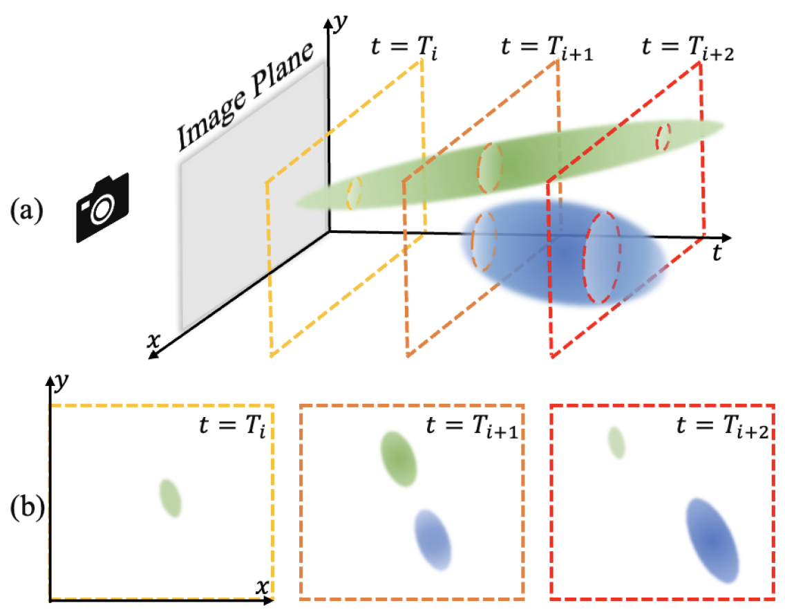
我们的主要观察结果是，每个时间戳的 3D 场景动态可以被视为使用不同时间查询切片的 4D 时空高斯椭球体。图2说明了一个简化的 $X Y T$ 情况：2D $X Y$ 空间在时间 $T_{i}$ 的动态相当于构建3D $X Y T$ 高斯分布和 $t=T_{i}$ 平面切片。类似地，我们将 3D 高斯扩展到 4D $X Y Z T$ 空间来建模动态 3D 场景。时间切片的4D高斯组成3D高斯，可以通过快速光栅化无缝投影到2D屏幕，继承了3DGS的精致渲染效果和高速特性。此外，在时间维度上扩展剪枝分裂机制使得 4D 高斯特别适合表示复杂的动态，包括突然出现或消失。

将 3D 高斯模型提升到 4D 空间并非易事，其中 4D 旋转、切片以及联合时空优化方案的设计存在巨大挑战。我们从几何代数中汲取灵感，精心选择4D转子[6]来表示4D旋转，这是一种时空可分离的旋转表示。值得注意的是，转子表示同时支持 3D 和 4D 旋转：当时间维度设置为零时，它相当于四元数，并且也可以表示 3D 空间旋转。这种适应性使我们的方法能够灵活地对动态和静态场景进行建模。换句话说，4DGS 是 3DGS 的概括形式：当关闭时间维度时，我们的 4DGS 简化为 3DGS。

我们增强了 3DGS 中的优化策略，并引入了两个新的正则化项来稳定和改进动态重建。我们首先提出一种熵损失，将高斯的不透明度推向 1 或 0，这在我们的实验中证明可以有效去除“漂浮物”。我们进一步引入了一种新颖的 4D 一致性损失来规范高斯点的运动并产生更一致的动态重建。实验表明，这两项都显着提高了渲染质量。

虽然现有的基于高斯的方法[35,60,56,61]大多基于PyTorch[41]，但我们通过仔细的工程设计进一步开发了高度优化的CUDA框架用于快速训练和推理速度。我们的框架支持在 RTX 4090 GPU 上以前所未有的 583 FPS 渲染 1352 $\times$ 1014 个视频，在 RTX 3090 GPU 上以前所未有的 277 FPS 渲染。我们对涵盖各种设置和运动模式的两个数据集进行了广泛的实验，包括单目视频 [43] 和多摄像头视频 [33]。定量和定性评估证明了与先前方法相比的明显优势，包括新的最先进的渲染质量和速度。

2相关工作

Refer to caption — 图2：拟议时间切片的简化 2D 插图。 (a) 我们使用 3D $X Y T$ 椭球体对 2D 动力学进行建模，并使用不同的时间查询对它们进行切片。 (b) 切片 3D 椭球在每个时间戳处形成 2D 动态椭圆。

在本节中，我们主要回顾基于优化的新颖视图合成（NVS）方法，其中输入是一组姿势图像，输出是来自新颖视点的新外观。我们首先描述静态场景的NVS，然后讨论它的动态扩展。最后，我们讨论最近基于高斯的 NVS 方法。

静态新颖视图合成先前的方法将光场 [30] 或 Lumigraph [22, 7] 形式化，通过插值生成新颖视图图像现有的视图需要密集捕获的图像才能获得逼真的渲染。其他经典方法利用网格和体积等几何代理将源图像中的内容重新投影和混合到新颖的视图上。基于网格的方法[13,44,49,53,55]表示具有支持高效渲染但难以优化的表面的场景。基于体积的方法使用体素网格 [29, 42, 45] 或多平面图像 (MPI) [17, 36, 48, 63]，提供精致的渲染效果，但内存效率低下或仅限于较小的视图更改。最近，神经辐射场 (NeRFs) [37] 引领了 NVS 的趋势，它实现了照片级真实感的渲染质量。此后，出现了一系列的努力，以提高训练速度[38, 18, 10]，增强渲染质量[3, 52]，或扩展到更具挑战性反射和折射等场景[28,5,59]。尽管如此，这些方法大多数依赖于体积渲染，需要对数百万条光线进行采样并阻碍实时渲染[37,3,10]。

动态小说视图合成由于输入图像的时间变化，这提出了新的挑战。传统方法会估计不同的几何形状，例如表面 [31, 12] 和深度图 [25, 64]，以考虑动态。受 NeRF 的启发，最近的工作通常使用神经表示来建模动态场景。方法的一个分支通过添加时间输入或潜在代码 [14, 21] 来隐式建模动态。另一系列作品[39,40,51,43,15]显式地对变形场进行建模，将任意时间戳处的 3D 点映射到规范空间中。其他技术探索将场景分解为静态和动态组件[47]，使用关键帧减少冗余[33, 2]，估计流场[34 , 23, 50]，或利用基于 4D 网格的表示[32, 19, 8, 54, 15, 20, 46],等。动态场景建模的常见问题是时空纠缠带来的复杂性，以及时间维度带来的额外内存和时间成本。

基于高斯的 NVS 最近的开创性工作[62, 58, 1, 26] 使用高斯对静态场景进行建模，其位置和外观是通过可微分的基于泼溅的渲染器学习的。特别是，3D 高斯泼溅 (3DGS)[26] 凭借其高斯分割/克隆操作和基于快速泼溅的渲染技术，实现了令人印象深刻的实时渲染。我们的工作从 3DGS 中汲取灵感，但将 3D 高斯模型提升到 4D 空间，并专注于动态场景。几项并行工作还将 3DGS 扩展到动力学模型。 Deformable3DGS [35] 直接学习每个 3D 高斯随时间的时间运动和旋转，这使得它适合动态跟踪应用。类似地，[60, 56]利用 MLP 来预测时间运动。然而，这些方法很难表示突然出现或消失的动态内容。与我们类似，RealTime4DGS [61] 也利用 4D 高斯表示来建模 3D 动力学。他们选择了基于双四元数的 4D 旋转公式，与基于转子的表示相比，该公式的可解释性较差，并且缺乏时空可分离属性。此外，我们进一步研究更好的时空优化策略，并开发一个高性能框架，以实现更高的渲染速度和更好的渲染质量。

3方法

在本节中，我们首先回顾第 2 节中的 3D 高斯分布 (3DGS) 方法[26]。 3.1。然后我们在第 2 节中描述我们的 4G 高斯分布算法。 3.2，我们在第 2 节中介绍了基于转子的 4D 高斯表示。 3.2.1 并在第 3 节中讨论可微分实时光栅化的时间切片技术。 3.2.2。最后，我们在第二节介绍了我们的动态优化策略。 3.3。

3.1 3D高斯泼溅初步

3D 高斯泼溅 (3DGS) [26] 已在静态场景上展示了最先进的实时渲染质量。它对具有密集 $N$ 各向异性 3D 高斯椭球簇的场景进行建模。每个高斯由完整的 3D 协方差矩阵 $\mathbf{\Sigma}$ 及其中心位置 $\mathbf{\mu}$ 表示：

{G}(\mathbf{x})=e^{-\frac{1}{2}(\mathbf{x}-\mathbf{\mu})^{T}\mathbf{\Sigma}^{-1}(\mathbf{x}-\mathbf{\mu})}.

(1)

为了确保优化期间有效的正半定协方差矩阵， $\mathbf{\Sigma}$ 被分解为缩放矩阵 $\mathbf{S}$ 和旋转矩阵 $\mathbf{R}$ 来表征a的几何形状3D 高斯椭球：

\mathbf{\Sigma}=\mathbf{R}\mathbf{S}\mathbf{S}^{T}\mathbf{R}^{T},

(2)

其中 $\mathbf{S}=\text{diag}(s_{x},s_{y},s_{z})\in\mathbb{R}^{3}$ 和 $\mathbf{R}\in SO(3)$ 分别存储为 $3D$ 向量和四元数。除了 $\mathbf{\mu}$ 、 $\mathbf{S}$ 和 $\mathbf{R}$ ，每个高斯还保留了其他可学习的参数，包括不透明度 $o\in(0,1)$ 和 $\mathbb{R}^{k}$ 中代表视角相关颜色的球谐波 (SH) 系数（ $k$ 与 SH 阶数有关）。在优化过程中，3DGS 通过在具有大视空间位置梯度的区域中分割和克隆高斯分布以及剔除表现出接近透明的高斯分布来自适应控制高斯分布。

3DGS 中的高效渲染和参数优化由基于可微图块的光栅化器提供支持。首先，通过计算相机空间协方差矩阵 $\mathbf{\Sigma^{\prime}}$ 将3D高斯投影到2D空间：

\mathbf{\Sigma^{\prime}}=\mathbf{J}\mathbf{V}\mathbf{\Sigma}\mathbf{V}^{T}\mathbf{J}^{T},

(3)

其中 $\mathbf{J}$ 是投影变换的仿射近似的雅可比矩阵， $\mathbf{V}$ 是外在相机矩阵。然后，通过混合按深度排序的高斯来计算图像平面上每个像素的颜色：

C=\sum_{i=1}^{N}c_{i}\alpha_{i}\prod_{j=1}^{i-1}(1-\alpha_{j}),

(4)

其中 $c_{i}$ 是第 $i$ 个 3D 高斯 ${G}_{i}$ 、 $\alpha_{i}=o_{i}G^{\prime}_{i}$ 以及 $o_{i}$ 和 $G^{\prime}_{i}$ 分别作为 ${G}_{i}$ 的不透明度和 2D 投影。请参阅 3DGS [26] 了解更多详细信息。

3.2 4D 高斯分布

我们现在讨论 4D 高斯分布 (4DGS) 算法。具体来说，我们使用基于转子的旋转表示对 4D 高斯进行建模（第 3.2.1 节），并对时间维度进行切片以在每个时间戳生成动态 3D 高斯（第 3.2.2)。在每个时间戳处切片的 3D 高斯椭球体可以有效地光栅化到 2D 图像平面上，以实现动态场景的实时高保真渲染。

3.2.1 基于转子的4D高斯表示

与 3D 高斯类似，4D 高斯可以用 4D 中心位置 $\mathbf{\mu}_{4D}=(\mathbf{\mu}_{x},\mathbf{\mu}_{y},\mathbf{\mu}_{z},\mathbf{\mu}_{t})$ 和 4D 协方差矩阵 $\mathbf{\Sigma}_{4D}$ 表示为

{G}_{4D}(x)=e^{-\frac{1}{2}(x-\mathbf{\mu}_{4D})^{T}\mathbf{\Sigma}_{4D}^{-1}(x-\mathbf{\mu}_{4D})}.

(5)

协方差 $\Sigma_{4D}$ 可以进一步分解为4D缩放 $S_{4D}$ 和4D旋转 $R_{4D}$ 为

\mathbf{\Sigma}_{4D}=\mathbf{R}_{4D}\mathbf{S}_{4D}\mathbf{S}_{4D}^{T}\mathbf{R}_{4D}^{T}.

(6)

虽然建模 $\mathbf{S}_{4D}=\text{diag}(s_{x},s_{y},s_{z},s_{t})$ 很简单，但为 $R_{4D}$ 寻找合适的 4D 旋转表示是一个具有挑战性的问题。

在几何代数中，高维向量的旋转可以使用转子[6]来描述。受此启发，我们引入 4D 转子来表征 4D 旋转。 4D 转子 $\mathbf{r}$ 由 8 个基于一组基础的组件组成：

	$\displaystyle\mathbf{r}$	$\displaystyle=s+b_{01}\mathbf{e}_{01}+b_{02}\mathbf{e}_{02}+b_{03}\mathbf{e}_{03}+b_{12}\mathbf{e}_{12}$
		$\displaystyle\quad+b_{13}\mathbf{e}_{13}+b_{23}\mathbf{e}_{23}+p\mathbf{e}_{0123},$		(7)

其中 $\mathbf{e}_{0123}=\mathbf{e}_{0}\wedge\mathbf{e}_{1}\wedge\mathbf{e}_{2}\wedge\mathbf{e}_{3}$ 和 $\mathbf{e}_{ij}=\mathbf{e}_{i}\wedge\mathbf{e}_{j}$ 是 4D 轴 $\mathbf{e}_{i}$ ( $i\in\{0,1,2,3\}$ ) 之间的外积，它们构成 4D 欧几里德空间中的正交基。因此，可以通过8个系数 $\left(s,b_{01},b_{02},b_{03},b_{12},b_{13},b_{23},p\right)$ 来确定4D旋转。

与四元数类似，转子 $\mathbf{r}$ 也可以通过适当的归一化函数 $\mathcal{F}_{norm}$ 和转子矩阵映射函数 $\mathcal{F}_{map}$ 转换为四维旋转矩阵 $\mathbf{R}_{4D}$ 。我们仔细推导了一种用于转子变换的数值稳定归一化方法，并在补充材料中提供了两个函数的详细信息：

\mathbf{R}_{4D}=\mathcal{F}_{map}(\mathcal{F}_{norm}(\mathbf{r})).

(8)

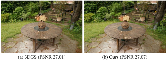
我们基于转子的 4D 高斯提供了定义明确、可解释的旋转表示：前四个分量编码 3D 空间旋转，后四个分量定义时空旋转，即。，空间平移。特别是，将最后四个分量设置为零可以有效地将 $\mathbf{r}$ 减少为 3D 空间旋转的四元数，从而使我们的框架能够对静态和动态场景进行建模。图 4 展示了一个示例，其中我们在静态 3D 场景上的结果与原始 3DGS [26] 的结果相匹配。

另外，并发工作[61]还使用 4D 高斯对动态场景进行建模。然而，它们表示具有两个纠缠等斜四元数 [9] 的 4D 旋转。因此，它们的空间和时间旋转紧密耦合，并且尚不清楚如何在静态 3D 场景建模优化过程中约束和规范化这种替代旋转表示。

3.2.2 时间切片 4D 高斯泼溅

我们现在描述如何将 4D 高斯分割成 3D 空间。鉴于 $\mathbf{\Sigma}_{4D}$ 及其逆 $\mathbf{\Sigma}_{4D}^{-1}$ 都是对称矩阵，我们定义

\mathbf{\Sigma}_{4D}=\left(\begin{matrix}\mathbf{U}&\mathbf{V}\\ \mathbf{V}^{T}&\mathbf{W}\\ \end{matrix}\right)\text{~{}and~{}}\mathbf{\Sigma}_{4D}^{-1}=\left(\begin{matrix}\mathbf{A}&\mathbf{M}\\ \mathbf{M}^{T}&\mathbf{Z}\\ \end{matrix}\right),

(9)

其中 $\mathbf{U}$ 和 $\mathbf{A}$ 都是 $3\times 3$ 矩阵。然后，给定时间 $t$ ，投影 3D 高斯分布如下（补充材料中的详细推导）：

{G}_{3D}(\mathbf{x},t)=\text{e}^{-\frac{1}{2}\lambda(t-\mathbf{\mu}_{t})^{2}}\text{e}^{-\frac{1}{2}\left[\mathbf{x}-\mathbf{\mu}(t)\right]^{T}\mathbf{\Sigma}_{3D}^{-1}\left[\mathbf{x}-\mathbf{\mu}(t)\right]},

(10)

在哪里

$\displaystyle\lambda$	$\displaystyle=\mathbf{W}^{-1},$	(11)
$\displaystyle\mathbf{\Sigma}_{3D}$	$\displaystyle=\mathbf{A}^{-1}=\mathbf{U}-\dfrac{\mathbf{V}\mathbf{V}^{T}}{\mathbf{W}},$
$\displaystyle\mathbf{\mu}(t)$	$\displaystyle=(\mathbf{\mu}_{x},\mathbf{\mu}_{y},\mathbf{\mu}_{z})^{T}+(t-\mathbf{\mu}_{t})\dfrac{\mathbf{V}}{\mathbf{W}}.$

与等式相比原始 3DGS [26] 中的 1，等式中的切片 3D 高斯。 10 包含时间衰减项 $\text{e}^{-\frac{1}{2}\lambda(t-\mathbf{\mu}_{t})^{2}}$ 。随着 $t$ 的流逝，一旦 $t$ 足够接近其时间位置 $\mathbf{\mu}_{t}$ 并开始增长，高斯点首先出现。当 $t=\mathbf{\mu}_{t}$ 时，其达到不透明度峰值。之后，3D 高斯的密度逐渐缩小，直到 $t$ 距离 $\mathbf{\mu}_{t}$ 足够远时消失。通过控制时间位置和缩放因子，4D 高斯可以表示具有挑战性的动态，例如.，突然出现或消失的运动。在渲染过程中，我们过滤掉距离当前时间太远的点，其中可见性阈值 $\frac{1}{2}\lambda(t-\mathbf{\mu}_{t})^{2}$ 根据经验设置为16。

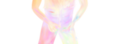
此外，切片 3D 高斯呈现出添加到中心位置 $(\mathbf{\mu}_{x},\mathbf{\mu}_{y},\mathbf{\mu}_{z})^{T}$ 的新运动项 $(t-\mathbf{\mu}_{t}){\mathbf{V}}/{\mathbf{W}}$ 。理论上，3D 高斯的线性运动是从我们的 4D 切片操作中产生的。我们假设在很小的时间间隔内，所有运动都可以用线性运动来近似，更复杂的非线性情况可以用多个高斯的组合来表示。进一步地， ${\mathbf{V}}/{\mathbf{W}}$ 表示当前时间戳下的运动速度。因此，通过使用我们的框架对场景进行建模，我们可以免费获取速度场。我们在图 8 中可视化光流。

最后，按照3DGS [26]，我们将切片的3D高斯按深度顺序投影到2D图像平面，并执行快速可微光栅化以获得最终图像。我们在高性能 CUDA 框架中实现了转子表示和切片，并且与 PyTorch 实现相比实现了更高的渲染速度。

3.3优化架构

当将 3D 高斯提升到 4D 空间时，增加的维度扩展了高斯点的自由度。因此，我们引入两个正则化术语来帮助稳定训练过程：熵损失和4D一致性损失。

3.3.1 熵损失

与NeRF类似，每个高斯点都有一个可学习的不透明度项 $o_{i}$ ，并应用体积渲染公式来合成最终颜色。理想情况下，高斯点应靠近物体表面，并且在大多数情况下其不透明度应接近 1。因此，我们通过添加熵损失来鼓励不透明度接近 1 或接近于 0，并且默认情况下，不透明度接近于零的高斯将在期间被修剪：

\displaystyle L_{\text{entropy}}=

\displaystyle\frac{1}{N}\sum_{i=1}^{N}-o_{i}log(o_{i}).

(12)

我们发现 $L_{\text{entropy}}$ 有助于压缩高斯点并过滤嘈杂的漂浮物，这在使用稀疏视图进行训练时非常有用。

3.3.2 4D一致性损失

直观上，4D 空间中附近的高斯应该有类似的运动。我们通过添加 4D 时空一致性损失来进一步规范 4D 高斯点。回想一下，在给定时间 $t$ 对 4D 高斯进行切片时，会导出速度项 $\mathbf{s}$ 。因此，给定第 $i$ 个高斯点，我们从其相邻空间 $\Omega_{i}$ 收集 $K$ 个最近的 4D 点，并将它们的运动正则化以保持一致：

\displaystyle L_{\text{consistent4D}}=

\displaystyle\frac{1}{N}\sum_{i=1}^{N}\left|\left|\mathbf{s}_{i}-\frac{1}{K}\sum_{j\in\Omega_{i}}\mathbf{s}_{j}\right|\right|_{1}.

(13)

对于 4D 高斯，4D 距离是比 3D 距离更好的点相似性度量，因为 3D 中相邻的点不一定遵循相同的运动，例如。，当它们属于具有不同运动的两个物体。请注意，计算 4D 最近邻在我们的 4D 表示中是唯一且自然地启用的，基于变形的方法无法利用它[56]。我们通过除以相应的空间和时间场景尺度来平衡每个维度的不同尺度。

3.3.3 总损失

我们遵循原始 3DGS [26] 并在渲染图像和地面实况图像之间添加 $L_{1}$ 和 SSIM 损失。我们最终的损失定义为：

\displaystyle L=

\displaystyle(1-\lambda_{1})L_{1}+\lambda_{1}L_{ssim}+\lambda_{2}L_{\text{entropy}}+\lambda_{3}L_{\text{consistent4D}}.

(14)

3.3.4优化框架

我们实现了方法的两个版本：一种使用 PyTorch 进行快速开发，另一种使用 C++ 和 CUDA 进行高度优化，用于快速训练和推理。与 PyTorch 版本相比，我们的 CUDA 加速允许在单个 NVIDIA RTX 4090 GPU 上以前所未有的 583 FPS、1352 $\times$ 1014 分辨率进行渲染。此外，我们的 CUDA 框架还将训练速度提高了 16.6 倍。为了进行基准测试，我们还在 RTX 3090 GPU 上测试了我们的框架，并达到了 277 FPS，这明显优于当前的技术水平（114 FPS [61])。

4实验

4.1数据集

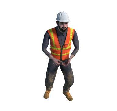
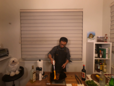
我们在两个常用的数据集上评估我们的方法，这两个数据集代表了动态场景建模中的各种挑战。 Plenoptic 视频数据集 [33] 包含 6 个场景的真实多视图视频。它包括突然的运动以及透明和反光材料。根据之前的工作[33]，我们使用分辨率 1352 $\times$ 1014。 D-NeRF 数据集 [43] 包含 8 个合成场景的一秒单目视频。我们按照标准做法 [43] 使用 400 $\times$ 400 的分辨率。

4.2实现细节

初始化。我们在 4D 边界框中均匀采样 100,000 个点作为高斯均值。对于 Plenoptic 数据集，我们使用彩色 COLMAP [16] 重建进行初始化。 3D 比例设置为到最近邻居的距离。转子使用相当于静态恒等变换的 $(1,0,0,0,0,0,0,0)$ 进行初始化。

训练。使用 Adam 优化器，我们在 D-NeRF 数据集上训练批量大小为 3 的 20,000 个步骤，在 Plenoptic 数据集上训练批量大小为 2 的 30,000 个步骤。 D-NeRF 和 Plenoptic 数据集的致密梯度阈值分别为 $5e-5$ 和 $2e-4$ 。我们设置 $\lambda_{1}=0.2,\lambda_{2}=0.01,\lambda_{3}=0.05$ 和 $K=8$ ，但Plenoptic数据集的 $\lambda_{2}=0$ 除外，因为它的视频包含大量透明物体。学习率、致密化、修剪和不透明度重置设置均遵循[26]。

CUDA 加速。我们在定制的 CUDA 训练框架中实现了 4D 转子的前向和后向函数到 4D 旋转矩阵和 4D 高斯切片。 4D 高斯的复制和修剪也由 CUDA 执行，确保较低的 GPU 内存使用量。

4.3基线

我们在两个数据集上比较了基于 NeRF 和并发高斯的方法。大多数比较方法都已发布官方代码库，在这种情况下，我们按原样运行代码并报告获得的新视图渲染质量、训练时间和推理速度的数据。否则，我们会复制他们论文中的结果。表中报告的所有数字均以 NVIDIA RTX 3090 GPU 为基准。

4.4结果

4.4.1 Plenoptic视频数据集评估

如选项卡中详细说明。 1，由于体渲染速度慢(a-f)、时间成本，之前的工作在渲染速度和质量之间进行权衡查询神经网络组件(c、d、g)或时空纠缠(a、 c,g)。然而，我们的方法表现出显着的优势。最重要的是，它在 NVIDIA RTX 3090 GPU 上以 277 FPS 渲染高分辨率视频 (1352 $\times$ 1014) 方面的性能明显优于现有工作，比基于 NeRF 的方法快 10 倍以上 (a) >-f)，比基于高斯的方法(g、h)快 2 倍以上。此外，我们的方法实现了 31.62 的最高 PSNR(vs. 之前的最佳值 30.85），平均训练时间很短，为 60 分钟。

如图5所示，我们的方法促进了基线上动态区域的更清晰、更详细的重建。对于所有四个场景，所提出的方法重建了频繁移动并包含高频细节的更高质量的人体头部。正如前三个场景中放大的那样，基线可能会为快速运动的手部区域产生模糊的伪影。相比之下，我们的方法对相同区域产生最清晰的渲染。

表1：全光视频数据集评估. 我们将我们的方法与基于 NeRF 和基于高斯的方法进行比较。我们的方法在 PSNR 和推理速度方面显着优于基线。 *：仅在场景火焰鲑鱼上进行测试。 **：在 8 个 GPU 上进行训练。 †：论文结果。

ID	Method	PSNR $\uparrow$	SSIM $\uparrow$	LPIPS $\downarrow$	Train $\downarrow$	FPS $\uparrow$
a	DyNeRF [33]*†	29.58	-	0.08	1344 h**	0.015
b	StreamRF [32]	28.16	0.85	0.31	79 min	8.50
c	HyperReel [2]	30.36	0.92	0.17	9 h	2.00
d	NeRFPlayer [47]†	30.69	-	0.11	6 h	0.05
e	K-Planes [19]	30.73	0.93	0.07	190 min	0.10
f	MixVoxels [54]	30.85	0.96	0.21	91 min	16.70
g	Deformable4DGS [56]	28.42	0.92	0.17	72 min	39.93
h	RealTime4DGS [61]	29.95	0.92	0.16	8 h	72.80
i	Ours	31.62	0.94	0.14	60 min	277.47

	Lego	Jumping Jacks	Stand Up	T-Rex	Hook
TiNeuVox
Deformable4DGS
RealTime4DGS
Ours
Ground Truth

图6：我们的方法和 D-NeRF 数据集基线的定性比较。我们与基于 NeRF (TiNeuVox [15]) 和基于 Gaussian (Deformable4DGS [56] 和 RealTime4DGS [61]) 的方法进行比较。正如突出显示的区域所示，我们的方法能够以更少的噪音和更多的细节重建场景，例如。,乐高的刀片推土机、Jumping Jacks和Hook中的袖口和手、T-Rex中的牙齿以及中的头盔和面部细节站起来。

4.4.2 D-NeRF数据集评估

由于输入视图稀疏，单目视频 NVS 特别具有挑战性。正如表中所总结的。 2、[60] 实现了最高的 PSNR，因为它直接跟踪 3D 高斯点的变形，与 D-NeRF 数据集完美对齐。除此之外，我们的方法在所有其他方法中实现了最佳渲染质量，渲染速度为 1258 FPS（比之前的最佳速度快 8 倍）。此外，在我们的快速实施中，训练只需要大约 5 分钟。

图6展示了这项工作如何在减少飞蚊症和增强重建方面超越基线。例如，乐高推土机的刀片现在更加明确。在Jumping Jacks中，我们的方法生成形状更清晰的手指，并消除了基线结果中观察到的伪影，例如。，行中袖口旁边的漂浮物3. 在Stand Up中，头盔和面部特征上的图案在我们的结果中更加明显。基线结果中缺失的牙齿细节在我们的结果中得到了恢复。此外，所提出的方法还减轻了Hook手上的噪音，从而使手指更加清晰。

	Lego	Hook	T-Rex	Hell Warrior	Bouncing Balls
Original Setting
+ Entropy Loss
+ KNN Loss
+ Batch Training
Ground Truth

图7： D-NeRF数据集的消融研究。每行都将不同的组件（左）添加到其上方行的设置中。比较前两行的场景，我们可以看到熵损失有助于减少飞蚊症。此外，KNN损失和Batch训练都有助于锐化外观细节，例如.,Hook的手和T的头部-Rex，以及重建更好的几何形状，例如。,乐高的刀片，地狱的脚战士，以及弹跳球的形状。

4.5消融研究

标签。 3 削弱了我们的方法在具有挑战性的 D-NeRF 数据集上的各个设计的有效性。

熵损失。如表所示。 3 (b)，添加熵损失可显着减少点数大约 1，同时保持 PSNR 和 SSIM 中测量的整体渲染质量。图7清楚地揭示了熵损失的影响。例如，第 1 行中场景周围的漂浮物 Lego、Hook 和 Bouncing Balls 已在第 2 行中完全移除。这表明熵损失有助于在优化过程中对 4D 高斯点分布施加强约束。然而，我们还发现它会导致 Plenoptic 数据集中的 PSNR 下降。我们认为这是因为 Plenoptic 数据集提供了密集的视图并包含大量透明对象。因此，我们建议为不透明表面和稀疏视图添加熵损失。

4D 一致性损失。本来，4D空间中相邻高斯的状态可以自由变化，这增加了优化的难度和模型的冗余。然而，4D 一致性损失的应用增强了空间和时间维度上的局部一致性。这在图7，选项卡中得到证实。 3 (c) 和图 8，其中 4D 一致性损失有助于恢复一致的运动、添加更多细节并提高渲染质量。

批量训练。批量训练有助于减少梯度噪声并稳定训练。标签。 3 (Full) 显示批处理训练比设置 (c) 进一步提高了渲染质量。对于单目视频等稀疏视图设置，批量训练还可以通过在多个视图上联合优化来帮助提高几何一致性，如图7、例如所示。，脚在地狱战士。

5结论

在这项工作中，我们提出了 4D 高斯泼溅，这是一种能够实现高质量 4D 动态场景建模的新颖方法。我们的方法大幅优于现有技术，并在 RTX 4090 GPU 上实现了前所未有的 583 FPS 渲染速度。此外，这是一个用于 3D 静态和 4D 动态重建的统一框架。我们会将代码发布到社区，以方便相关研究。

虽然我们已经实现了最先进的重建质量，但我们观察到，由于维度增加，4D 高斯很难约束并导致诸如飞蚊症和不一致运动之类的伪影。虽然熵损失和 4D 一致性损失有助于缓解这些问题，但伪影仍然存在。未来的方向包括利用 4D 高斯函数进行下游任务，例如跟踪和动态场景生成。

表2： D-NeRF数据集评估. 我们与最近基于 NeRF 和基于 Gaussian 的方法进行比较。我们的方法在 PSNR 和渲染速度方面都远远优于基线。

Method	PSNR $\uparrow$	SSIM $\uparrow$	LPIPS $\downarrow$	Train $\downarrow$	FPS $\uparrow$
D-NeRF [43]	29.17	0.95	0.07	24 h	0.13
TiNeuVox [15]	32.87	0.97	0.04	28 min	1.60
K-Planes [19]	31.07	0.97	0.02	54 min	1.20
Deformable3DGS [60]	39.31	0.99	0.01	26 min	85.45
Deformable4DGS [56]	32.99	0.97	0.05	13 min	104.00
RealTime4DGS [61]	32.71	0.97	0.03	10 min	289.07
Ours	34.26	0.97	0.03	5 min	1257.63

表3： D-NeRF 数据集上的 4DGS 消融. 我们验证了渲染质量和点数（以百万为单位）的三种设计：(b) 熵（具有交叉熵损失）、(c) KNN（具有 4D KNN一致性损失）和(Full)批量（带有批量训练）。

ID				D-NeRF
	Entropy	KNN	Batch	PSNR $\uparrow$	SSIM $\uparrow$	#Point(M) $\downarrow$
a				31.53	0.96	$1.7e5$
b	✓			31.50	0.97	$5.4e4$
c	✓	✓		31.91	0.97	$3.0e5$
Full	✓	✓	✓	33.06	0.98	$1.4e5$

参考

Abou-Chakra et al. [2022] Jad Abou-Chakra, Feras Dayoub, and Niko Sünderhauf. Particlenerf: Particle based encoding for online neural radiance fields in dynamic scenes. arXiv preprint arXiv:2211.04041, 2022.
Attal et al. [2023] Benjamin Attal, Jia-Bin Huang, Christian Richardt, Michael Zollhoefer, Johannes Kopf, Matthew O’Toole, and Changil Kim. Hyperreel: High-fidelity 6-dof video with ray-conditioned sampling. In Proceedings of the IEEE/CVF Conference on Computer Vision and Pattern Recognition, pages 16610–16620, 2023.
Barron et al. [2021] Jonathan T Barron, Ben Mildenhall, Matthew Tancik, Peter Hedman, Ricardo Martin-Brualla, and Pratul P Srinivasan. Mip-nerf: A multiscale representation for anti-aliasing neural radiance fields. In Proceedings of the IEEE/CVF International Conference on Computer Vision, pages 5855–5864, 2021.
Barron et al. [2022] Jonathan T Barron, Ben Mildenhall, Dor Verbin, Pratul P Srinivasan, and Peter Hedman. Mip-nerf 360: Unbounded anti-aliased neural radiance fields. In Proceedings of the IEEE/CVF Conference on Computer Vision and Pattern Recognition, pages 5470–5479, 2022.
Bemana et al. [2022] Mojtaba Bemana, Karol Myszkowski, Jeppe Revall Frisvad, Hans-Peter Seidel, and Tobias Ritschel. Eikonal fields for refractive novel-view synthesis. In ACM SIGGRAPH 2022 Conference Proceedings, pages 1–9, 2022.
Bosch [2020] Marc Ten Bosch. N-dimensional rigid body dynamics. ACM Transactions on Graphics (TOG), 39(4):55–1, 2020.
Buehler et al. [2001] Chris Buehler, Michael Bosse, Leonard McMillan, Steven Gortler, and Michael Cohen. Unstructured lumigraph rendering. ACM Transactions on Graphics (Proc. SIGGRAPH), 2001.
Cao and Johnson [2023] Ang Cao and Justin Johnson. Hexplane: A fast representation for dynamic scenes. In Proceedings of the IEEE/CVF Conference on Computer Vision and Pattern Recognition, pages 130–141, 2023.
Cayley [1894] Arthur Cayley. The collected mathematical papers of Arthur Cayley. University of Michigan Library, 1894.
Chen et al. [2022] Anpei Chen, Zexiang Xu, Andreas Geiger, Jingyi Yu, and Hao Su. Tensorf: Tensorial radiance fields. In European Conference on Computer Vision, pages 333–350. Springer, 2022.
Cheng et al. [2023] Wei Cheng, Ruixiang Chen, Siming Fan, Wanqi Yin, Keyu Chen, Zhongang Cai, Jingbo Wang, Yang Gao, Zhengming Yu, Zhengyu Lin, et al. Dna-rendering: A diverse neural actor repository for high-fidelity human-centric rendering. In Proceedings of the IEEE/CVF International Conference on Computer Vision, pages 19982–19993, 2023.
Collet et al. [2015] Alvaro Collet, Ming Chuang, Pat Sweeney, Don Gillett, Dennis Evseev, David Calabrese, Hugues Hoppe, Adam Kirk, and Steve Sullivan. High-quality streamable free-viewpoint video. ACM Transactions on Graphics (ToG), 34(4):1–13, 2015.
Debevec et al. [1996] Paul E Debevec, Camillo J Taylor, and Jitendra Malik. Modeling and rendering architecture from photographs: A hybrid geometry-and image-based approach. ACM Transactions on Graphics (Proc. SIGGRAPH), 1996.
Du et al. [2021] Yilun Du, Yinan Zhang, Hong-Xing Yu, Joshua B Tenenbaum, and Jiajun Wu. Neural radiance flow for 4d view synthesis and video processing. In 2021 IEEE/CVF International Conference on Computer Vision (ICCV), pages 14304–14314. IEEE Computer Society, 2021.
Fang et al. [2022] Jiemin Fang, Taoran Yi, Xinggang Wang, Lingxi Xie, Xiaopeng Zhang, Wenyu Liu, Matthias Nießner, and Qi Tian. Fast dynamic radiance fields with time-aware neural voxels. In SIGGRAPH Asia 2022 Conference Papers, pages 1–9, 2022.
Fisher et al. [2021] Alex Fisher, Ricardo Cannizzaro, Madeleine Cochrane, Chatura Nagahawatte, and Jennifer L Palmer. Colmap: A memory-efficient occupancy grid mapping framework. Robotics and Autonomous Systems, 142:103755, 2021.
Flynn et al. [2019] John Flynn, Michael Broxton, Paul Debevec, Matthew DuVall, Graham Fyffe, Ryan Overbeck, Noah Snavely, and Richard Tucker. Deepview: View synthesis with learned gradient descent. In Proceedings of the IEEE/CVF Conference on Computer Vision and Pattern Recognition, pages 2367–2376, 2019.
Fridovich-Keil et al. [2022] Sara Fridovich-Keil, Alex Yu, Matthew Tancik, Qinhong Chen, Benjamin Recht, and Angjoo Kanazawa. Plenoxels: Radiance fields without neural networks. In Proceedings of the IEEE/CVF Conference on Computer Vision and Pattern Recognition, pages 5501–5510, 2022.
Fridovich-Keil et al. [2023] Sara Fridovich-Keil, Giacomo Meanti, Frederik Rahbæk Warburg, Benjamin Recht, and Angjoo Kanazawa. K-planes: Explicit radiance fields in space, time, and appearance. In Proceedings of the IEEE/CVF Conference on Computer Vision and Pattern Recognition, pages 12479–12488, 2023.
Gan et al. [2023] Wanshui Gan, Hongbin Xu, Yi Huang, Shifeng Chen, and Naoto Yokoya. V4d: Voxel for 4d novel view synthesis. IEEE Transactions on Visualization and Computer Graphics, 2023.
Gao et al. [2021] Chen Gao, Ayush Saraf, Johannes Kopf, and Jia-Bin Huang. Dynamic view synthesis from dynamic monocular video. In Proceedings of the IEEE/CVF International Conference on Computer Vision, pages 5712–5721, 2021.
Gortler et al. [1996] Steven J. Gortler, Radek Grzeszczuk, Richard Szeliski, and Michael F. Cohen. Light field rendering. ACM Transactions on Graphics (Proc. SIGGRAPH), 1996.
Guo et al. [2023] Xiang Guo, Jiadai Sun, Yuchao Dai, Guanying Chen, Xiaoqing Ye, Xiao Tan, Errui Ding, Yumeng Zhang, and Jingdong Wang. Forward flow for novel view synthesis of dynamic scenes. In Proceedings of the IEEE/CVF International Conference on Computer Vision, pages 16022–16033, 2023.
Hedman et al. [2018] Peter Hedman, Julien Philip, True Price, Jan-Michael Frahm, George Drettakis, and Gabriel Brostow. Deep blending for free-viewpoint image-based rendering. ACM Transactions on Graphics (ToG), 37(6):1–15, 2018.
Kanade et al. [1997] Takeo Kanade, Peter Rander, and PJ Narayanan. Virtualized reality: Constructing virtual worlds from real scenes. IEEE multimedia, 4(1):34–47, 1997.
Kerbl et al. [2023] Bernhard Kerbl, Georgios Kopanas, Thomas Leimkühler, and George Drettakis. 3d gaussian splatting for real-time radiance field rendering. ACM Transactions on Graphics (ToG), 42(4):1–14, 2023.
Knapitsch et al. [2017] Arno Knapitsch, Jaesik Park, Qian-Yi Zhou, and Vladlen Koltun. Tanks and temples: Benchmarking large-scale scene reconstruction. ACM Transactions on Graphics (ToG), 36(4):1–13, 2017.
Kopanas et al. [2022] Georgios Kopanas, Thomas Leimkühler, Gilles Rainer, Clément Jambon, and George Drettakis. Neural point catacaustics for novel-view synthesis of reflections. ACM Transactions on Graphics (TOG), 41(6):1–15, 2022.
Kutulakos and Seitz [2000] Kiriakos N Kutulakos and Steven M Seitz. A theory of shape by space carving. International journal of computer vision, 38:199–218, 2000.
Levoy and Hanrahan [1996] Marc Levoy and Pat Hanrahan. Light field rendering. ACM Transactions on Graphics (Proc. SIGGRAPH), 1996.
Li et al. [2012] Hao Li, Linjie Luo, Daniel Vlasic, Pieter Peers, Jovan Popović, Mark Pauly, and Szymon Rusinkiewicz. Temporally coherent completion of dynamic shapes. ACM Transactions on Graphics (TOG), 31(1):1–11, 2012.
Li et al. [2022a] Lingzhi Li, Zhen Shen, Zhongshu Wang, Li Shen, and Ping Tan. Streaming radiance fields for 3d video synthesis. Advances in Neural Information Processing Systems, 35:13485–13498, 2022a.
Li et al. [2022b] Tianye Li, Mira Slavcheva, Michael Zollhoefer, Simon Green, Christoph Lassner, Changil Kim, Tanner Schmidt, Steven Lovegrove, Michael Goesele, Richard Newcombe, et al. Neural 3d video synthesis from multi-view video. In Proceedings of the IEEE/CVF Conference on Computer Vision and Pattern Recognition, pages 5521–5531, 2022b.
Li et al. [2021] Zhengqi Li, Simon Niklaus, Noah Snavely, and Oliver Wang. Neural scene flow fields for space-time view synthesis of dynamic scenes. In Proceedings of the IEEE/CVF Conference on Computer Vision and Pattern Recognition, pages 6498–6508, 2021.
Luiten et al. [2023] Jonathon Luiten, Georgios Kopanas, Bastian Leibe, and Deva Ramanan. Dynamic 3d gaussians: Tracking by persistent dynamic view synthesis. arXiv preprint arXiv:2308.09713, 2023.
Mildenhall et al. [2019] Ben Mildenhall, Pratul P Srinivasan, Rodrigo Ortiz-Cayon, Nima Khademi Kalantari, Ravi Ramamoorthi, Ren Ng, and Abhishek Kar. Local light field fusion: Practical view synthesis with prescriptive sampling guidelines. ACM Transactions on Graphics (TOG), 38(4):1–14, 2019.
Mildenhall et al. [2020] B Mildenhall, PP Srinivasan, M Tancik, JT Barron, R Ramamoorthi, and R Ng. Nerf: Representing scenes as neural radiance fields for view synthesis. In European conference on computer vision, 2020.
Müller et al. [2022] Thomas Müller, Alex Evans, Christoph Schied, and Alexander Keller. Instant neural graphics primitives with a multiresolution hash encoding. ACM Transactions on Graphics (ToG), 41(4):1–15, 2022.
Park et al. [2021a] Keunhong Park, Utkarsh Sinha, Jonathan T Barron, Sofien Bouaziz, Dan B Goldman, Steven M Seitz, and Ricardo Martin-Brualla. Nerfies: Deformable neural radiance fields. In Proceedings of the IEEE/CVF International Conference on Computer Vision, pages 5865–5874, 2021a.
Park et al. [2021b] Keunhong Park, Utkarsh Sinha, Peter Hedman, Jonathan T Barron, Sofien Bouaziz, Dan B Goldman, Ricardo Martin-Brualla, and Steven M Seitz. Hypernerf: a higher-dimensional representation for topologically varying neural radiance fields. ACM Transactions on Graphics (TOG), 40(6):1–12, 2021b.
Paszke et al. [2019] Adam Paszke, Sam Gross, Francisco Massa, Adam Lerer, James Bradbury, Gregory Chanan, Trevor Killeen, Zeming Lin, Natalia Gimelshein, Luca Antiga, et al. Pytorch: An imperative style, high-performance deep learning library. Advances in neural information processing systems, 32, 2019.
Penner and Zhang [2017] Eric Penner and Li Zhang. Soft 3d reconstruction for view synthesis. ACM Transactions on Graphics (TOG), 36(6):1–11, 2017.
Pumarola et al. [2021] Albert Pumarola, Enric Corona, Gerard Pons-Moll, and Francesc Moreno-Noguer. D-nerf: Neural radiance fields for dynamic scenes. In Proceedings of the IEEE/CVF Conference on Computer Vision and Pattern Recognition, pages 10318–10327, 2021.
Riegler and Koltun [2020] Gernot Riegler and Vladlen Koltun. Free view synthesis. In European Conference on Computer Vision, pages 623–640, 2020.
Seitz and Dyer [1999] Steven M Seitz and Charles R Dyer. Photorealistic scene reconstruction by voxel coloring. International Journal of Computer Vision, 35:151–173, 1999.
Shao et al. [2023] Ruizhi Shao, Zerong Zheng, Hanzhang Tu, Boning Liu, Hongwen Zhang, and Yebin Liu. Tensor4d: Efficient neural 4d decomposition for high-fidelity dynamic reconstruction and rendering. In Proceedings of the IEEE/CVF Conference on Computer Vision and Pattern Recognition, pages 16632–16642, 2023.
Song et al. [2023] Liangchen Song, Anpei Chen, Zhong Li, Zhang Chen, Lele Chen, Junsong Yuan, Yi Xu, and Andreas Geiger. Nerfplayer: A streamable dynamic scene representation with decomposed neural radiance fields. IEEE Transactions on Visualization and Computer Graphics, 29(5):2732–2742, 2023.
Srinivasan et al. [2019] Pratul P Srinivasan, Richard Tucker, Jonathan T Barron, Ravi Ramamoorthi, Ren Ng, and Noah Snavely. Pushing the boundaries of view extrapolation with multiplane images. In Proceedings of the IEEE/CVF Conference on Computer Vision and Pattern Recognition, pages 175–184, 2019.
Thies et al. [2019] Justus Thies, Michael Zollhöfer, and Matthias Nießner. Deferred neural rendering: Image synthesis using neural textures. Acm Transactions on Graphics (TOG), 38(4):1–12, 2019.
Tian et al. [2023] Fengrui Tian, Shaoyi Du, and Yueqi Duan. Mononerf: Learning a generalizable dynamic radiance field from monocular videos. In Proceedings of the IEEE/CVF International Conference on Computer Vision, pages 17903–17913, 2023.
Tretschk et al. [2021] Edgar Tretschk, Ayush Tewari, Vladislav Golyanik, Michael Zollhöfer, Christoph Lassner, and Christian Theobalt. Non-rigid neural radiance fields: Reconstruction and novel view synthesis of a dynamic scene from monocular video. In Proceedings of the IEEE/CVF International Conference on Computer Vision, pages 12959–12970, 2021.
Verbin et al. [2022] Dor Verbin, Peter Hedman, Ben Mildenhall, Todd Zickler, Jonathan T Barron, and Pratul P Srinivasan. Ref-nerf: Structured view-dependent appearance for neural radiance fields. In 2022 IEEE/CVF Conference on Computer Vision and Pattern Recognition (CVPR), pages 5481–5490. IEEE, 2022.
Waechter et al. [2014] Michael Waechter, Nils Moehrle, and Michael Goesele. Let there be color! large-scale texturing of 3d reconstructions. In European Conference on Computer Vision, pages 836–850. Springer, 2014.
Wang et al. [2023] Feng Wang, Sinan Tan, Xinghang Li, Zeyue Tian, Yafei Song, and Huaping Liu. Mixed neural voxels for fast multi-view video synthesis. In Proceedings of the IEEE/CVF International Conference on Computer Vision, pages 19706–19716, 2023.
Wood et al. [2023] Daniel N Wood, Daniel I Azuma, Ken Aldinger, Brian Curless, Tom Duchamp, David H Salesin, and Werner Stuetzle. Surface light fields for 3d photography. In Seminal Graphics Papers: Pushing the Boundaries, Volume 2, pages 487–496. 2023.
Wu et al. [2023] Guanjun Wu, Taoran Yi, Jiemin Fang, Lingxi Xie, Xiaopeng Zhang, Wei Wei, Wenyu Liu, Qi Tian, and Xinggang Wang. 4d gaussian splatting for real-time dynamic scene rendering. arXiv preprint arXiv:2310.08528, 2023.
Wu et al. [2020] Minye Wu, Yuehao Wang, Qiang Hu, and Jingyi Yu. Multi-view neural human rendering. In Proceedings of the IEEE/CVF Conference on Computer Vision and Pattern Recognition, pages 1682–1691, 2020.
Xu et al. [2022] Qiangeng Xu, Zexiang Xu, Julien Philip, Sai Bi, Zhixin Shu, Kalyan Sunkavalli, and Ulrich Neumann. Point-nerf: Point-based neural radiance fields. In Proceedings of the IEEE/CVF Conference on Computer Vision and Pattern Recognition, pages 5438–5448, 2022.
Yan et al. [2023] Zhiwen Yan, Chen Li, and Gim Hee Lee. Nerf-ds: Neural radiance fields for dynamic specular objects. In Proceedings of the IEEE/CVF Conference on Computer Vision and Pattern Recognition (CVPR), pages 8285–8295, 2023.
Yang et al. [2023] Ziyi Yang, Xinyu Gao, Wen Zhou, Shaohui Jiao, Yuqing Zhang, and Xiaogang Jin. Deformable 3d gaussians for high-fidelity monocular dynamic scene reconstruction. arXiv preprint arXiv:2309.13101, 2023.
Yang et al. [2024] Zeyu Yang, Hongye Yang, Zijie Pan, Xiatian Zhu, and Li Zhang. Real-time photorealistic dynamic scene representation and rendering with 4d gaussian splatting. In International Conference on Learning Representations (ICLR), 2024.
Zhang et al. [2022] Qiang Zhang, Seung-Hwan Baek, Szymon Rusinkiewicz, and Felix Heide. Differentiable point-based radiance fields for efficient view synthesis. In SIGGRAPH Asia 2022 Conference Papers, pages 1–12, 2022.
Zhou et al. [2018] Tinghui Zhou, Richard Tucker, John Flynn, Graham Fyffe, and Noah Snavely. Stereo magnification. ACM Transactions on Graphics, 37(4):1–12, 2018.
Zitnick et al. [2004] C Lawrence Zitnick, Sing Bing Kang, Matthew Uyttendaele, Simon Winder, and Richard Szeliski. High-quality video view interpolation using a layered representation. ACM transactions on graphics (TOG), 23(3):600–608, 2004.

附录A4D高斯泼溅的详细信息

4D 转子 $\mathbf{r}$ 由基于一组基础的 8 个组件组合而成：

\mathbf{r}=s+b_{01}\mathbf{e}_{01}+b_{02}\mathbf{e}_{02}+b_{03}\mathbf{e}_{03}+b_{12}\mathbf{e}_{12}+b_{13}\mathbf{e}_{13}+b_{23}\mathbf{e}_{23}+p\mathbf{e}_{0123},

(15)

其中 $\mathbf{e}_{ij}=\mathbf{e}_{i}\wedge\mathbf{e}_{j}$ 表示 4D 轴 $\mathbf{e}_{i}(i\in\{0,1,2,3\})$ 之间的外积，它定义了 4D 欧几里得空间中的正交基础，而 $\mathbf{e}_{0123}=\mathbf{e}_{0}\wedge\mathbf{e}_{1}\wedge\mathbf{e}_{2}\wedge\mathbf{e}_{3}$ 是所有 4D 轴 $\mathbf{e}_{i}(i\in\{0,1,2,3\})$ 的外积。

A.1 4D 转子归一化

为了确保 $\mathbf{r}$ 代表有效的 4D 旋转，必须将其标准化为

\mathbf{r}\mathbf{r}^{\dagger}=1,

(16)

其中 $\mathbf{r}^{\dagger}$ 是 $\mathbf{r}$ 的共轭：

\mathbf{r}^{\dagger}=s-b_{01}\mathbf{e}_{01}-b_{02}\mathbf{e}_{02}-b_{03}\mathbf{e}_{03}-b_{12}\mathbf{e}_{12}-b_{13}\mathbf{e}_{13}-b_{23}\mathbf{e}_{23}+p\mathbf{e}_{0123}.

(17)

通过积分方程。 16，我们得到

\begin{array}[]{rl}\mathbf{r}\mathbf{r}^{\dagger}=&\left(-2b_{01}b_{23}+2b_{02}b_{13}-2b_{03}b_{12}+2ps\right)\mathbf{\mathbf{e}}_{0}\wedge\mathbf{\mathbf{e}}_{1}\wedge\mathbf{\mathbf{e}}_{2}\wedge\mathbf{\mathbf{e}}_{3}+\\ &\left(b_{01}^{2}+b_{02}^{2}+b_{03}^{2}+b_{12}^{2}+b_{13}^{2}+b_{23}^{2}+p^{2}+s^{2}\right)\\ =&1.\end{array}

(18)

这导致两个条件：

\left\{\begin{array}[]{rl}&ps-b_{01}b_{23}+b_{02}b_{13}-b_{03}b_{12}=0,\\ &b_{01}^{2}+b_{02}^{2}+b_{03}^{2}+b_{12}^{2}+b_{13}^{2}+b_{23}^{2}+p^{2}+s^{2}=1.\end{array}\right.

(19)

我们定义：

\varepsilon=f(\mathbf{r})=ps-b_{01}b_{23}+b_{02}b_{13}-b_{03}b_{12}=ps-\Delta,

(20)

l^{2}=b_{01}^{2}+b_{02}^{2}+b_{03}^{2}+b_{12}^{2}+b_{13}^{2}+b_{23}^{2}+p^{2}+s^{2}.

(21)

对于第一个条件，我们的目标是实现 $\varepsilon=f(\mathbf{r})=0$ 。在零点附近，当 $f(\mathbf{r})$ 被概念化为 $\mathbf{r}$ 的线性函数时，可以利用一阶导数来近似根。因此，我们假设

0=f(\mathbf{r}+\delta\nabla\varepsilon),

(22)

其中 $\delta$ 是一个小数， $\nabla\varepsilon$ 是 $\varepsilon=f(\mathbf{r})$ 的梯度，可以计算为：

\left\{\begin{array}[]{rl}\frac{\partial\varepsilon}{\partial p}&=s\\ \frac{\partial\varepsilon}{\partial s}&=p\\ \frac{\partial\varepsilon}{\partial b_{01}}&=-b_{23}\\ \frac{\partial\varepsilon}{\partial b_{23}}&=-b_{01}\\ \frac{\partial\varepsilon}{\partial b_{02}}&=b_{13}\\ \frac{\partial\varepsilon}{\partial b_{13}}&=b_{02}\\ \frac{\partial\varepsilon}{\partial b_{03}}&=-b_{12}\\ \frac{\partial\varepsilon}{\partial b_{12}}&=-b_{03}\\ \end{array}\right.,

(23)

导致

f(\mathbf{r}+\delta\nabla\varepsilon)=(ps-\Delta)(1+\delta^{2})+l^{2}\delta.

(24)

为了计算 $\delta$ ，显然解的存在条件

l^{4}\geqslant 4(ps-\Delta)^{2}

(25)

本质上是满足的。因此，推导出 $\delta$ 的两个解决方案：

\delta=\frac{-l^{2}\pm\sqrt{l^{4}-4(ps-\Delta)^{2}}}{2(ps-\Delta)}.

(26)

要确定符号，请设 $l^{2}=1+\chi,ps-\Delta=\xi$ 。作为 $\chi\rightarrow 0,\xi\rightarrow 0$ , $\delta$ 必须满足

\delta=\frac{\pm(1+\chi-2\xi^{2})-1-\chi}{2\xi}\rightarrow 0,

(27)

取正号 $\delta=-\xi$ ，满足要求。所以，

\delta=\frac{-l^{2}+\sqrt{l^{4}-4(ps-\Delta)^{2}}}{2(ps-\Delta)},

(28)

并且应用 $\mathbf{r}:=\mathbf{r}+\delta\nabla\varepsilon$ 满足第一个标准化条件。

对于第二个条件，只需计算更新后 $\mathbf{r}+\delta\nabla\varepsilon$ 的 $l^{2}$ ，然后将每个分量除以 $l$ 即可。当每个组件经历比例缩放时，条件 $ps-\Delta=0$ 保持不变。

总而言之，在 4D 转子归一化 $\mathcal{F}_{norm}$ 中，我们首先应用：

\mathbf{r}:=\mathbf{r}+\delta\nabla\varepsilon,

(29)

在哪里

\delta=\dfrac{-l^{2}+\sqrt{l^{4}-4\varepsilon^{2}}}{2\varepsilon},

(30)

\varepsilon=ps-b_{01}b_{23}-b_{02}b_{13}+b_{03}b_{12}.

(31)

然后用更新后的 $\mathbf{r}$ ，我们计算

l^{2}=b_{01}^{2}+b_{02}^{2}+b_{03}^{2}+b_{12}^{2}+b_{13}^{2}+b_{23}^{2}+p^{2}+s^{2},

(32)

最终归一化系数为：

\mathbf{r}:=\mathbf{r}/l.

(33)

这会产生适合 4D 旋转的标准化 4D 转子 $\mathbf{r}$ 。

A.2 4D转子到旋转矩阵的变换

标准化后，我们将源 4D 向量 $u$ 映射到目标向量 $u^{\prime}$ 通过

u^{\prime}=\mathbf{r}u\mathbf{r}^{\dagger},

(34)

其中这样的映射也可以写成4D旋转矩阵 $\mathbf{R}_{4D}$ 形式

u^{\prime}=\mathbf{R}_{4D}u=\mathcal{F}_{map}(r)u=\left(\begin{matrix}\mathbf{R}_{4D}^{00}&\mathbf{R}_{4D}^{01}&\mathbf{R}_{4D}^{02}&\mathbf{R}_{4D}^{03}\\ \mathbf{R}_{4D}^{10}&\mathbf{R}_{4D}^{11}&\mathbf{R}_{4D}^{12}&\mathbf{R}_{4D}^{13}\\ \mathbf{R}_{4D}^{20}&\mathbf{R}_{4D}^{21}&\mathbf{R}_{4D}^{22}&\mathbf{R}_{4D}^{23}\\ \mathbf{R}_{4D}^{30}&\mathbf{R}_{4D}^{31}&\mathbf{R}_{4D}^{32}&\mathbf{R}_{4D}^{33}\\ \end{matrix}\right)u,

(35)

在哪里

	$\displaystyle\mathbf{R}_{4D}^{00}=-b_{01}^{2}-b_{02}^{2}-b_{03}^{2}+b_{12}^{2}+b_{13}^{2}+b_{23}^{2}-p^{2}+s^{2},$		(36)
	$\displaystyle\mathbf{R}_{4D}^{01}=2\left(b_{01}s-b_{02}b_{12}-b_{03}b_{13}+b_{23}p\right),$		(37)
	$\displaystyle\mathbf{R}_{4D}^{02}=2\left(b_{01}b_{12}+b_{02}s-b_{03}b_{23}-b_{13}p\right),$		(38)
	$\displaystyle\mathbf{R}_{4D}^{03}=2\left(b_{01}b_{13}+b_{02}b_{23}+b_{03}s+b_{12}p\right),$		(39)
	$\displaystyle\mathbf{R}_{4D}^{10}=2\left(-b_{01}s-b_{02}b_{12}-b_{03}b_{13}-b_{23}p\right),$		(40)
	$\displaystyle\mathbf{R}_{4D}^{11}=-b_{01}^{2}+b_{02}^{2}+b_{03}^{2}-b_{12}^{2}-b_{13}^{2}+b_{23}^{2}-p^{2}+s^{2},$		(41)
	$\displaystyle\mathbf{R}_{4D}^{12}=2\left(-b_{01}b_{02}+b_{03}p+b_{12}s-b_{13}b_{23}\right),$		(42)
	$\displaystyle\mathbf{R}_{4D}^{13}=2\left(-b_{01}b_{03}-b_{02}p+b_{12}b_{23}+b_{13}s\right),$		(43)
	$\displaystyle\mathbf{R}_{4D}^{20}=2\left(b_{01}b_{12}-b_{02}s-b_{03}b_{23}+b_{13}p\right),$		(44)
	$\displaystyle\mathbf{R}_{4D}^{21}=2\left(-b_{01}b_{02}-b_{03}p-b_{12}s-b_{13}b_{23}\right),$		(45)
	$\displaystyle\mathbf{R}_{4D}^{22}=b_{01}^{2}-b_{02}^{2}+b_{03}^{2}-b_{12}^{2}+b_{13}^{2}-b_{23}^{2}-p^{2}+s^{2},$		(46)
	$\displaystyle\mathbf{R}_{4D}^{23}=2\left(b_{01}p-b_{02}b_{03}-b_{12}b_{13}+b_{23}s\right),$		(47)
	$\displaystyle\mathbf{R}_{4D}^{30}=2\left(b_{01}b_{13}+b_{02}b_{23}-b_{03}s-b_{12}p\right),$		(48)
	$\displaystyle\mathbf{R}_{4D}^{31}=2\left(-b_{01}b_{03}+b_{02}p+b_{12}b_{23}-b_{13}s\right),$		(49)
	$\displaystyle\mathbf{R}_{4D}^{32}=2\left(-b_{01}p-b_{02}b_{03}-b_{12}b_{13}-b_{23}s\right),$		(50)
	$\displaystyle\mathbf{R}_{4D}^{33}=b_{01}^{2}+b_{02}^{2}-b_{03}^{2}+b_{12}^{2}-b_{13}^{2}-b_{23}^{2}-p^{2}+s^{2}.$		(51)

A.3 时间切片 4D 高斯分布

在本节中，我们提供有关随时间 $t$ 将 4D 高斯切片为 3D 的详细信息。即我们计算被 $t$ 平面截取后的3D中心位置和3D协方差。

3D 中心位置和 3D 协方差的计算。首先，我们有 $\mathbf{\Sigma}_{4D}$ 表示的 4D 协方差矩阵和旋转 $\mathbf{R}_{4D}$

\mathbf{\Sigma}_{4D}=\mathbf{R}_{4D}\mathbf{S}_{4D}\mathbf{S}_{4D}^{T}\mathbf{R}_{4D}^{T}.

(52)

然后我们得到

\mathbf{\Sigma}_{4D}^{-1}=\mathbf{R}_{4D}\mathbf{S}_{4D}^{-1}\left(\mathbf{S}_{4D}^{-1}\right)^{T}\mathbf{R}_{4D}^{T}=\left(\begin{matrix}c_{xx}&c_{xy}&c_{xz}&c_{xt}\\ c_{xy}&c_{yy}&c_{yz}&c_{yt}\\ c_{xz}&c_{yz}&c_{zz}&c_{zt}\\ c_{xt}&c_{yt}&c_{zt}&c_{tt}\\ \end{matrix}\right).

(53)

由于 4D 高斯可以表示为

{G}_{4D}(\mathbf{x})=e^{-\frac{1}{2}\mathbf{x}^{\prime T}\mathbf{\Sigma}_{4D}^{-1}\mathbf{x}^{\prime}}=e^{-\frac{1}{2}B},

(54)

其中 $\mathbf{x}^{\prime}=\mathbf{x}-(\mathbf{\mu}_{x},\mathbf{\mu}_{y},\mathbf{\mu}_{z},\mathbf{\mu}_{t})$ 。然后我们得到

B=x^{\prime 2}c_{xx}+y^{\prime 2}c_{yy}+z^{\prime 2}c_{zz}+2x^{\prime}y^{\prime}c_{xy}+2x^{\prime}z^{\prime}c_{xz}+2y^{\prime}z^{\prime}c_{yz}+2x^{\prime}t^{\prime}c_{xt}+2y^{\prime}t^{\prime}c_{yt}+2z^{\prime}t^{\prime}c_{zt}+t^{\prime 2}c_{tt}.

(55)

为了获得 $t$ 平面切片的 3D 中心位置，我们设置

\begin{array}[]{rl}B=&c_{xx}(x^{\prime}+\alpha t^{\prime})^{2}+c_{yy}(y^{\prime}+\beta t^{\prime})^{2}+c_{zz}(z^{\prime}+\gamma t^{\prime})^{2}+2c_{xy}(x^{\prime}+\alpha t^{\prime})(y^{\prime}+\beta t^{\prime})\\ &+2c_{yz}(y^{\prime}+\beta t^{\prime})(z^{\prime}+\gamma t^{\prime})+2c_{xz}(x^{\prime}+\alpha t^{\prime})(z+\gamma t^{\prime})\\ &+(c_{tt}-c_{xx}\alpha^{2}-c_{yy}\beta^{2}-c_{zz}\gamma^{2}-2c_{xy}\alpha\beta-2c_{yz}\beta\gamma-2c_{xz}\alpha\gamma)t^{\prime 2}.\\ \end{array}

(56)

则得到方程组：

\left\{\begin{array}[]{l}c_{xx}\alpha+c_{xy}\beta+c_{xz}\gamma=c_{xt}\\ c_{xy}\alpha+c_{yy}\beta+c_{yz}\gamma=c_{yt}\\ c_{xz}\alpha+c_{yz}\beta+c_{zz}\gamma=c_{zt}\\ \end{array}\right..

(57)

求解 $\alpha$ 、 $\beta$ 、 $\gamma$ 后，得到 $t$ 时刻的3D中心位置

\left\{\begin{array}[]{l}\mu_{x}(t)=\mu_{x}-\alpha(t-\mu_{t})\\ \mu_{y}(t)=\mu_{y}-\beta(t-\mu_{t})\\ \mu_{z}(t)=\mu_{z}-\gamma(t-\mu_{t})\\ \end{array}\right.,

(58)

此外，从方程。 56，3D协方差矩阵 $\mathbf{\Sigma}_{3D}^{-1}$ 的逆矩阵为：

\mathbf{\Sigma}_{3D}^{-1}=\left(\begin{matrix}c_{xx}&c_{xy}&c_{xz}\\ c_{xy}&c_{yy}&c_{yz}\\ c_{xz}&c_{yz}&c_{zz}\\ \end{matrix}\right),

(59)

让

\lambda=c_{tt}-c_{xx}\alpha^{2}-c_{yy}\beta^{2}-c_{zz}\gamma^{2}-2c_{xy}\alpha\beta-2c_{yz}\beta\gamma-2c_{xz}\alpha\gamma,

(60)

将 $\mathbf{\mu}_{x},\mathbf{\mu}_{y},\mathbf{\mu}_{z},\mathbf{\mu}_{t}$ 添加回 $x^{\prime},y^{\prime},z^{\prime},t^{\prime}$ 后，我们得到

{G}_{3D}(\mathbf{x},t)=\text{e}^{-\frac{1}{2}\lambda(t-\mu_{t})^{2}}\text{e}^{-\frac{1}{2}\left[\mathbf{x}-\mathbf{\mu}(t)\right]^{T}\mathbf{\Sigma}_{3D}^{-1}\left[\mathbf{x}-\mathbf{\mu}(t)\right]}.

(61)

避免数值不稳定。根据式(1)，直接从 $\mathbf{\Sigma}_{3D}^{-1}$ 计算 $\mathbf{\Sigma}_{3D}$ 。 59会引起矩阵逆的数值不稳定。当 3D 高斯的尺度表现出巨大的幅度差异时，此问题主要出现，导致计算 $\mathbf{\Sigma}_{3D}$ 时出现重大错误，并导致高斯过大。为了规避这一挑战，必须避免直接计算 $\mathbf{\Sigma}_{3D}$ 。

假设 $\mathbf{\Sigma}_{4D}$ 及其逆 $\mathbf{\Sigma}_{4D}^{-1}$ 都是对称矩阵，我们设置：

\mathbf{\Sigma}_{4D}=\left(\begin{matrix}\mathbf{U}&\mathbf{V}\\ \mathbf{V}^{T}&\mathbf{W}\\ \end{matrix}\right)\text{~{}and~{}}\mathbf{\Sigma}_{4D}^{-1}=\left(\begin{matrix}\mathbf{A}&\mathbf{M}\\ \mathbf{M}^{T}&\mathbf{Z}\\ \end{matrix}\right),

(62)

其中 $\mathbf{U}$ 和 $\mathbf{A}$ 是 3 $\times$ 3 矩阵。通过应用对称分块矩阵的逆公式，可以得出：

\mathbf{\Sigma}_{4D}=\left(\mathbf{\Sigma}_{4D}^{-1}\right)^{-1}=\left(\begin{matrix}\mathbf{A}^{-1}+\dfrac{\mathbf{A}^{-1}\eta\eta^{T}\mathbf{A}^{-1}}{h}&-\dfrac{\mathbf{A}^{-1}\eta}{h}\\ -\dfrac{\eta^{T}\mathbf{A}^{-1}}{h}&\dfrac{1}{h}\\ \end{matrix}\right)=\left(\begin{matrix}\mathbf{U}&\mathbf{V}\\ \mathbf{V}^{T}&\mathbf{W}\\ \end{matrix}\right),

(63)

其中 $h=\mathbf{Z}-\eta^{T}\mathbf{A}^{-1}\eta$ 。

比较方程式53 与等式。 59，我们有 $\mathbf{\Sigma}_{3D}^{-1}=\mathbf{A}^{-1}$ ，比较 $\mathbf{\Sigma}_{4D}$ 的两个表达式，我们得到

\mathbf{\Sigma}_{3D}^{-1}=\mathbf{A}^{-1}=\mathbf{U}-\dfrac{\mathbf{V}\mathbf{V}^{T}}{\mathbf{W}},

(64)

从而有效地避免了 $A$ 的直接反转，并利用 $\mathbf{\Sigma}_{4D}$ 的计算上可行的子块来计算 $\mathbf{\Sigma}_{3D}$ 。

另外，我们可以使用上面的表达式来简化 $(\alpha,\beta,\gamma,\lambda)$ 的计算。让 $g=(\alpha,\beta,\gamma)^{T}$ ，然后等式。 57 重新表述为：

\mathbf{A}g=\eta,

(65)

它的解决方案是

g=\mathbf{A}^{-1}\eta=-h\mathbf{V}=-\dfrac{\mathbf{V}}{\mathbf{W}}.

(66)

同样，对于 $\lambda$ ：

\begin{array}[]{cl}\lambda&=\mathbf{Z}-g^{T}\mathbf{A}g\\ &=\mathbf{Z}-\eta^{T}(\mathbf{A}^{-1})^{T}\eta\\ &=\mathbf{Z}-\eta^{T}\mathbf{A}^{-1}\eta\\ &=h+\eta^{T}\mathbf{A}^{-1}\eta-\eta^{T}\mathbf{A}^{-1}\eta\\ &={\mathbf{W}}^{-1}\\ \end{array}.

(67)

总而言之，在 $t$ 时刻从 4D 得到的 3D 高斯投影为：

{G}_{3D}(\mathbf{x},t)=\text{e}^{-\frac{1}{2}\lambda(t-\mathbf{\mu}_{t})^{2}}\text{e}^{-\frac{1}{2}\left[\mathbf{x}-\mathbf{\mu}(t)\right]^{T}\mathbf{\Sigma}_{3D}^{-1}\left[\mathbf{x}-\mathbf{\mu}(t)\right]},

(68)

在哪里

$\displaystyle\lambda$	$\displaystyle=\mathbf{W}^{-1},$	(69)
$\displaystyle\mathbf{\Sigma}_{3D}$	$\displaystyle=\mathbf{A}^{-1}=\mathbf{U}-\dfrac{\mathbf{V}\mathbf{V}^{T}}{\mathbf{W}},$
$\displaystyle\mathbf{\mu}(t)$	$\displaystyle=(\mathbf{\mu}_{x},\mathbf{\mu}_{y},\mathbf{\mu}_{z})^{T}+(t-\mathbf{\mu}_{t})\dfrac{\mathbf{V}}{\mathbf{W}}.$

表4：背景颜色对 D-NeRF 数据集的影响。我们报告每种方法的每个场景和平均 PSNR。所有方法都使用其官方发布的代码中设置的默认背景颜色。据观察，大多数场景在黑色背景上产生较高的 PSNR，尤其是当前景较暗时。 Deformable3DGS [60] 也观察到了这种现象。我们的方法在两种背景颜色上都优于基线。

Background	Method	T-Rex	Jumping Jacks	Hell Warrior	Stand Up	Bouncing Balls	Mutant	Hook	Lego	Avg
	D-NeRF [43]	31.45	32.56	24.70	33.63	38.87	21.41	28.95	21.76	29.17
	TiNeuVox [15]	32.78	34.81	28.20	35.92	40.56	33.73	31.85	25.13	32.87
	K-Planes [19]	31.44	32.53	25.38	34.26	39.71	33.88	28.61	22.73	31.07
White	Deformable4DGS [56]	33.12	34.65	25.31	36.80	39.29	37.63	31.79	25.31	32.99
	Deformable3DGS [60]	40.14	38.32	32.51	42.65	43.97	42.20	36.40	25.55	37.72
	RealTime4DGS [61]	31.22	31.29	24.44	37.89	35.75	37.69	30.93	24.85	31.76
	Ours	31.24	33.37	36.85	38.89	36.30	39.26	33.33	25.24	33.06
	Deformable3DGS [60]	38.55	39.21	42.06	45.74	41.33	44.16	38.04	25.38	39.31
Black	RealTime4DGS [61]	29.82	30.44	34.67	39.11	32.85	38.74	31.77	24.29	32.71
	Ours	31.77	33.40	34.52	40.79	34.74	40.66	34.24	24.93	34.26

附录 B其他实验

B.1 数据集详细信息

全光视频数据集[33]。多视图 GoPro 相机系统捕获的真实世界数据集。我们评估 6 个场景的基线：咖啡马提尼、火焰三文鱼、煮菠菜、切烤牛肉、火焰牛排和烤牛排。每个场景包括 17 到 20 个用于训练的视图和一个用于评估的中心视图。为了公平比较，图像的大小被下采样到 1352 $\times$ 1014。该数据集呈现了各种具有挑战性的元素，包括突然出现的火焰、移动的阴影以及半透明和反光材料。

D-NeRF 数据集[43]。单目视频的合成数据集由于每个时间戳可用的单个摄像机视点而提出了重大挑战。该数据集包含8个场景：地狱战士、突变体、钩子、弹跳球、乐高 t4>、霸王龙、站立和开合跳。每个场景包含 50 到 200 个用于训练的图像、10 或 20 个用于验证的图像以及 20 个用于测试的图像。按照之前的工作[43]，此数据集中的每个图像都被下采样到 400 $\times$ 400 的标准分辨率，以便进行训练和评估。

B.2 其他实施细节

在全光视频数据集[33]的空间初始化中，我们定义了一个根据SfM点的范围调整大小的轴对齐边界框。对于 D-NeRF 数据集，框尺寸设置为 $[-1.3,1.3]^{3}$ 。在这些框中，我们随机采样 100,000 个点作为高斯分布的位置。高斯的时间均值是从整个持续时间中均匀采样的，即。D-NeRF数据集的、 $[0,1]$ 和 $[0,10]$ 对于全光视频数据集。 D-NeRF 数据集的初始化时间尺度设置为 0.1414，Plenoptic 数据集的初始化时间尺度设置为 1.414。

继[26]之后，我们采用具有特定学习率的 Adam 优化器： $1.6e-4$ 表示位置， $1.6e-4$ 表示时间， $5e-3$ 表示3D 比例和时间比例， $1e-3$ 表示旋转， $2.5e-3$ 表示 SH 低度， $1.25e-4$ 表示 SH 高度，不透明度为 0.05。我们将指数衰减时间表应用于位置和时间的学习率，从初始速率开始，在步骤 30,000 处衰减到位置和时间的 $1.6e-6$ 。总优化包括 Plenoptic 数据集上的 30,000 个步骤和 D-NeRF 数据集上的 20,000 个步骤。不透明度每 3,000 步重置一次，而致密化每 100 步执行一次，从 500 到 15,000 步开始。

B.3 背景颜色对 D-NeRF 数据集的影响。

D-NeRF 数据集提供无背景的合成图像。因此，以前的基线方法在训练和评估期间采用黑色或白色背景。具体来说，Deformable3DGS [60] 和 RealTime4DGS [61] 使用黑色背景，而其他方法则选择白色背景。

我们的观察结果如表所示。 4，表明我们的方法在使用黑色背景训练时比使用白色背景（PSNR 33.06）训练时产生更高的渲染质量（PSNR 34.26）。特别是，对于前景较亮的场景(Jumping Jacks、Bouncing Balls 和 Lego)，使用白色背景训练的模型表现更高。先前的工作[60]中也观察到并报告了两种背景颜色之间的这些性能差异。

结果报告于表中。我们的方法的 2 基于使用黑色背景的实验。对于所有其他基线，我们遵循其原始设置。请注意，我们在白色背景上的结果优于以前所有使用白色背景的方法。同样，我们在黑色背景上的结果优于之前在原始实验中使用黑色背景的所有方法。

结果报告在消融选项卡中。 3在白色背景下进行。为了可视化的目的，我们在图 6 和图 7 中显示了用白色背景训练的图像，其中包括我们的方法和两个复制的基线（Deformable3DGS [60 ] 和 RealTime4DGS [60])。最后，对于全光视频数据集[33]上的所有实验，我们只需为我们的方法选择黑色背景并遵循所有基线的原始设置。



w/o 4D Consistency L.	w/ 4D Consistency L.	Ground Truth

4D 高斯泼溅：实现动态场景的高效新颖视图合成

摘要

1简介