PiSSA:Principal 奇异值和奇异向量大型语言模型的适应

摘要

对于参数高效（PEFT）大语言模型（大语言模型），低秩适应（LoRA）方法通过两个矩阵$A\in {ℝ}^{m\times r}$的乘积来近似模型变化$\mathrm{\Delta }W\in {ℝ}^{m\times n}$和 $B\in {ℝ}^{r\times n}$，其中 $r\ll \min (m,n)$、$A$ 用高斯噪声初始化，$B$ 用零初始化。 LoRA 冻结原始模型$W$并更新“Noise & Zero”适配器，这可能会导致收敛缓慢。 为了克服这个限制，我们引入了PrincipalS奇异值和S奇异向量A适应（PiSSA）。 PiSSA 与 LoRA 具有相同的架构，但使用原始矩阵 $W$ 的主成分初始化适配器矩阵 $A$ 和 $B$，并将其余成分放入残差矩阵 $W^{res}\in {ℝ}^{m\times n}$ 在微调期间被冻结。 与 LoRA 相比，PiSSA 更新主成分，同时冻结“剩余”部分，从而实现更快的收敛并增强性能。 PiSSA 和 LoRA 在 12 个不同模型（从 184M 到 70B）上的比较实验，涵盖 5 个 NLG 和 8 个 NLU 任务，表明 PiSSA 在相同的实验设置下始终优于 LoRA。 在 GSM8K 基准上，经过 PiSSA 微调的 Mistral-7B 准确率达到 72.86%，比 LoRA 的 67.7% 高出 5.16%。 由于相同的架构，PiSSA 还兼容量化，以进一步减少微调的内存需求。 与 QLoRA 相比，QPiSSA（具有 4 位量化的 PiSSA）在初始阶段表现出更小的量化误差。 在 GSM8K 上对 LLaMA-3-70B 进行微调，QPiSSA 的准确率达到 86.05%，超过了 QLoRA 81.73% 的性能。 利用快速 SVD 技术，PiSSA 只需几秒钟即可初始化，从 LoRA 过渡到 PiSSA 的成本可以忽略不计。

(a) Full Fine-tuning

(b) LoRA

(c) PiSSA

图1： Full Fine-tuning、LoRA 训练和 PiSSA 之间的比较。 在此可视化中，蓝色模块表示模型中参数在训练期间被冻结的部分，而橙色模块表示需要更新的组件。 QLoRA 将 LoRA 中的预训练矩阵量化为 4 位，而 QPiSSA 将 PiSSA 中的残差矩阵量化。

(a) PiSSA converges more rapidly.

(b) PiSSA reduces more quantization error.

图2： 我们说明了 PiSSA 的两个关键优势：收敛得更快更好，以及减少量化误差。 在左图中，我们使用一个玩具示例来展示 PiSSA 的更快收敛，其中我们首先训练一个对 MNIST 奇数进行分类的两层 MLP，然后在偶数上对模型进行配置。 PiSSA 更快地找到正确的方向，并在相同步数的情况下实现更低的损失。 在右图中，我们展示了与直接量化基础模型相比，PiSSA 的量化误差减少。 PiSSA 可以比基线减少更多的量化误差。

1简介

微调大语言模型（大语言模型）是一种非常有效的技术，可以提高其在各种任务中的能力[1,2,3,4]，确保模型遵循指令[5 , 6, 7]，并为模型灌输理想的行为，同时消除不良行为[8, 9]。 然而，大型模型的微调过程伴随着高昂的成本。 例如，LLaMA 65B 参数模型的常规 16 位微调需要超过 780 GB 的 GPU 内存[10]，训练 GPT-3 175B 的 VRAM 消耗达到 1.2TB [11]。 因此，人们提出了各种参数有效的微调（PEFT）[12, 13]方法来减少微调所需的参数数量和内存使用量。 由于能够在不增加额外推理延迟的情况下保持完全微调的性能，低秩适应（LoRA）[11]已成为一种流行的 PEFT 方法。

LoRA [11] 假设微调过程中对参数矩阵的修改表现出低秩特性。 如图1(b)所示，对于预训练的权重矩阵$W\in {ℝ}^{m\times n}$，LoRA用低秩分解$\mathrm{\Delta }W=AB$替换更新，其中$A\in {ℝ}^{m\times r}$ 和 $B\in {ℝ}^{r\times n}$，以及排名 $r\ll \text{min}(m,n)$。 对于$Y=XW$，修改后的前向传播如下：

$$Y=X(W+\mathrm{\Delta }W)=X(W+AB),$$ (1)

其中 $X\in {ℝ}^{b\times m}$、$Y\in {ℝ}^{b\times n}$ 和 $b$ 表示输入数据的批量大小。 $A$使用随机高斯初始化，$B$使用零，使得$AB=0$出现在训练开始时，因此适配器的注入不会影响模型的输出最初。 LoRA 无需计算梯度或维护原始矩阵 $W$ 的优化器状态，​​而是优化注入的、明显较小的低秩矩阵 $A,B$。 因此，它可以将可训练参数的数量减少 10,000 倍，将 GPU 内存需求减少 3 倍[11]。 此外，LoRA 通常可以实现与全参数微调相当或更好的性能，这表明对全参数的“部分”进行微调足以完成下游任务。 通过集成预训练矩阵$W$的量化，LoRA还可以将平均内存需求降低16倍[10]。 同时，适配器仍然可以使用更高精度的权重；因此，量化通常不会显着降低 LoRA 的性能。

根据方程1，A和B的梯度分别为$\frac{\partial L}{\partial A}=X^T\left(\frac{\partial L}{\partial Y}\right)B^T$和$\frac{\partial L}{\partial B}=A^T{X}^T\left(\frac{\partial L}{\partial Y}\right)$。 与完全微调相比，使用LoRA最初不会改变相同输入$X$的输出$Y$，因此梯度幅度主要由$A$的值决定t2>和$B$。 由于LoRA中$A$和$B$是用高斯噪声和零初始化的，因此梯度可能非常小，导致微调过程中收敛缓慢。 我们还根据经验观察到这种现象，LoRA 经常在初始点周围浪费大量时间。

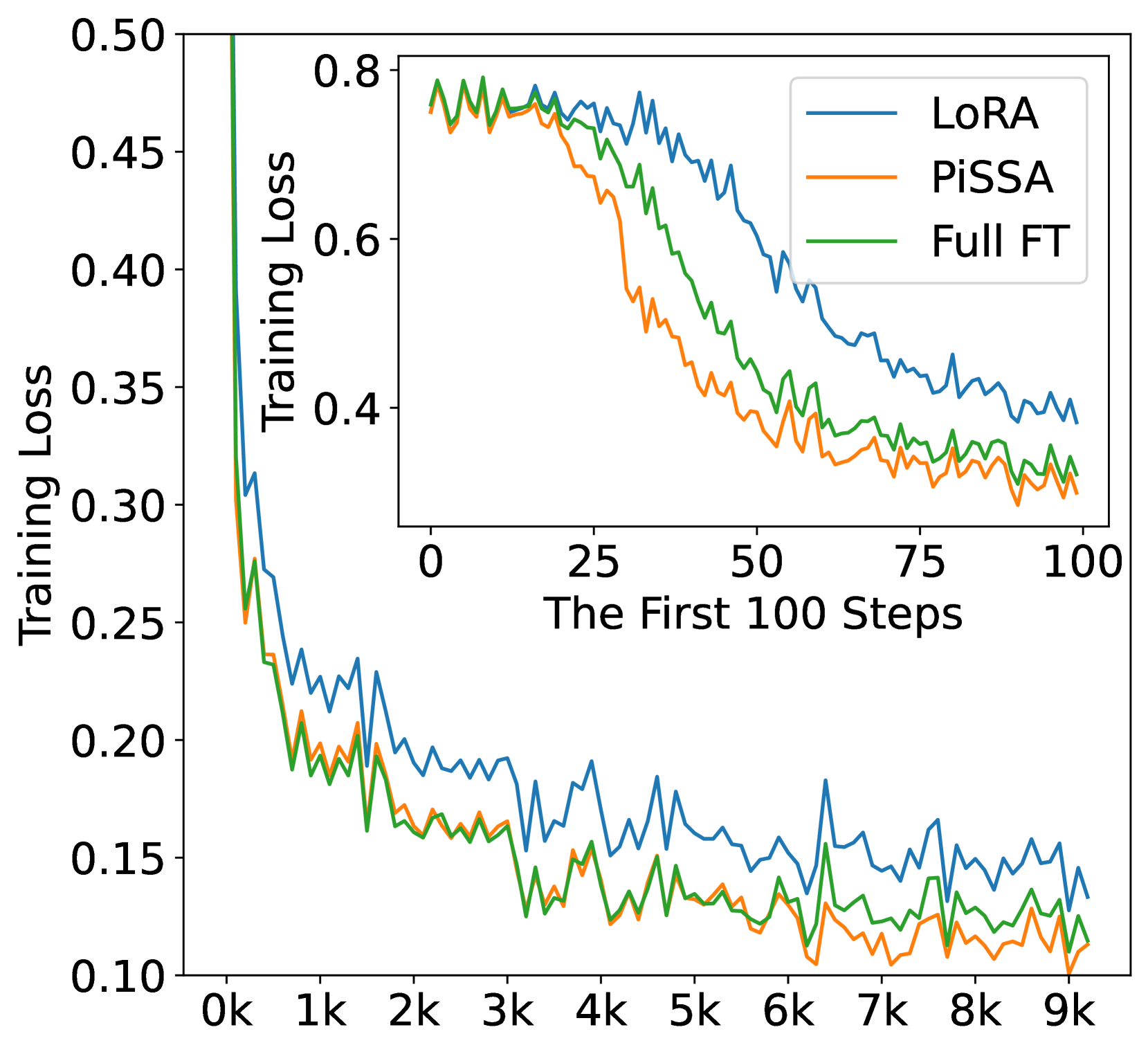
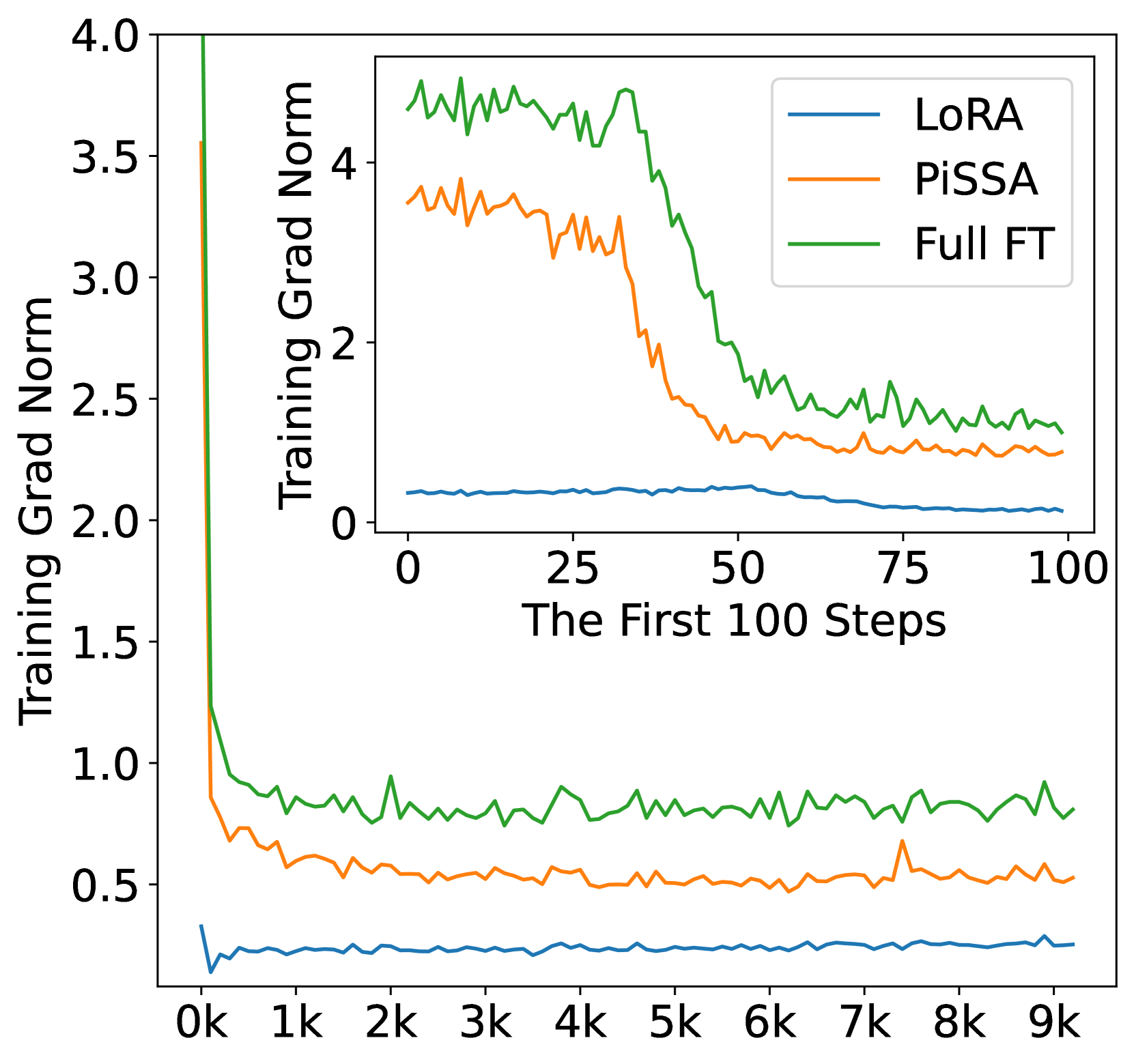
我们的 Principal Singular 值和 Singular 向量 Adapter (PiSSA) 与 LoRA 及其后续版本不同，它的 重点不是近似 $\mathrm{\Delta }W$，而是 $W$。我们对矩阵 $W$ 应用奇异值分解 (SVD)。根据奇异值的大小，我们将 $W$ 分成两部分：由几个最大奇异值组成的主低秩矩阵 $W^{pri}$ 和拥有其余较小奇异值的残差矩阵 $W^{res}$（数量较大，代表可能的长尾分布）。 主矩阵$W^{pri}$可以用$A\in {ℝ}^{m\times r}$和$B\in {ℝ}^{r\times n}$的乘积来表示，其中$r\ll \min (m,n)$。 如图1(c)所示，$A$和$B$基于主奇异值和奇异向量进行初始化，并且是可训练的。 相反，$W^{res}$ 使用残余奇异值和奇异向量的乘积进行初始化，并在微调期间保持冻结状态。 由于主奇异向量表示矩阵 $W$ 具有最显着拉伸或影响的方向，通过直接调整这些主成分，PiSSA 能够更快更好地拟合训练数据（如图所示） 2(a))。 此外，PiSSA的损失和梯度范数曲线在我们的实验中经常表现出与全参数微调类似的趋势（图4)，表明主成分的微调与在某种程度上对整个矩阵进行微调。

由于主要成分$W^{pri}$保留在适配器中并且具有全精度，PiSSA的另一个好处是，当对冻结部分$W^{res}$应用量化时，我们可以显着减少与 QLoRA（量化整个 $W$)相比的量化误差，如图 2(b) 所示。 因此，PiSSA 与量化完美兼容，使其成为 LoRA 的即插即用替代品。

2相关作品

具有数十亿参数的大型语言模型（大语言模型）的巨大复杂性和计算需求在使其适应特定下游任务时存在重大障碍。 参数高效微调 (PEFT) [12, 13] 通过最大限度地减少微调参数和内存需求，同时实现与完全微调相当的性能，成为一种引人注目的解决方案。 PEFT 包含部分微调 [14, 15, 16, 17, 18, 19, 20, 21]、软提示微调 [22, 23, 24, 25, 26, 27, 28]，非线性适配器微调[29, 30, 31, 32, 33, 34, 35, 36, 37, 38]，以及低阶基于适配器的微调[39,40,11,41]。

LoRA [11] 将可训练适配器注入线性层。 经过微调后，这些调整可以重新参数化到标准模型结构中，由于它们能够保持模型的原始架构，同时实现高效的微调，因此获得了广泛的采用。 继 LoRA 之后，AdaLoRA [42, 41, 43] 动态学习模型每一层中 LoRA 所需的秩大小。 DeltaLoRA [44, 45] 使用适配器层的参数更新模型的原始权重，增强 LoRA 的表示能力。 LoSparse [46] 结合了 LoRA 来防止剪枝消除过多的表达神经元。 DoRA [47]引入了幅度分量来学习$\mathrm{\Delta }W$的尺度，同时利用原始AB作为$\mathrm{\Delta }W$的方向分量。 与 LoRA 及其后继者专注于学习权重更新的低阶近似值不同，我们的 PiSSA 方法直接调整模型的基本但低阶部分，同时保持噪声较高、高阶和非必要部分冻结。 尽管我们的方法在理念上与 LoRA 不同，但它具有 LoRA 的大部分结构优势，并且可以通过这些方法进行扩展以提高其性能。

QLoRA [10] 将 LoRA 与 4 位 NormalFloat (NF4) 量化以及双量化和分页优化器集成在一起，可在单个 48GB GPU 上微调 65B 参数模型，同时保持性能完整的 16 位微调任务。 QA-LoRA [48]引入了分组运算符来增加低位量化的自由度。 LoftQ [49]通过分解QLoRA的量化误差矩阵并用适配器保留主成分来减少量化误差。 我们的 PiSSA 方法还可以与量化技术相结合，我们发现与 QLoRA 和 LoftQ 相比，PiSSA 显着降低了量化误差。

3 PiSSA：Principal 奇异值和奇异向量A适应

本节正式介绍我们的PrincipalS奇异值和S奇异向量A适应方法。 PiSSA 计算自注意力和多层感知器 (MLP) 层内矩阵 $W$ 的奇异值分解 (SVD)。 矩阵 $W\in {ℝ}^{m\times n}$ 的（经济规模）SVD 由 $W=US{V}^T$ 给出，其中 $U\in {ℝ}^{m\times \text{min}(m,n)},V\in {ℝ}^{n\times \text{min}(m,n)}$ 是具有正交列的奇异向量，$V^T$ 是 $V$ 的转置。 $S=\text{diag}(𝐬)\in {ℝ}^{\text{min}(m,n)\times \text{min}(m,n)}$，其中操作$\text{diag}(𝐬)$将$𝐬$变换为对角矩阵$S$,$𝐬\in {ℝ}_{\ge 0}^{\text{min}(m,n)}$表示奇异值按降序排列。 当顶部 $r$ 奇异值 ${𝐬}_{[:r]}$ 明显大于其余奇异值 ${𝐬}_{[r:]}$ 时，我们将 $W$ 的内在秩记作 $r$。因此，$S$ 与 $U$ 和 $V$ 可分为两组：主奇异值和向量-$\{U_{[:,:r]},S_{[:r,:r]},V_{[:,:r]}\}$，以及剩余奇异值和向量-$\{U_{[:,r:]},S_{[r:,r:]},V_{[:,r:]}\}$，其中矩阵切分符号与 PyTorch 中的相同，$[:r]$ 表示第一个 $r$ 维数。 主要奇异值和向量用于初始化由 $A\in {ℝ}^{m\times r}$ 和 $B\in {ℝ}^{r\times n}$ 组成的注入适配器：

$A$ $=U_{[:,:r]}{S}_{[:r,:r]}^{1/2}\in {ℝ}^{m\times r},$ (2)

$B$ $=S_{[:r,:r]}^{1/2}{V}_{[:,:r]}^T\in {ℝ}^{r\times n}.$ (3)

残差奇异值和向量用于构建残差矩阵，该矩阵在微调期间被冻结：

$$W^{res}=U_{[:,r:]}{S}_{[r:,r:]}{V}_{[:,r:]}^T\in {ℝ}^{m\times n}.$$ (4)

如方程5所示，$AB$与残差矩阵的整合也保留了预训练模型在微调开始时的全部能力：

$$Y=XW=X(W^{res}+W^{pri})=X(W^{res}+AB).$$ (5)

与LoRA类似，$A$和$B$的梯度也由$\frac{\partial L}{\partial A}=X^T\left(\frac{\partial L}{\partial Y}\right)B^T$和$\frac{\partial L}{\partial B}=A^T{X}^T\left(\frac{\partial L}{\partial Y}\right)$给出。 由于 ${𝐬}_{[:r]}$ $\gg$ 元素为 ${𝐬}_{[r:]}$ 元素，可训练适配器 $W^{pri}=AB$ 包含 $W$ 最基本的方向。在理想情况下，训练 $AB$ 反映了微调整个模型的过程，尽管使用的参数较少。 直接影响模型最重要部分的能力使 PiSSA 能够更快更好地收敛。 相反，LoRA 使用高斯噪声和零初始化适配器 $A$ 和 $B$，同时保持 $W$ 冻结。 因此，在微调的早期阶段，梯度很小或方向随机，可能会导致梯度下降步骤的大量浪费。 此外，较差的初始化可能会导致找到次优的局部最小点，从而导致更差的泛化性能。

由于 PiSSA 与 LoRA 具有相同的架构，因此它继承了 LoRA 的大部分优点。 这些包括但不限于通过减少可训练参数数量来微调模型的能力、量化残差模型以减少训练中前向传播期间的内存消耗以及易于部署。 该适配器简单的线性结构有助于在部署时将可训练矩阵与预训练权重集成，从而保持完全微调模型的原始推理速度。 采用快速SVD技术[50]允许PiSSA在几秒钟内完成初始化（附录B)，这是一个可以忽略不计的成本。

为了存储效率，我们可以选择不存储稠密参数矩阵$\mathrm{\Delta }W$，而是存储低秩矩阵$\mathrm{\Delta }A$和$\mathrm{\Delta }B$。 如附录C所示，单独利用$\mathrm{\Delta }A$和$\mathrm{\Delta }B$可以促进它们与原始预训练模型的无缝集成。 最后，一个预训练模型可以容纳多个 $\mathrm{\Delta }A,\mathrm{\Delta }B$，通过不同的 PiSSA 或 LoRA 程序进行微调，这使得预训练模型能够快速适应不同的下游应用。

4 QPiSSA：带量化的 PiSSA

量化将矩阵的值范围划分为几个连续的区域，并将落在一个区域内的所有值映射为相同的“量化”值。 这是一种减少前向传播内存消耗的有效技术，但在反向传播过程中就失效了。 同时，LoRA 极大地降低了后向内存需求，使其非常适合同时使用 LoRA 和量化，其中对基本模型进行量化以实现内存高效的前向传播，并且 LoRA 适配器保持完全精度以获得准确的后向参数更新。 之前的一项代表性工作 QLoRA 将基础模型量化为普通浮点 4 位 (NF4)，并使用高斯零初始化来初始化全精度 $A$ 和 $B$。 因此，总误差由下式给出：

$$\text{Quantization Error of QLoRA}={\Vert W-\left(nf4(W)+AB\right)\Vert }_{\ast }={\Vert W-nf4(W)\Vert }_{\ast },$$ (6)

其中${\Vert M\Vert }_{\ast }$表示核范数（也称为迹范数）[51]，定义为：

$${\Vert M\Vert }_{\ast }=\mathrm{trace}\left(\sqrt{M^{\ast }M}\right)=\sum _{i=1}^{\min \{m,n\}}{\sigma }_i(M),$$ (7)

其中 ${\sigma }_i(M)$ 是 $M$ 的 $i^{\text{th}}$ 奇异值。我们可以看到，QLoRA 的量化误差与直接量化基础模型的误差相同。 然而，我们的 QPiSSA 不量化基本模型，而是量化残差模型。 因此，其误差由下式给出：

$$\text{Quantization Error of QPiSSA}={\Vert W-\left(nf4(W^{res})+AB\right)\Vert }_{\ast }={\Vert W^{res}-nf4(W^{res})\Vert }_{\ast }.$$ (8)

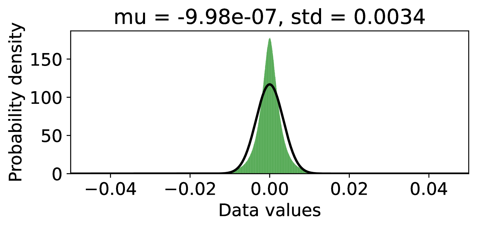
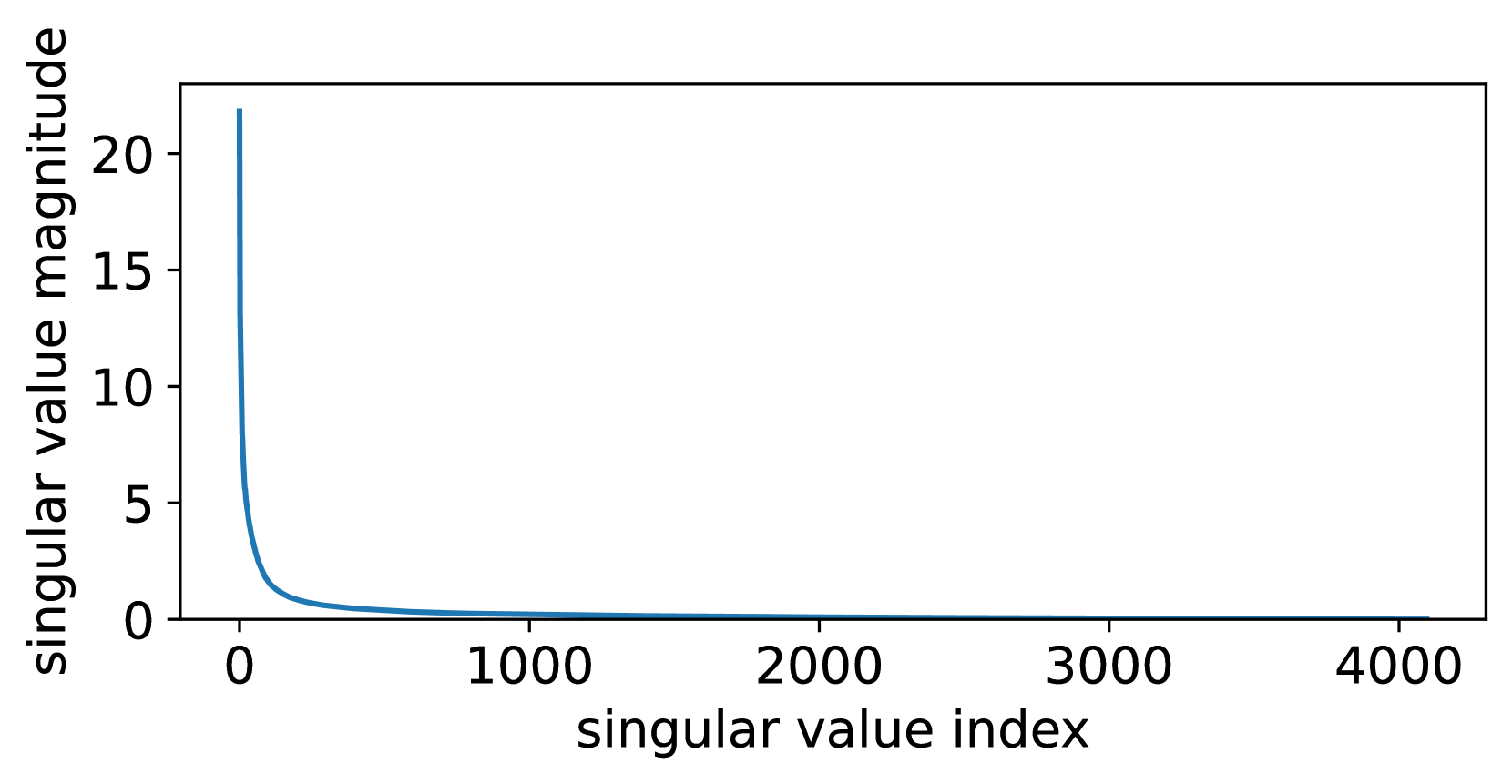
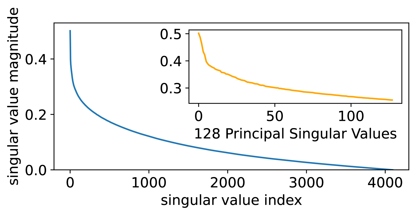
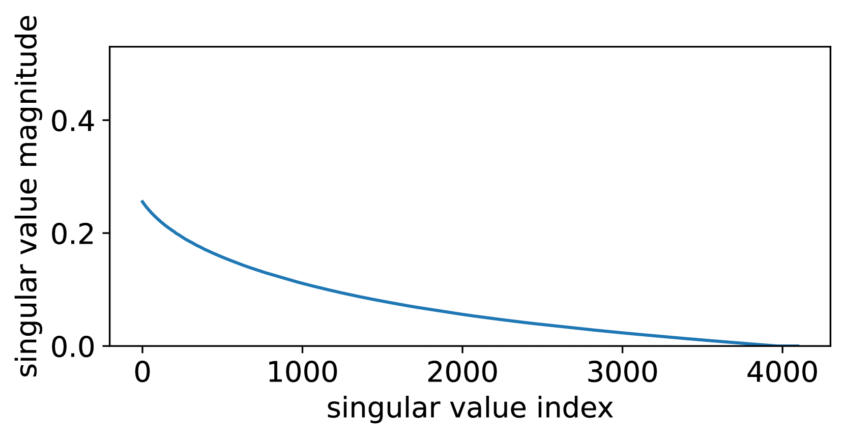
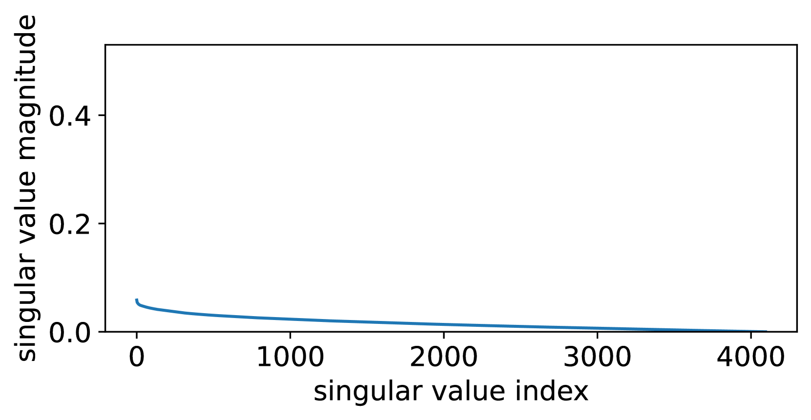
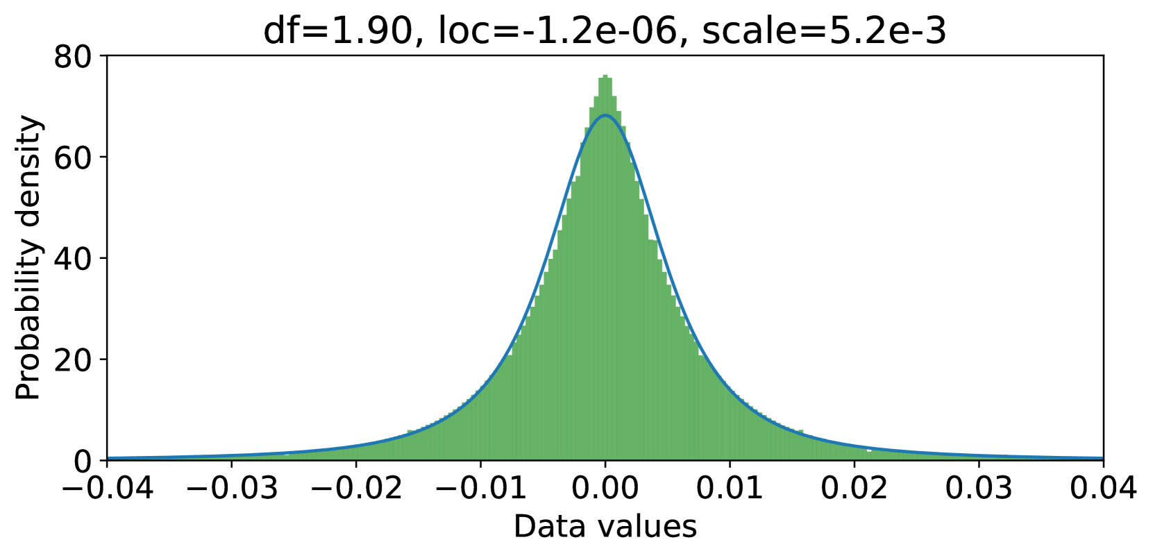
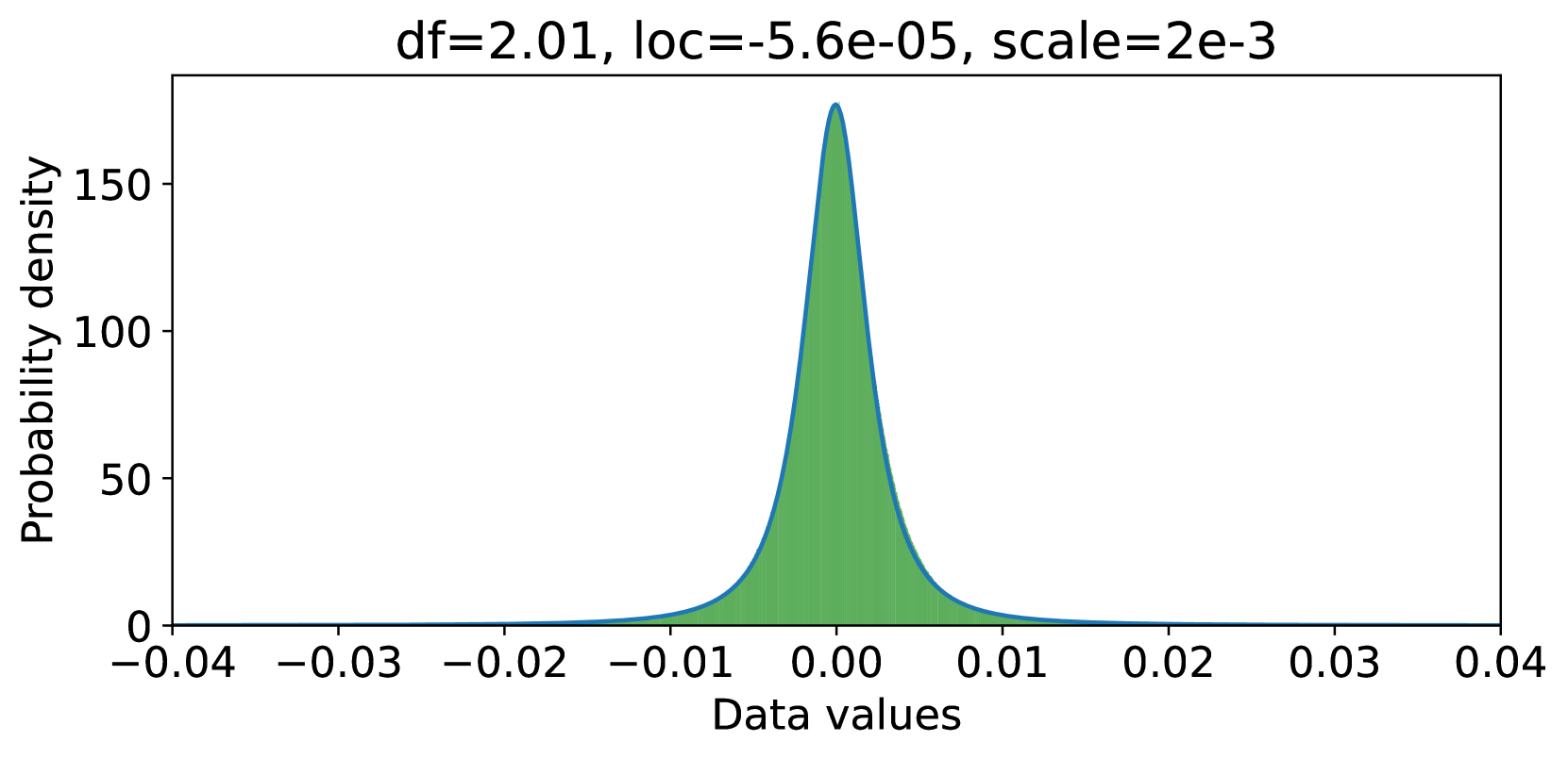
Since the residual model has removed the large-singular-value components, $W^{res}$ has a narrower distribution than that of $W$, as can be seen in Figures 3(a) and 3(b) (comparing the singular value distributions of $W$ and $W^{res}$), as well as Figures 3(c) and 3(f) (comparing the value distributions of $W$ and $W^{res}$), which is beneficial for reducing the quantization error. 此外，由于 NF4 针对正态分布数据 [10] 进行了优化，因此我们分别对 $W$ 和 $W^{res}$ 的值拟合高斯分布。 从图 3(c) 和 3(f) 中可以看出，$W^{res}$ 更接近高斯分布，并且具有更小的标准差，使得将 NF4 更适合应用于 $W^{res}$ 而不是 $W$。上述两种方法都使得 QPiSSA 的量化误差明显低于 QLoRA，如图 3(d) 和 3(e) 所示。

(a) Original matrix $W$

(b) Residual matrix $W^{res}$

(c) The distribution of $W$

(d) Error matrix of QLoRA

(e) Error matrix of QPiSSA

(f) The distribution of $W^{res}$

图3： 图(a)、(b)、(d)和(e)按降序可视化$W$、$W^{res}$、$W-nf4(W)$和$W^{res}-nf4(W^{res})$ LLaMA 2-7B 的“layers[0].self_attn.q_proj”矩阵。 图(c)和(f)显示了$W$和$W^{res}$的数据值分布。

除了减少量化误差的优点外，QPiSSA 的梯度方向与 PiSSA 相似，因此与 QLoRA 相比，其微调性能明显更好。

5实验

实验在NVIDIA A800-SXM4(80G) GPU上进行。 在我们的实验中，我们采用Alpaca [52]实现策略，使用AdamW优化器，批量大小为128，学习率为2e-5，余弦退火计划，预热比率为0.03 ，没有任何重量衰减。 正如 QLoRA [10] 的 B.3 节中所讨论的，我们仅使用来自指令跟踪数据集的响应来计算损失。 我们确保 lora_alpha 始终等于 lora_r，将 lora_dropout 设置为 0，并将适配器合并到基础模型的所有线性层中。 我们将 Float32 计算类型用于 LoRA 和 PiSSA 中的基本模型和适配器。 对于 QLoRA、LoftQ 和 QPiSSA，我们使用 4 位 NormalFloat [10] 作为基本模型，使用 Float32 作为适配器。 BFloat16 [53]用于全参数微调，以节省资源（参见附录D)。

5.1 评估 PiSSA 在 NLG 和 NLU 任务上的性能

表1给出了自然语言生成（NLG）任务上微调策略PiSSA、LoRA和全参数微调的比较评估。 我们对 LLaMA 2-7B [54]、Mistral-7B-v0.1 [55] 和 Gemma-7B [56] 进行了微调> 在 MetaMathQA 数据集 [2] 上评估他们在 GSM8K [57] 和 MATH [2] 验证集上解决数学问题的能力。 此外，模型在 CodeFeedback 数据集 [58] 上进行了微调，并使用 HumanEval [59] 和 MBPP [60] 评估编码熟练程度t2> 数据集。 此外，模型在 WizardLM-Evol-Instruct 数据集 [7] 上进行训练，并在 MT-Bench 数据集 [6] 上测试会话能力。 所有实验均使用包含 100K 数据点的子集进行，并且仅训练一个 epoch 以减少开销。

表格1： 在 NLG 任务上比较 PiSSA 和 LoRA

Model	Strategy	Trainable	GSM8K	MATH	HumanEval	MBPP	MT-Bench
		Parameters
LLaMA 2-7B	Full FT	6738M	49.05	7.22	21.34	35.59	4.91
	LoRA	320M	42.30	5.50	18.29	35.34	4.58
	PiSSA	320M	53.07	7.44	21.95	37.09	4.87
Mistral-7B	Full FT	7242M	67.02	18.6	45.12	51.38	4.95
	LoRA	168M	67.70	19.68	43.90	58.39	4.90
	PiSSA	168M	72.86	21.54	46.95	62.66	5.34
Gemma-7B	Full FT	8538M	71.34	22.74	46.95	55.64	5.40
	LoRA	200M	74.90	31.28	53.66	65.41	4.98
	PiSSA	200M	77.94	31.94	54.27	66.17	5.64

如表1所示，在所有模型和任务中，使用 PiSSA 进行微调的性能始终优于使用 LoRA 进行微调的性能。 例如，使用 PiSSA 对 LLaMA、Mistral 和 Gemma 进行微调，在数学任务中的性能分别提高了 10.77%、5.26% 和 3.04%。 在编码任务中，改进分别为 20%、6.95% 和 1.14%。 在 MT-Bench 中，我们观察到提高了 6.33%、8.98% 和 13.25%。 值得注意的是，在编码任务中，使用仅占 Gemma 2.3% 可训练参数的 PiSSA 比全参数微调的性能高出 15.59%。 进一步的实验表明，这种改进在不同数量的训练数据和历元（第 5.2 节）中都是稳健的，包括 4 位精度和全精度（第 5.3 节）、不同模型大小和类型(5.4 节），以及不同比例的可训练参数(5.5 节）。

表2： 在 NLU 任务上比较 PiSSA 和 LoRA。 详情请参阅附录I。

Method	Parameters	MNLI	SST-2	MRPC	CoLA	QNLI	QQP	RTE	STS-B
RoBERTa-large (355M)
Full FT	355M	90.2	96.4	90.9	68.0	94.7	92.2	86.6	91.5
LoRA	1.84M	90.6	96.2	90.9	68.2	94.9	91.6	87.4	92.6
PiSSA	1.84M	90.7	96.7	91.9	69.0	95.1	91.6	91.0	92.9
DeBERTa-v3-base (184M)
Full FT	184M	89.90	95.63	89.46	69.19	94.03	92.40	83.75	91.60
LoRA	1.33M	90.65	94.95	89.95	69.82	93.87	91.99	85.20	91.60
PiSSA	1.33M	90.43	95.87	91.67	72.64	94.29	92.26	87.00	91.88

我们还使用 RoBERTa-large [62] 和 DeBERTa-v3-base [63 在 GLUE 基准 [61] 上评估 PiSSA 的自然语言理解 (NLU) 能力]。 表 2 显示了使用两个基本模型执行的 8 项任务的结果。 PiSSA 在 16 个实验设置中的 14 个上优于 LoRA，并且在 QQP + RoBERTa 上实现了相同的性能。 唯一的例外是 MNLI 数据集上基于 DeBERTa 的模型。 在审查训练损失后，我们发现 PiSSA 在最后一个时期的平均损失 $0.17$ 低于 LoRA 的 $0.24$。 这表明PiSSA的拟合能力仍然强于LoRA。

5.2 使用完整数据和更多纪元的实验

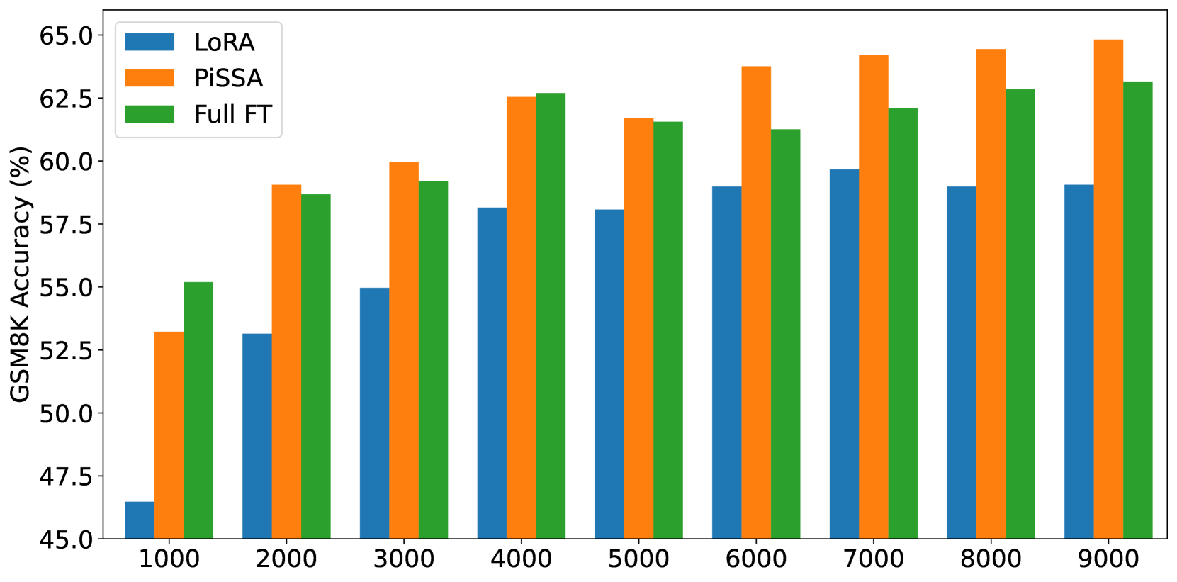
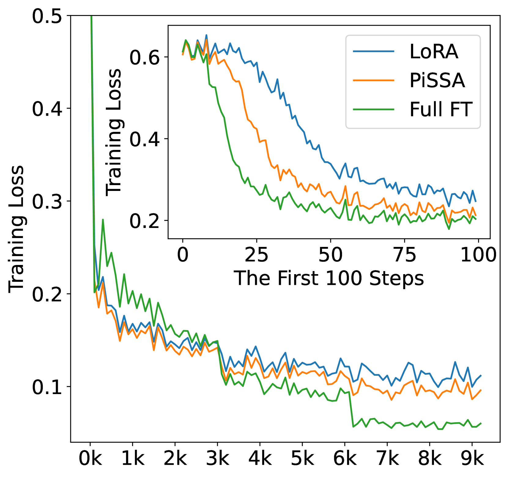
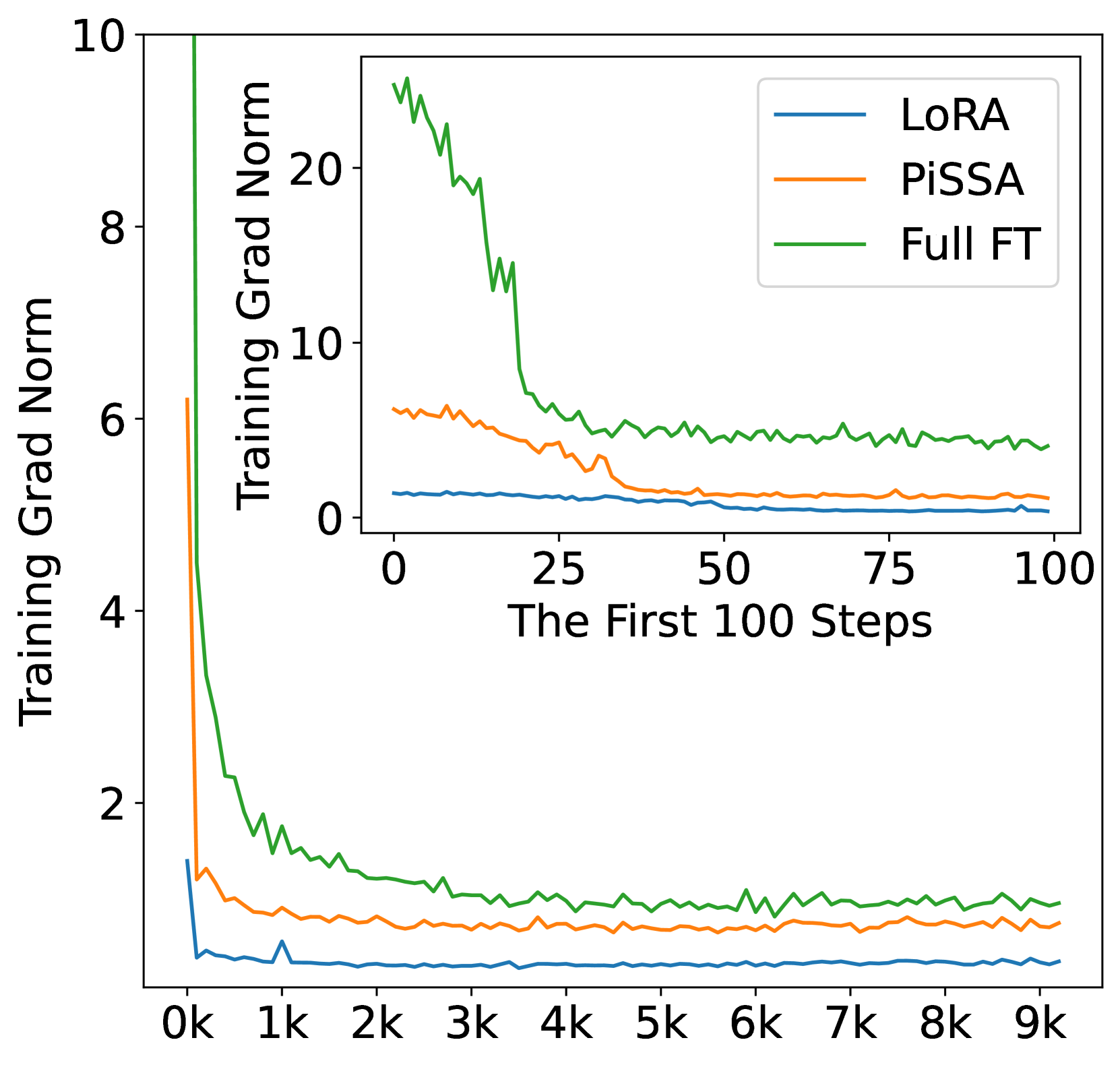
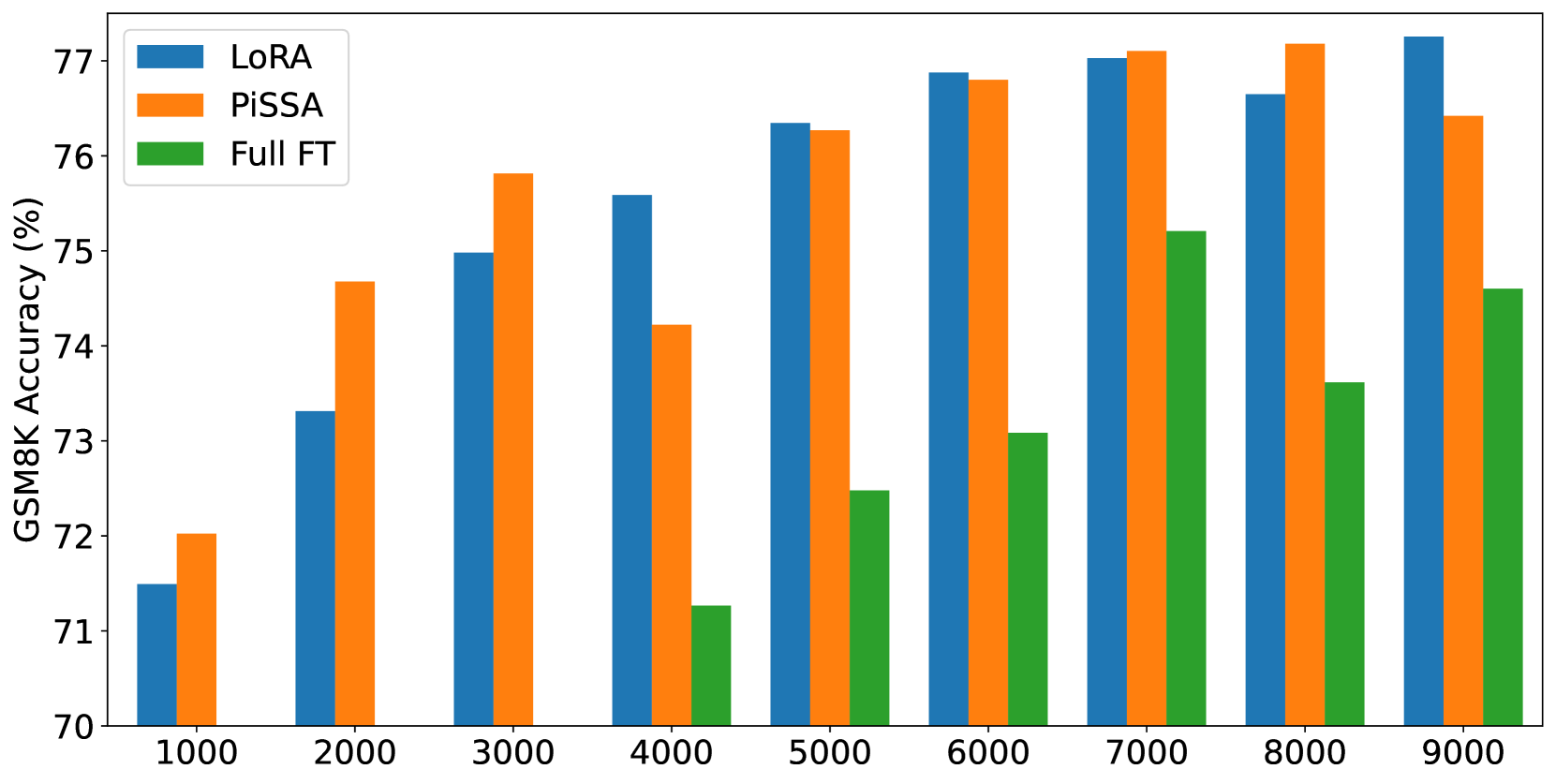
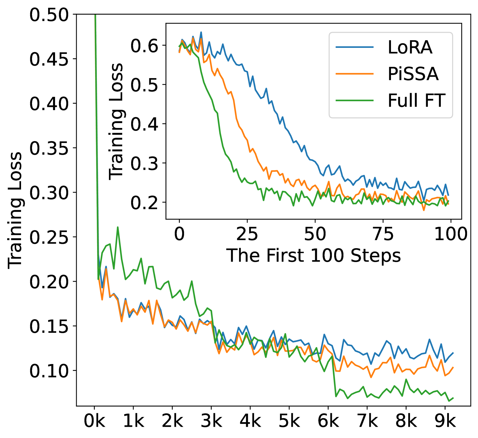
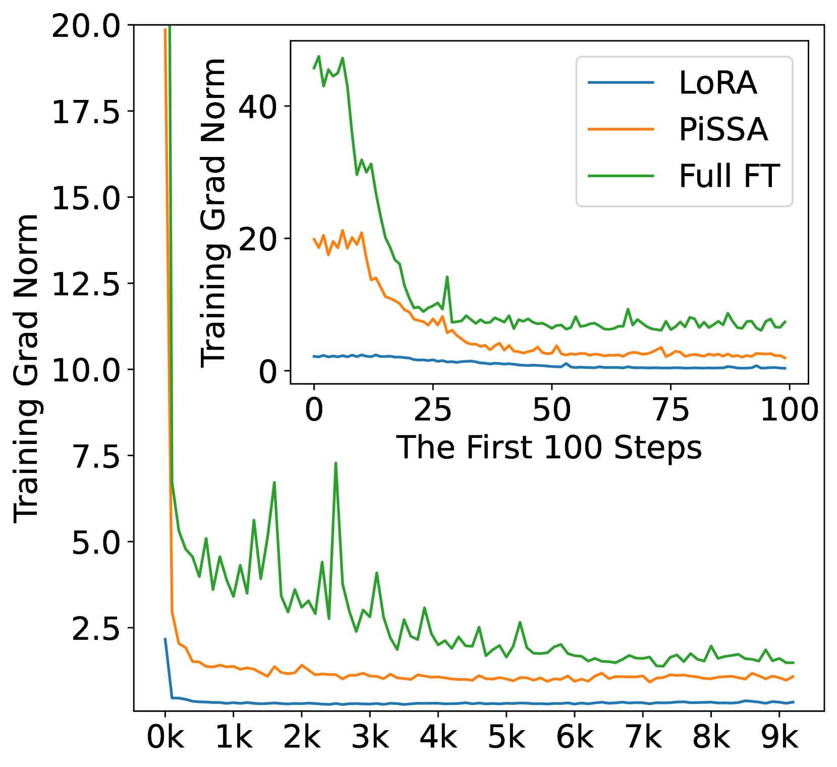
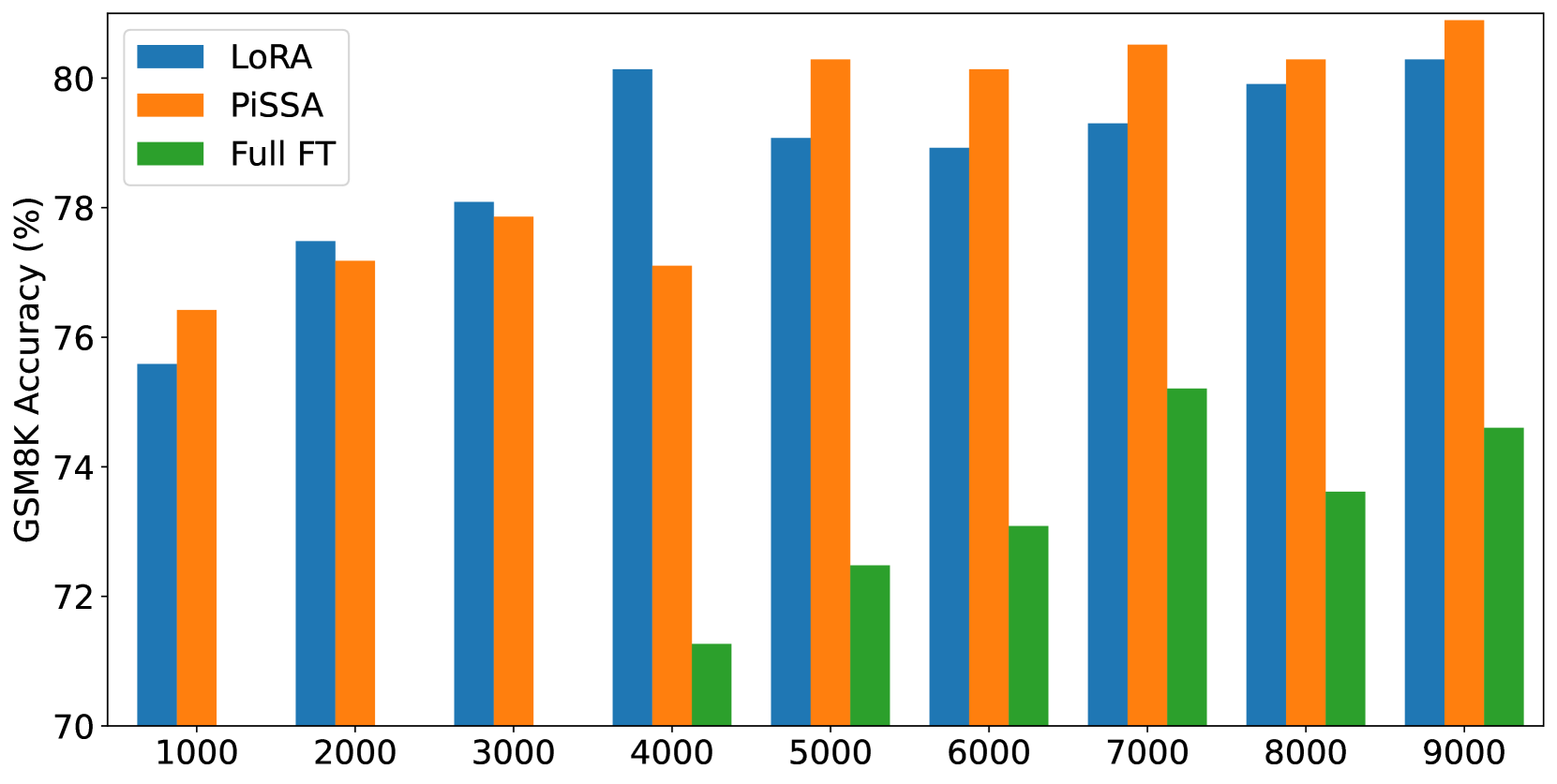
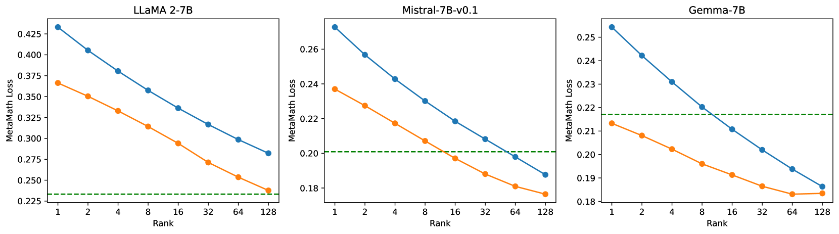
在本节中，我们在完整的 MetaMathQA-395K 数据集上对 LLaMA 2-7B 模型进行 3 个周期的微调，以确保彻底饱和。 训练损失和梯度范数被可视化，以展示更快的收敛速度，并在 GSM8K 数据集上每 1000 步进行评估，以展示 PiSSA 与 LoRA 相比的卓越性能。 结果如图4所示。 此外，附录G详细介绍了 Mistral-7B 和 Gemma-7B 的类似比较。

(a) Loss over steps.

(b) Grad norm over steps.

(c) Accuracy on GSM8K over training steps.

图4： LoRA（以蓝色表示）、PiSSA（以橙色表示）和全参数微调（以绿色表示）的训练步骤的损失、梯度范数和评估精度。

根据图4(a)，PiSSA的损失在前100步中迅速减小，PiSSA的梯度范数（如图4(b)所示）为明显高于LoRA，趋势类似全微调。 在整个过程中，PiSSA 的损失始终低于 LoRA，这表明 PiSSA 收敛到了更好的局部最优。 如图4(c)所示，与LoRA相比，PiSSA始终实现了更高的精度，并且在大多数情况下还超越了全参数微调。 我们假设这是因为 PiSSA 是完全微调的去噪版本。 比较PiSSA和全微调的梯度范数和损失曲线，我们可以看到，全微调的梯度范数较大并没有带来较低的损失，这表明梯度范数的一部分花在了对噪声不利的方向上。减少损失。 这一现象与图2(a)一致。

5.3进行4位量化实验

在本节中，我们首先比较PiSSA、QLoRA和LoftQ的初始量化误差降低率。 该比率定义为$(1-\frac{{\Vert W-(nf4(W^{{}^{\prime }})+AB)\Vert }_{\ast }}{{\Vert W-nf4(W)\Vert }_{\ast }})\times 100\%$，测量与直接量化基础模型相比，每种方法实现的相对误差降低。 部分结果见表3，完整结果见附录E表6。

表3： QLoRA、LoftQ 和 PiSSA 跨不同层的量化误差降低率。

	Method	Rank	Q	K	V	O	Gate	Up	Down	AVG
LLaMA 2-7B	QLoRA	–	0	0	0	0	0	0	0	0
	loftQ	128	16.5	16.5	15.9	16.0	12.4	12.4	12.3	14.6
	PiSSA	128	27.9	27.2	18.7	18.6	15.8	13.6	13.6	19.4
LLaMA 3-8B	QLoRA	–	0	0	0	0	0	0	0	0
	loftQ	128	16.4	29.8	28.8	16.1	11.9	11.7	11.7	18.1
	PiSSA	128	26.3	41.7	32.3	20.1	14.4	12.5	12.9	22.9
LLaMA 3-70B	QLoRA	–	0	0	0	0	0	0	0	0
	LoftQ	64	6.1	17.8	17.0	6.0	4.3	4.4	4.2	8.5
	PiSSA	64	15.7	34.2	18.9	7.5	6.7	5.7	4.7	13.4
	PiSSA	128	23.2	49.0	30.5	12.5	10.1	8.8	8.2	20.3

在表3中，与直接量化基础模型相比，PiSSA 将量化误差降低了约 20%。 对于低阶矩阵，这种减少更为显着。 例如，在 LLaMA-3-70B [64] 中，所有“关键”投影层都减少了 49%。 表 3 中的结果验证了第 4 节中讨论的 QLoRA 不会减少量化误差。 相比之下，PiSSA 在减少量化误差方面明显优于 LoftQ，如附录 F 中进一步讨论。

除了减少量化误差之外，我们预计 QPiSSA 的收敛速度也比 QLoRA 和 LoftQ 更快。 我们使用 LoRA/QLoRA、PiSSA/QPiSSA、LoftQ 训练 LLaMA 3-8B，并在 MetaMathQA-395K 上进行 3 个周期的完全微调，并记录 GSM8K 上的损失、梯度范数和准确性。

(a) Loss over training steps.

(b) Grad norm over training steps.

(c) Accuracy on GSM8K over training steps.

图5： (Q)LoRA、(Q)PiSSA、LoftQ 和全参数微调训练步骤的损失、梯度范数和评估精度。

根据图5，QPiSSA在前100步的损失降低速度甚至比PiSSA和完全微调还要快。 LoftQ虽然可以降低量化误差，但其损失收敛速度并不比LoRA和QLoRA快，说明QPiSSA降低量化误差的能力和快速收敛的能力也可能是正交能力。 经过充分训练后，QPiSSA 的损失也远低于 LoRA/QLoRA 和 LoftQ。 梯度范数明显大于 LoRA/QLoRA 和 LoftQ 的梯度范数。 在微调性能方面，QPiSSA的精度高于QLoRA和LoftQ，甚至优于全精度LoRA。

5.4各种尺寸和类型模型的实验

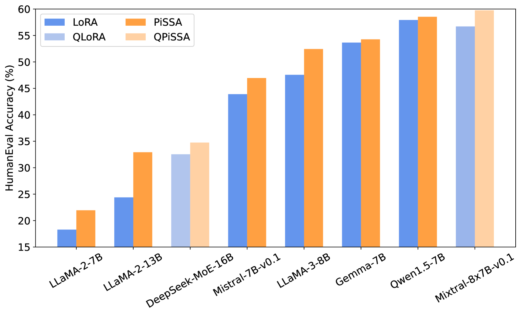
在本节中，我们比较了 9 个模型的 (Q)PiSSA 和 (Q)LoRA，参数范围为 7-70B，包括 LLaMA 2-7/13B [54]、LLaMA-3-8/ 70B [64]、Mistral-7B [55]、Gemma-7B [56] 和 Qwen1.5-7B [ 65]、Yi-1.5-34B [66] 和 MoE 模型：DeepSeek-MoE-16B [67] 和 Mixtral-8x7B [68 ]。 这些模型在 MetaMathQA-100K 和 CodeFeedback-100K 数据集上进行了微调，并在 GSM8K 和 HumanEval 上进行了评估。 DeepSeek-MoE-16B、Mixtral-8x7B、Yi-1.5-34B 和 LLaMA-3-70B 使用 QPiSSA 和 QLoRA 进行微调，而其他模型则使用 PiSSA 和 LoRA。 从图6中可以看出，与（Q）LoRA相比，（Q）PiSSA在各种尺寸和类型的模型上都显示出更高的精度，展示了其相对于（Q）LoRA的一致优势。

图6： 7B 到 70B 模型中 (Q)PiSSA 和 (Q)LoRA 的比较。

5.5各个等级的实验

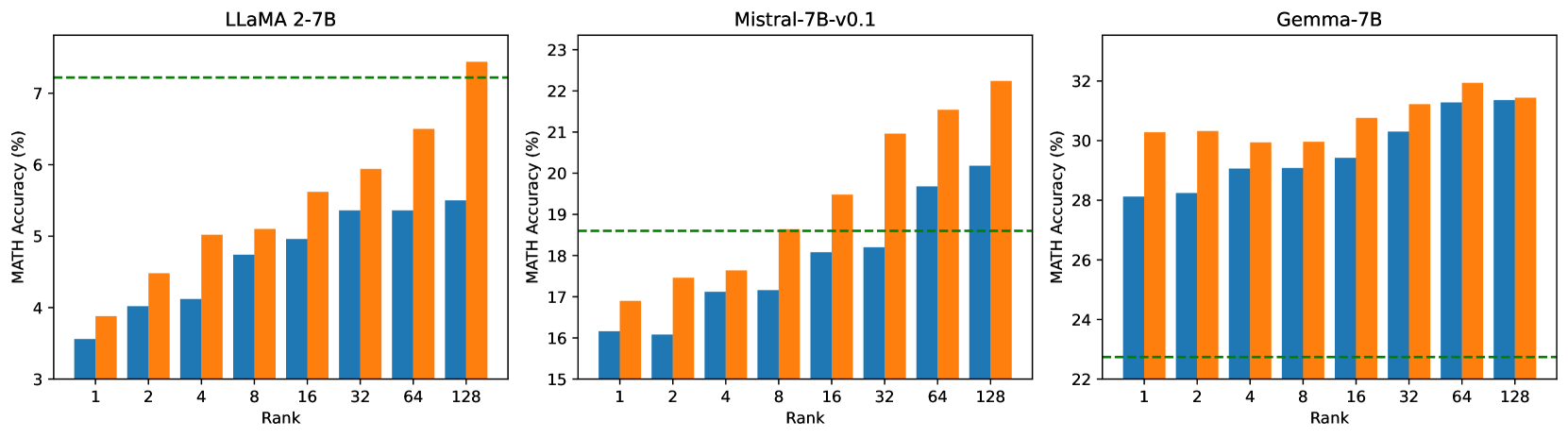
本节探讨将 PiSSA/QPiSSA 和 LoRA/QLoRA 的排名从 1 逐步增加到 128 的影响，旨在确定 PiSSA/QPiSSA 在不同排名下是否始终优于 LoRA/QLoRA。 训练使用 MetaMathQA-100K 数据集进行 1 epoch，而验证则在 GSM8K 和 MATH 数据集上进行。 这些实验的结果如图7所示，其他结果在附录H中给出。

(a) Quantization error reduction ratio across ranks.

(b) Training loss under various ranks.

(c) Accuracy on GSM8K under various ranks.

(d) Accuracy on MATH under various ranks.

图7： (Q)LoRA、(Q)PiSSA、LoftQ 之间的比较以及跨等级的全面微调。

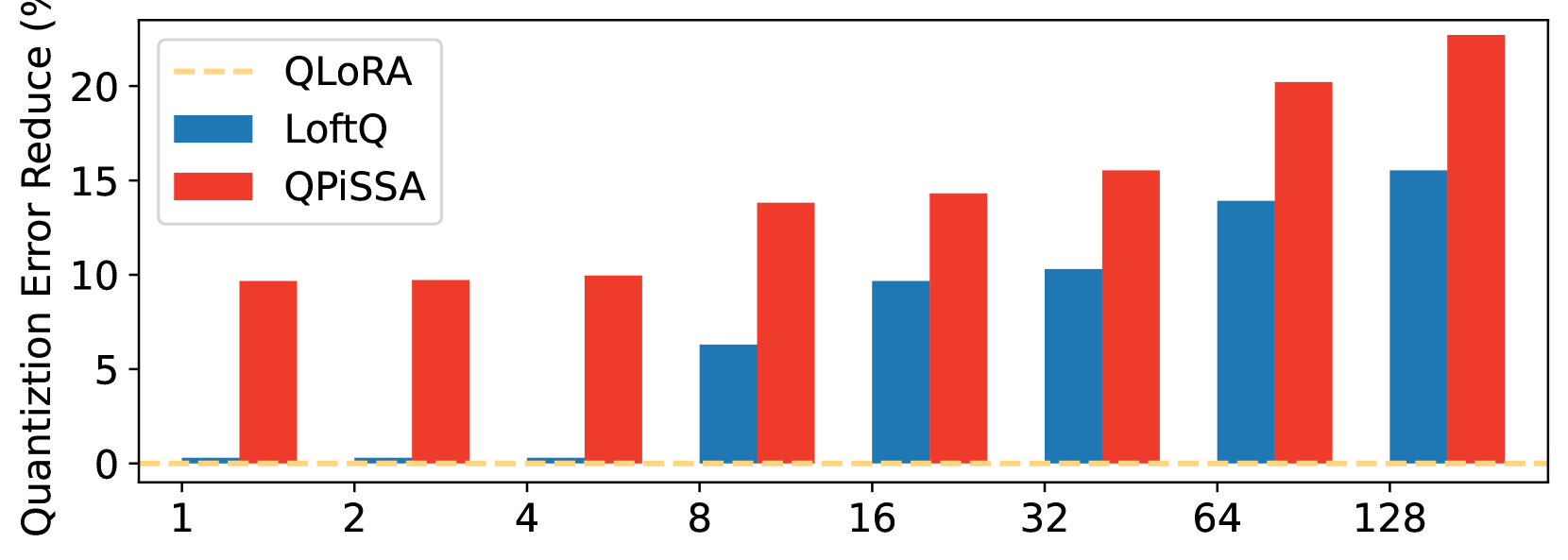
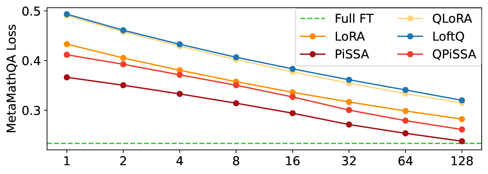
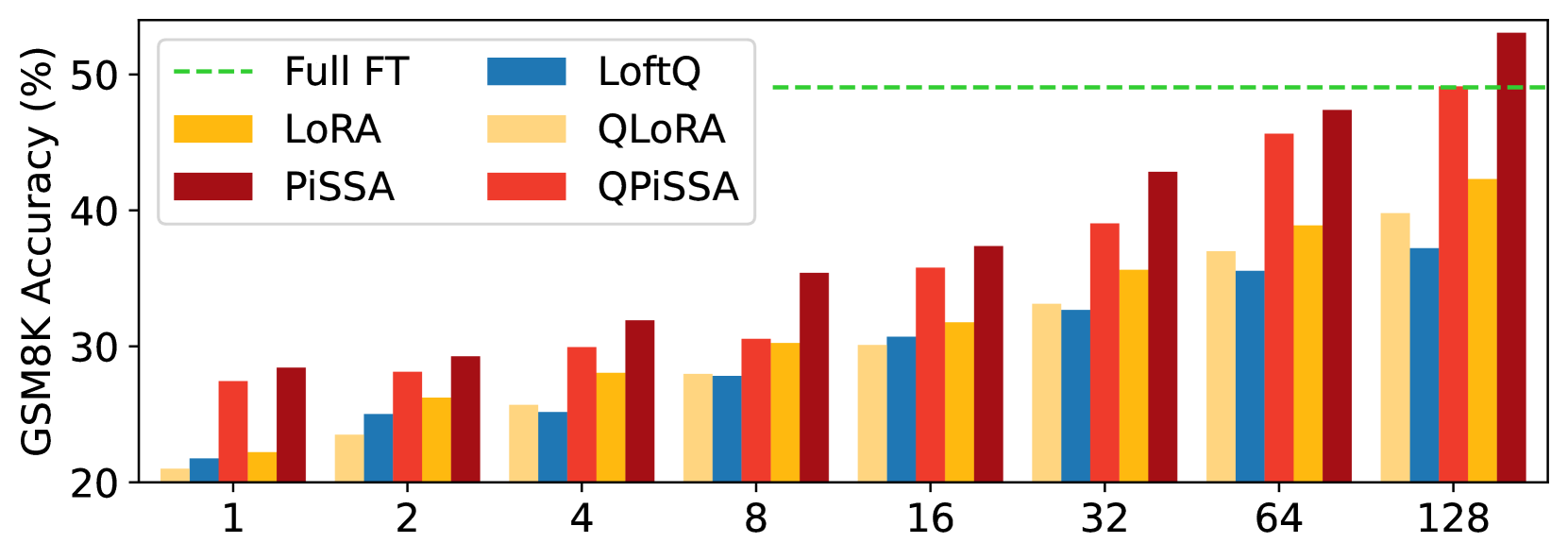
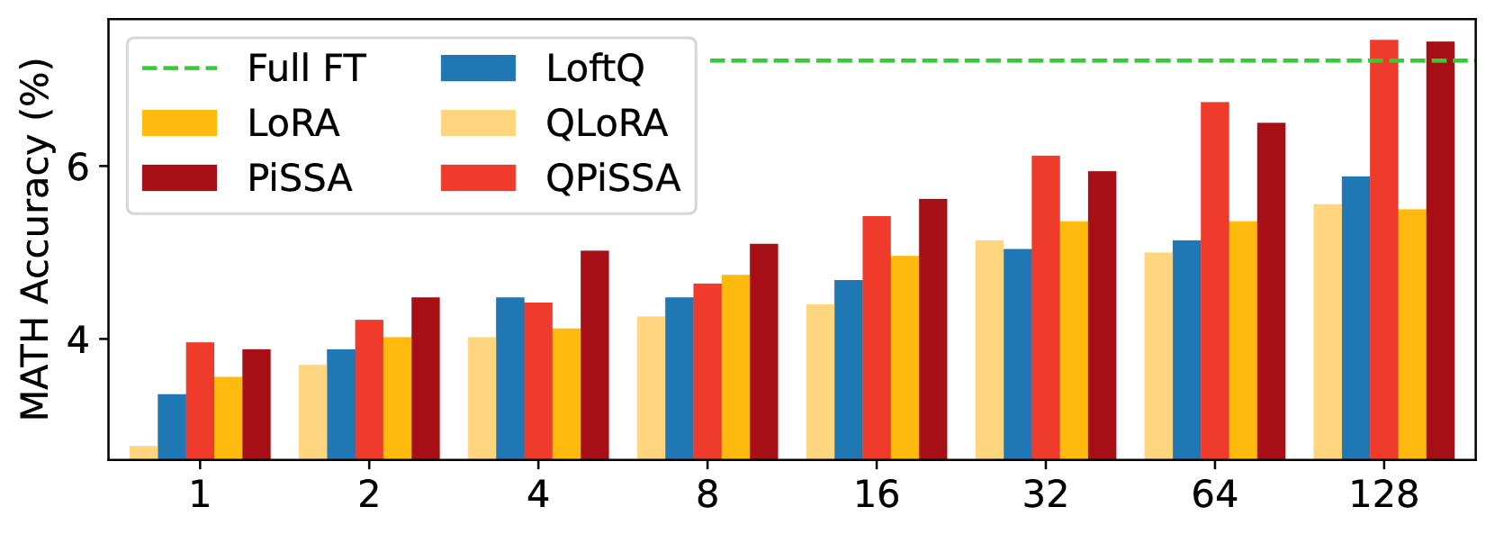
图7(a)说明了不同等级的量化误差减少率。 在该图中，QLoRA 显示量化误差没有减少，而 QPiSSA 在减少所有级别的量化误差方面始终优于 LoftQ，在较低级别的优势尤其明显。 在图7(b)中，显示了等级范围从1到128训练的模型的训练集的最终损失。 结果表明，与 LoRA、QLoRA 和 LoftQ 相比，PiSSA 和 QPiSSA 能够更好地拟合训练数据。 在图7(c)和图7(d)中，我们比较了不同等级下的微调模型在GSM8K和MATH验证集上的准确性，发现在相同数量的可训练参数下，PiSSA 的性能始终优于 LoRA。 此外，随着Rank的提高，PiSSA将达到并超越全参数微调的性能。

6结论

本文提出了一种 PEFT 技术，将奇异值分解 (SVD) 应用于预训练模型的权重矩阵。 从SVD获得的主成分用于初始化一个名为PiSSA的低秩适配器，而剩余成分保持冻结，以同时实现有效的微调和参数效率。 通过大量实验，我们发现 PiSSA 及其 4 位量化版本 QPiSSA 在 NLG 和 NLU 任务中、跨不同训练步骤、各种模型大小和类型以及各种可训练参数下的性能显着优于 LoRA 和 QLoRA。 PiSSA 通过识别和微调模型中的主要成分，为 PEFT 的研究提供了一个新颖的方向，类似于切片并重新烘烤最丰富的披萨片。 由于 PiSSA 与 LoRA 具有相同的架构，因此它可以作为一种高效的替代初始化方法无缝地用于现有的 LoRA 管道中。

7限制

PiSSA 还有一些问题没有在本文中解决：1）除了语言模型之外，PiSSA 还可以适应卷积层并增强视觉任务的性能吗？ 2）PiSSA是否也可以从LoRA的一些改进中受益，例如自适应调整排名的AdaLoRA [69]和DyLoRA [42]？ 3）我们能否为PiSSA相对于LoRA的优势提供更多的理论解释？ 这些问题我们正在积极探索。 尽管如此，我们很高兴看到 PiSSA 在现有实验中已经展现出巨大的潜力，并期待社区提供更多测试和建议。

论文的补充材料

“PiSSA：大语言模型的主奇异值和奇异向量适应”。

• 在A节中，我们比较了使用高、中、低奇异值和向量来初始化适配器。 实验结果表明，使用主奇异值和向量初始化适配器可产生最佳的微调性能。

• 在B节中，我们使用快速奇异值分解来初始化PiSSA。 结果表明，快速奇异值分解的性能在短短几秒内就接近了 SVD 分解的性能。 这确保了从 LoRA/QLoRA 转换到 PiSSA/QPiSSA 的成本可以忽略不计。

• 在C节中，我们演示了经过训练的PiSSA适配器可以无损地转换为LoRA，从而允许与原始模型集成，促进共享，并允许使用多个PiSSA适配器。

• 在第D节中，我们探讨了使用不同精度的实验效果。

• 在E节中，我们讨论了QPiSSA在多轮SVD分解过程中的效果，它可以在不增加训练或推理成本的情况下显着减少量化误差。

• 在F节中，我们对QLoRA、LoftQ和QPiSSA之间的量化误差进行了全面的比较，从理论上解释了为什么QPiSSA可以减少量化误差。

• 在 G 部分中，我们训练了 Mistral-7B 和 Gemma-7B 足够数量的步骤。 结果表明，与全参数微调相比，PiSSA 和 LoRA 不太容易出现过拟合。

• 在H节中，我们对不同级别的PiSSA和LoRA进行了更详细的比较。 很明显，PiSSA 在损失收敛、量化误差减少和不同等级的最终性能方面始终优于 LoRA。

• 在第I节中，我们描述了NLU任务的详细设置。

附录A各种SVD元件的导电实验

为了研究不同大小的奇异值和向量对微调性能的影响，我们使用主奇异值、中奇异值和次奇异值初始化注入 LLaMA 2-7B、Mistral-7B-v0.1 和 Gemma-7B 的适配器值和向量。 然后，这些模型在 MetaMathQA 数据集 [2] 上进行微调，并根据 GSM8K [57] 和 MATH 数据集 [70] 进行评估，结果如图8所示。

图8： 使用主奇异值、中奇异值和次奇异值和向量进行初始化，分别报告三个模型的 MetaMathQA 训练损失以及 GSM8K 和 MATH 验证集的准确性。

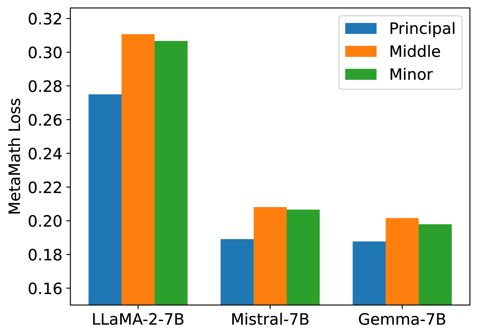
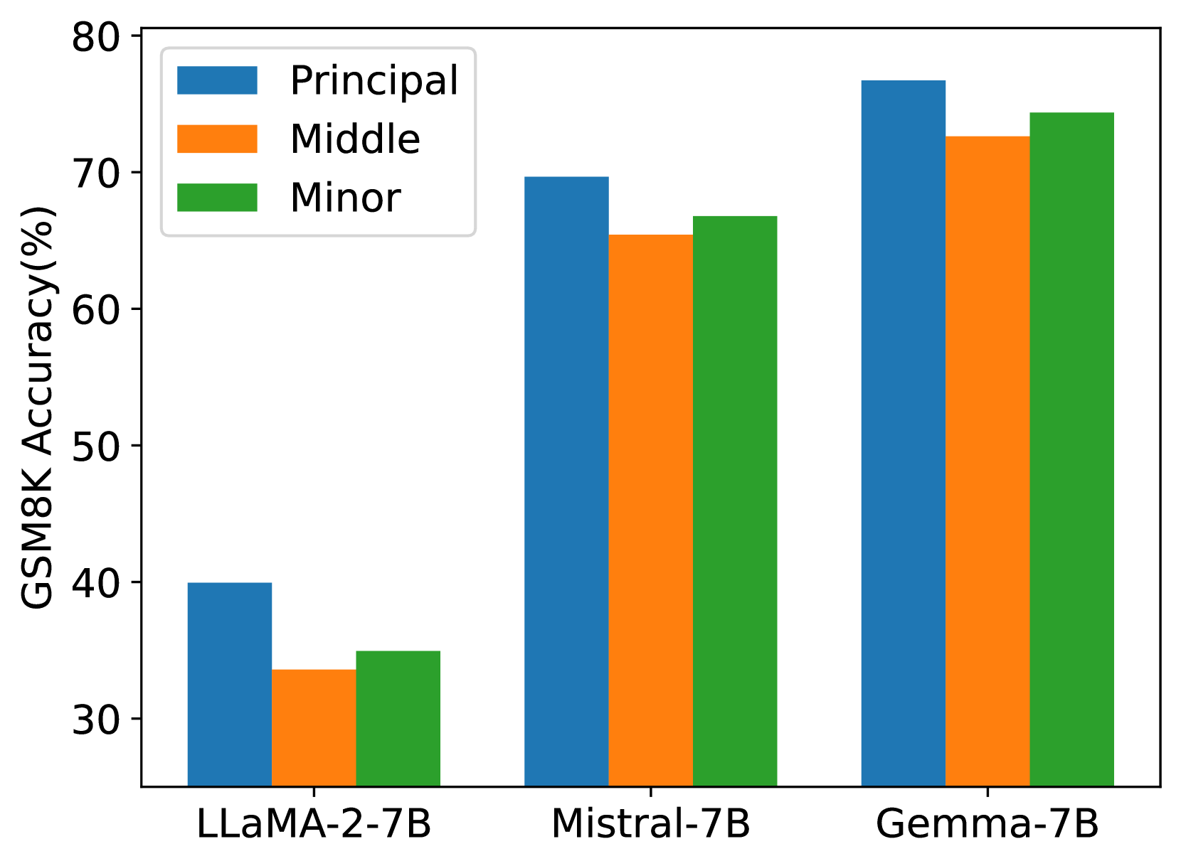
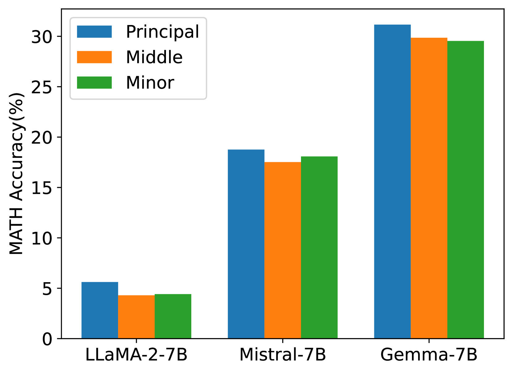
结果强调，使用主奇异值和向量初始化适配器始终可以减少所有三个模型的 GSM8K 和 MATH 验证数据集上的训练损失并提高准确性。 这强调了我们的策略在基于主奇异值微调模型参数方面的有效性。

附录B快速奇异值分解

为了加速预训练矩阵$W$的分解，我们采用了Halko等人提出的算法[50]（记为Fast SVD），该算法引入了随机性来实现近似矩阵分解。 我们比较了 SVD 和 Fast SVD 的初始化时间、误差和训练损失，结果如表B所示。初始化时间是指分解预训练参数矩阵$W$所需的计算时间，以秒为单位。 初始化误差表示 Fast SVD 与分解矩阵后的 SVD 相比引入的差异的大小。 具体来说，误差是原始SVD和Fast SVD分解的矩阵之间的绝对差之和。 对于错误，我们在表中报告了自注意力模块的结果。 损失是指训练结束时的损失值。 在 Fast SVD 中，参数 niter 指的是要进行的子空间迭代次数。 硝石越大，分解时间越长，但分解误差越小。 符号$\mathrm{\infty }$表示SVD方法的实验结果。

表 4： SVD 和 Fast SVD 在初始化时间、误差和训练损失方面的比较。

Metric	Niter	Rank
		1	2	4	8	16	32	64	128
Initialize Time	1	5.05	8.75	5.07	8.42	5.55	8.47	6.80	11.89
	2	4.38	4.71	4.79	4.84	5.06	5.79	7.70	16.75
	4	5.16	4.73	5.09	5.16	5.60	7.01	7.90	11.41
	8	4.72	5.11	5.14	5.40	5.94	7.80	10.09	14.81
	16	6.24	6.57	6.80	7.04	7.66	9.99	14.59	22.67
	$\mathrm{\infty }$	434.92	434.15	434.30	435.42	435.25	437.22	434.48	435.84
Initialize Error	1	1.30E-3	1.33E-3	1.55E-3	1.9E-3	1.98E-3	1.97E-3	2.00E-3	1.93E-3
	2	5.84E-4	1.25E-3	1.45E-3	1.43E-3	1.48E-3	1.55E-3	1.48E-3	1.33E-3
	4	6.01E-4	8.75E-4	6.75E-4	1.10E-3	1.05E-3	1.03E-3	1.08E-3	9.75E-4
	8	1.26E-4	2.34E-4	5.25E-4	7.25E-4	5.75E-4	8.25E-4	8.25E-4	7.75E-4
	16	7.93E-5	2.25E-4	1.28E-4	6.50E-4	4.25E-4	6.50E-4	6.00E-4	4.75E-4
	$\mathrm{\infty }$	–	–	–	–	–	–	–	–
Training Loss	1	0.3629	0.3420	0.3237	0.3044	0.2855	0.2657	0.2468	0.2301
	2	0.3467	0.3337	0.3172	0.2984	0.2795	0.2610	0.2435	0.2282
	4	0.3445	0.3294	0.3134	0.2958	0.2761	0.2581	0.2414	0.2271
	8	0.3425	0.3279	0.3122	0.2950	0.2753	0.2571	0.2406	0.2267
	16	0.3413	0.3275	0.3116	0.2946	0.2762	0.2565	0.2405	0.2266
	$\mathrm{\infty }$	0.3412	0.3269	0.3116	0.2945	0.2762	0.2564	0.2403	0.2264

It can be observed that the computation time of the SVD is tens of times that of Fast SVD. In addition, SVD exhibits consistently high time consumption with minimal variation as the rank increases, while Fast SVD, although experiencing a slight increase in computation time with higher ranks, remains significantly lower compared to SVD throughout. As the rank increases, the initialization error initially rises gradually, with a slight decrease observed when the rank reaches 128. And at the same rank, increasing the niter in Fast SVD leads to a gradual reduction in error. For training loss, we observed that as the rank increases, the training loss decreases gradually. At the same rank, with the increase of niter, the training loss of models initialized based on Fast SVD approaches that of models initialized based on SVD.

Appendix C Equivalently Converting PiSSA into LoRA

The advantage of PiSSA lies in its ability to significantly enhance training outcomes during the fine-tuning phase. After training, it allows for the direct sharing of the trained matrices $A$ and $B$. However, if we directly save $A,B$, users need to perform singular value decomposition on the original model to get $W^{res}$, which requires additional time. When employing fast singular value decomposition, there can be slight inaccuracies too. More importantly, such a way necessitates altering the parameters of the original model, which can be inconvenient when using multiple adapters, especially when some adapters might be disabled or activated. Therefore, we recommend converting the trained PiSSA module equivalently into a LoRA module, thereby eliminating the need to modify the original model’s parameters during sharing and usage. In the initialization phase, PiSSA decomposes the original matrix into principal components and a residual matrix: $W=W^{res}+AB$. Upon completion of training, the model adjusts the weights as follows: $W+\mathrm{\Delta }W=W^{res}+A^{\prime }{B}^{\prime }$. Thus, the modification of the model weights by PiSSA is given by:

$\mathrm{\Delta }W$ $=A^{\prime }{B}^{\prime }-AB$ (9)

$=\underset{\mathrm{\Delta }A}{\underbrace{[A^{\prime }A]}}\underset{\mathrm{\Delta }B}{\underbrace{\left[\begin{array}{c}{B}^{\prime }\\ -B\end{array}\right]}}$ (10)

where $\mathrm{\Delta }A\in {ℝ}^{m\times 2r}$ and $\mathrm{\Delta }B\in {ℝ}^{2r\times n}$. Therefore, we can store and share the new adaptor $\mathrm{\Delta }A$ and $\mathrm{\Delta }B$ instead of $A^{\prime },B^{\prime }$, which allows directly inserting the adaptor to the original matrix and avoids breaking $W$. Since $r$ is typically small, the twice storage overhead is still acceptable. This modification allows for plug-and-play usage without the need for singular value decomposition, saving time and avoiding computational errors associated with the SVD, without necessitating changes to the original model parameters.

Appendix D Comparison of Fine-Tuning in BF16 and FP32 Precision

In this section, we compare the effects of training with BFloat16 and Float32 precision. The comparing include four models: LLaMA-2-7B, Mistral-7B, Gemma-7B, and LLaMA-3-8B, each fine-tuned with all parameters in both BFloat16 and Float32 precision on the MetaMathQA-395K dataset. The validation results conducted on the GSM8K dataset are shown in Figure 5.

Table 5: Comparison of fine-tuning results of LLaMA-2-7B, Mistral-7B, Gemma-7B, and LLaMA-3-8B in BF16 and FP32 precision on MetaMathQA-395K dataset for 3 epochs.

Model	Training Loss		GSM8K ACC (%)		MATH ACC (%)
	BF16	FP32	BF16	FP32	BF16	FP32
LLaMA-2-7B	0.1532	0.1316	63.15	68.31	13.14	20.38
Mistral-7B	0.1145	0.1306	73.09	65.88	26.44	23.66
Gemma-7B	0.1331	0.1382	75.21	75.97	29.18	28.64
LLaMA-3-8B	0.1271	0.1317	81.96	75.44	33.16	28.72

From Table 5, it is evident that the choice of precision greatly affects the experimental results. For example, the LLaMA-2-7B model shows a 5.16% higher performance on the GSM8K dataset when using FP32 compared to BF16. Conversely, the Mistral-7B and LLaMA-3-8B on GSM8K are 7.21% and 6.52% lower with FP32 than with BF16 separately. The Gemma-7B model shows similar performance with both precisions. Unfortunately, the experiments did not prove which precision is better. To reduce training costs, we use BF16 precision when fine-tuning all parameters. For methods with lower training costs, such as LoRA, PiSSA, we use FP32 precision. For QLoRA, QPiSSA and LoftQ, the base model was used NF4 precision, while the adapter layers used FP32 precision.

Appendix E Reducing Quantization Error through QPiSSA with Multiple Iteration of SVD

Table 6 provides a supplementary explanation of the results in Table 3. When number of iterations $T>1$, LoftQ uses an $N$-bit quantized weight $Q\in {ℝ}_N^{m\times n}$ and low-rank approximations $A\in {ℝ}^{m\times r}$ and $B\in {ℝ}^{n\times r}$ to minimize the following objective by alternating between quantization and singular value decomposition:

$\underset{Q,A,B}{\min }{\Vert W-(Q+A{B}^{\top })\Vert }_F,$ (11)

where $\parallel \cdot {\parallel }_F$ denotes the Frobenius norm, $A$ and $B$ are set to zero. Inspired by LoftQ, our QPiSSA $T$-iter alternately minimize the following objective:

$\underset{W_{res},A,B}{\min }{\Vert W-(nf4(W_{res})+A{B}^{\top })\Vert }_F,$ (12)

where $A$ and $B$ are initialized by the principal singular values and singular vectors. The process is summarized in Algorithm 1:

Algorithm 1 QPiSSA-$T$-iters, $T\ge 2$

0: Pre-trained weight $W$, target rank $r$, 4-bit quantization function $nf4(\cdot )$, alternating step $T$

1: Initialize $A_0,B_0\leftarrow \text{SVD}(W)$ by (2) and (3)

2: Initialize residual weight $W_{res}\leftarrow W-A_0{B}_0^{\top }$

3: for t = $2$ to $T$ do

4: Update $A_t,B_t\leftarrow \text{SVD}(W-nf4(W_{res}))$ by (2) and (3)

5: Update residual weight $W_{res}\leftarrow W-A_{t-1}{B}_{t-1}^{\top }$

6: end for

6: $nf4(W_{res}),A_T,B_T$

Table 6: PiSSA reduces more quantization error on various ranks and number of iterations.

	Method	Rank	niter	Q	K	V	O	Gate	Up	Down	AVG
LLaMA -2-7B	QLoRA	–	–	0	0	0	0	0	0	0	0
	loftQ	128	1	8.1	8.1	7.2	7.3	5.3	5.1	5.1	6.6
	PiSSA	128	1	19.0	18.1	8.9	8.9	8.2	5.9	6.0	10.7
	loftQ	128	5	16.5	16.5	15.9	16.0	12.4	12.4	12.3	14.6
	PiSSA	128	5	27.9	27.2	18.7	18.6	15.8	13.6	13.6	19.4
LLaMA -3-8B	QLoRA	–	–	0	0	0	0	0	0	0	0
	LoftQ	64	1	4.3	11.0	9.9	3.9	2.7	2.5	2.6	5.3
	PiSSA	64	1	11.3	16.4	8.8	6.3	4.5	2.9	3.3	7.7
	loftQ	64	5	10.1	18.8	18.2	9.9	7.1	7.1	7.1	11.2
	PiSSA	64	5	17.1	27.3	19.5	12.1	8.9	7.2	7.6	14.3
	loftQ	128	1	8.2	20.7	18.8	7.5	5.2	4.8	4.9	10.0
	PiSSA	128	1	17.1	26.5	10.7	10.7	7.0	5.0	5.6	11.8
	loftQ	128	5	16.4	29.8	28.8	16.1	11.9	11.7	11.7	18.1
	PiSSA	128	5	26.3	41.7	32.3	20.1	14.4	12.5	12.9	22.9
LLaMA -3-70B	QLoRA	–	–	0	0	0	0	0	0	0	0
	LoftQ	64	1	2.4	11.6	9.2	1.9	1.8	1.7	1.3	4.3
	PiSSA	64	1	12.3	25.0	9.0	4.1	4.2	3.2	2.2	8.6
	LoftQ	64	5	6.1	17.8	17.0	6.0	4.3	4.4	4.2	8.5
	PiSSA	64	5	15.7	34.2	18.9	7.5	6.7	5.7	4.7	13.4
	PiSSA	128	1	17.7	36.6	15.7	6.7	5.8	4.5	3.8	13.0
	PiSSA	128	5	23.2	49.0	30.5	12.5	10.1	8.8	8.2	20.3

According to Table 6, multiple iterations can significantly reduce quantization error. For instance, using QPiSSA-r64 with 5-iter on LLaMA-3-8B reduces the quantization error nearly twice as much as with 1-iter. In the main paper, we used 5 iterations in Section 5.3 and Section 5.4, while 1 iteration was used in Section 5.5.

Appendix F Comparing the Quantization Error of QLoRA, LoftQ and QPiSSA

This section extends the discussion in Section 4 by providing a comprehensive comparison of the quantization errors associated with QLoRA, LoftQ, and QPiSSA. Using the “layers[0].self_attn.q_proj” of LLaMA 2-7B as an example, we illustrate the singular values of critical matrices during the quantization process with QLoRA, LoftQ, and PiSSA in Figure 9. A larger sum of the singular values (nuclear norm) of the error matrix indicates a greater quantization error.

(a) Original matrix $W$

(b) Quantized matrix $nf4(W)$

(c) Residual matrix $W^{res}$

(d) Error of QLoRA

(e) Error of LoftQ

(f) Error of PiSSA

Figure 9: Several important singular values for calculation the quantization error of QLoRA, LoftQ and PiSSA.

The quantization error of QLoRA, which quantizes the base model to Normal Float 4-bit (NF4) and initializes $A$ and $B$ with Gaussian-Zero initialization, is:

$$\text{Quantization Error of QLoRA}={\Vert W-\left(nf4(W)+AB\right)\Vert }_{\ast }={\Vert W-nf4(W)\Vert }_{\ast },$$ (13)

As shown in Equation 13, QLoRA decomposes the original matrix in Figure 8(a) into the sum of a quantized matrix (Figure 8(b)) and an error matrix (Figure 8(d)). By comparing Figure 8(a) and Figure 8(d), we can see that the magnitude of the error matrix is much smaller than that of the original matrix. Therefore, the benefit of preserving the principal components of the $W$ matrix with the adapter is greater than that of preserving the principal components of the error matrix with the adapter.

LoftQ [49], designed to preserve the principal components of the error matrix using the adapter, first performs singular value decomposition on the quantization error matrix of QLoRA:

$$U^{err}{S}^{err}{V}^{err}=W-nf4(W),$$ (14)

then uses the larger singular values to initialize $A$ and $B$, thereby reducing the quantization error to:

$$Loft{Q}^{err}=||W-(nf4(W)+AB)||\ast =||U_{[r:]}^{err}{S}_{[r:,r:]}^{err}{V}_{[r:]}^{err}||\ast =\sum _{i=r}^{min(m,n)}{S}_{[i,i]}^{err}.$$ (15)

LoftQ eliminates only the largest $r$ singular values $S_{[:r]}^{\text{err}}$ (see Figure 8(e)) from the QLoRA error matrix (Figure 8(d)).

Our PiSSA, however, does not quantify the base model but the residual model:

$$\text{Quantization Error of PiSSA}={\Vert W-\left(nf4(W^{res})+AB\right)\Vert }_{\ast }={\Vert W^{res}-nf4(W^{res})\Vert }_{\ast },$$ (16)

where $A$ and $B$ are initialized following Equation 2 and 3. Since the residual model has removed the large-singular-value components, the value distribution of $W^{res}$ can be better fitted by a Student’s t-distribution with higher degrees of freedom compared to $W$ (as can be seen in Figure 10) and thus quantizing $W^{res}$ results in lower error using 4-bit NormalFloat (shown in Figure 8(f)).

(a) The original matrix $W$

(b) The residual matrix $W_{r}es$

Figure 10: Fitting the original matrix and the residual matrix using Student’s t-distribution.

Appendix G Evaluating PiSSA on Mixtral and Gemma with More Training Steps

This is the supplement for Section 5.2. We applied PiSSA, LoRA, and full parameter fine-tuning on the full MetaMathQA-395K dataset using Mistral-7B and Gemma-7B models, training for 3 epochs. Figures 11 and 12 display the training loss, gradient norm, and evaluation accuracy on GSM8K.

(a) Loss over training steps.

(b) Grad norm over steps.

(c) Accuracy on GSM8K over training steps.

Figure 11: Fine-tuning Mistral-7B-v0.1 on the MetaMathQA-395K dataset for 3 epochs: A comparison of full parameter fine-tuning (indicated by a dashed line), LoRA (in blue), and PiSSA (in orange).

(a) Loss over training steps.

(b) Grad norm over steps.

(c) Accuracy on GSM8K over training steps.

Figure 12: Fine-tuning Gemma-7B on the MetaMathQA-395K dataset for 3 epochs: A comparison of full parameter fine-tuning (indicated by a dashed line), LoRA (in blue), and PiSSA (in orange).

As shown in Figure 10(a) and 11(a), the loss for full parameter fine-tuning decreases sharply with each epoch, indicating overfitting to the training data. Notably, during the entire first epoch, the loss for full parameter fine-tuning on Mistral and Gemma is significantly higher than for LoRA and PiSSA, suggesting that full parameter fine-tuning has weaker generalization capabilities compared to LoRA and PiSSA on Mistral-7B and Gemma-7B models. The gradient norm for the first epoch in Figure 11(b) fluctuates dramatically with each step, further indicating instability in the training process for full parameter fine-tuning. Consequently, as illustrated in Figures 10(c) and 11(c), the performance of full parameter fine-tuning is markedly inferior to that of LoRA and PiSSA. These experiments demonstrate that using parameter-efficient fine-tuning can prevent the over-fitting issue caused by over-parameters.

Appendix H Supplementary Experiments on Various Ranks

H.1 Quantization Error for More Type of Layers

Figure 7(a) only shows the reduction ratio of quantization error for “q_proj” layers. In Figure 13, we present the error reduction ratios for the remaining types of linear layers under different ranks.

Figure 13: Comparison of quantization errors in QLoRA, LoftQ, and PiSSA across k_proj, v_proj, o_proj and gate_proj, up_proj, down_proj layers.

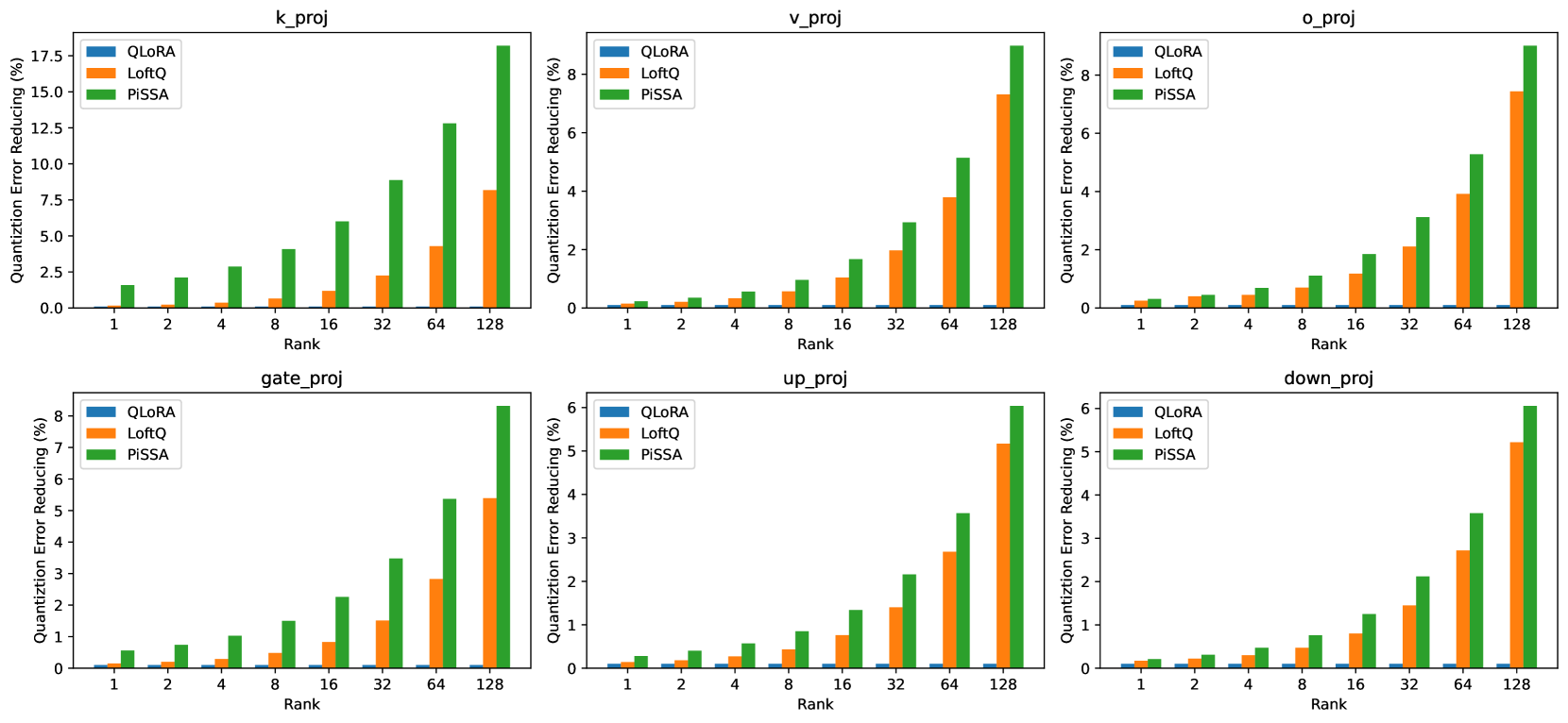
From Figure 13 it can be observed that under different ranks, the reduction ratio of quantization error for various linear layers in LLaMA-2-7B, including “k_proj”, “v_proj”, “o_proj”, “gate_proj”, “up_proj”, and “down_proj” layers, is consistently lower with PiSSA compared to LotfQ.

H.2 Evaluation Performance for More Model on Various Ranks

Section 5.5 only validated the effectiveness of LLaMA-2-7B. In Figure 14, we also present the comparative results of Mistral-7B-v0.1, and Gemma-7B under different ranks.

(a) Final training loss across different ranks.

(b) Rank-wise performance evaluated using pass@1 on the GSM8K dataset.

(c) Rank-wise performance evaluated using pass@1 on the MATH dataset.

Figure 14: Fine-tuning LLaMA 2-7B, Mistral-7B-v0.1, and Gemma-7B on the MetaMathQA dataset: A comparison of full parameter fine-tuning (indicated by a dashed line), LoRA (in blue), and PiSSA (in orange).

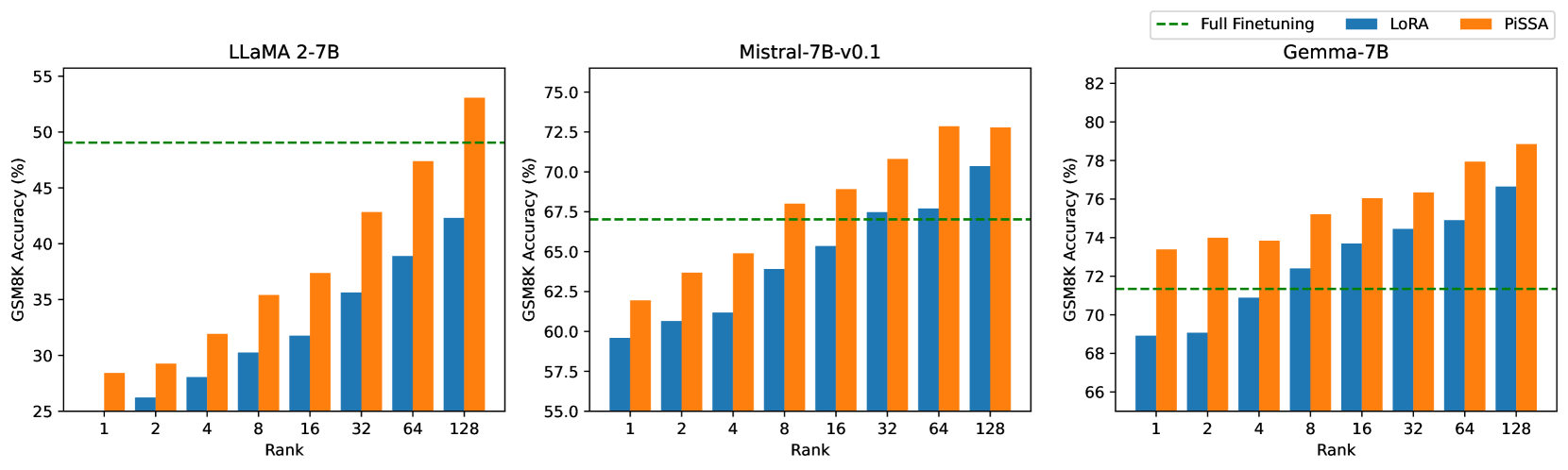
From Figure 14, PiSSA uses fewer trainable parameters compared to LoRA while achieving or even surpassing full-parameter fine-tuning on LLaMA-2-7B and Mistral-7B. Remarkably, on Gemma-7B, PiSSA exceeds full-parameter fine-tuning performance even at rank=1. However, as the rank increases to 128, the performance of PiSSA begins to decline, indicating that PiSSA over-parameterizes earlier than LoRA. This over-parameterization phenomenon does not occur on LLaMA-2-7B, suggesting that increasing the rank further might enable PiSSA to achieve even higher performance on LLaMA-2-7B.

H.3 More Training Loss and Grad Norm under Various Ranks

In Figure 15 and 16, we examining the loss and gradient norm during the training process of PiSSA and LoRA on LLaMA 2-7B, Mistral-7B-v0.1, and Gemma-7B using different ranks.

Figure 15: Comparison of training loss for LLaMA-2-7B, Mistral-7B, and Gemma-7B, organized into three rows, using LoRA and PISSA across ranks $2^i,i\in [0,7]$, organized into eight columns.

Figure 16: Comparison of grad norm for LLaMA-2-7B, Mistral-7B, and Gemma-7B, organized into three rows, using LoRA and PISSA across ranks $2^i,i\in [0,7]$, organized into eight columns.

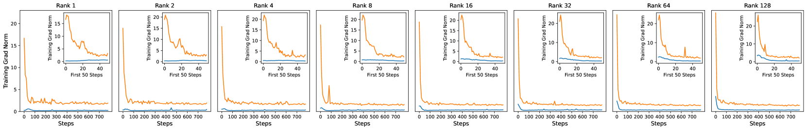
From Figure 15, PiSSA consistently shows a faster initial loss reduction compared to LoRA across various ranks. Additionally, the final loss remains lower than that of LoRA. This advantage is particularly pronounced when the rank is smaller. From Figure 16, the gradient norm of PiSSA remains consistently higher than that of LoRA throughout the training process, indicating its efficient fitting of the training data. A closer look at the first few steps of LoRA’s gradient norm reveals a trend of rising and then falling. According to Section 3, LoRA’s gradients are initially close to zero, leading to very slow model updates. This requires several steps to elevate LoRA’s weights to a higher level before subsequent updates. This phenomenon validates our assertion that LoRA wastes some training steps and therefore converges more slowly. It demonstrates the robustness of the faster convergence property of PiSSA across various ranks.

Appendix I Experimental Settings on NLU

Datasets

We evaluate the performance of PiSSA on GLUE benchmark, including 2 single-sentence classification tasks (CoLA, SST), 5 pairwise text classification tasks (MNLI, RTE, QQP, MRPC and QNLI) and 1 text similarity prediction task (STS-B). We report overall matched and mismatched accuracy on MNLI, Matthew’s correlation on CoLA, Pearson correlation on STS-B, and accuracy on the other datasets.

Implementation Details

To evaluate the performance of PiSSA intuitively, we compared PiSSA and LoRA with the same number of trainable parameters. RoBERTa-large has $355M$ trainable parameters. PiSSA was applied to $W_Q$ and $W_V$, resulting in a total of $1.84M$ trainable parameters. DeBERTa-v3-base has $184M$ trainable parameters. PiSSA and LoRA were applied to $W_Q$, $W_K$ and $W_V$ respectively, resulting in a total of $1.33M$ trainable parameters.

Experiments on NLU are based on the publicly available LoftQ [49] code-base. On RoBERTa-large, we initialize the model with pretrained MNLI checkpoint for the task of MRPC, RTE and STS-B. We set the rank of PiSSA in this experiment as $8$ and selecte lora alpha in 8, 16. We utilize AdamW with linear learning rate schedule to optimize and tune learning rate (LR) from 1e-4,2e-4,3e-4,4e-4,5e-4, 6e-4, 5e-5, 3e-5. Batch sizes (BS) are selected from $6,8,16,32$. Table 7 presents the hyperparmeters we utilized on the glue benchmark.

Table 7: Hyperparameters of our Methods on GLUE.

Dataset	Roberta-large				Deberta-v3-base
	Epoch	BS	LR	Lora alpha	Epoch	BS	LR	Lora alpha
MNLI	10	32	1e-4	16	5	16	5e-5	8
SST-2	10	32	2e-4	16	20	16	3e-5	8
MRPC	20	16	6e-4	8	20	32	2e-4	8
CoLA	20	16	4e-4	8	20	16	1e-4	8
QNLI	10	6	1e-4	8	10	32	1e-4	16
QQP	20	32	3e-4	8	10	16	1e-4	8
RTE	20	16	3e-4	16	50	16	1e-4	8
STS-B	30	16	3e-4	16	20	8	3e-4	8