Intro to Data Structures
我们将首先快速,非全面地概述大熊猫中的基本数据结构,以帮助您入门。 关于数据类型,索引和轴标记/对齐的基本行为适用于所有对象。 首先,将numpy和pandas导入到命名空间中:
In [1]: import numpy as np

In [2]: import pandas as pd
这是一个要记住的基本原则:数据对齐是内在的。 除非您明确说明,否则标签和数据之间的链接不会被破坏。
我们将简要介绍数据结构,然后在单独的部分中考虑所有大类功能和方法。
Series
Series是一维标记数组,能够保存任何数据类型(整数,字符串,浮点数,Python对象等)。 轴标签统称为index。 创建系列的基本方法是调用:
>>> s = pd.Series(data, index=index)
Here, data can be many different things:
- a Python dict
- an ndarray
- a scalar value (like 5)
传递的index是轴标签列表。 Thus, this separates into a few cases depending on what data is:
From ndarray
If data is an ndarray, index must be the same length as data. If no
index is passed, one will be created having values [0, ..., len(data) - 1].
In [3]: s = pd.Series(np.random.randn(5), index=['a', 'b', 'c', 'd', 'e'])

In [4]: s
Out[4]:
a    0.4691
b   -0.2829
c   -1.5091
d   -1.1356
e    1.2121
dtype: float64

In [5]: s.index
Out[5]: Index(['a', 'b', 'c', 'd', 'e'], dtype='object')

In [6]: pd.Series(np.random.randn(5))
Out[6]:
0   -0.1732
1    0.1192
2   -1.0442
3   -0.8618
4   -2.1046
dtype: float64
Note
pandas supports non-unique index values. If an operation that does not support duplicate index values is attempted, an exception will be raised at that time. The reason for being lazy is nearly all performance-based (there are many instances in computations, like parts of GroupBy, where the index is not used).
From dict
如果data是dict,如果传递index,则将拉出与索引中的标签对应的数据中的值。 否则,如果可能,将从dict的排序键构造索引。
In [7]: d = {'a' : 0., 'b' : 1., 'c' : 2.}

In [8]: pd.Series(d)
Out[8]:
a    0.0
b    1.0
c    2.0
dtype: float64

In [9]: pd.Series(d, index=['b', 'c', 'd', 'a'])
Out[9]:
b    1.0
c    2.0
d    NaN
a    0.0
dtype: float64
Note
NaN(not a number)是pandas中使用的标准缺失数据标记
从标量值如果data是标量值,则必须提供索引。 将重复该值以匹配index的长度
In [10]: pd.Series(5., index=['a', 'b', 'c', 'd', 'e'])
Out[10]:
a    5.0
b    5.0
c    5.0
d    5.0
e    5.0
dtype: float64
Series is ndarray-like
Series与ndarray非常相似,是大多数NumPy函数的有效参数。
但是,像切片这样的东西也会对索引进行切片。
In [11]: s[0]
Out[11]: 0.46911229990718628

In [12]: s[:3]
Out[12]:
a    0.4691
b   -0.2829
c   -1.5091
dtype: float64

In [13]: s[s > s.median()]
Out[13]:
a    0.4691
e    1.2121
dtype: float64

In [14]: s[[4, 3, 1]]
Out[14]:
e    1.2121
d   -1.1356
b   -0.2829
dtype: float64

In [15]: np.exp(s)
Out[15]:
a    1.5986
b    0.7536
c    0.2211
d    0.3212
e    3.3606
dtype: float64
我们将在单独的部分中解决基于数组的索引。
Series is dict-like
Series类似于固定大小的dict,您可以通过索引标签获取和设置值:
In [16]: s['a']
Out[16]: 0.46911229990718628

In [17]: s['e'] = 12.

In [18]: s
Out[18]:
a     0.4691
b    -0.2829
c    -1.5091
d    -1.1356
e    12.0000
dtype: float64

In [19]: 'e' in s
Out[19]: True

In [20]: 'f' in s
Out[20]: False
如果未包含标签,则会引发异常:
>>> s['f']
KeyError: 'f'
使用get方法,缺少的标签将返回None或指定的默认值:
In [21]: s.get('f')

In [22]: s.get('f', np.nan)
Out[22]: nan
See also the section on attribute access.
使用Series ¶进行矢量化操作和标签对齐
在进行数据分析时,与通过系列逐个值循环的原始NumPy数组一样,通常不需要。 Sweies也可以传递到大多数期待ndarray的NumPy方法。
In [23]: s + s
Out[23]:
a     0.9382
b    -0.5657
c    -3.0181
d    -2.2713
e    24.0000
dtype: float64

In [24]: s * 2
Out[24]:
a     0.9382
b    -0.5657
c    -3.0181
d    -2.2713
e    24.0000
dtype: float64

In [25]: np.exp(s)
Out[25]:
a         1.5986
b         0.7536
c         0.2211
d         0.3212
e    162754.7914
dtype: float64
Series和ndarray之间的主要区别在于Series之间的操作会根据标签自动对齐数据。 因此,您可以在不考虑所涉及的系列是否具有相同标签的情况下编写计算。
In [26]: s[1:] + s[:-1]
Out[26]:
a       NaN
b   -0.5657
c   -3.0181
d   -2.2713
e       NaN
dtype: float64
未对齐系列之间的操作结果将包含所涉及索引的union。 如果在一个系列或另一个Series中找不到标签,结果将被标记为缺少NaN。 能够在不进行任何明确数据对齐的情况下编写代码,可以在交互式数据分析和研究中获得巨大的自由度和灵活性。 除了用于处理标记数据的大多数相关工具之外,pandas数据结构的集成数据对齐功能设置了pandas。
Note
In general, we chose to make the default result of operations between differently indexed objects yield the union of the indexes in order to avoid loss of information. Having an index label, though the data is missing, is typically important information as part of a computation. You of course have the option of dropping labels with missing data via the dropna function.
Name attribute
系列还可以具有name属性:
In [27]: s = pd.Series(np.random.randn(5), name='something')

In [28]: s
Out[28]:
0   -0.4949
1    1.0718
2    0.7216
3   -0.7068
4   -1.0396
Name: something, dtype: float64

In [29]: s.name
Out[29]: 'something'
在许多情况下,Seriesname将自动分配,特别是在获取1D切片的DataFrame时,如下所示。
New in version 0.18.0.
You can rename a Series with the pandas.Series.rename() method.
In [30]: s2 = s.rename("different")

In [31]: s2.name
Out[31]: 'different'
Note that s and s2 refer to different objects.
DataFrame
DataFrame是具有可能不同类型的列的二维标记数据结构。 您可以将其视为电子表格或SQL表,或Series对象的字典。 它通常是最常用的pandas对象。 与Series类似,DataFrame接受许多不同类型的输入:
- Dict of 1D ndarrays, lists, dicts, or Series
- 2-D numpy.ndarray
- Structured or record ndarray
- A
Series- Another
DataFrame
除数据外,您还可以选择传递index(行标签)和columns(列标签)参数。 如果传递索引和/或列,则可以保证生成的DataFrame的索引和/或列。 因此,系列的字典加上特定索引将丢弃与传递的索引不匹配的所有数据。
如果未传递轴标签,则将根据常识规则从输入数据构造它们。
From dict of Series or dicts
The result index will be the union of the indexes of the various Series. If there are any nested dicts, these will be first converted to Series. If no columns are passed, the columns will be the sorted list of dict keys.
In [32]: d = {'one' : pd.Series([1., 2., 3.], index=['a', 'b', 'c']),
   ....:      'two' : pd.Series([1., 2., 3., 4.], index=['a', 'b', 'c', 'd'])}
   ....:

In [33]: df = pd.DataFrame(d)

In [34]: df
Out[34]:
   one  two
a  1.0  1.0
b  2.0  2.0
c  3.0  3.0
d  NaN  4.0

In [35]: pd.DataFrame(d, index=['d', 'b', 'a'])
Out[35]:
   one  two
d  NaN  4.0
b  2.0  2.0
a  1.0  1.0

In [36]: pd.DataFrame(d, index=['d', 'b', 'a'], columns=['two', 'three'])
Out[36]:
   two three
d  4.0   NaN
b  2.0   NaN
a  1.0   NaN
The row and column labels can be accessed respectively by accessing the index and columns attributes:
Note
When a particular set of columns is passed along with a dict of data, the passed columns override the keys in the dict.
In [37]: df.index
Out[37]: Index(['a', 'b', 'c', 'd'], dtype='object')

In [38]: df.columns
Out[38]: Index(['one', 'two'], dtype='object')
From dict of ndarrays / lists
The ndarrays must all be the same length. If an index is passed, it must
clearly also be the same length as the arrays. If no index is passed, the
result will be range(n), where n is the array length.
In [39]: d = {'one' : [1., 2., 3., 4.],
   ....:      'two' : [4., 3., 2., 1.]}
   ....:

In [40]: pd.DataFrame(d)
Out[40]:
   one  two
0  1.0  4.0
1  2.0  3.0
2  3.0  2.0
3  4.0  1.0

In [41]: pd.DataFrame(d, index=['a', 'b', 'c', 'd'])
Out[41]:
   one  two
a  1.0  4.0
b  2.0  3.0
c  3.0  2.0
d  4.0  1.0
From structured or record array
This case is handled identically to a dict of arrays.
In [42]: data = np.zeros((2,), dtype=[('A', 'i4'),('B', 'f4'),('C', 'a10')])

In [43]: data[:] = [(1,2.,'Hello'), (2,3.,"World")]

In [44]: pd.DataFrame(data)
Out[44]:
   A    B         C
0  1  2.0  b'Hello'
1  2  3.0  b'World'

In [45]: pd.DataFrame(data, index=['first', 'second'])
Out[45]:
        A    B         C
first   1  2.0  b'Hello'
second  2  3.0  b'World'

In [46]: pd.DataFrame(data, columns=['C', 'A', 'B'])
Out[46]:
          C  A    B
0  b'Hello'  1  2.0
1  b'World'  2  3.0
Note
DataFrame is not intended to work exactly like a 2-dimensional NumPy ndarray.
From a list of dicts
In [47]: data2 = [{'a': 1, 'b': 2}, {'a': 5, 'b': 10, 'c': 20}]

In [48]: pd.DataFrame(data2)
Out[48]:
   a   b     c
0  1   2   NaN
1  5  10  20.0

In [49]: pd.DataFrame(data2, index=['first', 'second'])
Out[49]:
        a   b     c
first   1   2   NaN
second  5  10  20.0

In [50]: pd.DataFrame(data2, columns=['a', 'b'])
Out[50]:
   a   b
0  1   2
1  5  10
From a dict of tuples
You can automatically create a multi-indexed frame by passing a tuples dictionary
In [51]: pd.DataFrame({('a', 'b'): {('A', 'B'): 1, ('A', 'C'): 2},
   ....:               ('a', 'a'): {('A', 'C'): 3, ('A', 'B'): 4},
   ....:               ('a', 'c'): {('A', 'B'): 5, ('A', 'C'): 6},
   ....:               ('b', 'a'): {('A', 'C'): 7, ('A', 'B'): 8},
   ....:               ('b', 'b'): {('A', 'D'): 9, ('A', 'B'): 10}})
   ....:
Out[51]:
       a              b
       a    b    c    a     b
A B  4.0  1.0  5.0  8.0  10.0
  C  3.0  2.0  6.0  7.0   NaN
  D  NaN  NaN  NaN  NaN   9.0
From a Series
The result will be a DataFrame with the same index as the input Series, and with one column whose name is the original name of the Series (only if no other column name provided).
Missing Data
Much more will be said on this topic in the Missing data
section. To construct a DataFrame with missing data, use np.nan for those
values which are missing. Alternatively, you may pass a numpy.MaskedArray
as the data argument to the DataFrame constructor, and its masked entries will
be considered missing.
Alternate Constructors
DataFrame.from_dict
DataFrame.from_dict takes a dict of dicts or a dict of array-like sequences
and returns a DataFrame. It operates like the DataFrame constructor except
for the orient parameter which is 'columns' by default, but which can be
set to 'index' in order to use the dict keys as row labels.
DataFrame.from_records
DataFrame.from_records takes a list of tuples or an ndarray with structured
dtype. Works analogously to the normal DataFrame constructor, except that
index maybe be a specific field of the structured dtype to use as the index.
For example:
In [52]: data
Out[52]:
array([(1,  2., b'Hello'), (2,  3., b'World')],
      dtype=[('A', '<i4'), ('B', '<f4'), ('C', 'S10')])

In [53]: pd.DataFrame.from_records(data, index='C')
Out[53]:
          A    B
C
b'Hello'  1  2.0
b'World'  2  3.0
DataFrame.from_items
DataFrame.from_items works analogously to the form of the dict
constructor that takes a sequence of (key, value) pairs, where the keys are
column (or row, in the case of orient='index') names, and the value are the
column values (or row values). This can be useful for constructing a DataFrame
with the columns in a particular order without having to pass an explicit list
of columns:
In [54]: pd.DataFrame.from_items([('A', [1, 2, 3]), ('B', [4, 5, 6])])
Out[54]:
   A  B
0  1  4
1  2  5
2  3  6
If you pass orient='index', the keys will be the row labels. But in this
case you must also pass the desired column names:
In [55]: pd.DataFrame.from_items([('A', [1, 2, 3]), ('B', [4, 5, 6])],
   ....:                         orient='index', columns=['one', 'two', 'three'])
   ....:
Out[55]:
   one  two  three
A    1    2      3
B    4    5      6
Column selection, addition, deletion
You can treat a DataFrame semantically like a dict of like-indexed Series objects. Getting, setting, and deleting columns works with the same syntax as the analogous dict operations:
In [56]: df['one']
Out[56]:
a    1.0
b    2.0
c    3.0
d    NaN
Name: one, dtype: float64

In [57]: df['three'] = df['one'] * df['two']

In [58]: df['flag'] = df['one'] > 2

In [59]: df
Out[59]:
   one  two  three   flag
a  1.0  1.0    1.0  False
b  2.0  2.0    4.0  False
c  3.0  3.0    9.0   True
d  NaN  4.0    NaN  False
Columns can be deleted or popped like with a dict:
In [60]: del df['two']

In [61]: three = df.pop('three')

In [62]: df
Out[62]:
   one   flag
a  1.0  False
b  2.0  False
c  3.0   True
d  NaN  False
When inserting a scalar value, it will naturally be propagated to fill the column:
In [63]: df['foo'] = 'bar'

In [64]: df
Out[64]:
   one   flag  foo
a  1.0  False  bar
b  2.0  False  bar
c  3.0   True  bar
d  NaN  False  bar
When inserting a Series that does not have the same index as the DataFrame, it will be conformed to the DataFrame’s index:
In [65]: df['one_trunc'] = df['one'][:2]

In [66]: df
Out[66]:
   one   flag  foo  one_trunc
a  1.0  False  bar        1.0
b  2.0  False  bar        2.0
c  3.0   True  bar        NaN
d  NaN  False  bar        NaN
You can insert raw ndarrays but their length must match the length of the DataFrame’s index.
By default, columns get inserted at the end. The insert function is
available to insert at a particular location in the columns:
In [67]: df.insert(1, 'bar', df['one'])

In [68]: df
Out[68]:
   one  bar   flag  foo  one_trunc
a  1.0  1.0  False  bar        1.0
b  2.0  2.0  False  bar        2.0
c  3.0  3.0   True  bar        NaN
d  NaN  NaN  False  bar        NaN
Assigning New Columns in Method Chains
Inspired by dplyr’s
mutate verb, DataFrame has an assign()
method that allows you to easily create new columns that are potentially
derived from existing columns.
In [69]: iris = pd.read_csv('data/iris.data')

In [70]: iris.head()
Out[70]:
   SepalLength  SepalWidth  PetalLength  PetalWidth         Name
0          5.1         3.5          1.4         0.2  Iris-setosa
1          4.9         3.0          1.4         0.2  Iris-setosa
2          4.7         3.2          1.3         0.2  Iris-setosa
3          4.6         3.1          1.5         0.2  Iris-setosa
4          5.0         3.6          1.4         0.2  Iris-setosa

In [71]: (iris.assign(sepal_ratio = iris['SepalWidth'] / iris['SepalLength'])
   ....:      .head())
   ....:
Out[71]:
   SepalLength  SepalWidth  PetalLength  PetalWidth         Name  sepal_ratio
0          5.1         3.5          1.4         0.2  Iris-setosa       0.6863
1          4.9         3.0          1.4         0.2  Iris-setosa       0.6122
2          4.7         3.2          1.3         0.2  Iris-setosa       0.6809
3          4.6         3.1          1.5         0.2  Iris-setosa       0.6739
4          5.0         3.6          1.4         0.2  Iris-setosa       0.7200
Above was an example of inserting a precomputed value. We can also pass in a function of one argument to be evalutated on the DataFrame being assigned to.
In [72]: iris.assign(sepal_ratio = lambda x: (x['SepalWidth'] /
   ....:                                      x['SepalLength'])).head()
   ....:
Out[72]:
   SepalLength  SepalWidth  PetalLength  PetalWidth         Name  sepal_ratio
0          5.1         3.5          1.4         0.2  Iris-setosa       0.6863
1          4.9         3.0          1.4         0.2  Iris-setosa       0.6122
2          4.7         3.2          1.3         0.2  Iris-setosa       0.6809
3          4.6         3.1          1.5         0.2  Iris-setosa       0.6739
4          5.0         3.6          1.4         0.2  Iris-setosa       0.7200
assign always returns a copy of the data, leaving the original
DataFrame untouched.
Passing a callable, as opposed to an actual value to be inserted, is
useful when you don’t have a reference to the DataFrame at hand. This is
common when using assign in chains of operations. For example,
we can limit the DataFrame to just those observations with a Sepal Length
greater than 5, calculate the ratio, and plot:
In [73]: (iris.query('SepalLength > 5')
   ....:      .assign(SepalRatio = lambda x: x.SepalWidth / x.SepalLength,
   ....:              PetalRatio = lambda x: x.PetalWidth / x.PetalLength)
   ....:      .plot(kind='scatter', x='SepalRatio', y='PetalRatio'))
   ....:
Out[73]: <matplotlib.axes._subplots.AxesSubplot at 0x1197dd908>
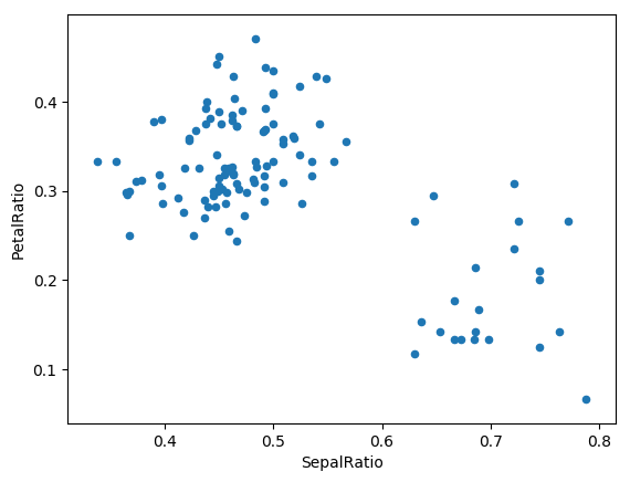
Since a function is passed in, the function is computed on the DataFrame being assigned to. Importantly, this is the DataFrame that’s been filtered to those rows with sepal length greater than 5. The filtering happens first, and then the ratio calculations. This is an example where we didn’t have a reference to the filtered DataFrame available.
The function signature for assign is simply **kwargs. The keys
are the column names for the new fields, and the values are either a value
to be inserted (for example, a Series or NumPy array), or a function
of one argument to be called on the DataFrame. A copy of the original
DataFrame is returned, with the new values inserted.
Warning
Since the function signature of assign is **kwargs, a dictionary,
the order of the new columns in the resulting DataFrame cannot be guaranteed
to match the order you pass in. To make things predictable, items are inserted
alphabetically (by key) at the end of the DataFrame.
All expressions are computed first, and then assigned. So you can’t refer
to another column being assigned in the same call to assign. For example:
In [74]: # Don't do this, bad reference to `C`
        df.assign(C = lambda x: x['A'] + x['B'],
                  D = lambda x: x['A'] + x['C'])
In [2]: # Instead, break it into two assigns
        (df.assign(C = lambda x: x['A'] + x['B'])
           .assign(D = lambda x: x['A'] + x['C']))
Indexing / Selection
The basics of indexing are as follows:
| Operation | Syntax | Result |
|---|---|---|
| Select column | df[col] |
Series |
| Select row by label | df.loc[label] |
Series |
| Select row by integer location | df.iloc[loc] |
Series |
| Slice rows | df[5:10] |
DataFrame |
| Select rows by boolean vector | df[bool_vec] |
DataFrame |
Row selection, for example, returns a Series whose index is the columns of the DataFrame:
In [75]: df.loc['b']
Out[75]:
one              2
bar              2
flag         False
foo            bar
one_trunc        2
Name: b, dtype: object

In [76]: df.iloc[2]
Out[76]:
one             3
bar             3
flag         True
foo           bar
one_trunc     NaN
Name: c, dtype: object
For a more exhaustive treatment of more sophisticated label-based indexing and slicing, see the section on indexing. We will address the fundamentals of reindexing / conforming to new sets of labels in the section on reindexing.
Data alignment and arithmetic
Data alignment between DataFrame objects automatically align on both the columns and the index (row labels). Again, the resulting object will have the union of the column and row labels.
In [77]: df = pd.DataFrame(np.random.randn(10, 4), columns=['A', 'B', 'C', 'D'])

In [78]: df2 = pd.DataFrame(np.random.randn(7, 3), columns=['A', 'B', 'C'])

In [79]: df + df2
Out[79]:
        A       B       C   D
0  0.0457 -0.0141  1.3809 NaN
1 -0.9554 -1.5010  0.0372 NaN
2 -0.6627  1.5348 -0.8597 NaN
3 -2.4529  1.2373 -0.1337 NaN
4  1.4145  1.9517 -2.3204 NaN
5 -0.4949 -1.6497 -1.0846 NaN
6 -1.0476 -0.7486 -0.8055 NaN
7     NaN     NaN     NaN NaN
8     NaN     NaN     NaN NaN
9     NaN     NaN     NaN NaN
When doing an operation between DataFrame and Series, the default behavior is to align the Series index on the DataFrame columns, thus broadcasting row-wise. For example:
In [80]: df - df.iloc[0]
Out[80]:
        A       B       C       D
0  0.0000  0.0000  0.0000  0.0000
1 -1.3593 -0.2487 -0.4534 -1.7547
2  0.2531  0.8297  0.0100 -1.9912
3 -1.3111  0.0543 -1.7249 -1.6205
4  0.5730  1.5007 -0.6761  1.3673
5 -1.7412  0.7820 -1.2416 -2.0531
6 -1.2408 -0.8696 -0.1533  0.0004
7 -0.7439  0.4110 -0.9296 -0.2824
8 -1.1949  1.3207  0.2382 -1.4826
9  2.2938  1.8562  0.7733 -1.4465
In the special case of working with time series data, and the DataFrame index also contains dates, the broadcasting will be column-wise:
In [81]: index = pd.date_range('1/1/2000', periods=8)

In [82]: df = pd.DataFrame(np.random.randn(8, 3), index=index, columns=list('ABC'))

In [83]: df
Out[83]:
                 A       B       C
2000-01-01 -1.2268  0.7698 -1.2812
2000-01-02 -0.7277 -0.1213 -0.0979
2000-01-03  0.6958  0.3417  0.9597
2000-01-04 -1.1103 -0.6200  0.1497
2000-01-05 -0.7323  0.6877  0.1764
2000-01-06  0.4033 -0.1550  0.3016
2000-01-07 -2.1799 -1.3698 -0.9542
2000-01-08  1.4627 -1.7432 -0.8266

In [84]: type(df['A'])
Out[84]: pandas.core.series.Series

In [85]: df - df['A']
Out[85]:
            2000-01-01 00:00:00  2000-01-02 00:00:00  2000-01-03 00:00:00  \
2000-01-01                  NaN                  NaN                  NaN
2000-01-02                  NaN                  NaN                  NaN
2000-01-03                  NaN                  NaN                  NaN
2000-01-04                  NaN                  NaN                  NaN
2000-01-05                  NaN                  NaN                  NaN
2000-01-06                  NaN                  NaN                  NaN
2000-01-07                  NaN                  NaN                  NaN
2000-01-08                  NaN                  NaN                  NaN

            2000-01-04 00:00:00 ...  2000-01-08 00:00:00   A   B   C
2000-01-01                  NaN ...                  NaN NaN NaN NaN
2000-01-02                  NaN ...                  NaN NaN NaN NaN
2000-01-03                  NaN ...                  NaN NaN NaN NaN
2000-01-04                  NaN ...                  NaN NaN NaN NaN
2000-01-05                  NaN ...                  NaN NaN NaN NaN
2000-01-06                  NaN ...                  NaN NaN NaN NaN
2000-01-07                  NaN ...                  NaN NaN NaN NaN
2000-01-08                  NaN ...                  NaN NaN NaN NaN

[8 rows x 11 columns]
Warning
df - df['A']
is now deprecated and will be removed in a future release. The preferred way to replicate this behavior is
df.sub(df['A'], axis=0)
For explicit control over the matching and broadcasting behavior, see the section on flexible binary operations.
Operations with scalars are just as you would expect:
In [86]: df * 5 + 2
Out[86]:
                 A       B       C
2000-01-01 -4.1341  5.8490 -4.4062
2000-01-02 -1.6385  1.3935  1.5106
2000-01-03  5.4789  3.7087  6.7986
2000-01-04 -3.5517 -1.0999  2.7487
2000-01-05 -1.6617  5.4387  2.8822
2000-01-06  4.0165  1.2252  3.5081
2000-01-07 -8.8993 -4.8492 -2.7710
2000-01-08  9.3135 -6.7158 -2.1330

In [87]: 1 / df
Out[87]:
                 A       B        C
2000-01-01 -0.8151  1.2990  -0.7805
2000-01-02 -1.3742 -8.2436 -10.2163
2000-01-03  1.4372  2.9262   1.0420
2000-01-04 -0.9006 -1.6130   6.6779
2000-01-05 -1.3655  1.4540   5.6675
2000-01-06  2.4795 -6.4537   3.3154
2000-01-07 -0.4587 -0.7300  -1.0480
2000-01-08  0.6837 -0.5737  -1.2098

In [88]: df ** 4
Out[88]:
                  A       B           C
2000-01-01   2.2653  0.3512  2.6948e+00
2000-01-02   0.2804  0.0002  9.1796e-05
2000-01-03   0.2344  0.0136  8.4838e-01
2000-01-04   1.5199  0.1477  5.0286e-04
2000-01-05   0.2876  0.2237  9.6924e-04
2000-01-06   0.0265  0.0006  8.2769e-03
2000-01-07  22.5795  3.5212  8.2903e-01
2000-01-08   4.5774  9.2332  4.6683e-01
Boolean operators work as well:
In [89]: df1 = pd.DataFrame({'a' : [1, 0, 1], 'b' : [0, 1, 1] }, dtype=bool)

In [90]: df2 = pd.DataFrame({'a' : [0, 1, 1], 'b' : [1, 1, 0] }, dtype=bool)

In [91]: df1 & df2
Out[91]:
       a      b
0  False  False
1  False   True
2   True  False

In [92]: df1 | df2
Out[92]:
      a     b
0  True  True
1  True  True
2  True  True

In [93]: df1 ^ df2
Out[93]:
       a      b
0   True   True
1   True  False
2  False   True

In [94]: -df1
Out[94]:
       a      b
0  False   True
1   True  False
2  False  False
Transposing
To transpose, access the T attribute (also the transpose function),
similar to an ndarray:
# only show the first 5 rows
In [95]: df[:5].T
Out[95]:
   2000-01-01  2000-01-02  2000-01-03  2000-01-04  2000-01-05
A     -1.2268     -0.7277      0.6958     -1.1103     -0.7323
B      0.7698     -0.1213      0.3417     -0.6200      0.6877
C     -1.2812     -0.0979      0.9597      0.1497      0.1764
DataFrame interoperability with NumPy functions
Elementwise NumPy ufuncs (log, exp, sqrt, ...) and various other NumPy functions can be used with no issues on DataFrame, assuming the data within are numeric:
In [96]: np.exp(df)
Out[96]:
                 A       B       C
2000-01-01  0.2932  2.1593  0.2777
2000-01-02  0.4830  0.8858  0.9068
2000-01-03  2.0053  1.4074  2.6110
2000-01-04  0.3294  0.5380  1.1615
2000-01-05  0.4808  1.9892  1.1930
2000-01-06  1.4968  0.8565  1.3521
2000-01-07  0.1131  0.2541  0.3851
2000-01-08  4.3176  0.1750  0.4375

In [97]: np.asarray(df)
Out[97]:
array([[-1.2268,  0.7698, -1.2812],
       [-0.7277, -0.1213, -0.0979],
       [ 0.6958,  0.3417,  0.9597],
       [-1.1103, -0.62  ,  0.1497],
       [-0.7323,  0.6877,  0.1764],
       [ 0.4033, -0.155 ,  0.3016],
       [-2.1799, -1.3698, -0.9542],
       [ 1.4627, -1.7432, -0.8266]])
The dot method on DataFrame implements matrix multiplication:
In [98]: df.T.dot(df)
Out[98]:
         A       B       C
A  11.3419 -0.0598  3.0080
B  -0.0598  6.5206  2.0833
C   3.0080  2.0833  4.3105
Similarly, the dot method on Series implements dot product:
In [99]: s1 = pd.Series(np.arange(5,10))

In [100]: s1.dot(s1)
Out[100]: 255
DataFrame is not intended to be a drop-in replacement for ndarray as its indexing semantics are quite different in places from a matrix.
Console display
Very large DataFrames will be truncated to display them in the console.
You can also get a summary using info().
(Here I am reading a CSV version of the baseball dataset from the plyr
R package):
In [101]: baseball = pd.read_csv('data/baseball.csv')

In [102]: print(baseball)
       id     player  year  stint  ...   hbp   sh   sf  gidp
0   88641  womacto01  2006      2  ...   0.0  3.0  0.0   0.0
1   88643  schilcu01  2006      1  ...   0.0  0.0  0.0   0.0
..    ...        ...   ...    ...  ...   ...  ...  ...   ...
98  89533   aloumo01  2007      1  ...   2.0  0.0  3.0  13.0
99  89534  alomasa02  2007      1  ...   0.0  0.0  0.0   0.0

[100 rows x 23 columns]

In [103]: baseball.info()
<class 'pandas.core.frame.DataFrame'>
RangeIndex: 100 entries, 0 to 99
Data columns (total 23 columns):
id        100 non-null int64
player    100 non-null object
year      100 non-null int64
stint     100 non-null int64
team      100 non-null object
lg        100 non-null object
g         100 non-null int64
ab        100 non-null int64
r         100 non-null int64
h         100 non-null int64
X2b       100 non-null int64
X3b       100 non-null int64
hr        100 non-null int64
rbi       100 non-null float64
sb        100 non-null float64
cs        100 non-null float64
bb        100 non-null int64
so        100 non-null float64
ibb       100 non-null float64
hbp       100 non-null float64
sh        100 non-null float64
sf        100 non-null float64
gidp      100 non-null float64
dtypes: float64(9), int64(11), object(3)
memory usage: 18.0+ KB
However, using to_string will return a string representation of the
DataFrame in tabular form, though it won’t always fit the console width:
In [104]: print(baseball.iloc[-20:, :12].to_string())
       id     player  year  stint team  lg    g   ab   r    h  X2b  X3b
80  89474  finlest01  2007      1  COL  NL   43   94   9   17    3    0
81  89480  embreal01  2007      1  OAK  AL    4    0   0    0    0    0
82  89481  edmonji01  2007      1  SLN  NL  117  365  39   92   15    2
83  89482  easleda01  2007      1  NYN  NL   76  193  24   54    6    0
84  89489  delgaca01  2007      1  NYN  NL  139  538  71  139   30    0
85  89493  cormirh01  2007      1  CIN  NL    6    0   0    0    0    0
86  89494  coninje01  2007      2  NYN  NL   21   41   2    8    2    0
87  89495  coninje01  2007      1  CIN  NL   80  215  23   57   11    1
88  89497  clemero02  2007      1  NYA  AL    2    2   0    1    0    0
89  89498  claytro01  2007      2  BOS  AL    8    6   1    0    0    0
90  89499  claytro01  2007      1  TOR  AL   69  189  23   48   14    0
91  89501  cirilje01  2007      2  ARI  NL   28   40   6    8    4    0
92  89502  cirilje01  2007      1  MIN  AL   50  153  18   40    9    2
93  89521  bondsba01  2007      1  SFN  NL  126  340  75   94   14    0
94  89523  biggicr01  2007      1  HOU  NL  141  517  68  130   31    3
95  89525  benitar01  2007      2  FLO  NL   34    0   0    0    0    0
96  89526  benitar01  2007      1  SFN  NL   19    0   0    0    0    0
97  89530  ausmubr01  2007      1  HOU  NL  117  349  38   82   16    3
98  89533   aloumo01  2007      1  NYN  NL   87  328  51  112   19    1
99  89534  alomasa02  2007      1  NYN  NL    8   22   1    3    1    0
Wide DataFrames will be printed across multiple rows by default:
In [105]: pd.DataFrame(np.random.randn(3, 12))
Out[105]:
         0         1         2         3         4         5         6   \
0 -0.345352  1.314232  0.690579  0.995761  2.396780  0.014871  3.357427
1 -2.182937  0.380396  0.084844  0.432390  1.519970 -0.493662  0.600178
2  0.206053 -0.251905 -2.213588  1.063327  1.266143  0.299368 -0.863838

         7         8         9         10        11
0 -0.317441 -1.236269  0.896171 -0.487602 -0.082240
1  0.274230  0.132885 -0.023688  2.410179  1.450520
2  0.408204 -1.048089 -0.025747 -0.988387  0.094055
You can change how much to print on a single row by setting the display.width
option:
In [106]: pd.set_option('display.width', 40) # default is 80

In [107]: pd.DataFrame(np.random.randn(3, 12))
Out[107]:
         0         1         2   \
0  1.262731  1.289997  0.082423
1  1.126203 -0.977349  1.474071
2  0.758527  1.729689 -0.964980

         3         4         5   \
0 -0.055758  0.536580 -0.489682
1 -0.064034 -1.282782  0.781836
2 -0.845696 -1.340896  1.846883

         6         7         8   \
0  0.369374 -0.034571 -2.484478
1 -1.071357  0.441153  2.353925
2 -1.328865  1.682706 -1.717693

         9         10        11
0 -0.281461  0.030711  0.109121
1  0.583787  0.221471 -0.744471
2  0.888782  0.228440  0.901805
You can adjust the max width of the individual columns by setting display.max_colwidth
In [108]: datafile={'filename': ['filename_01','filename_02'],
   .....:           'path': ["media/user_name/storage/folder_01/filename_01",
   .....:                    "media/user_name/storage/folder_02/filename_02"]}
   .....:

In [109]: pd.set_option('display.max_colwidth',30)

In [110]: pd.DataFrame(datafile)
Out[110]:
      filename  \
0  filename_01
1  filename_02

                            path
0  media/user_name/storage/fo...
1  media/user_name/storage/fo...

In [111]: pd.set_option('display.max_colwidth',100)

In [112]: pd.DataFrame(datafile)
Out[112]:
      filename  \
0  filename_01
1  filename_02

                                            path
0  media/user_name/storage/folder_01/filename_01
1  media/user_name/storage/folder_02/filename_02
You can also disable this feature via the expand_frame_repr option.
This will print the table in one block.
DataFrame column attribute access and IPython completion
If a DataFrame column label is a valid Python variable name, the column can be accessed like attributes:
In [113]: df = pd.DataFrame({'foo1' : np.random.randn(5),
   .....:                    'foo2' : np.random.randn(5)})
   .....:

In [114]: df
Out[114]:
       foo1      foo2
0  1.171216 -0.858447
1  0.520260  0.306996
2 -1.197071 -0.028665
3 -1.066969  0.384316
4 -0.303421  1.574159

In [115]: df.foo1
Out[115]:
0    1.171216
1    0.520260
2   -1.197071
3   -1.066969
4   -0.303421
Name: foo1, dtype: float64
The columns are also connected to the IPython completion mechanism so they can be tab-completed:
In [5]: df.fo<TAB>
df.foo1  df.foo2
Panel
Warning
In 0.20.0, Panel is deprecated and will be removed in
a future version. See the section Deprecate Panel.
Panel is a somewhat less-used, but still important container for 3-dimensional data. The term panel data is derived from econometrics and is partially responsible for the name pandas: pan(el)-da(ta)-s. The names for the 3 axes are intended to give some semantic meaning to describing operations involving panel data and, in particular, econometric analysis of panel data. However, for the strict purposes of slicing and dicing a collection of DataFrame objects, you may find the axis names slightly arbitrary:
- items: axis 0, each item corresponds to a DataFrame contained inside
- major_axis: axis 1, it is the index (rows) of each of the DataFrames
- minor_axis: axis 2, it is the columns of each of the DataFrames
Construction of Panels works about like you would expect:
From 3D ndarray with optional axis labels
In [116]: wp = pd.Panel(np.random.randn(2, 5, 4), items=['Item1', 'Item2'],
   .....:               major_axis=pd.date_range('1/1/2000', periods=5),
   .....:               minor_axis=['A', 'B', 'C', 'D'])
   .....:

In [117]: wp
Out[117]:
<class 'pandas.core.panel.Panel'>
Dimensions: 2 (items) x 5 (major_axis) x 4 (minor_axis)
Items axis: Item1 to Item2
Major_axis axis: 2000-01-01 00:00:00 to 2000-01-05 00:00:00
Minor_axis axis: A to D
From dict of DataFrame objects
In [118]: data = {'Item1' : pd.DataFrame(np.random.randn(4, 3)),
   .....:         'Item2' : pd.DataFrame(np.random.randn(4, 2))}
   .....:

In [119]: pd.Panel(data)
Out[119]:
<class 'pandas.core.panel.Panel'>
Dimensions: 2 (items) x 4 (major_axis) x 3 (minor_axis)
Items axis: Item1 to Item2
Major_axis axis: 0 to 3
Minor_axis axis: 0 to 2
Note that the values in the dict need only be convertible to DataFrame. Thus, they can be any of the other valid inputs to DataFrame as per above.
One helpful factory method is Panel.from_dict, which takes a
dictionary of DataFrames as above, and the following named parameters:
| Parameter | Default | Description |
|---|---|---|
| intersect | False |
drops elements whose indices do not align |
| orient | items |
use minor to use DataFrames’ columns as panel items |
For example, compare to the construction above:
In [120]: pd.Panel.from_dict(data, orient='minor')
Out[120]:
<class 'pandas.core.panel.Panel'>
Dimensions: 3 (items) x 4 (major_axis) x 2 (minor_axis)
Items axis: 0 to 2
Major_axis axis: 0 to 3
Minor_axis axis: Item1 to Item2
Orient is especially useful for mixed-type DataFrames. If you pass a dict of
DataFrame objects with mixed-type columns, all of the data will get upcasted to
dtype=object unless you pass orient='minor':
In [121]: df = pd.DataFrame({'a': ['foo', 'bar', 'baz'],
   .....:                    'b': np.random.randn(3)})
   .....:

In [122]: df
Out[122]:
     a         b
0  foo -0.308853
1  bar -0.681087
2  baz  0.377953

In [123]: data = {'item1': df, 'item2': df}

In [124]: panel = pd.Panel.from_dict(data, orient='minor')

In [125]: panel['a']
Out[125]:
  item1 item2
0   foo   foo
1   bar   bar
2   baz   baz

In [126]: panel['b']
Out[126]:
      item1     item2
0 -0.308853 -0.308853
1 -0.681087 -0.681087
2  0.377953  0.377953

In [127]: panel['b'].dtypes
Out[127]:
item1    float64
item2    float64
dtype: object
Note
Panel, being less commonly used than Series and DataFrame, has been slightly neglected feature-wise. A number of methods and options available in DataFrame are not available in Panel.
From DataFrame using to_panel method
to_panel converts a DataFrame with a two-level index to a Panel.
In [128]: midx = pd.MultiIndex(levels=[['one', 'two'], ['x','y']], labels=[[1,1,0,0],[1,0,1,0]])

In [129]: df = pd.DataFrame({'A' : [1, 2, 3, 4], 'B': [5, 6, 7, 8]}, index=midx)

In [130]: df.to_panel()
Out[130]:
<class 'pandas.core.panel.Panel'>
Dimensions: 2 (items) x 2 (major_axis) x 2 (minor_axis)
Items axis: A to B
Major_axis axis: one to two
Minor_axis axis: x to y
Item selection / addition / deletion
Similar to DataFrame functioning as a dict of Series, Panel is like a dict of DataFrames:
In [131]: wp['Item1']
Out[131]:
                   A         B         C         D
2000-01-01  1.588931  0.476720  0.473424 -0.242861
2000-01-02 -0.014805 -0.284319  0.650776 -1.461665
2000-01-03 -1.137707 -0.891060 -0.693921  1.613616
2000-01-04  0.464000  0.227371 -0.496922  0.306389
2000-01-05 -2.290613 -1.134623 -1.561819 -0.260838

In [132]: wp['Item3'] = wp['Item1'] / wp['Item2']
The API for insertion and deletion is the same as for DataFrame. And as with DataFrame, if the item is a valid python identifier, you can access it as an attribute and tab-complete it in IPython.
Transposing
A Panel can be rearranged using its transpose method (which does not make a
copy by default unless the data are heterogeneous):
In [133]: wp.transpose(2, 0, 1)
Out[133]:
<class 'pandas.core.panel.Panel'>
Dimensions: 4 (items) x 3 (major_axis) x 5 (minor_axis)
Items axis: A to D
Major_axis axis: Item1 to Item3
Minor_axis axis: 2000-01-01 00:00:00 to 2000-01-05 00:00:00
Indexing / Selection
| Operation | Syntax | Result |
|---|---|---|
| Select item | wp[item] |
DataFrame |
| Get slice at major_axis label | wp.major_xs(val) |
DataFrame |
| Get slice at minor_axis label | wp.minor_xs(val) |
DataFrame |
For example, using the earlier example data, we could do:
In [134]: wp['Item1']
Out[134]:
                   A         B         C         D
2000-01-01  1.588931  0.476720  0.473424 -0.242861
2000-01-02 -0.014805 -0.284319  0.650776 -1.461665
2000-01-03 -1.137707 -0.891060 -0.693921  1.613616
2000-01-04  0.464000  0.227371 -0.496922  0.306389
2000-01-05 -2.290613 -1.134623 -1.561819 -0.260838

In [135]: wp.major_xs(wp.major_axis[2])
Out[135]:
      Item1     Item2     Item3
A -1.137707  0.800193 -1.421791
B -0.891060  0.782098 -1.139320
C -0.693921 -1.069094  0.649074
D  1.613616 -1.099248 -1.467927

In [136]: wp.minor_axis
Out[136]: Index(['A', 'B', 'C', 'D'], dtype='object')

In [137]: wp.minor_xs('C')
Out[137]:
               Item1     Item2     Item3
2000-01-01  0.473424 -0.902937 -0.524316
2000-01-02  0.650776 -1.144073 -0.568824
2000-01-03 -0.693921 -1.069094  0.649074
2000-01-04 -0.496922  0.661084 -0.751678
2000-01-05 -1.561819 -1.056652  1.478083
Squeezing
Another way to change the dimensionality of an object is to squeeze a 1-len object, similar to wp['Item1']
In [138]: wp.reindex(items=['Item1']).squeeze()
Out[138]:
                   A         B         C         D
2000-01-01  1.588931  0.476720  0.473424 -0.242861
2000-01-02 -0.014805 -0.284319  0.650776 -1.461665
2000-01-03 -1.137707 -0.891060 -0.693921  1.613616
2000-01-04  0.464000  0.227371 -0.496922  0.306389
2000-01-05 -2.290613 -1.134623 -1.561819 -0.260838

In [139]: wp.reindex(items=['Item1'], minor=['B']).squeeze()
Out[139]:
2000-01-01    0.476720
2000-01-02   -0.284319
2000-01-03   -0.891060
2000-01-04    0.227371
2000-01-05   -1.134623
Freq: D, Name: B, dtype: float64
Conversion to DataFrame
A Panel can be represented in 2D form as a hierarchically indexed
DataFrame. See the section hierarchical indexing
for more on this. To convert a Panel to a DataFrame, use the to_frame
method:
In [140]: panel = pd.Panel(np.random.randn(3, 5, 4), items=['one', 'two', 'three'],
   .....:                  major_axis=pd.date_range('1/1/2000', periods=5),
   .....:                  minor_axis=['a', 'b', 'c', 'd'])
   .....:

In [141]: panel.to_frame()
Out[141]:
                       one       two     three
major      minor
2000-01-01 a      0.493672  1.219492 -1.290493
           b     -2.461467  0.062297  0.787872
           c     -1.553902 -0.110388  1.515707
           d      2.015523 -1.184357 -0.276487
2000-01-02 a     -1.833722 -0.558081 -0.223762
           b      1.771740  0.077849  1.397431
           c     -0.670027  0.629498  1.503874
           d      0.049307 -1.035260 -0.478905
2000-01-03 a     -0.521493 -0.438229 -0.135950
           b     -3.201750  0.503703 -0.730327
           c      0.792716  0.413086 -0.033277
           d      0.146111 -1.139050  0.281151
2000-01-04 a      1.903247  0.660342 -1.298915
           b     -0.747169  0.464794 -2.819487
           c     -0.309038 -0.309337 -0.851985
           d      0.393876 -0.649593 -1.106952
2000-01-05 a      1.861468  0.683758 -0.937731
           b      0.936527 -0.643834 -1.537770
           c      1.255746  0.421287  0.555759
           d     -2.655452  1.032814 -2.277282
Deprecate Panel
Over the last few years, pandas has increased in both breadth and depth, with new features,
datatype support, and manipulation routines. As a result, supporting efficient indexing and functional
routines for Series, DataFrame and Panel has contributed to an increasingly fragmented and
difficult-to-understand codebase.
The 3-D structure of a Panel is much less common for many types of data analysis,
than the 1-D of the Series or the 2-D of the DataFrame. Going forward it makes sense for
pandas to focus on these areas exclusively.
Oftentimes, one can simply use a MultiIndex DataFrame for easily working with higher dimensional data.
In additon, the xarray package was built from the ground up, specifically in order to
support the multi-dimensional analysis that is one of Panel s main usecases.
Here is a link to the xarray panel-transition documentation.
In [142]: p = tm.makePanel()

In [143]: p
Out[143]:
<class 'pandas.core.panel.Panel'>
Dimensions: 3 (items) x 30 (major_axis) x 4 (minor_axis)
Items axis: ItemA to ItemC
Major_axis axis: 2000-01-03 00:00:00 to 2000-02-11 00:00:00
Minor_axis axis: A to D
Convert to a MultiIndex DataFrame
In [144]: p.to_frame()
Out[144]:
                     ItemA     ItemB     ItemC
major      minor
2000-01-03 A     -0.390201 -1.624062 -0.605044
           B      1.562443  0.483103  0.583129
           C     -1.085663  0.768159 -0.273458
           D      0.136235 -0.021763 -0.700648
2000-01-04 A      1.207122 -0.758514  0.878404
           B      0.763264  0.061495 -0.876690
           C     -1.114738  0.225441 -0.335117
           D      0.886313 -0.047152 -1.166607
2000-01-05 A      0.178690 -0.560859 -0.921485
           B      0.162027  0.240767 -1.919354
           C     -0.058216  0.543294 -0.476268
           D     -1.350722  0.088472 -0.367236
2000-01-06 A     -1.004168 -0.589005 -0.200312
           B     -0.902704  0.782413 -0.572707
           C     -0.486768  0.771931 -1.765602
           D     -0.886348 -0.857435  1.296674
2000-01-07 A     -1.377627 -1.070678  0.522423
           B      1.106010  0.628462 -1.736484
           C      1.685148 -0.968145  0.578223
           D     -1.013316 -2.503786  0.641385
2000-01-10 A      0.499281 -1.681101  0.722511
           B     -0.199234 -0.880627 -1.335113
           C      0.112572 -1.176383  0.242697
           D      1.920906 -1.058041 -0.779432
2000-01-11 A     -1.405256  0.403776 -1.702486
           B      0.458265  0.777575 -1.244471
           C     -1.495309 -3.192716  0.208129
           D     -0.388231 -0.657981  0.602456
2000-01-12 A      0.162565  0.609862 -0.709535
           B      0.491048 -0.779367  0.347339
...                    ...       ...       ...
2000-02-02 C     -0.303961 -0.463752 -0.288962
           D      0.104050  1.116086  0.506445
2000-02-03 A     -2.338595 -0.581967 -0.801820
           B     -0.557697 -0.033731 -0.176382
           C      0.625555 -0.055289  0.875359
           D      0.174068 -0.443915  1.626369
2000-02-04 A     -0.374279 -1.233862 -0.915751
           B      0.381353 -1.108761 -1.970108
           C     -0.059268 -0.360853 -0.614618
           D     -0.439461 -0.200491  0.429518
2000-02-07 A     -2.359958 -3.520876 -0.288156
           B      1.337122 -0.314399 -1.044208
           C      0.249698  0.728197  0.565375
           D     -0.741343  1.092633  0.013910
2000-02-08 A     -1.157886  0.516870 -1.199945
           B     -1.531095 -0.860626 -0.821179
           C      1.103949  1.326768  0.068184
           D     -0.079673 -1.675194 -0.458272
2000-02-09 A     -0.551865  0.343125 -0.072869
           B      1.331458  0.370397 -1.914267
           C     -1.087532  0.208927  0.788871
           D     -0.922875  0.437234 -1.531004
2000-02-10 A      1.592673  2.137827 -1.828740
           B     -0.571329 -1.761442 -0.826439
           C      1.998044  0.292058 -0.280343
           D      0.303638  0.388254 -0.500569
2000-02-11 A      1.559318  0.452429 -1.716981
           B     -0.026671 -0.899454  0.124808
           C     -0.244548 -2.019610  0.931536
           D     -0.917368  0.479630  0.870690

[120 rows x 3 columns]
Alternatively, one can convert to an xarray DataArray.
In [145]: p.to_xarray()
Out[145]:
<xarray.DataArray (items: 3, major_axis: 30, minor_axis: 4)>
array([[[-0.390201,  1.562443, -1.085663,  0.136235],
        [ 1.207122,  0.763264, -1.114738,  0.886313],
        ...,
        [ 1.592673, -0.571329,  1.998044,  0.303638],
        [ 1.559318, -0.026671, -0.244548, -0.917368]],

       [[-1.624062,  0.483103,  0.768159, -0.021763],
        [-0.758514,  0.061495,  0.225441, -0.047152],
        ...,
        [ 2.137827, -1.761442,  0.292058,  0.388254],
        [ 0.452429, -0.899454, -2.01961 ,  0.47963 ]],

       [[-0.605044,  0.583129, -0.273458, -0.700648],
        [ 0.878404, -0.87669 , -0.335117, -1.166607],
        ...,
        [-1.82874 , -0.826439, -0.280343, -0.500569],
        [-1.716981,  0.124808,  0.931536,  0.87069 ]]])
Coordinates:
  * items       (items) object 'ItemA' 'ItemB' 'ItemC'
  * major_axis  (major_axis) datetime64[ns] 2000-01-03 2000-01-04 2000-01-05 ...
  * minor_axis  (minor_axis) object 'A' 'B' 'C' 'D'
You can see the full-documentation for the xarray package.
Panel4D and PanelND (Deprecated)
Warning
In 0.19.0 Panel4D and PanelND are deprecated and will be removed in
a future version. The recommended way to represent these types of
n-dimensional data are with the
xarray package.
Pandas provides a to_xarray() method to automate
this conversion.
See the docs of a previous version for documentation on these objects.